the Creative Commons Attribution 4.0 License.
the Creative Commons Attribution 4.0 License.
 | 13 Jul 2023
Polar firn properties in Greenland and Antarctica and related effects on microwave brightness temperatures
Haokui Xu
Brooke Medley
Leung Tsang
Joel T. Johnson
Kenneth C. Jezek
Marco Brogioni
Lars Kaleschke
In studying the mass balance of polar ice sheets, fluctuations in firn density near the surface is a major uncertainty. In this paper, we explore these variations at locations on the Greenland Ice Sheet and at the Dome C location in Antarctica. Borehole in situ measurements, snow radar echoes, microwave brightness temperatures, and modeling results from the Community Firn Model (CFM) are used. It is shown that firn density profiles can be represented using three processes: “long-scale” and “short-scale” density variations and “refrozen layers”. Consistency with this description is observed in the dynamic range of airborne 0.5–2 GHz brightness temperatures and snow radar echo peaks in measurements performed in Greenland in 2017. Based on these insights, a new analytical partially coherent model is implemented to explain the microwave brightness temperatures using the three-scale description of the firn. Short- and long-scale firn processes are modeled as a 3D continuous random medium with finite vertical and horizontal correlation lengths as opposed to past 1D randomly layered medium descriptions. Refrozen layers are described as deterministic sheets with planar interfaces, with the number of refrozen-layer interfaces determined by radar observations. Firn density and correlation length parameters used in forward modeling to match measured 0.5–2 GHz brightness temperatures in Greenland show consistency with similar parameters in CFM predictions. Model predictions also are in good agreement with multi-angle 1.4 GHz vertically and horizontally polarized brightness temperature measured by the Soil Moisture and Ocean Salinity (SMOS) satellite at Dome C, Antarctica. This work shows that co-located active and passive microwave measurements can be used to infer polar firn properties that can be compared with predictions of the CFM. In particular, 0.5–2 GHz brightness temperature measurements are shown to be sensitive to long-scale firn density fluctuations with density standard deviations in the range of 0.01–0.06 g cm−3 and vertical correlation lengths of 6–20 cm.
- Article
(1235 KB) - Full-text XML
- BibTeX
- EndNote


The mass balance of polar ice sheets is a major topic in the study of climate change. The most recent assessment of the mass balance of the Greenland and Antarctic ice sheets confirmed a loss of ice to the ocean at a rate of 320 Gt yr−1, equivalent to 1 mm yr−1 sea level rise since 2003 (Smith et al., 2020). The quantification of uncertainty in ice sheet volume change between NASA's first- and second-generation Ice, Cloud, and land Elevation Satellite (ICESat, ICESat-2) missions is a testament to the precision of these laser altimeters. For example, uncertainties for the grounded Antarctica Ice Sheet (AIS) and Greenland Ice Sheet (GrIS) are currently ∼ 5 and 3 km3 yr−1, respectively, as compared to volume changes of −111 and −235 km3 yr−1 (Smith et al., 2020). At present, the largest source of uncertainty in altimetry measurements of mass balance stems from the volume-to-mass conversion within which firn processes dominate (Smith et al., 2020; Shepherd et al., 2019).
When snow falls on the ice sheet, it slowly densifies into solid ice with increasing depth in a manner that is dependent on the pressure imparted by subsequent snowfall, the physical temperature, and any refreezing of infiltrated liquid water. The resulting transitional material is referred to as firn. Firn typically ranges in thickness from tens of meters to > 100 m over ice sheets (Ligtenberg et al., 2011; Kuipers Munneke et al., 2015). The density of the firn column at a given location varies in time in response to short and long timescale variations. Because the material density of the firn column is much less than that of solid ice (Smith et al., 2020; Medley et al., 2022), its thickness variations often manifest as a much larger portion of the total column thickness change than ice dynamic change. For example, firn density profiles in depth show fluctuations due to yearly snowfalls (Stevens et al., 2020). The fluctuation amplitude becomes smaller and more rapid as depth increases because of densification effects.
Because of the large spatiotemporal variations in firn column properties, it can be extremely difficult to measure at the spatial scales required to support detailed modeling efforts. In situ measurements of the firn depth-density profile exist sporadically across both ice sheets in time and space (Montgomery et al., 2018). While these observations provide a snapshot of firn properties, direct evidence of their evolution through time at sufficient resolutions applicable to altimetry studies (seasonally) remains a major challenge. Modeling efforts have attempted to fill in some of these knowledge gaps (Li and Zwally, 2011; Kuipers Munneke et al., 2015), but their ability to realistically simulate firn processes remains incompletely understood in the absence of the extensive in situ observations.
Active and passive microwave sensors can also inform us about the scattering and emission properties of the firn over large scales (Koenig et al., 2007; Brucker et al., 2010; Champollion et al., 2013; Medley et al., 2015; Jezek et al., 2015; Lewis and Gognineni, 2010); these properties are ultimately related to the physical properties of the firn. The strongest echoes in a radar echogram, for example, show the positions of abrupt permittivity changes that usually correspond to the positions of refrozen melt layers (Jezek et al., 1994; Zabel et al., 1995). Several studies have used active microwave remote sensing to track the internal stratigraphy (radar reflection horizons related to density contrasts) of the firn to infer spatiotemporal variations in snow accumulation rates (Medley et al., 2013, 2014; Koenig et al., 2016; Dattler et al., 2019). Although radar echoes are able to position internal firn layers, using the radar data only to quantitatively study firn densification remains challenging.
Passive microwave brightness temperature measurements in the range of 0.5–2 GHz can also reflect the effects of internal density fluctuations (Brogioni et al., 2015; Tan et al., 2021). In our previous work, we have used the Ultra-Wideband Software-Defined Radiometer (UWBRAD) to sense the subsurface temperature profile, in which case the reflections caused by firn density fluctuations are nuisance effects (Yardim et al., 2022; Jezek et al., 2018). Unlike radars which observe scattered powers only in the backscattered direction, radiometer brightness temperature observations are sensitive to scattering in all scattering directions within the firn as shown by Kirchhoff's law (Tsang et al., 2000).
In this paper, we use co-located snow radar echoes (acquired in Greenland during the Operation IceBridge 2017 campaign; CReSIS, 2021) and 0.5–2 GHz brightness temperature data (the latter collected by UWBRAD in 2017) to quantitatively evaluate firn density fluctuations in the Greenland Ice Sheet. The firn density properties derived from microwave sensor data in Greenland are compared with simulated profiles from the Community Firn Model (CFM) since high-resolution measurements are not available. The CFM-simulated profiles are first evaluated by comparison to in situ measurements. A radiative transfer model with 3D density variation effects is implemented to interpret the measured brightness temperature. Unlike the 1D stochastic profiles used in previously brightness temperature modeling studies (Tan et al., 2015, 2021), a horizontal correlation length lρ is introduced for the short- (due to temporal effects) and long-scale (due to yearly snowfall) processes to represent their variations in horizontal directions. This approach results in a continuous random medium description of the firn as opposed to the past stochastically layered medium description. Refrozen-layer effects (high- or low-density discontinuities) were also not included in Tan et al. (2015, 2021) but are included in this paper.
The model then shows the effects of the long scale and refrozen layers to be significant, while those of the short-scale process are negligible, and the impact of the long-scale process is shown to depend on the microwave frequency. The number of freezing layers and their positions used in the model are determined from Greenland radar echo data. The results also show that freezing layers introduce a frequency dependence in 0.5–2 GHz brightness temperatures that differs from that of the long-scale process.
The model developed also suggests a means for combining active and passive microwave measurements to sense properties of firn density profiles in areas lacking in situ measurements. The method first estimates the number and location of freezing layers using radar echo measurements. The impact of these layers is then removed (based on the partially coherent model), and properties of the long-scale density fluctuations are estimated by matching model predictions to 0.5–2 GHz measured brightness temperatures. Results suggest that the long-scale vertical correlation length can be estimated in this manner.
We also discuss the H and V brightness temperature measurements over Dome C, Antarctica, where the effects of the melt event is considered insignificant. By modeling the density variation as 3D, the polarization dependence of the measurement can be explained. This indicates the ability of predicting V- and H-channel brightness temperature (TB) at off-nadir directions.
2.1 Ultra-Wideband Software-Defined Radiometer (UWBRAD) and snow radar data
UWBRAD measures ice sheet 0.5–2 GHz brightness temperatures in a nadir-viewing geometry (Andrews et al., 2017). The cumulative effects of the temperature profile and density fluctuations and the effects of refrozen layers are all included in the sensed brightness temperature. Two measurement flights are taken over Greenland in the years of 2016 and 2017. The 2016 flight path ended near Camp Century, while the 2017 flight has a much longer patch which covers not only Camp Century but also the NEEM (North Greenland Eemian Ice Drilling) and NGRIP (North Greenland Ice Coring Project) sites.
The University of Kansas snow radar (Panzer et al., 2010) included in the Operation IceBridge campaigns operates over the 2–6.5 GHz frequency range. Because the corresponding 4.5 GHz bandwidth enables a 2 cm vertical resolution of firn echoes, snow radar data can help to characterize near-surface properties of the firn. Starting in summer 2012, great melt events occur over the whole of Greenland, creating refrozen layers in the firn. In particular, high-dielectric-contrast refrozen layers that extend over larger horizontal distances produce significant radar backscatter, enabling their characterization with radar measurements. Effects of these finite high frozen layers in the radiometer have never been included. The depths and number of refrozen layers within the firn can also be inferred based on the time delay of the associated radar echo. Radar measurements however are not optimal for sensing moderate density fluctuations within the firn because such fluctuations do not produce highly backscattered power levels due to their low dielectric contrast.
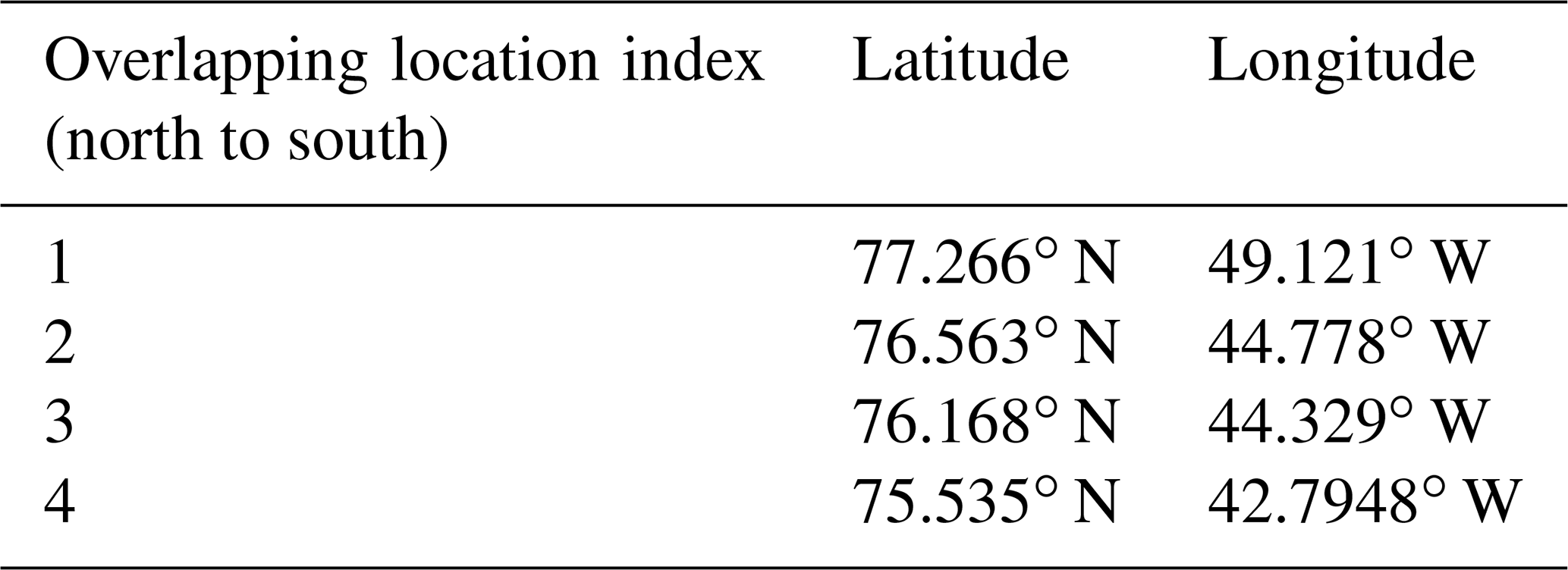
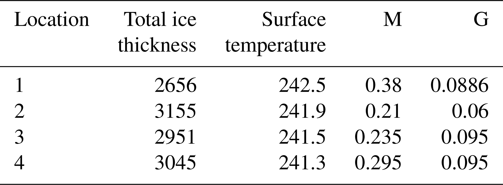
To validate the potential utility of combined active and passive measurements of firn properties, locations 1 through 4 listed in Table 1, where the snow radar and UWBRAD were nearly co-located over Greenland in 2017, were identified based on the 2017 flight paths shown in Fig. 3. X-ray tomography data near the first location were compared with the radar echo to validate the existence of refrozen layers.
Table 1Latitude and longitude for crossover locations of 2017 UWBRAD and snow radar measurements.
2.2 The Community Firn Model and in situ measurements
The locations where active and passive measurements are both available are presented in Fig. 1. Although lots of in situ measurements of the snow density are available, they are spread over a large spatial and temporal scale (Montgomery et al., 2018). Previous studies have shown that thermal emission at 0.5–2 GHz is highly influenced by the density fluctuations in the range of the centimeter scale. However, in situ measurements usually take on the scale of tens of centimeters, which does not fit the need of characterizing the density statistics on the microwave scale. Thus, to evaluate the inferred the density fluctuations from microwave sensor data, we use the modeled firn profile as a reference.
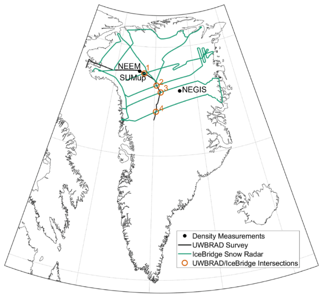
Figure 1Flight paths of UWBRAD and the snow radar in 2017. SUMup: Surface Mass Balance and Snow on Sea Ice Working Group.
We use the Community Firn Model v1.1.6 (CFM; Stevens et al., 2020) to simulate the firn column density profile at several locations across the ice sheet. The CFM was built as a resource for the glaciology community and consists of a modular, open-source framework for Lagrangian modeling of several firn and firn–air-related processes (Stevens et al., 2020). CFM simulations are set up as detailed in Medley et al. (2022), where the model is forced by a modified version of the MERRA-2 (Modern-Era Retrospective analysis for Research and Applications) global atmospheric reanalysis (Gelaro et al., 2017) at 5 d temporal resolution. The only difference between the CFM simulations from Medley et al. (2022) and those presented here is that a time-varying initial density ρ0 of the firn column is introduced using the parameterization in Fausto et al. (2018): , where Ta is the atmospheric temperature (in °C) at each time step. When comparing CFM-generated density profiles with observations, we use the simulated profile that is most contemporaneous with the observations. For a detailed description of the CFM setup, see Medley et al., 2022. The vertical density profile of the firn can be characterized by , where ρm(z) is a mean profile that gradually increases with depth and ρf(z) is a fluctuating profile which fluctuates around ρm(z) and is characterized by standard deviation Δρ(z) and correlation length lz(z).
We selected three locations to compare in situ measurements and CFM simulations. The first profile was collected at T41 (71.08° N, 37.92° W) along the EGIG (Expéditions Glaciologiques Internationales au Groenland) line by Morris and Wingham (2011) in 2004 using a neutron probe. Data were collected up to 13 m below the surface at a vertical resolution of 1 cm and clearly show significant fluctuations in density in the upper firn. The second and third profiles are from a 2009 borehole measurement at the NEEM site (Baker, 2012) with a vertical resolution of ∼ 90 cm and from a 2012 measurement at the NEGIS (Northeast Greenland Ice Stream; Vallelonga et al., 2016, 2014) site having ∼ 1 m increments. The goal is to evaluate whether the CFM simulation can provide a density fluctuation and a mean profile that are physical compared to the real world.
2.3 Analytical partially coherent model
To interpret the brightness temperature, an analytical partially coherent model is implemented. An illustration of the ice sheet thermal-emission problem is shown in Fig. 2. A firn layer of thickness d1 (location 1) exists near the ice sheet surface. The density of the firn layer is modeled as with ρm(z) as the mean density profile. Due to the great melt events starting in 2012, refrozen high-density layers appear in the region, which is typically considered a dry zone. The effects of these layers are also considered. The fluctuating profile is described as . Notice that the fluctuating profile varies in three dimensions and has two scales, short (ρfs) and long (ρfl). The real and imaginary parts of the microwave permittivity of the firn are related to the firn density using the models in Matzler (1996) and Tiuri et al. (1984). The correlation function for each scale of the fluctuating density is described by
in which Δεrf(z) is the standard deviation, lz(z) is the permittivity vertical correlation length, and lρ is the horizontal correlation length. The correlation function is described as having a Gaussian form laterally and an exponential form vertically based on the model used in Tsang et al. (2000). The exponential form for the vertical correlation function is adopted based on analyses showing similar properties for the firn density itself (Tsang et al., 2000). Both Δεrf(z) and lz are modeled as functions of depth due to the compaction of the firn, while lρ is modeled as independent of depth.
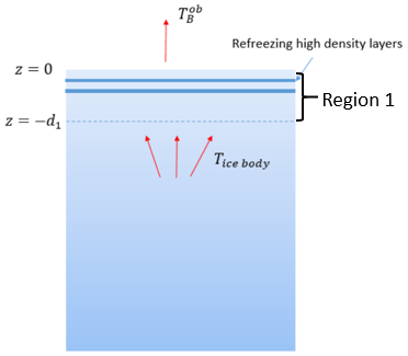
Below location 1, the main ice body can be multiple kilometers thick with a temperature profile that varies in depth. Thermal emission from the main ice body is calculated using the existing partially coherent model (Tan et al., 2021) and the temperature profile obtained in Yardim et al. (2022). The temperature in location 1 is modeled as a constant value T0. Although the top 10–20 m of firn experiences seasonal temperature changes, these variations have little effect on brightness temperatures at frequencies less than 2 GHz due to the limited emission directly from the firn layer.
Applying the radiative transfer theory of microwave emission and scattering, the upward- and downward-propagating specific intensities Iu and Id in location 1 satisfy
with the boundary conditions
In the above equations, Iu and Id are 2 × 1 vectors in which the upper row is for vertical polarization and the lower row is for horizontal polarization. κa(z) is the absorption coefficient determined by the mean density profile, while is the scattering coefficient due to the randomly fluctuating portion of the density profile. The phase matrices and couple specific intensities from other directions θ′ into the direction of interest θ in the forward- or backward-propagating hemispheres. The boundary conditions specify that the firn-to-air interface at z=0 is reflective with reflection coefficient and that the compacted firn-to-ice interface at with d1 = 100 m is not reflective. An iterative approach is then used to solve the equations. Since the permittivity variation is small, the first-order solution together with the zeroth-order solution provides sufficient accuracy. A detailed solution of the equations can be found in Appendix A. The method is partially coherent because the phase matrices are obtained using a coherent formulation of the problem of continuous medium scattering.
High-density refrozen layers are included by incorporating their additional reflections as
where accounts for the transmission from each layer, is the brightness temperature observed by the radiometer, and is the permittivity of the mean profile just below the snow–air interface. This multiplicative approach is reasonable because the microwave wavelength between 0.5 and 2 GHz is larger than the typical layer thickness.
The resulting model captures coupling between scattering in different directions and polarizations through the phase matrices and . The previous “random-layer” 1D formulation of Tan et al. (2021) captures neither of these effects.
3.1 Firn density measurements at borehole sites and the associated CFM profiles
The high-resolution profile (1 cm resolution) at T41 enables an estimation the standard deviation SD(ρ) and correlation length lz of the fluctuating profile every meter in depth (Table 2). The coarser profiles (∼ 1 m resolution) at locations 2 and 3 do not allow for such an analysis, but information on the depth at which a “critical” density (i.e., 550 kg m−3) is reached can be obtained.
In Fig. 3, the profiles from T41 high-resolution measurements and CFM simulation is plotted. The standard deviation of density and its correlation length based on every 1 m segment is provided in Table 2. Both the in situ and CFM profiles at T41 show small and fast variations superimposed on the larger but relatively slowly varying mean profile. The 1 m density standard deviations (SD(ρ)) in Table 2 for the neutron probe and CFM are comparable, with most of the values around 0.03 g cm−3. Vertical correlation lengths obtained both from the Morris and Wingham (2011) profile and the CFM simulation are < 20 cm with mean values of 14.2 and 9.4 cm, respectively. The results from the CFM are usually used to evaluate the mean firn density.
Table 2Estimated density standard deviations (SD(ρ)) and correlation lengths (lz) estimated using 1 m of data beginning at the specified depth for Summit Station, Greenland, from the neutron probe dataset of Morris and Wingham (2011) and the CFM.
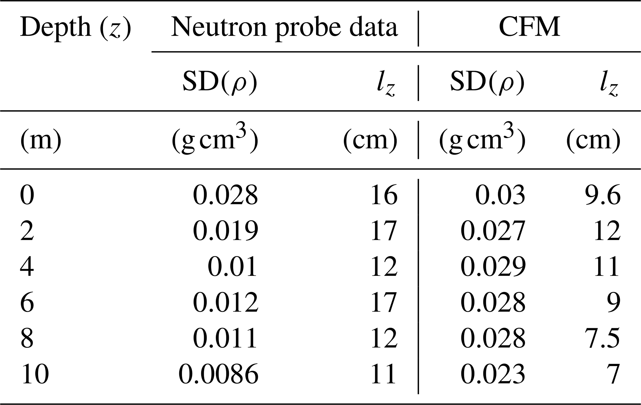
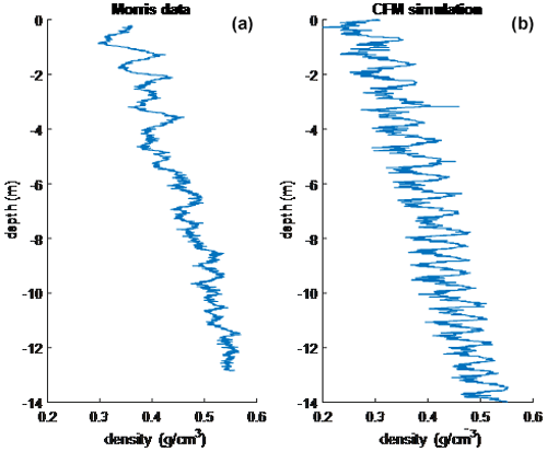
Figure 3(a) Morris and Wingham (2011) density profile measured near Summit station, Greenland, in summer 2004. (b) Corresponding CFM model simulation.
The comparison here is to show that (1) the CFM is not generating very large fluctuations (s(ρ) > mean(ρ)) since observed density profile shows an rms density of fluctuation smaller than the mean profile and (2) the simulated profile is not changing too slowly compared to the measurements. If the profile is changing too slowly (lzCMF > 2lz measured), this means that the simulated CFM profile is not able to characterize the density changes. This shows that CFM results are reasonable compared to measured data. The comparison here is performed for the statistics of the “long scale” (lz of several centimeters), which is mainly due to the yearly snowfall. The “short scale” (lz < 2 cm), even when we have seen the fluctuations in the profile, cannot be captured since the data resolution is comparable to the correlation length.
In Fig. 4, we show the ice core measurement of the NEEM (Fig. 4a) and NEGIS (Fig. 4b) sites plotted together with the mean profile generated from the CFM. We fit the ice core data with an exponential function of depth that was then extrapolated to find the depth at which the exponential function reached 550 kg m−3. The resulting depths from the NEEM and NEGIS sites and from the corresponding CFM simulations are shown in Table 3. Figure 4 shows reasonable agreement for observing the CFM-simulated mean profile plotted together with the borehole measurements. The NEEM site shows a difference of 1.8 m in the position of critical density; this is due to fitting the two stages of densities with a single exponential.
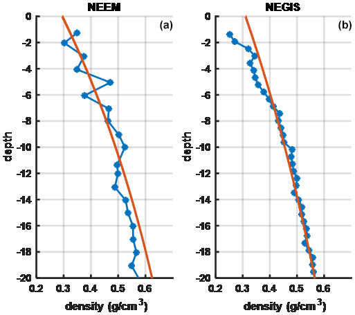
Figure 4In situ and CFM density profiles for the NEEM and NEGIS sites (blue: ice core data, orange: fitted mean profile from the CFM simulation).
Table 3Estimated depth at which the mean density profile reaches the critical density value of 550 kg m−3 for the NEEM and NEGIS sites in situ measurements and corresponding CFM simulations.
The results of this section suggest that the CFM, when run at a high time resolution, can produce firn density profiles that are in reasonable agreement with in situ measurements. The mean profiles, as shown in the comparison, are in good agreement with the measurements.
3.2 Refrozen layers in the upper-firn region
As stated earlier, the great melt events create refrozen layers in the “dry” zone of Greenland. In this section, we compare the snow radar echogram with the CFM-simulated profiles. An X-ray tomography profile near location 1 collected in 2015 (Montgomery et al., 2018) is also compared with the radar echo. Figure 5 plots three example radar echo profiles near location 1 in Fig. 1 along with an echogram showing multiple profiles versus the position along the flight path. Individual echo profiles show multiple significant backscatter peaks in the upper firn, but the echogram demonstrates that returns can fluctuate significantly from location to location. CFM profile simulations also account only for large-scale climate properties in simulating firn profiles so that a spatial average of radar measurements is also reasonable. Besides, UWBRAD measurements also correspond to a footprint of 1 km diameter. These facts validate the averaging over 1 km data.
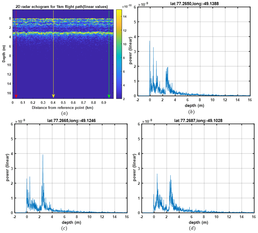
Figure 5(a) Snow radar echogram versus depth in the firn along the flight path. Three selected echo profiles from the echogram positions are denoted as (b) red, (c) yellow, and (d) green. The echogram show bright edges near the surface which can be attributed to the refrozen layers with higher dielectric contrast.
Figures 6 and 7 compare CFM-simulated density profiles for crossover locations 1–2 (Fig. 6) and 3–4 (Fig. 7) with the 1 km averaged radar echoes as a function of depth. All locations show secondary backscatter peaks at a depth of 2–2.5 m that corresponds to peaks in the CFM density profiles. These peaks have an amplitude comparable to the snow–air interface, which is likely to be caused by the refrozen layers created in the melt events starting in the year of 2012. The snow radar also observes backscatter peaks at shallower depths that do not correspond to similar density features in the simulated profiles, potentially due to inaccuracies in the climate forcing used for recent periods. Additional smaller backscatter peaks appear at 6–8 m depth that in many cases have matching CFM density peaks, but the lower level of the backscatter returns makes a direct comparison with CFM information more challenging.
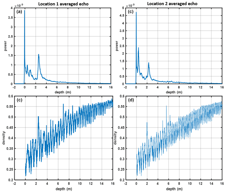
Figure 6Averaged radar echoes for crossover locations (a) 1 and (b) 2 and (c, d) corresponding CFM-simulated density profiles.
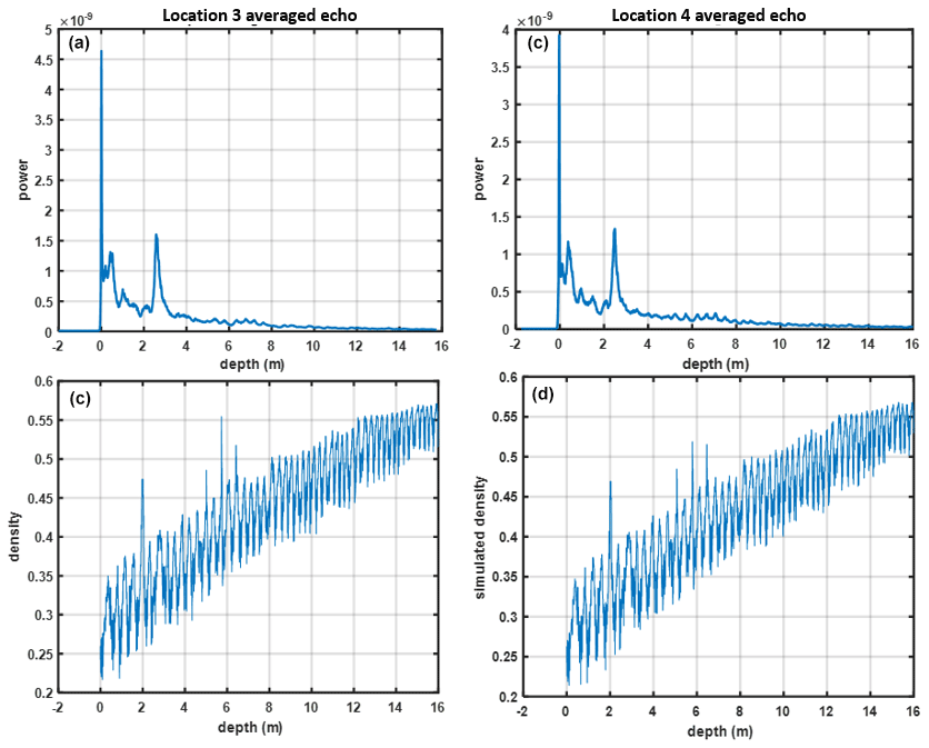
Figure 7Averaged radar echoes for crossover locations (a) 3 and (b) 4 and (c, d) corresponding CFM-simulated density profiles.
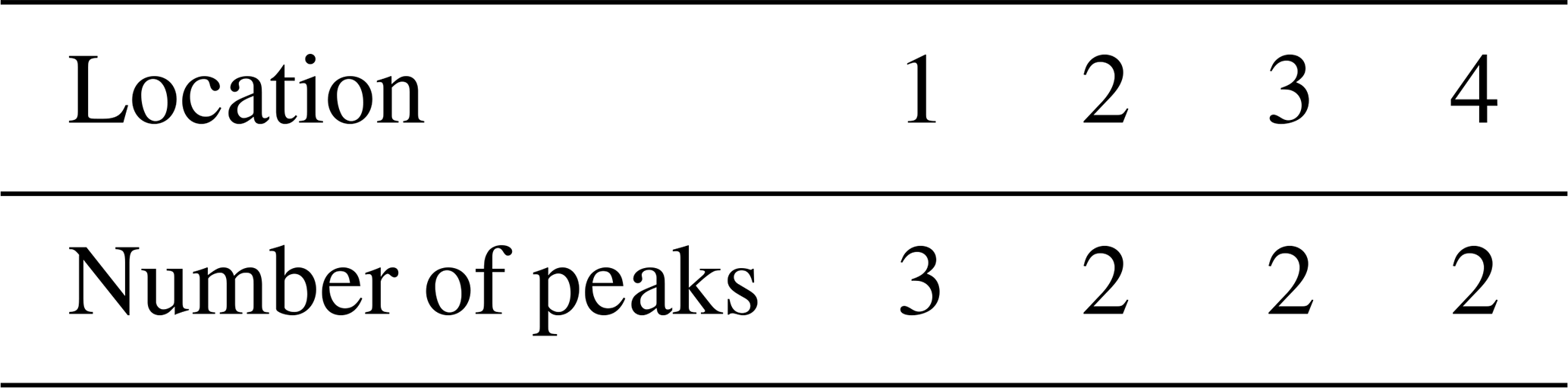
The 2015 X-ray tomography data from the Surface Mass Balance and Snow on Sea Ice Working Group (SUMup) providing a snapshot of the upper 2 m of the firn for a location near crossover location 1 are shown in Fig. 8. The X-ray profile was shifted 1 m in depth to compensate for snowfall between the 2015 tomography and 2017 radar measurements. The strong radar echo near 2.5 m depth again collocates well with X-ray density features near this depth related to the 2012 melt event. It is noted that the tomographic profile corresponds only to a single location rather than the 1 km average used in the radar echo so that the detailed features in the tomography profile are not observed in the averaged radar measurement, although similar detailed features can be identified in some individual radar echo profiles. Table 4 presents a summary of the numbers of peaks detected in the averaged snow radar echogram at each of the four crossover sites.
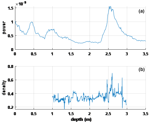
Figure 8(a) Averaged snow radar echo compared to (b) X-ray high-resolution tomography density data near crossover location 1.
The results of this section suggest that strong echoes observed by the snow radar are due to refrozen layers in the firn. CFM-simulated density peaks are shown to correspond reasonably to high-backscatter echoes, with a melt event likely having happened in the year of 2012. X-ray tomography data also show the impact of the 2012 melt event and correlate well with radar measurements (Schaller et al., 2016).
3.3 Studies of the impact of each density component on 0.5–2 GHz brightness temperatures
In this section, we use the radiative transfer model to study the frequency response of a different component in the firn. The reflection is evaluated for the long scale, short scale, and refrozen layers. The model was first applied to simulate the impact of long-scale density fluctuations on 0.5–2 GHz brightness temperatures. Figure 9 shows example reflections resulting from long-scale firn density variations at the snow–air interface, using the parameter in Table 5. The maximum and minimum of the reflection within the bandwidth is 0.126 and 0.118, a difference of 0.008. The reflection is unitless as a ratio of reflected power to incident power. The reflectivity is significant but remains approximately constant in frequency in this case.
Table 5Properties of the short-scale and long-scale variations in density and frozen layers.
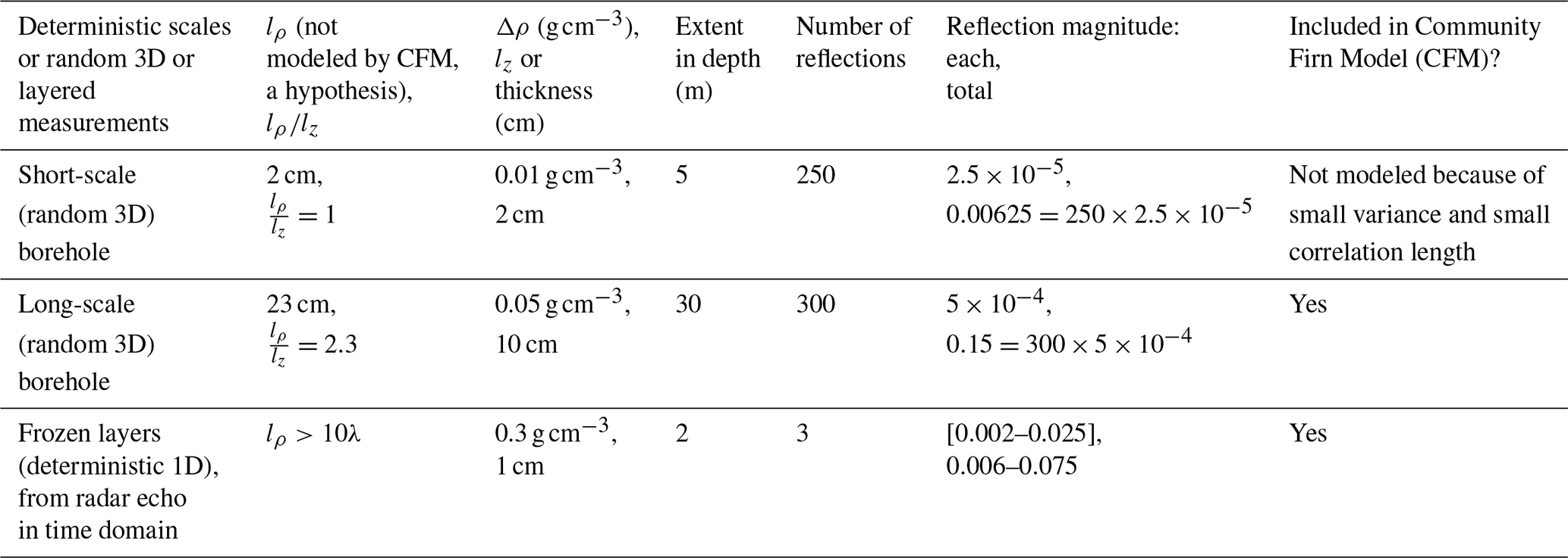
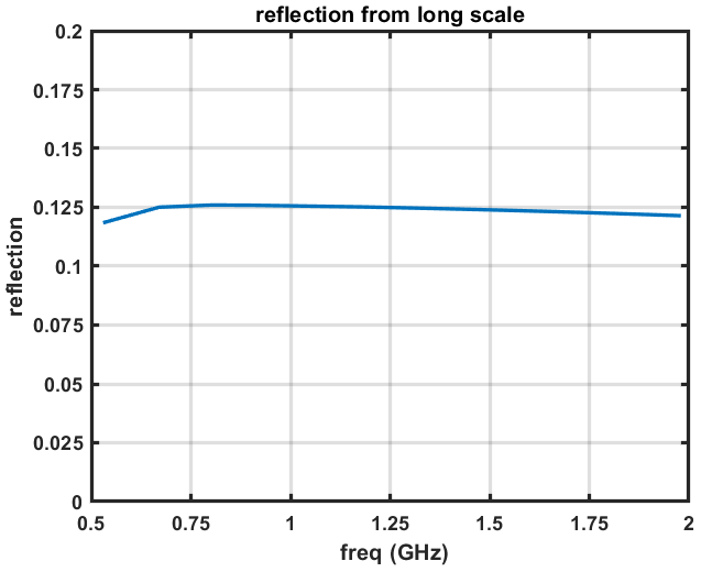
Figure 9Reflections from the long scale and snow–air interface; the results are almost constant in frequency.
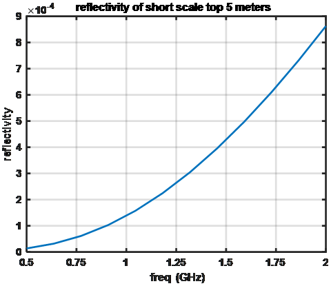
A similar study for short-scale variations using the parameters in Table 5 is presented in Fig. 10. The parameters of the SD(ρ) and lz is from the results of Tan et al. (2021). We used a small horizontal correlation length for the short scale since these kind of small variations are hard to obtain horizontally on the scale of tens of centimeters. We also assume the short scale exists in a shorter vertical range due to the densification effect. The small reflectivity values obtained suggest that the contribution of short scales is negligible compared to the long scale.
The reflectivity resulting from a single refrozen layer with a relative permittivity of 2.7 and thickness of 1 cm in a background with a relative permittivity of 1.63 is shown in Fig. 11. These results show a significant variation with frequency, ranging from 0.002 to 0.025 and from 0.5 to 2 GHz, suggesting that refrozen layers can be important contributors to the frequency variation in 0.5–2 GHz brightness temperatures. Table 5 provides a further summary of insights obtained from Figs. 9–11 and other similar simulations.
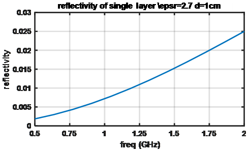
Figure 11Reflectivity of a single layer with a permittivity of 2.7 and thickness of 1 cm in a mean permittivity of ϵr=163 (0.35 g cm−3 in density).
With the understanding that the refrozen layers are contributing to the reflection change within the 0.5–2 GHz range, we now look at the UWBRAD measurements taken at the four locations in Fig. 1. Figure 12 plots UWBRAD 0.5, 1.1, and 1.8 GHz brightness temperatures at the four crossover locations. The frequency variations in brightness temperatures at location 1 (rightmost point in Fig. 12) are larger than at the other three locations, which can be related to the number of radar echo peaks at these locations (Table 4).
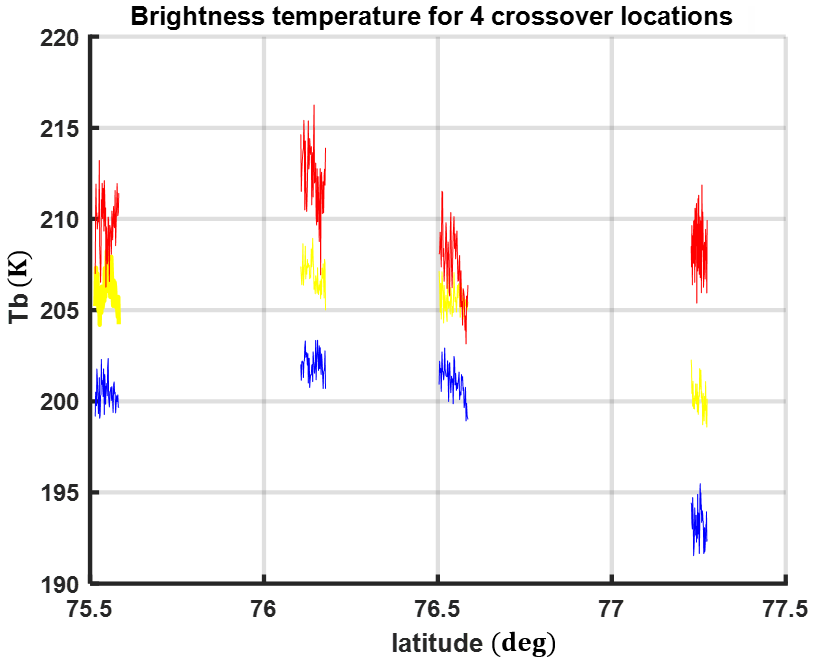
Figure 12Brightness temperature for three channels of 0.5 GHz (red), 1.1 GHz (yellow), and 1.8 GHz (blue). Crossover locations 1 to 4 are from right to left in the figure.
3.4 Comparisons of modeled and measured brightness temperatures
In this section, the analytical partially coherent model was first used to simulate UWBRAD-acquired brightness temperatures. Then the input parameters are compared with the profiles from CFM simulations.
To simulate UWBRAD brightness temperatures, temperature profiles from the NGRIP to NEEM sites retrieved in Yardim et al. (2022) (see Appendix B) are used with the partially coherent model (Tan et al., 2021) to provide the upward-going brightness temperature at depth . A mean profile of is also used for all four crossover locations based on analysis of CFM outputs for the four locations which were found to have similar mean density behaviors.
An iterative process was used to refine model parameters in order to obtain a reasonable match to the UWBRAD measurements, as shown in Fig. 13. It should be noted that UWBRAD variations at these sites can be approximately 3 K so that the agreement achieved is comparable to the measurement accuracy.
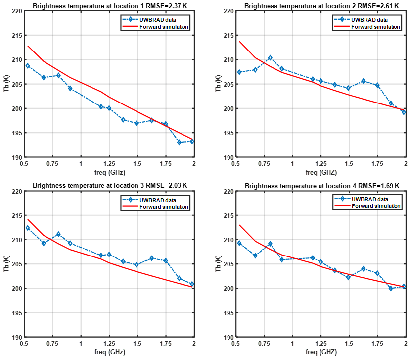
Figure 13Brightness temperature over the four overlapping positions. The simulated results are plotted together with the UWBRAD data.
Table 6 summarizes the parameters obtained; note that SD(ρ) and lz were decreased in depth through a multiplication with the functions and , respectively, where z is the depth in meters, for the large scale and with for the short scale. Numbers in the exponential functions are in terms of meters. The selection of the exponential decays for the SD(ρ) long scale is to make sure that the density fluctuations would disappear when the firn is very close to ice. For the short scale, the decay is much faster due to densification, believing the effects are negligible. A decrease in correlation length is a tuning parameter to make sure the SD(ρ) becomes 0 before lz becomes too small (). The horizontal correlation length for the long-scale variations was obtained as lρ=23 cm, which appears consistent with reports from in situ investigations and is similar to the properties of firn surface horizontal variations. The permittivity and thickness of the high-density layers used in simulating the brightness temperature are also listed in Table 6; the number of high-density layers at each site was selected based on the radar analysis in Table 4.
Table 6Parameters used in forward-modeling brightness temperature. The decrease in SD(ρ) and lz(z) follows .
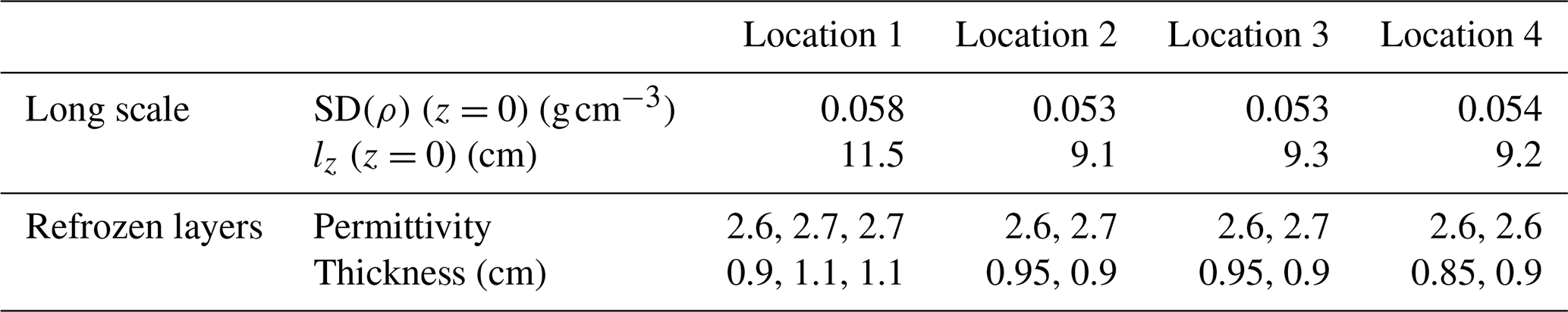
Table 7Near-surface long-scale properties from CFM simulation and accumulation rate.
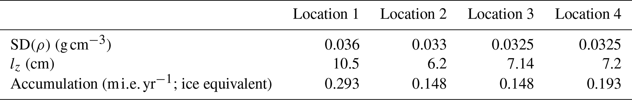
Long-scale density fluctuation parameters inferred from the CFM are listed in Table 6 for comparison. For location 1, the microwave-estimated SD(ρ) is 0.058 g cm−3 with lz = 11.5 cm, while the corresponding values for locations 2 through 4 are 0.053 g cm−3 with a correlation length of ∼ 9 cm. The CFM results show SD(ρ) values of 0.036 g cm−3 with lz = 10.5 cm for location 1 and 0.033 g cm−3 with a vertical correlation length close to 7 cm for the other locations. While the SD(ρ) used in the forward model is about 0.02 g cm−3 higher than the CFM, SD(ρ) values in both cases agree in the higher SD(ρ) and lz values at location 1. While differences in the microwave-derived and CFM-derived density fluctuation values are significant, the relative agreement achieved suggests that 0.5–2 GHz brightness temperatures can provide information on firn density fluctuations if refrozen-layer effects are accounted for using radar-derived information.
Modeling the density fluctuations with horizontal variation on the scale of wavelength enables the coupling between the emission of V- (vertically) and H-polarized (horizontally) brightness temperature. To show this effect, we compare the forward-modeling results using finite lρ and lρ=∞ with Soil Moisture and Ocean Salinity (SMOS) data collected over Dome C, Antarctica, where in situ studies have been performed (Brogioni et al., 2015; Leduc-Leballeur et al., 2015). The V- and H-polarized brightness temperature was modeled in Tan et al. (2015); however the 1D random media model could not explain the H-polarized TB. Forward model predictions were also compared with brightness temperatures at Dome C measured by the SMOS satellite. SMOS operates at 1.4 GHz and has both V and H channels. The synthetic aperture technique in SMOS make multi-angle observations possible as provided in the SMOS L1C data product. Firn properties at Dome C are very different from those in Greenland. The accumulation rate of Dome C is 0.1 m yr−1 (Brogioni et al., 2015) in contrast to the higher accumulation rates in Greenland shown in Table 7. A shorter correlation length therefore should be expected as compared to Greenland, and temporal effects on the firn will less significant compared to Greenland. Refrozen layers at this site are also neglected as significant melt events are not expected. A comparison of the firn properties used in Greenland and at Dome C is provided in Table 8 to summarize these discussions.
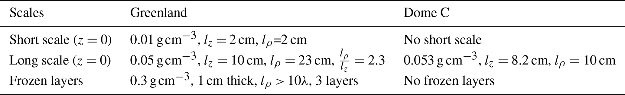
Forward model predictions of 1.4 GHz brightness temperatures versus angles are shown in Fig. 14 using lρ = 10 cm and lρ=∞, along with SMOS measurements averaged over a 10-year time period from 2011 to 2021. The SMOS error bars further indicate the expected accuracies of the SMOS data shown.
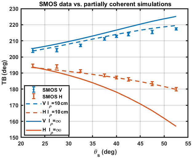
Figure 14The 10-year-averaged SMOS data compared with partially coherent forward model simulations.
In simulating the results, the density parameters at z=0 are given by Table 4. The surface density fluctuation is selected between the ground measurement data at Dome C (Brogioni et al., 2015) and the values obtained in Leduc-Leballeur et al. (2015); note that information on the density correlation length is not provided in these works. The mean profile density follows Brogioni et al. (2015), and a Robin model for temperature is used. We assume that SD(ρ) and lz have a dependence of and , respectively, to model the process of densification.
The results show that the model predictions with lρ=10 cm provide good agreement with SMOS data in the range of 22.5–52.5° incidence angle and with rms difference over an angle of 1.4 K in V and 0.8 K in H. The 1D lρ=∞ results in contrast show up to 17 K differences in the H-polarized simulations. These results show that including the effects of finite horizontal correlation length allows for the coupling between angle and polarization effects necessary to reproduce SMOS observations.
The analysis of UWBRAD data over Greenland and Dome C, Antarctica, has shown the strong effects of density fluctuations over the brightness temperature in the L band. This shows that passive microwaves can be used as a tool to infer the density fluctuations remotely. Previously, density properties could only be obtained by in situ measurements (e.g., snow pit), which can only be taken over several places for a given period of time in a year. Characterizing the density fluctuation change can help characterize the mass balance of firn given that the elevation change in firn can be due to the density change.
The radiative transfer model developed here can also be used to analyze the time series brightness temperature over the regions where a perennial firn aquifer exists. Resolution-enhanced time series brightness temperature collected by SMAP (Soil Moisture Active Passive) over these regions has shown an exponential-like pattern from the end of the melting season to the early spring of the next year (Miller et al., 2020, 2012). Physical modeling work for the V and H TB data from SMAP has been performed by Bringer et al. (2017), but the forward-modeled results show a much larger TB difference in the V and H channels. Based on the model in this paper, we can try to better interpret the SMAP observations physically.
As in the previous studies, density fluctuations have also affected the retrieval of temperature profiles of the ice sheet. The retrieval can be improved by knowing the density better.
The results of the paper suggest a combined active and passive method for sensing long-scale fluctuations in the firn density. These fluctuations contain information on accumulation and densification within the firn. The Community Firn Model was used to generate profiles for comparison and was shown to produce simulated profiles having reasonable agreement with in situ measurements provided that appropriate high-resolution forcing data were available. Snow radar echo measurements were shown to provide information on refrozen layers within the firn that could then be accounted for in analyzing 0.5–2 GHz brightness temperature datasets. The analytical partially coherent model reported was found to provide reasonable agreement with measured 0.5–2 GHz brightness temperatures by including the effects of refrozen layers and long-scale density fluctuations. Comparisons with SMOS measurements at Dome C in particular demonstrate the coupling between H and V polarizations that is captured by the continuous random medium description used in the model. This work shows that the co-located active and passive microwave data can be used to infer the polar firn properties that can further be compared with predictions of the CFM.
In this appendix, we give the details of the first-order solution of radiative transfer equations with a varying mean and fluctuating profile. The density profile is defined by
where ρm(z) is the mean profile which increases as the depth increases, ρf(z) is the fluctuating profile with the standard deviation SD(ρf)(z), and vertical correlation length lz(z) decreases as z decreases. The radiative transfer equations for the density fluctuating region are given as
and
The boundary conditions are given as the following:
and
The intensity vectors contain the first and second components of the Stokes vector. In the region we consider, which is tens of meters below the surface, the physical temperature of the firn is almost a constant number of T0.
The expressions for the phase functions can be found in Tsang et al. (2000). To find the solution, we multiply with the equation of upward-going intensity and integrate the equation from to . After some math manipulations, we have the expressions for upward intensity as
For the downward intensity, we multiply the downward equation with and integrate from to . The downward intensity is then obtained as
The zeroth-order solution for the upward and downward intensities is given as
and
The first-order solution of the upward intensity is given as
The specific intensity at z=0 is then given as
The Morris and Wingham (2011) density data can be provided upon request. UWBRAD data can be accessed from the UWBRAD website http://www2.ece.ohio-state.edu/~johnson/uwbrad.html (Johnson, 2017).
HX performed the majority of this work. BM provided all the simulations of density profiles and the map showing data positions over Greenland. LT advised on the modeling. JTJ and KCJ provided UWBRAD data and valuable comments on the paper. MB and LK provide the SMOS data over Dome C and suggested the usage of data.
The contact author has declared that none of the authors has any competing interests.
Publisher's note: Copernicus Publications remains neutral with regard to jurisdictional claims in published maps and institutional affiliations.
The authors would like to thank the editor, anonymous reviewers, language editor, and typesetters for their efforts on reviewing and editing the paper.
This research has been supported by the National Aeronautics and Space Administration (grant no. 80NSSC21K1062).
This paper was edited by Ruth Mottram and reviewed by two anonymous referees.
Andrews, M., Li, H., Johnson, J. T., Jezek, K. C., Bringer, A., Yardim, C., Chen, C. C., Belgiovane, D., Leuski, V., Durand, M., Duan, Y., Macelloni, G., Brogioni, M., Tan, S., and Tsang, L.: The Ultra-Wideband Software Defined Microwave Radiometer (UWBRAD) for Ice sheet subsurface temperature sensing: Calibration and campaign results, 2017 IEEE International Geoscience and Remote Sensing Symposium (IGARSS), Fort Worth, TX, USA, 23–28 July 2017, IEEE, 237–240, https://doi.org/10.1109/IGARSS.2017.8126938, 2017.
Baker, I.: NEEM Firn Core 2009S2 Density and Permeability: https://arcticdata.io/catalog/view/doi:10.18739/A2Q88G (last access: July 2012), 2012.
Bringer, A., Miller, J., Johnson, J. T., and Jezek, K. C.: Radiative transfer modelking of the brightness temperature signatures of firn aquifers, American Geophysical Union Fall Meeting, New Orleans, LA, USA, https://agu.confex.com/agu/fm17/meetingapp.cgi/Paper/283159 (last access: July 2023), 11–15 December 2017.
Brogioni, M., Macelloni, G., Montomoli, F., and Jezek, K. C.: Simulating Multifrequency Ground-Based Radiometric Measurements at Dome C—Antarctica, IEEE J. Sel. Top. Appl., 8, 4405–4417, https://doi.org/10.1109/JSTARS.2015.2427512, 2015.
Brucker, L., Picard, G., and Fily, M.: Snow grain-size profiles deduced from microwave snow emissivities in Antarctica, J. Glaciol., 56, 514–526, https://doi.org/10.3189/002214310792447806, 2010.
Champollion, N., Picard, G., Arnaud, L., Lefebvre, E., and Fily, M.: Hoar crystal development and disappearance at Dome C, Antarctica: observation by near-infrared photography and passive microwave satellite, The Cryosphere, 7, 1247–1262, https://doi.org/10.5194/tc-7-1247-2013, 2013.
CReSIS: Snow radar Data, Lawrence, Kansas, USA, Digital Media, University of Kansas, http://data.cresis.ku.edu/ (last access: July 2022), 2021.
Dattler, M. E., Lenaerts, J. T., and Medley, B.: Significant Spatial Variability in Radar-Derived West Antarctic Accumulation Linked to Surface Winds and Topography, Geophys. Res. Lett., 46, 13126–13134, https://doi.org/10.1029/2019GL085363, 2019.
Fausto, R. S., Box, J. E., Vandecrux, B., Van As, D., Steffen, K., MacFerrin, M. J., Machguth, H., Colgan, W., Koenig, L. S., McGrath, D. Charalampidis, C., and Braithwaite, R. J.: A snow density dataset for improving surface boundary conditions in Greenland ice sheet firn modeling, Front. Earth Sci., 6, 51, https://doi.org/10.3389/feart.2018.00051, 2018.
Gelaro, R., McCarty, W., Suárez, M. J., Todling, R., Molod, A., Takacs, L., Randles, C. A., Darmenov, A., Bosilovich, M. G., Reichle, R., Wargan, K., Coy, L., Cullather, R., Koster, R., Luccheis, R., Merkova, D., Nielsen, J. E., Partyka, G., Pawson, S., Putman, W., Rienecker, M., Schuber, S. D., Sienkiewicz, M., and Zhao, B.: The modern-era retrospective analysis for research and applications, version 2 (MERRA-2), J. Climate, 30, 5419–5454, https://doi.org/10.1175/JCLI-D-16-0758.1, 2017.
Jezek, K. C., Gogineni, P., and Shanableh, M.: Radar Measurements of Melt Zones on the Greenland Ice Sheet, Geophys. Res. Lett., 21, 33–36, https://doi.org/10.1029/93GL03377, 1994.
Jezek, K. C., Johnson, J. T., Drinkwater, M. R., Macelloni, G., Tsang, L., Aksoy, M., and Durand, M.: Radiometric Approach for Estimating Relative Changes in Intraglacier Average Temperature, IEEE T. Geosci. Remote, 53, 134–143, https://doi.org/10.1109/TGRS.2014.2319265, 2015.
Jezek, K. C., Johnson, J. T., Tan, S., Tsang, L., Andrews, M. J., Brogioni, M., Macelloni, G., Durand, M., Chen, C. C., Belgiovane, D. J., Duan, Y., Yardim, C., Li, H., Bringer, A., and Aksoy, M.: 500–2000-MHz Brightness Temperature Spectra of the Northwestern Greenland Ice Sheet, IEEE T. Geosci. Remote, 56, 1485–1496, https://doi.org/10.1109/TGRS.2017.2764381, 2018.
Johnson, J. T.: Ultra-Wideband Software Defined Microwave Radiometer (UWBRAD) Data over Greenland 2017, http://www2.ece.ohio-state.edu/~johnson/uwbrad.html (last access: July 2023), 2017.
Koenig, L. S., Steig, E. J., Winebrenner, D. P., and Shuman, C. A.: A link between microwave extinction length, firn thermal diffusivity, and accumulation rate in West Antarctica, J. Geophys. Res., 112, F03018, https://doi.org/10.1029/2006JF000716, 2007.
Koenig, L. S., Ivanoff, A., Alexander, P. M., MacGregor, J. A., Fettweis, X., Panzer, B., Paden, J. D., Forster, R. R., Das, I., McConnell, J. R., Tedesco, M., Leuschen, C., and Gogineni, P.: Annual Greenland accumulation rates (2009–2012) from airborne snow radar, The Cryosphere, 10, 1739–1752, https://doi.org/10.5194/tc-10-1739-2016, 2016.
Kuipers Munneke, P., Ligtenberg, S. R. M., Noël, B. P. Y., Howat, I. M., Box, J. E., Mosley-Thompson, E., McConnell, J. R., Steffen, K., Harper, J. T., Das, S. B., and van den Broeke, M. R.: Elevation change of the Greenland Ice Sheet due to surface mass balance and firn processes, 1960–2014, The Cryosphere, 9, 2009–2025, https://doi.org/10.5194/tc-9-2009-2015, 2015.
Leduc-Leballeur, M. Picard, G., Mialon, A., Arnaud, L., Lefebvre, E., Possenti, P., and Kerr, Y.: Modeling L-Band Brightness Temperature at Dome C in Antarctica and Comparison With SMOS Observations, IEEE T. Geosci. Remote, 53, 4022–4032, https://doi.org/10.1109/TGRS.2015.2388790, 2015.
Lewis, C. and Gognineni, P.: Airborne UHF radar for fine resolution mapping of near surface accumulation layers in Greenland and West Antarctica, M. S. thesis, Dept. Elect. Eng. Comput. Sci., Univ. Kansas, Lawrence, KS, USA, 158 pp., http://hdl.handle.net/1808/7008 (last access: July 2022), 2010.
Li, J. and Zwally, H. J.: Modeling of firn compaction for estimating ice-sheet mass change from observed ice-sheet elevation change, Ann. Glaciol., 52, 1–7, https://doi.org/10.3189/172756411799096321, 2011.
Ligtenberg, S. R. M., Helsen, M. M., and van den Broeke, M. R.: An improved semi-empirical model for the densification of Antarctic firn, The Cryosphere, 5, 809–819, https://doi.org/10.5194/tc-5-809-2011, 2011.
Matzler, C.: Microwave permittivity of dry snow, IEEE T. Geosci. Remote, 34, 573–581, https://doi.org/10.1109/36.485133, 1996.
Medley, B., Joughin, I., Das, S. B., Steig, E. J., Conway, H., Gogineni, S., Criscitiello, A. S., McConnel, R., Smith, B. E., van den Broeke, M. R., Lenaerts, J. T., Bromwich, D. H., and Nicolas, J. P.: Airborne-radar and ice-core observations of annual snow accumulation over Thwaites Glacier, West Antarctica confirm the spatiotemporal variability of global and regional atmospheric models, Geophys. Res. Lett., 40, 3649–3654, https://doi.org/10.1002/grl.50706, 2013.
Medley, B., Joughin, I., Smith, B. E., Das, S. B., Steig, E. J., Conway, H., Gogineni, S., Lewis, C., Criscitiello, A. S., McConnell, J. R., van den Broeke, M. R., Lenaerts, J. T. M., Bromwich, D. H., Nicolas, J. P., and Leuschen, C.: Constraining the recent mass balance of Pine Island and Thwaites glaciers, West Antarctica, with airborne observations of snow accumulation, The Cryosphere, 8, 1375–1392, https://doi.org/10.5194/tc-8-1375-2014, 2014.
Medley, B., Ligtenberg, S. R. M., Joughin, I., Van den Broeke, M. R., Gogineni, S., and Nowicki, S.: Antarctic firn compaction rates from repeat-track airborne radar data: I. Methods, Ann. Glaciol., 56, 155–166, https://doi.org/10.3189/2015AoG70A203, 2015.
Medley, B., Neumann, T. A., Zwally, H. J., Smith, B. E., and Stevens, C. M.: Simulations of firn processes over the Greenland and Antarctic ice sheets: 1980–2021, The Cryosphere, 16, 3971–4011, https://doi.org/10.5194/tc-16-3971-2022, 2022.
Miller, J. Z., Long, D. G., Jezek, K. C., Johnson, J. T., Brodzik, M. J., Shuman, C. A., Koenig, L. S., and Scambos, T. A.: Brief communication: Mapping Greenland's perennial firn aquifers using enhanced-resolution L-band brightness temperature image time series, The Cryosphere, 14, 2809–2817, https://doi.org/10.5194/tc-14-2809-2020, 2020.
Miller, J. Z., Culberg, R., Long, D. G., Shuman, C. A., Schroeder, D. M., and Brodzik, M. J.: An empirical algorithm to map perennial firn aquifers and ice slabs within the Greenland Ice Sheet using satellite L-band microwave radiometry, The Cryosphere, 16, 103–125, https://doi.org/10.5194/tc-16-103-2022, 2022.
Montgomery, L., Koenig, L., and Alexander, P.: The SUMup dataset: compiled measurements of surface mass balance components over ice sheets and sea ice with analysis over Greenland, Earth Syst. Sci. Data, 10, 1959–1985, https://doi.org/10.5194/essd-10-1959-2018, 2018.
Morris, E. M. and Wingham, D. J.: The effect of fluctuations in surface density, accumulation and compaction on elevation change rates along the EGIG line, central Greenland, J. Glaciol., 57, 416–430, https://doi.org/10.3189/002214311796905613, 2011.
Panzer, B., Leuschen, C., Patel, A., Markus, T., and Gogineni, S.: Ultra-wideband radar measurements of snow thickness over sea ice, 2010 IEEE International Geoscience and Remote Sensing Symposium, Honolulu, HI, USA, 25–30 July 2010, 3130–3133, https://doi.org/10.1109/IGARSS.2010.5654342, 2010.
Schaller, C. F., Freitag, J., Kipfstuhl, S., Laepple, T., Steen-Larsen, H. C., and Eisen, O.: A representative density profile of the North Greenland snowpack, The Cryosphere, 10, 1991–2002, https://doi.org/10.5194/tc-10-1991-2016, 2016.
Shepherd, A., Gilbert, L., Muir, A. S., Konrad, H., McMillan, M., Slater, T., Briggs, K. H., Sundal, A. V., Hogg, A. E., and Engdahl, M. E.: Trends in Antarctic Ice Sheet elevation and mass, Geophys. Res. Lett., 46, 8174–8183, https://doi.org/10.1029/2019GL082182, 2019.
Smith, B., Fricker, H. A., Gardner, A. S., Medley, B., Nilsson, J., Paolo, F. S., Holschuh, N., Adusumilli, S., Brunt, K., Csatho, B., Harbeck, K., Markus, T., Neumann, T., Siegfried, M. R., and Zwally, H. J.: Pervasive ice sheet mass loss reflects competing ocean and atmosphere processes, Science, 368, 1239–1242, https://doi.org/10.1126/science.aaz5845, 2020.
Stevens, C. M., Verjans, V., Lundin, J. M. D., Kahle, E. C., Horlings, A. N., Horlings, B. I., and Waddington, E. D.: The Community Firn Model (CFM) v1.0, Geosci. Model Dev., 13, 4355–4377, https://doi.org/10.5194/gmd-13-4355-2020, 2020.
Stevens, M., Vo, H., emmakahle, and Jboat: UWGlaciology/CommunityFirnModel: Version 1.1.6, Zenodo [code], https://doi.org/10.5281/zenodo.5719748, 2021.
Tan, S., Aksoy, M., Brogioni, M., Macelloni, G., Durand, M., Jezek, K. C., Wang, T.-L, Tsang, L., Johnson, J. T., Drinkwater, M. R., and Brucker, L.: Physical Models of Layered Polar Firn Brightness Temperatures From 0.5 to 2 GHz, IEEE J. Sel. Top. Appl. 8, 3681–3691, https://doi.org/10.1109/JSTARS.2015.2403286, 2015.
Tan, S., Tsang, L., Xu, H., Johnson, J. T., Jezek, K. C., Yardim, C., Durand, M., and Duan, Y.: A Partially Coherent Approach for Modeling Polar Ice Sheet 0.5–2-GHz Thermal Emission, IEEE T. Geosci. Remote, 59, 8062–8072, https://doi.org/10.1109/TGRS.2020.3039057, 2021.
Tiuri, M., Sihvola, A., Nyfors, E., and Hallikaiken, M.: The complex dielectric constant of snow at microwave frequencies, IEEE J. Oceanic Eng., 9, 377–382, https://doi.org/10.1109/JOE.1984.1145645, 1984.
Tsang, L., Kong, J. A., and Ding, K. H.: Scattering of Electromagnetic Waves, 1: Theory and Applications, Wiley Interscience, 426 pp., ISBN 0-471-38799-7, 2000.
Vallelonga, P.: Northeast Greenland Ice Stream (NEGIS) 2012 Ice 110 Core Chemistry and Density, NOAA, https://www1.ncdc.noaa.gov/pub/data/paleo/icecore/greenland/negis2012dens.txt (last access: July 2022), 2016.
Vallelonga, P., Christianson, K., Alley, R. B., Anandakrishnan, S., Christian, J. E. M., Dahl-Jensen, D., Gkinis, V., Holme, C., Jacobel, R. W., Karlsson, N. B., Keisling, B. A., Kipfstuhl, S., Kjær, H. A., Kristensen, M. E. L., Muto, A., Peters, L. E., Popp, T., Riverman, K. L., Svensson, A. M., Tibuleac, C., Vinther, B. M., Weng, Y., and Winstrup, M.: Initial results from geophysical surveys and shallow coring of the Northeast Greenland Ice Stream (NEGIS), The Cryosphere, 8, 1275–1287, https://doi.org/10.5194/tc-8-1275-2014, 2014.
Yardim, C., Johnson, J. T., Jezk, K. C., Andrews, M. J., Durand, M., Duan, Y., Tan, S., Tsang, L., Brogioni, M., Macelloni, G., and Bringer, A.: Greenland Ice Sheet Subsurface Temperature Estimation Using Ultrawideband Microwave Radiometry, IEEE T. Geosci. Remote, 60, 1–12, 4300312, https://doi.org/10.1109/TGRS.2020.3043954, 2022.
Zabel, I. H. H., Jezek, K. C., Baggeroer, P. A., and Gogineni, S. P.: Radar Observations of Snow Stratigraphy and Melt Processes on the Greenland Ice Sheet, Ann. Glaciol., 21, 40–44, https://doi.org/10.3189/S0260305500015573, 1995.
- Abstract
- Introduction
- Method
- Results
- Discussion
- Conclusions
- Appendix A: First-order iterative approach for firn emission
- Appendix B: Robin model parameters for the four locations
- Data availability
- Author contributions
- Competing interests
- Disclaimer
- Acknowledgements
- Financial support
- Review statement
- References