Basal melt rates and ocean circulation under the Ryder Glacier ice tongue and their response to climate warming: a high-resolution modelling study

The oceanic forcing of basal melt under floating ice shelves in Greenland and Antarctica is one of the major sources of uncertainty in climate ice sheet modelling. We use a high-resolution, nonhydrostatic configuration of the Massachusetts Institute of Technology general circulation model (MITgcm) to investigate basal melt rates and melt-driven circulation in the Sherard Osborn Fjord under the floating tongue of Ryder Glacier, northwestern Greenland. The control model configuration, based on the first-ever observational survey by Ryder 2019 Expedition, yielded melt rates consistent with independent satellite estimates. A protocol of model sensitivity experiments quantified the response to oceanic thermal forcing due to warming Atlantic Water and to the buoyancy input from the subglacial discharge of surface fresh water. We found that the average basal melt rates show a nonlinear response to oceanic forcing in the lower range of ocean temperatures, while the response becomes indistinguishable from linear for higher ocean temperatures, which unifies the results from previous modelling studies of other marine-terminating glaciers. The melt rate response to subglacial discharge is sublinear, consistent with other studies. The melt rates and circulation below the ice tongue exhibit a spatial pattern that is determined by the ambient density stratification.

1 Introduction

Increasing ice mass losses from the Greenland Ice Sheet and Antarctic Ice Sheet result from atmosphere–cryosphere–ocean interactions, which involve a range of processes including surface ice melt, internal ice dynamics and ocean-driven basal melt, wind, tides and sea ice, often coupled in a nonlinear way (Holland et al., 2008a; Straneo et al., 2012; Smith et al., 2020; Slater and Straneo, 2022). Freshwater flux from the melting ice sheets into the ocean leads to a global sea level rise and local impacts on coastal communities worldwide, and the observed acceleration of the ice sheet melt has been attributed to anthropogenic climate change (Fox-Kemper et al., 2021). A large community effort has thus been put forward to observe, quantify and understand the underlying processes and to develop representations (parameterizations) of the ice melt processes in climate models to improve the projections of future ice sheet mass loss and its impacts (Asay-Davis et al., 2017; Edwards et al., 2014; Cowton et al., 2015; Lazeroms et al., 2018; Sheperd and Nowicki, 2017; Nowicki and Seroussi, 2018; Pelle et al., 2019). This task is far from simple as the processes involved often feature small scales and complex geometries of both ice and ocean domains and their interaction with the atmosphere.

The Greenland Ice Sheet (GrIS) holds about 7 m of sea level equivalent. It contributed +13.5 mm to the global sea level rise in the period 1992–2020, according to the most recent IPCC Report (AR6, Fox-Kemper et al., 2021). During this time there is evidence that the GrIS mass loss has accelerated in recent years (1995–2012) compared with the earlier period (Enderlin et al., 2014; Hill et al., 2018). The IPCC Report estimates a 6-fold increase in mass loss rate in these last 3 decades from an average of 39 Gt yr⁻¹ in the period 1992–1999 to 243 Gt yr⁻¹ over the period 2010–2019 and projects the GrIS to likely contribute with 90–180 mm to sea level rise until 2100, while the Antarctic Ice Sheet contributes 30–340 mm (Fox-Kemper et al., 2021, SSP5-8.5). Ice mass loss from GrIS has a significant local fingerprint on several densely populated coastal regions worldwide (Rietbroek et al., 2016). Furthermore, freshwater input from the melting GrIS into the ocean has a potentially substantial (yet poorly quantified, and vividly debated) impact on freshwater budget and dense water formation in the subpolar North Atlantic and hence on the strength and stability of the large-scale thermohaline circulation (Rahmstorf et al., 2015; Boning et al., 2016; Luo et al., 2016; Rhein et al., 2018; Swingedouw et al., 2022).

The GrIS marine-terminating glaciers drain into long and narrow fjords that connect to the open ocean. The fjords are stratified with a deeper layer of warm and saline Atlantic Water (AW), overlaid by a colder and fresher Polar Water (PW) of Arctic origin (Straneo et al., 2012). The AW enters the Nordic Seas as an upper layer of the Norwegian Atlantic Current and undergoes deepening and cooling under its poleward pathway; upon reaching the Fram Strait the AW flow bifurcates into one branch recirculating cyclonically in the Nordic Seas and the Labrador Sea, and the other one taking a detour around the Arctic Ocean (Mauritzen et al., 2011; Koszalka et al., 2013; Rudels et al., 2015). The temperature and salinity properties of AW reaching the glacial fjords around Greenland vary thus regionally. The AW that reaches the northern coast of Greenland had circulated around the Arctic Ocean and is therefore the coldest variant of AW reaching the GrIS (Straneo et al., 2012). The exposure to thermal oceanic forcing (temperature difference between the ocean water and the ice) varies therefore regionally around Greenland in addition to local differences due to wind forcing, sea ice, the mesoscale circulation on the Greenland shelf and the fjord geometry (Seale et al., 2011; Rignot et al., 2012; Enderlin and Howat, 2013; Sciascia et al., 2013; Straneo and Cenedese, 2015; Gelderloos et al., 2017; Schaffer et al., 2017; Jakobsson et al., 2020; Wood et al., 2021).

The interaction at the glacier–ocean interface leading to a freshwater flux from the GrIS is realized through three different processes: basal melting of the submerged glacial ice, subglacial discharge (SGD) of the surface meltwater (the freshwater melting at the surface ice sheet due to atmospheric forcing and percolating down through the ice and toward the ice base) during the summer, and calving of icebergs at the ice front (Straneo and Cenedese, 2015). The respective importance of the processes is dependent on the timescale and the shape of the glacier terminus. The majority of glaciers in southern Greenland terminate as grounded, vertical ice fronts (Hill et al., 2018). These so-called tidewater glaciers feature fast-rising buoyant plumes because of the steepness of the ice at the terminus (Rignot et al., 2010; Xu et al., 2012; Sciascia et al., 2013) and frequent iceberg discharge through calving. They are also subject to a relatively strong seasonal forcing due to the SGD (Sciascia et al., 2014; Straneo and Cenedese, 2015).

A different type of ice–ocean interaction occurs for ice shelves, i.e. the glaciers with ice tongues, found in the north of Greenland, including the Zachariae Isstrom (ZI), the Nioghalvfjerdsfjorden, or 79^∘–North Glacier (79NG), the Ryder Glacier (RG) and the Petermann Glacier (PG). Under certain conditions, floating ice tongues can stabilize these glaciers by changing the stress balance and reducing the ice discharge across their grounding lines, an effect known as buttressing (Gudmundsson, 2013). On the other hand, due to the horizontal extent of the ice base, the area exposed to basal melting is much larger at ice shelves than it is at tidewater glaciers. The observed significant inter-annual variability in the grounding line position of 79NG and the observed and modelled retreat of ZI and PG have been attributed to oceanic forcing (Wilson and Straneo, 2015; Mayer, 2018; Choi et al., 2017; Cai et al., 2017). However, due to remoteness and logistic difficulties with the measurements, the GrIS ice shelves and their fjord outlets are still sparsely observed with regards to the ocean-driven basal melt processes.

The basal melt beneath the glacier ice tongue acts as a buoyancy source, driving a rising buoyant plume that forms an outflow of glacially modified water at its neutral density level. The entrainment into the plume drives an inflow of AW towards the ice base, establishing an estuarine circulation (Straneo and Cenedese, 2015). The basal melt processes beneath ice shelves have mostly been studied in the context of Antarctic ice shelves and have been represented in terms of a basal melt parameterization combining the basic thermodynamic considerations, conservation laws and buoyant plume dynamics and showing a good agreement with observations (e.g. Holland et al., 2008b; Jenkins, 1991, 2011; Jenkins et al., 2010; Reese et al., 2018). This has guided attempts to develop generalized versions applicable in climate models (Asay-Davis et al., 2016; Lazeroms et al., 2018; Pelle et al., 2019). However, questions remain regarding the applicability of this parameterization. One issue considers dependency of the melt on changing ambient ocean temperatures. In theory, the melt rate is linearly dependent on the thermal forcing and the boundary layer velocity, which is also linearly dependent on the thermal forcing through the buoyancy input from the melt (e.g. Holland et al., 2008b; Jenkins, 2011; Lazeroms et al., 2018), combining a super linear dependency of melt on thermal forcing. Modelling studies considering melt rates at Greenland's tidewater glaciers with vertical ice fronts and exposed to relatively high oceanic forcing due to warm AW, however, simulate a dependency that is not significantly different from a linear one (Xu et al., 2012; Sciascia et al., 2013). Further questions consider the role of ambient ocean stratification, the ice–ocean interface geometry and the boundary layer (Holland et al., 2008b; Lazeroms et al., 2019; Bradley et al., 2021; Dansereau et al., 2013; Jordan et al., 2018). These questions are particularly relevant to the Greenland ice shelves, in addition to factors like fjord geometry, wind, sea ice and seasonal variations of SGD. To our knowledge, there have only been few high-resolution ocean-circulation model studies on Greenlandic ice shelves: Cai et al. (2017) investigated the sensitivity of the PG basal melt and retreat to the oceanic thermal forcing and SGD.

The third largest remaining ice tongue in northern Greenland belongs to the RG in northern Greenland (54^∘ W, 82^∘ N; see Jakobsson et al., 2020, Fig. 1). RG terminates in the Sherard Osborn Fjord (SOF) with an ice tongue extending about 20 km from the grounding line. In contrast to the other nearby glaciers with ice tongues, RG exhibited a varied retreat and advance pattern in recent decades (Hill et al., 2018; Wilson et al., 2017). Oceanographic surveys of SOF were completely lacking until the Ryder 2019 Expedition in August–September 2019 with the Swedish icebreaker Oden (Jakobsson et al., 2020). The expedition gathered a unique data set, including topographic data and hydrographic (temperature and salinity) profiles close to the ice-tongue front. The hydrographic profiles show a two-layer stratification typical of Greenlandic fjords (Straneo et al., 2012) with a cold (about −1.5 ^∘C) and relatively fresh (salinity below 34 g kg⁻¹) surface layer (typical of Polar Surface Water, PSW) and a warm (0.2 ^∘C) and salty (34.7 g kg⁻¹) layer of AW below 350 m. SOF is narrow (∼ 10 km), rendering effects of the Earth's rotation negligible on the circulation, and a permanent sea-ice cover outside of SOF inhibits wind-driven water exchange between the fjord and the open ocean (Jakobsson et al., 2020). The estuarine exchange circulation in the SOF is thus driven primarily by the basal melt and the seasonal SGD flux. The weak dependence of the hydrography inside the fjord on the conditions outside distinguishes the RG–SOF system from the nearby glacier–fjord system at PG, and it provides an interesting “laboratory” for observational and modelling studies of basal melt processes and melt-driven buoyant flows. Furthermore, observed and modelled increases of the AW temperature in the Nordic Seas and the Arctic Ocean (Münchow et al., 2011; Straneo and Heimbach, 2013; Wang et al., 2020) raise questions of the response of the RG to increasing oceanic thermal forcing: will it respond similarly or differently to the nearby PG?

This study presents results from a series of high-resolution ocean-circulation model simulations of basal melt and ocean circulation in a cavity below an ice tongue. The model geometry is idealized, but its qualitative features are selected to be representative for RG and SOF. Note that SOF has two sills outside of the ice cavity; they are not considered in the model simulations presented here. The impact of the sills that control properties of AW reaching the ice cavity is a subject of a follow-up study. In control experiments, the model is initialized and, at the seaward end of the domain, restored to observations from the Ryder 2019 Expedition Jakobsson et al. (2020). We investigate the spatial variability of melt rates and melt-driven circulation and perform sensitivity experiments to oceanic thermal forcing and SGD. In Sect. 2, we describe the model control configuration and the sensitivity experiments. Section 3 presents model results from the summer and a winter control simulation and the sensitivity experiments. In Sect. 4, we discuss implications of the results for the future evolution of the RG and include general considerations regarding the basal melt dependence on oceanic thermal forcing and SGD.

2 The model

We use the MITgcm (http://mitgcm.org, last access: 4 July 2023) that solves the Boussinesq form of the Navier–Stokes equations as a finite-volume discretization rendered on a horizontal Arakawa C-grid and with vertical z levels employing partial cells (Marshall et al., 1997; Adcroft et al., 2004). The model has been used previously to study the circulation in Greenland fjords with tidewater glaciers (e.g. Xu et al., 2012; Millgate et al., 2013; Sciascia et al., 2013, 2014; Carroll et al., 2015; Jordan et al., 2018) and the ice-shelf–ocean interactions for Greenland and Antarctic ice shelves (e.g. Dansereau et al., 2013; Cai et al., 2017).

Table 1 Dimensional parameters used in the model simulations.

In our study, we consider a high-resolution, idealized, nonhydrostatic setup with a rigid lid based on the survey of Jakobsson et al. (2020). The width of the inner fjord (ca. 9 km) is comparable to the first Rossby radius of deformation (7–10 km), which makes the across-fjord changes negligible compared to the variability along the fjord (south–north) axis. Idealized three-dimensional simulations of the circulation in a SOF-like fjord with the local Coriolis parameter value confirm this notion (Yin, 2020). The rotational effects are thus neglected henceforth, and the configuration is rendered two-dimensional (along fjord, vertical directions). Even at the neighbouring PG, terminating in a wider fjord of 20 km width, some previous studies used 2D configurations, neglecting rotational effects (Cai et al., 2017). On the other hand, Millgate et al. (2013) used a 3D setup and introduced variations in the ice bathymetry (channels) in the across-fjord direction and found rotational effects on the circulation under PG. Unlike at PG, the SOF at RG is much narrower and we do not have information about the spatial variations of the ice base so we keep the 2D setup. The model parameters are listed in Table 1.

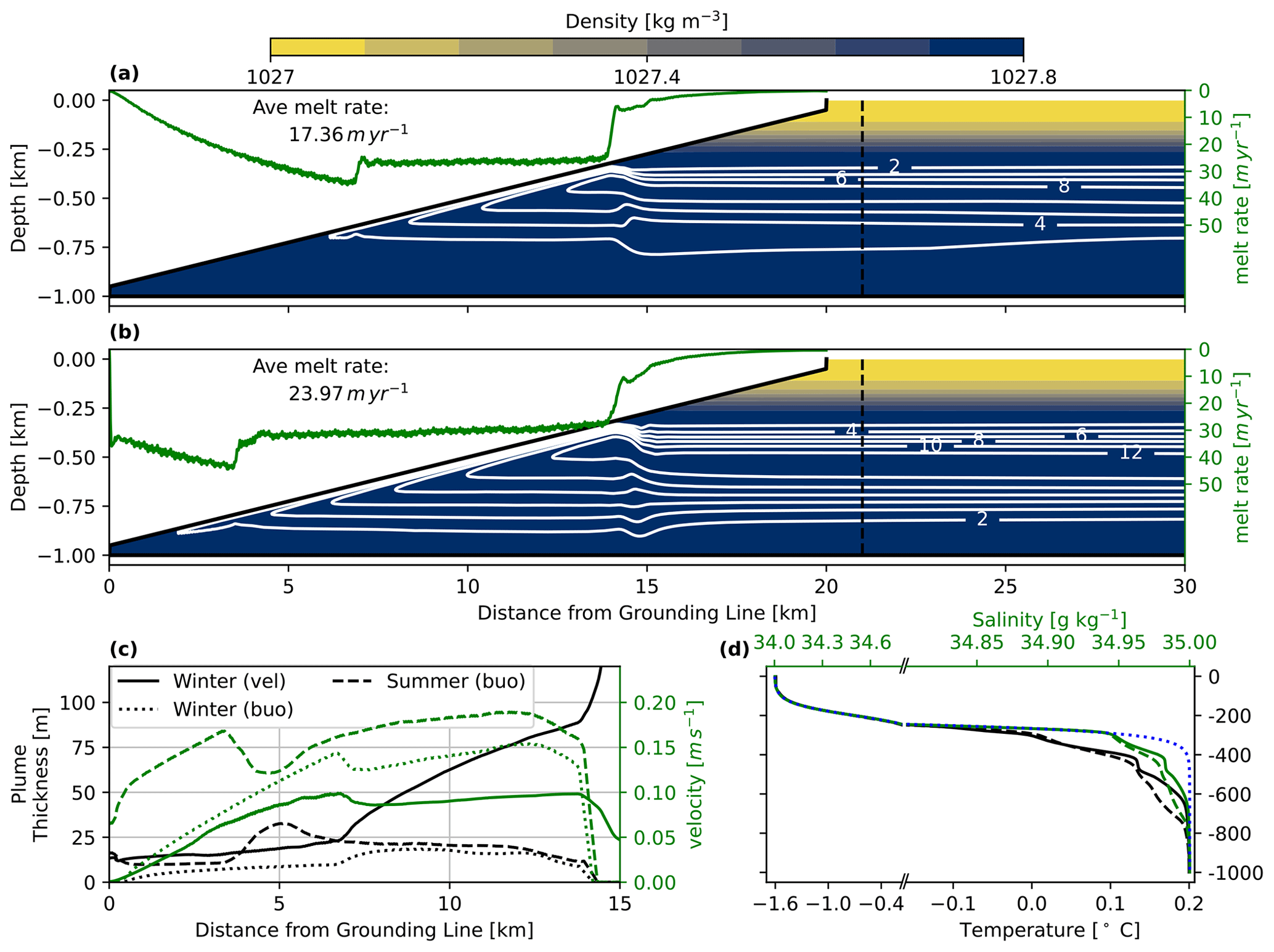
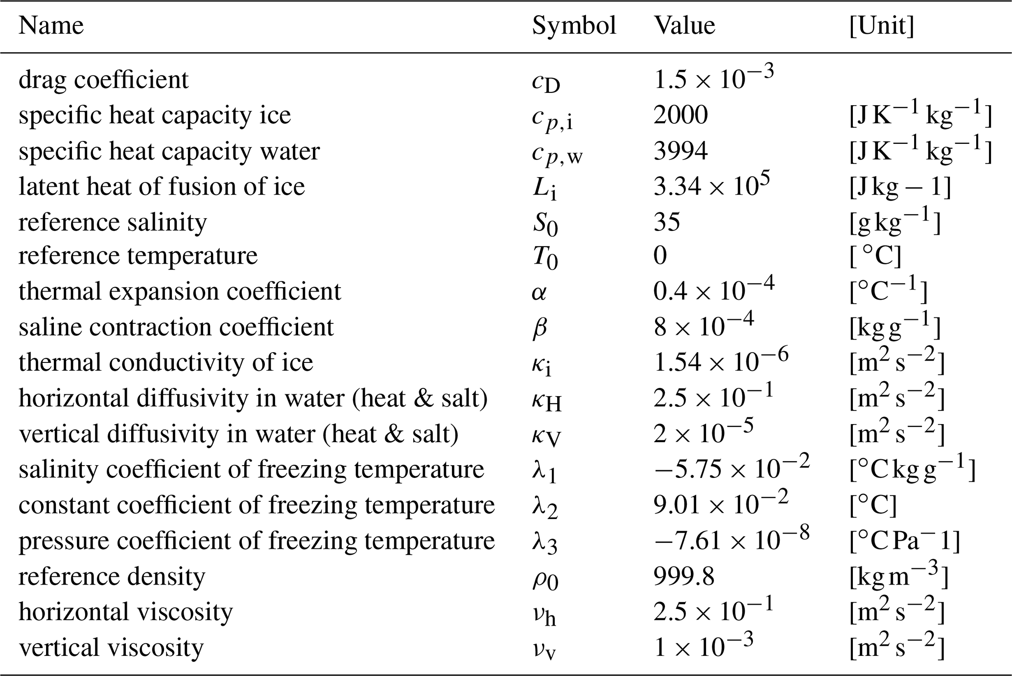
Figure 1 (a) The stream function (white contours in m² s⁻¹) of the steady circulation superimposed on the density (σ, colours) and the melt rate (green line, right axis) along the ice–ocean interface (black line) for control_win. The black dashed line indicates the location of profiles shown in Figs. 3 and 7; (b) same as in (a) but for control_sum; (c) the plume thickness (black) calculated based on a combined velocity and buoyancy criterion (“buo”) for summer (dashed) and winter (dotted) control simulation and for winter based on only velocity (“vel”, solid); and the vertically averaged plume velocity (green). (d) Initial and open-ocean boundary condition profiles of salinity and temperature (showing as one blue dotted line for the chosen axes limits) and the steady-state temperature (black) and salinity (green) profiles of the summer (dashed) and winter (solid) control simulations at x = 21 km.

The domain's dimensions and geometry are shown in Fig. 1a and b. We focus on the circulation in the ice shelf cavity, i.e. the first 30 km of the SOF with a horizontal grid spacing of dx= 10 m along the fjord axis. The model width in the across-fjord direction is one grid cell of size dy= 10 m. The domain is 1000 m deep divided in 300 equally spaced vertical levels (dz= 3.33 m). The first 20 km of the domain is covered by a floating ice shelf representing the RG's ice tongue. The ice tongue terminates in a 50 m deep front at x= 20 km. To represent the observations, the ice base is set to be a constant linear slope of s=0.045, which is equivalent to an angle of ϕ = 0.04^∘, connecting the grounding line and the lowest point of the calving front (Fig. 1a). In the absence of detailed data about the ice and sea floor topography at the grounding line, we chose to keep a vertical wall below the lowest point of the ice shelf of 50 m including a 20 m vertical SGD region (970 to 950 m; see Sect. 2.2) to leave room for inflowing AW and to avoid generation of strong property gradients at the corner of the domain. The bottom of the domain is flat. A quadratic drag is applied at the bottom of the domain and the ice.

All experiments are started from rest, initialized with horizontally uniform salinity (S) and temperature (T) profiles. In the control simulations these approximate the hydrographic profiles taken glacier ward of the inner sill just in front of the ice front (Station 16, 17 from Fig. 1 in Jakobsson et al., 2020). For simplicity and because the nonlinear effects are small in the range of S–T values, we are considering a linear equation of state (EOS) for the density ρ:

$$\begin{array}{}\text{(1)}& \mathit{\rho }={\mathit{\rho }}_{\mathrm{0}}[\mathrm{1}-\mathit{\alpha }(T-T_{\mathrm{0}})+\mathit{\beta }(S-S_{\mathrm{0}}\left)\right],\end{array}$$

with parameters listed in Table 1. Subgrid-scale processes are parameterized using a Laplacian eddy diffusion of temperature, salinity and momentum with constant coefficients as in the MITgcm fjord simulation of comparable resolution by Sciascia et al. (2013). In the horizontal dimension we apply equal values of diffusion coefficients for temperature, salinity and momentum (horizontal Prandtl number of unity), while in the vertical the viscosity is higher than tracer diffusivity to ensure numerical stability (Table 1). The MITgcm applies the semi-implicit pressure method for nonhydrostatic equations with a rigid-lid, variables co-located in time and with Adams–Bashforth time stepping. The advective operator for momentum is second-order accurate in space. We apply a third-order direct space–time tracer advection scheme with flux limiter due to Sweby (https://mitgcm.readthedocs.io/en/latest/index.html, last access: 4 July 2023; Sect. 2.17).

The northern border of the fjord (at x = 32 km) is the only open boundary. The outflow is balanced at the boundary yielding a net-zero cross-boundary flow. Temperature and salinity are restored to the initial conditions in a 2 km wide restoring zone with a restoring timescale of 1 d at the innermost grid point (x = 30 km) and 1 h at the outermost point (x = 32 km). An experiment conducted in a horizontally extended domain (not shown here) shows that the boundary is sufficiently far away from the ice to have negligible effects on the evolution of the circulation underneath the ice tongue. We set up a winter control simulation (control_win) without any SGD and a summer control simulation with SGD (control_sum; see Sect. 2.2).

2.1 Basal melt parameterization

To parameterize the basal melt processes at the RG's ice shelf, we use the SHELFICE package¹ (Losch, 2008) applying ice–ocean interactions in an interface mixed layer, defined as the uppermost grid cell adjacent to the ice–ocean interface (Dansereau et al., 2013; Cai et al., 2017; Jordan et al., 2018). Freezing and melting processes occur at the infinitesimal boundary layer at the interface and are parameterized employing the three-equation formulation (Hellmer and Olbers, 1989; Holland and Jenkins, 1999):

$$\begin{array}{}\text{(2)}& {\displaystyle }{T}_{\mathrm{b}}={\mathit{\lambda }}_{\mathrm{1}}{S}_{\mathrm{b}}+{\mathit{\lambda }}_{\mathrm{2}}+{\mathit{\lambda }}_{\mathrm{3}}{P}_{\mathrm{b}}\text{(3)}& {\displaystyle }{c}_{p,\mathrm{w}}{\mathit{\rho }}_{\mathrm{i}}{\mathit{\gamma }}_{\mathrm{T}}(T_{\mathrm{w}}-T_{\mathrm{b}})=-L_{\mathrm{i}}q-{\mathit{\rho }}_{\mathrm{i}}{c}_{p,\mathrm{i}}{\mathit{\kappa }}_{\mathrm{i}}{\displaystyle \frac{(T_{\mathrm{s}}-T_{\mathrm{b}})}{H_{\mathrm{i}}}}\text{(4)}& {\displaystyle }{\mathit{\rho }}_{\mathrm{i}}{\mathit{\gamma }}_{\mathrm{S}}(S_{\mathrm{w}}-S_{\mathrm{b}})=-S_{\mathrm{b}}q.\end{array}$$

The interface boundary layer temperature (T_b) is the in situ freezing point temperature obtained from the boundary layer pressure and salinity (P_b and S_b, respectively) using the linear EOS (Eq. 1) where λ_j are constants. Equations (3) and (4), which describe heat and salt balances at the interface, respectively, are used to calculate S_b and q, where q is the upward freshwater flux (negative melt rate, in units of freshwater mass per time), and L_i is the latent heat of fusion. Upward heat flux implies basal melting (a downward freshwater flux), hence the minus sign (Losch, 2008). As in Cai et al. (2017) we assume a linear temperature profile in the ice and approximating the vertical temperature gradient in the ice as the difference between the ice surface (T_S = −20 ^∘C) and interface (ice bottom) temperatures (T_b) divided by the local ice thickness. Subscript w refers to the properties in the interface mixed layer. The values of parameters are listed in Table 1.

Exchange coefficients for salt (γ_S) and heat (γ_T) are calculated online (Holland and Jenkins, 1999) based on the along-ice boundary layer velocity $u^{\ast }=c_{\mathrm{D}}\sqrt{u_{\text{BL}}^{\mathrm{2}}+w_{\text{BL}}^{\mathrm{2}}}$, where c_D is the model drag coefficient and u_BL and w_BL are the local horizontal and vertical boundary layer averaged velocities. This yields the following:

$$\begin{array}{}\text{(5)}& {\mathit{\gamma }}_{\text{T,S}}={\displaystyle \frac{u^{\ast }}{{\mathrm{\Gamma }}_{\text{Turb}}+{\mathrm{\Gamma }}_{\text{Mole}}^{\text{T,S}}}},\end{array}$$

where Γ_Turb and ${\mathrm{\Gamma }}_{\text{Mole}}^{\text{T,S}}$ are the turbulent and molecular exchange parameters defined as in Holland and Jenkins (1999) Eqs. (15) and (16). The linear dependency of the exchange coefficient on the along-ice velocity u^∗ is expected to lead to a super-linear dependency of melt on the thermal forcing, because u^∗ is approximated to increase with increasing thermal forcing through the change in buoyancy from enhanced melting (e.g. Jenkins, 1991; Holland et al., 2008b; Jenkins, 2011; Lazeroms et al., 2018).

Equations (2)–(4) are solved for boundary temperature and salinity and the melt rate q at every time step. The freshwater mass flux output (in $\mathrm{kg}{\mathrm{m}}^{-\mathrm{2}}{\mathrm{s}}^{-\mathrm{1}}$) is negative for melting, i.e. a downward mass input into the ocean. The temperature and salinity changes due to fresh water flux are implemented using virtual fluxes in the respective tendency equations. As the model employs partially filled cells, the parametrization uses a simple boundary layer averaging over vertical grid size dz. Velocities are averaged onto the tracer grid points. For further details about the ice shelf parametrization the interested reader is referred to Losch (2008).

2.2 Sensitivity experiments

We set up two sets of experiments: one without SGD and one with varying SGD. The goal of the first set of experiments is to elucidate on the dependency of basal melt on the oceanic thermal forcing. The second set is supposed to shed more light on how different SGD volumes influence the basal melt. Selected experiments are listed in Table 2. For a complete list of experiments the interested reader is referred to the Appendix Tables A1 and A2.

Figure 2 Initial and open-ocean temperature profiles for a selected set of experiments with varying AW temperature.

Oceanic thermal forcing

First, we investigate a scenario of warming AW temperatures. To this end, we conduct a set of experiments with varying AW temperature (T_AW) while keeping PW temperature in the surface layer constant, applied as initial condition and boundary condition at the open-ocean boundary. The temperature profiles used to initialize and force the model are shown for a selected set of experiments (including warmest and coldest) in Fig. 2. A full list of experiments with their respective AW temperature is given in Table A1. The salinity profile is the same for all experiments.

To quantify the response of the system in terms of melt rate and circulation changes to changing oceanic thermal forcing (by varying T_AW), we define an average temperature forcing $\mathrm{TF}=T_{\text{GL}}(x_{\text{GL}},z_{\text{GL}})-T_{\mathrm{f}}(x_{\text{GL}},z_{\text{GL}}$) for each experiment, based on the time-averaged fields when the model is in a statistical steady state (model days 61–100). T_GL is the time-averaged water temperature at the grounding line (x_GL,z_GL), and T_f is the freezing point temperature evaluated at the same point using the local water salinity S(x_GL,z_GL). Note that the water at the grounding line is a slightly modified AW, so T_GL is close to T_AW. Furthermore, T_f at the grounding line is essentially constant throughout all experiments at T_f = −2.68 ^∘C; hence we can approximate $\mathrm{TF}\approx T_{\text{GL}}+\mathrm{2.68}{}^{\circ }\mathrm{C}$ (see Tables 2, A1 and A2). We apply a wide range of AW temperatures to quantify the response of the melt rate and the resulting circulation to varying TF with more confidence.

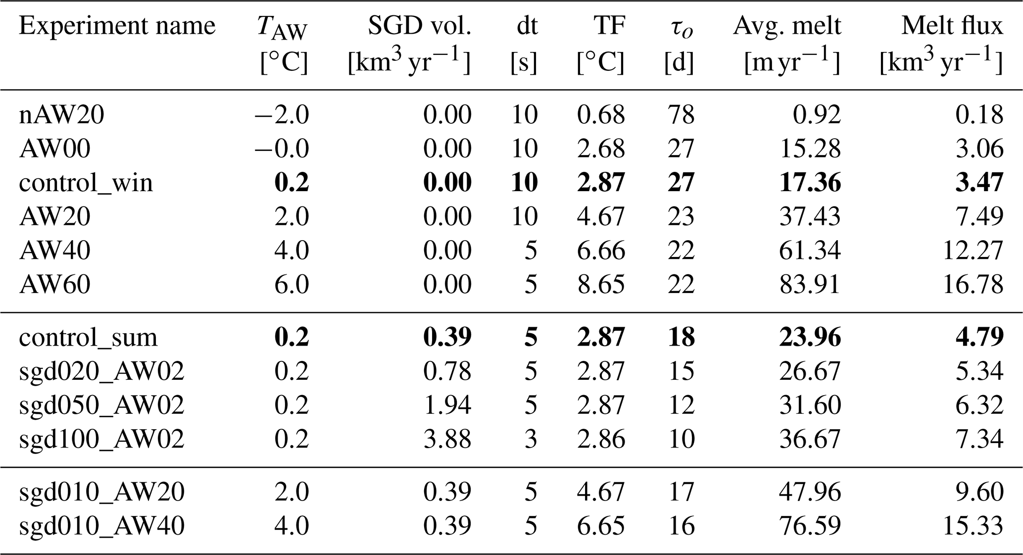
Table 2 Setup parameters and diagnostics for selected experiments. From left to right, AW temperature, subglacial discharge volume in percent of control_win integrated melt volume, model time step, TF, overturning timescale, averaged melt rate and integrated melt flux for a 10 km wide fjord. For a complete account of all experiments see Appendix A. Values from the winter and summer control simulations are highlighted in bold.

Subglacial discharge

A second set of sensitivity experiments is conducted to investigate the influence of SGD. In lieu of lacking information about the RG's subglacial channel geometry, we assume that the subglacial flux is dispensed evenly across the grounding line in a series of ice cavities 10 m (domain across-fjord width dy) in width and 20 m in height, analogous as in 2D setups of Sciascia et al. (2013) and Cai et al. (2017). The SGD volume fluxes are set in relation to the integrated melt flux of the winter control simulation. Direct observations at a nearby glacier (79NG) found that about 11 % of the total fresh water leaving the cavity was from subglacial discharge (Schaffer et al., 2020). Therefore we set our lowest SGD volume (SGD010) to around 10 % of total melt from control_win. Higher SGD is applied in multiples of SGD010. Using regional climate models, Mankoff et al. (2020) and Slater et al. (2022) report estimated SGD of 357 m³ s⁻¹ = 11.26 km³ yr⁻¹ for a fjord width of around 11 km. Our highest SGD value, assuming a 10 km wide fjord, is around 40 % of their value. For exact values of SGD volume applied in the presented simulations, please refer to Tables 2 and A2.

The subglacial flux is implemented as a source term in tracer and momentum conservation equations using MITgcm source and relaxation package RBCS (https://mitgcm.readthedocs.io/en/latest/phys_pkgs/rbcs.html, last access: 4 July 2023). The discharge velocity is calculated as the ratio of the SGD volume flux to the area of the model cells where the SGD is applied. Note that the discharge velocity in MITgcm is applied in horizontal direction. The SGD fluxes for various experiments are presented in Table A2. These are rescaled from the dy = 10 m wide model domain to the estimated RG grounding line width of 10 km. We use a conservative third-order direct space–time tracer advection scheme with flux limiter (Sect. 2) to avoid tracer extremes and the possibility of salinity going negative during the numerical integration when implementing SGD.

Steady state

All simulations were run for 100 d with a time step of 2–10 s depending on the strength of the oceanic thermal and/or SGD forcing to achieve model stability (Table 2). The statistically stationary equilibrium is reached after ca. 40 d for volume-averaged kinetic energy, circulation timescales and melt rates for all the runs (Figs. B1 and B2), which is in line with an overturning timescale of 20–30 d. The integrated temperature change does not stabilize completely (Fig. B1) for the two warmest runs, but the deviations do not have a significant effect on the other properties. For further analysis we use the last 40 d of simulation (model days 61–100). The experiment setup details and key diagnostic values for a selected subset of experiments are given in Table 2. For the complete list of experiments we refer the reader to Sect. A.

3 Results

3.1 Winter and summer control simulations

The steady-state (model days 61–100) melt rates and circulation under the RG ice tongue for control_win and control_sum simulations are shown in Fig. 1a and b, respectively. Both cases exhibit an estuarine circulation typical of glacial fjords (Straneo and Cenedese, 2015): the warm AW inflow in the lower layer supplies heat to the ice base forcing basal melting. The meltwater input drives a buoyant plume, which rises into the base of the pycnocline (located at about 400 m depth) where it reaches its level of neutral buoyancy and forms a horizontal outflow jet towards the open boundary. The overturning time is estimated from the model domain volume (V_d) divided by the integrated AW volume transport at x = 21 km (${\mathit{\tau }}_{\mathrm{o}}=\frac{V_{\mathrm{d}}}{\int \int u_{\text{AW}}\left(z\right)\mathrm{d}z\mathrm{d}y}$) and yields 27 d (winter) and 18 d (summer, Table 2).

Restoring to the initial stratification at the open boundary results in a continuous oceanic heat transport toward the ice base sustaining the basal melt (Eqs. 2–4). The steady-state melt rates along the ice base are shown in Fig. 1a and b, and the average values are shown in Table 2. Both winter and summer control simulations exhibit positive average melt rates, corresponding to equivalent ice thickness loss and potential glacier retreat. In control_win, the average melt rate is 17.36 m yr⁻¹, but the melt rates are variable along the ice base (Fig. 1a and b): rising from zero at the GL to a maximum of 35.08 m yr⁻¹ at about 7 km where they drop slightly to a value around 27 m yr⁻¹ persisting until 14 km and then dropping towards zero. This spatial melt rate distribution is related to the buoyant plume properties (see below). The meltwater flux integrated along the 20 km long ice shelf amounts to 3.47 × 10⁵ m² yr⁻¹ per unit width or 2.95–3.47 km³ yr⁻¹ for the estimated glacier tongue width of 8.5–10 km. For the control summer simulation, the average basal melt increases to 23.96 m yr⁻¹ (or 4.07–4.79 km³ yr⁻¹), which is an increase of 38 % compared to the winter control. The summer control shows a similar variability of melt rates along the ice base to the winter control but for the immediate buoyancy input at the GL, which leads to the melt rate maximum shifting the transition zone from 7 km to closer to the GL at 4 km where the maximum melt rate is 44.50 m yr⁻¹, and a subsequent drop to an approximately constant 30 m yr⁻¹ persisting until 14 km and then dropping towards zero. This shift of transition zone (7 km in winter vs. 4 km in summer) collocates with a downward thickening of the ambient pycnocline (Fig. 1d).

We will here describe the melt-driven circulation for the winter simulation and examine effects of changes of thermal forcing and SGD in the following sections. To characterize the buoyant plume, we define the plume as the region beneath the ice base where u>0 (the flow is towards the open ocean). We tried alternative definitions of the plume based on the temperature and salinity difference compared to the ambient and prescribed stratification. These resulted in a narrower or wider plume over the distance between 7 and 14 km depending on the value of temperature and salinity used. For values closer to these of ambient stratification, the resulting plume was wider. As the difference encompasses the region of no horizontal flow outside the plume (by definition u≤0 here), this has no impact on the further calculations of, for example, plume transport. Using a buoyancy criterion (i.e. temperature and salinity combined) and defining a threshold (75th percentile) results in a narrower and relatively well mixed plume, i.e. in characteristics more comparable to the plume of Jenkins (1991, 2011). To quantify this, we show the plume thickness and averaged plume velocity ($u_{\mathrm{p}}=\sqrt{u^{\mathrm{2}}+w^{\mathrm{2}}}$) in Fig. 1c. Clearly distinguishable are two different plume regimes during its ascent along the ice base, no matter the way of defining the plume: the accelerating plume and the thickening plume. When using the velocity criterion, in the accelerating plume regime close to the GL, the plume has a thickness of around 20 m, while the vertically averaged plume velocity increases steadily to a maximum of 0.1 m s⁻¹ at 7 km. In the thickening regime the velocity is around 0.095 m s⁻¹ and the plume thickness increases from 20 to 90 m between 7 and 14 km. The depth of the transition from accelerating to thickening plume is linked to the ambient stratification in the fjord (Fig. 1d; see Sect. 3.2 and 3.3). The average plume thickness is around 40 m for all experiments.

Note however that the plume defined by velocity only is still stratified, so it is not fully equivalent to the “well-mixed plume” in the sense of the plume model of Jenkins (2011). If we define the plume by adding a buoyancy criterion (only the 75th percentile of buoyancy values in the velocity plume), the plume is narrower with higher average velocities compared to the original definition based on velocity only (Fig. 1c). Notably, the plume accelerates strongly in the first regime to a local maximum average velocity of 0.14 m s⁻¹ and shows a significant decrease of velocity at the regime transition but subsequently starts again to accelerate in the second regime. The overall higher velocities using the buoyancy plume definition arise because the region of low velocities further away from the ice is not considered.

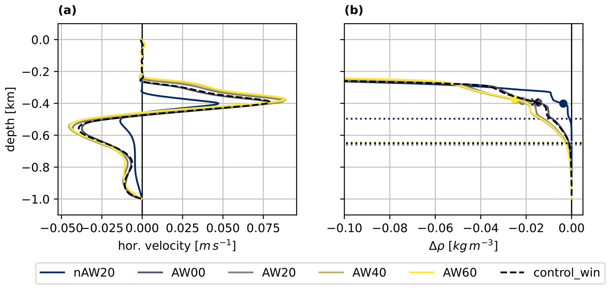
Figure 3 Profiles (solid lines) at 21 km from the control_win and selected oceanic thermal forcing experiments of (a) horizontal velocity and (b) density change with respect to bottom density, $\mathrm{\Delta }\mathit{\rho }=\mathit{\rho }\left(z\right)-\mathit{\rho }(z=\mathrm{1}\mathrm{km})$. Dots in (b) indicate the depth of maximum horizontal velocity. The dotted horizontal lines in (b) indicate the depth of maximum melt (corresponding to the plume's regime transition point depth).

At 14 km, the plume velocity drops towards zero (Fig. 1c) which marks the location where the plume separates from the ice (Fig. 1a and b) and forms a horizontal outflow jet towards the open boundary. The outflow layer is about 250 m thick (spanning 250–500 m depth) with a maximum velocity at 400 m (Fig. 3a). The outflow forms a T–S transition layer between the AW and the PW, which was smoothed out in the idealized initial profiles (Figs. 1d and 3b). This layer is characterized by a cooling and freshening compared to the initial profile, in line with what would be expected from glacially modified water. This glacially modified layer can also be found in the observations of (Jakobsson et al., 2020) (see their Fig. 2), lending confidence to the model results. The outflow at intermediate depth is balanced by an AW inflow in the bottom layer with a maximum velocity of −0.04 m s⁻¹ just below 500 m and a secondary maximum close to the bottom (Fig. 3a). The plume is not sufficiently buoyant to penetrate into the upper layer of PW, which remains undisturbed.

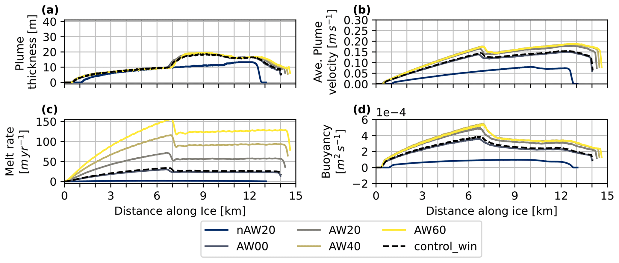
Figure 4 Plume properties for simulations with varying oceanic thermal forcing (AW temperatures) as a function of distance from the grounding line along the ice: (a) plume thickness, (b) averaged plume velocity, (c) melt rate and (c) buoyancy (see text).

3.2 Sensitivity to oceanic thermal forcing

We will first describe the results of the winter simulation without SGD for different temperature scenarios, before looking into the effect of the varying SGD (Sect. 3.3). We applied a wide range of AW temperatures to quantify the response of the melt rate and the resulting circulation to varying oceanic thermal forcing with more confidence, which is shown in Figs. 3 and 4. The structure of the circulation and the distribution of the plume properties is the same for all experiments, except of those with very low AW temperatures (TF < 2 ^∘C, T_AW < −1.0 ^∘C). The plume thickness and its velocity (Fig. 4a and b), thus the volume transport, change only slightly in response to the increased melt for warmer experiments (Fig. 4c). The increased meltwater input freshens and cools the plume and the outflow, sharpening the density gradient at the base of the pycnocline in the outflow without changing its thickness (Fig. 3b). Figure 4d shows the buoyancy in the plume, estimated from the density difference between the local plume density (ρ_p) and the ambient ocean density (ρ_a) at 21 km: $b=\frac{{\mathit{\rho }}_{\mathrm{a}}(x=\mathrm{21}\mathrm{km},z)-{\mathit{\rho }}_{\mathrm{p}}(x,z)}{{\mathit{\rho }}_{\mathrm{0}}}g$. Because of the competing effect of freshening and cooling on the density, there is no effective change of buoyancy forcing with increasing TF. For the coldest experiments, i.e. weak oceanic thermal forcing, the melt rate is lower and the plume shows the shift to the secondary regime only around 10 km (Fig. 4a and b) at a depth of around 500 m (Fig. 3b).

The horizontal dashed lines in Fig. 3b show the depth of maximum decrease of vertically averaged plume velocity before the detachment, which is also the depth at which the plume transitions from the accelerating to the thickening regime (Sect. 3.1). For all experiments the depth of the transition coincides with the base of the pycnocline marked by Δρ < 0 (at about 620 m depth). This suggests that the spatial structure in the melt rates and the transition between the accelerating and thickening plume at 7 km is determined by the ambient stratification. The evolution of the vertically averaged plume buoyancy along the ice underpins this conclusion further, as the maximum buoyancy coincides with the point of regime transition for various TF experiments (Fig. 4d).

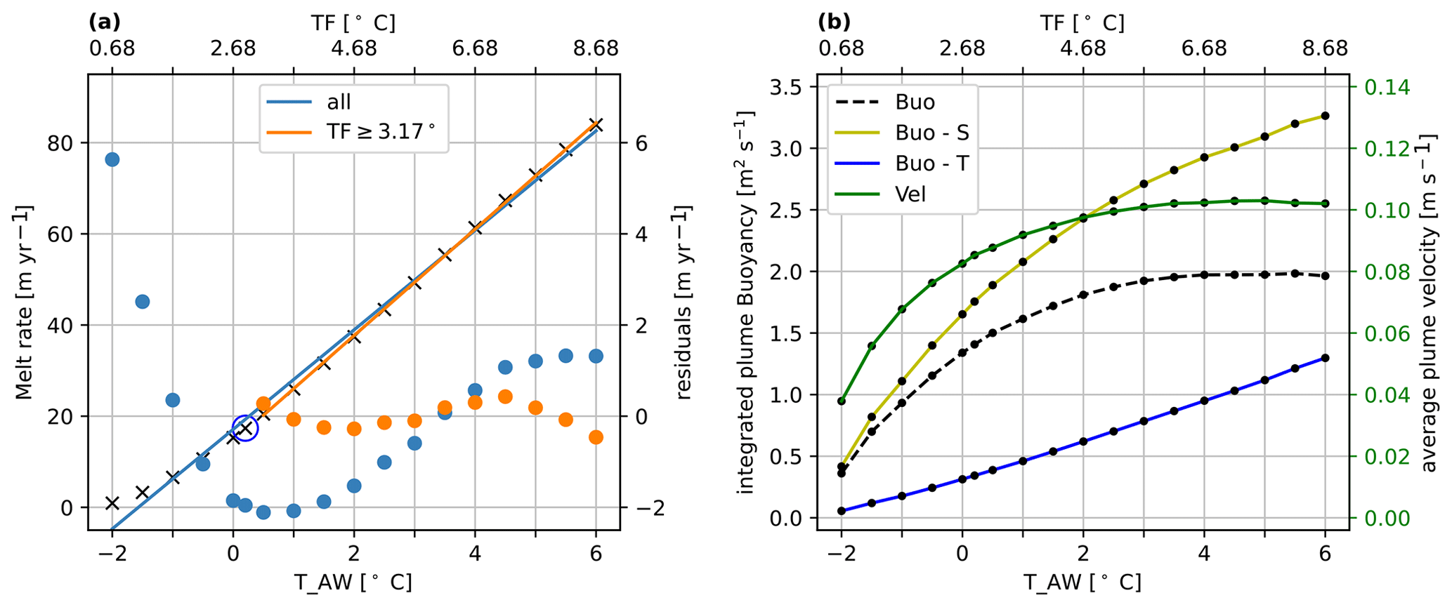
Figure 5 (a) The average melt (left ordinate axis) as a function of AW temperatures (T_AW; bottom abscissa) corresponding to temperature forcing (TF; top abscissa) for winter experiments (without subglacial discharge). Superimposed are the linear fits for all experiments (blue line) and for intermediate to warm experiments only (orange line; see text). The corresponding residuals (right ordinate axis) are plotted with dots. control_win is marked with a blue circle. (b) The plume-averaged buoyancy due to temperature (Buo-T; blue; absolute values of the negative function are shown), salinity (Buo-S; yellow) and the combined influence on density (Buo, black dashed).

Figure 5a shows the average melt rate for a wide range of TF. We quantify the response to oceanic thermal forcing using regression analysis (e.g. Storch and Zwiers, 1984) and a resampling technique. A linear regression fit has high residuals for low TF values. We then construct sample subsets by successively excluding data points from cold experiments, starting with the coldest, and re-evaluate the linear fit. In doing so, we find the highest coefficient of determination (R²) and the lowest root mean squared error of a linear fit for experiments with a temperature forcing TF ≥ 3.18 ^∘C (AW05, Fig. 5). The adjusted linear fit has smaller residuals for all TF ≥ 3.18 ^∘C (Fig. 5a) implying a non-linear dependency of melt flux on TF for TF ≤ 2.88 ^∘C (control_win) and a linear dependency for TF ≥ 3.18 ^∘C (AW05). The fitted linear increase of melt per degree warming of AW is 11.69 m yr⁻¹ K⁻¹ or roughly two-thirds of the modelled melt under winter conditions (17.36 m yr⁻¹) per degree warming.

The integrated cooling and freshening effect on the plume's buoyancy is summarized for all temperature sensitivity experiments in Fig. 5b. The buoyancy due to the plume temperature (Buo-T) and salinity (Buo-S) is calculated as the buoyancy in Fig. 4 but from the respective difference between temperature and salinity using the linear EOS (Eq. 1) and integrated vertically and horizontally over the plume. For higher temperature forcing (TF ≥ TF_c = 3.18 ^∘C, Table A1) the buoyancy is no longer increasing linearly with TF. The effect of temperature and salinity start to balance one another and the total buoyancy becomes independent of temperature for experiments with temperature forcing of TF > 6.18 ^∘C (AW35), resulting in a plateauing of average plume velocities (green in Fig. 5b). We elaborate on this in Sect. 4, “Response to oceanic thermal forcing”. This explains the very weak response of plume velocity to the oceanic thermal forcing at higher TF (Fig. 4b). Consistently, the fjord overturning timescale decreases with TF for colder experiments (implying a faster overturning) but saturates around 22–23 d for the warmer simulations (Tables 2 and A1).

Figure 6 Same as Fig. 4 but for different SGD volume fluxes and AW temperatures.

3.3 Sensitivity to subglacial discharge

SGD has a pronounced effect on the basal melt rates. The average melt rate for the control_sum simulations (where SGD is set to 10 % of the average basal melt flux for the control winter; Table 2) is increased by 38 % (from 17.36 to 23.96 m yr⁻¹, Table 2). For the experiment with the highest SGD (sgd100_AW02 in Table 2) the increase in melt is 111 % (36.67 m yr⁻¹).

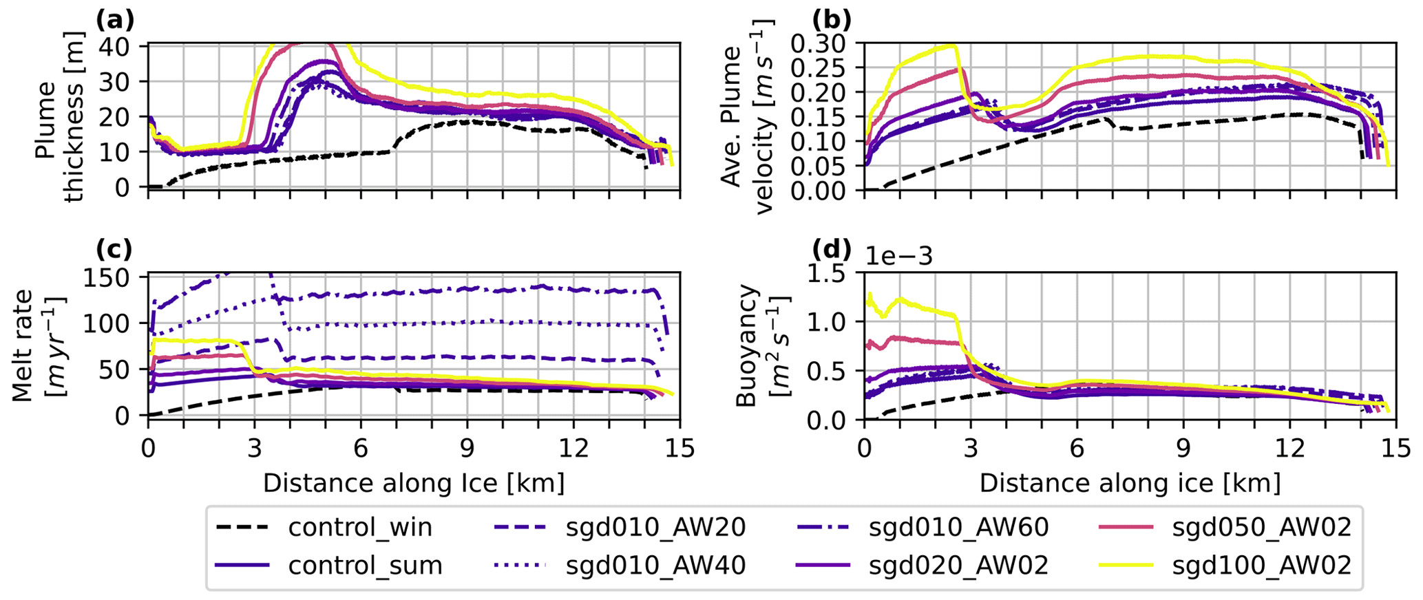
Not only does the total melt change, but so does the melt rate distribution along the ice base and the plume properties (Fig. 6). The buoyancy input from SGD leads to high plume velocities at the GL resulting in higher melt rates there (Fig. 6b and c). While for all experiments the accelerating and thickening plume regime identified in control_win are distinguishable by thickness, velocity and melt (Fig. 6a–c), the point of transition moves towards the GL. For control_sum the transition point jumps more than 3 km closer to the GL (from 7 km in control_win to 3.5–4 km in control_sum). When increasing the discharge further, the migration of the point of transition towards the GL becomes less rapid (to 3–3.5 km for 20 % discharge, to < 3 km for 50 % and 100 % discharge). This does not immediately reflect in a thickening of the plume (Fig. 6a), which is only slightly increased compared to the control_sum. Despite starting with already high velocities, the plume does accelerate further in the first regime, while the melt rate increases and the thickness stays constant, similar to the winter simulations. In the thickening regime, after a slow down of the plume, the velocities and melt rates become almost constant (Fig. 6).

Figure 7 As Fig. 3 but for different SGD volume fluxes.

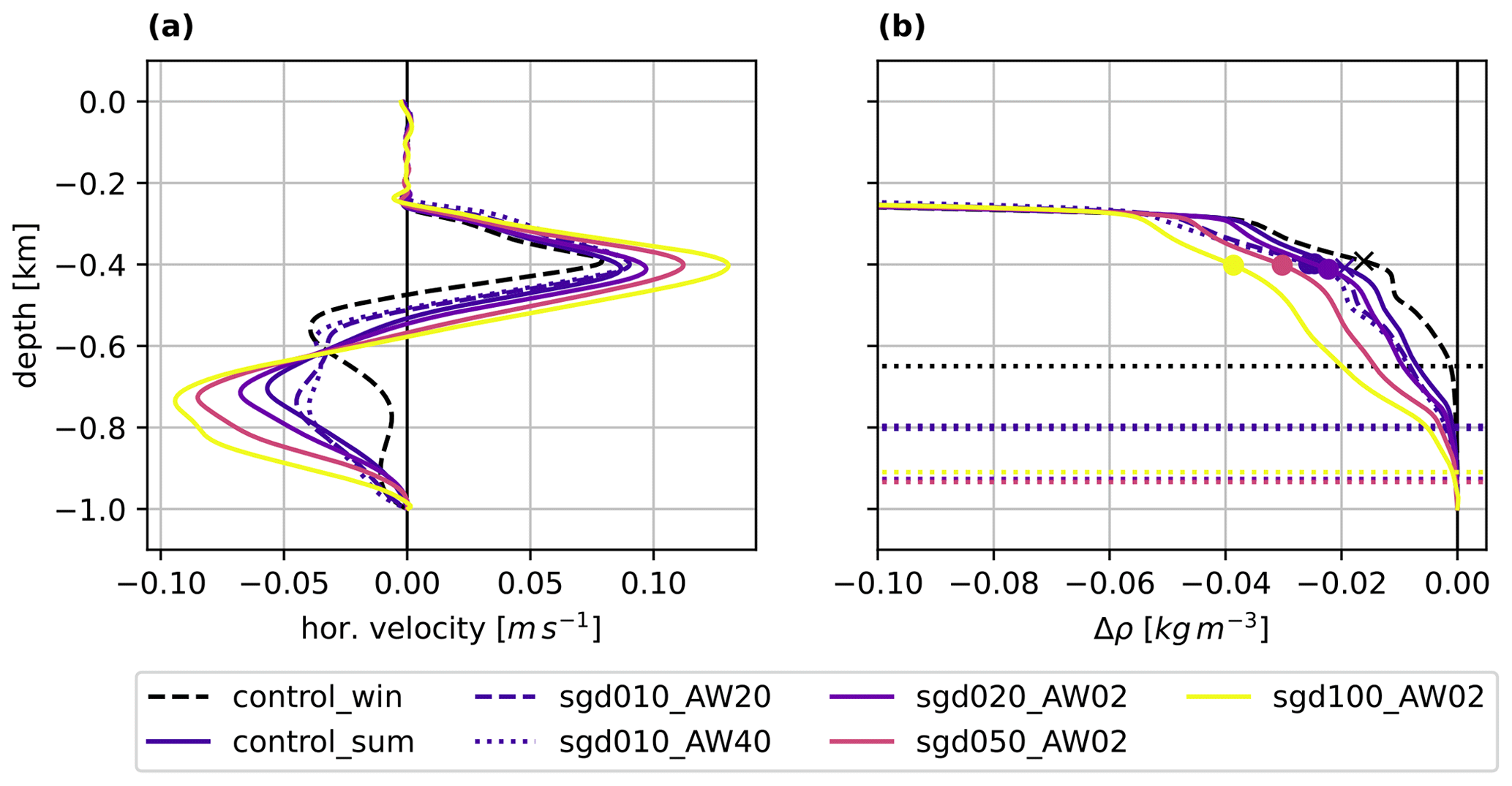
The increased meltwater input in simulations with SGD leads to a fresher, colder and faster outflow and a downward shift of the base of the pycnocline (Fig. 7a and b), more pronounced for experiments with higher SGD. This downward shift of the base of the pycnocline to a depth of about 800 m is related to the spatial structure of the melt rates and the shift of transition zone between the accelerating and thickening plume regimes (Figs. 6a–c and 7b; horizontal dotted lines), consistent with findings in Sect. 3.2 (Fig. 3). The distribution of the plume buoyancy along the ice base underpins this conclusion further, as the sudden decrease in buoyancy coincides with the point of regime transition for all SGD experiments (Fig. 6d).

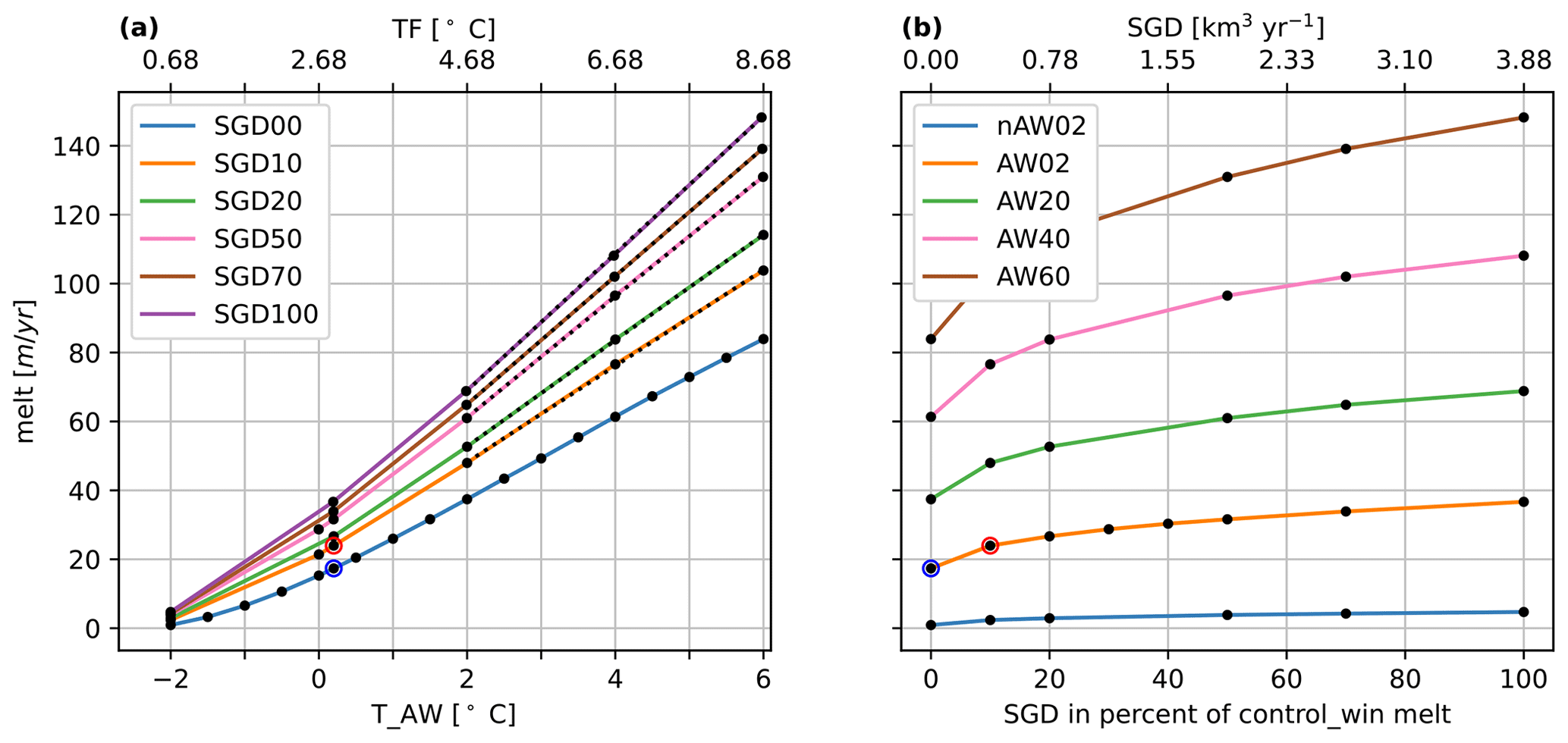
Figure 8 (a) The average melt (left ordinate axis) as a function of AW temperatures (T_AW; bottom abscissa) corresponding to temperature forcing (TF; top abscissa) for summer model experiments with added SGD (dots). The coloured lines link model simulations with equal SGD. Dotted lines, superimposed on the coloured lines, show the linear regression models for the respective SGD experiments. (b) The average melt as a function of SGD (dots). The coloured lines indicate sets of experiments with equal AW temperature. The blue and red circles indicate winter and summer control simulations, respectively.

The effect of oceanic thermal forcing (increasing TF) on simulations with SGD is shown in Fig. 8. It leads to the following observations:

1. The functional response of the melt rate to TF found in the winter simulations (without SGD; Fig. 4a) holds for the simulations with SGD (Fig. 8a). For the experiments conducted, the linear regression (dotted lines in Fig. 7) fit with the simulated melt rates for TF ≥ 3.18 ^∘C.

2. The linear increase of the melt rate becomes stronger, for higher SGD; 14.02 $\mathrm{m}{\mathrm{yr}}^{-\mathrm{1}}{\mathrm{K}}^{-\mathrm{1}}$ for SGD10, 15.47 $\mathrm{m}{\mathrm{yr}}^{-\mathrm{1}}{\mathrm{K}}^{-\mathrm{1}}$ for SGD20, 17.68 $\mathrm{m}{\mathrm{yr}}^{-\mathrm{1}}{\mathrm{K}}^{-\mathrm{1}}$ for SGD50, 18.80 $\mathrm{m}{\mathrm{yr}}^{-\mathrm{1}}{\mathrm{K}}^{-\mathrm{1}}$ for SGD70 and 20.17 $\mathrm{m}{\mathrm{yr}}^{-\mathrm{1}}{\mathrm{K}}^{-\mathrm{1}}$ for SGD100, compared to an increase of 11.71 $\mathrm{m}{\mathrm{yr}}^{-\mathrm{1}}{\mathrm{K}}^{-\mathrm{1}}$ for no SGD. Beware that for SGD experiments the fit is only calculated for the three available data points with TF ≥ 3.18 ^∘C.

3. For experiments with constant TF, the melt rates increase less than linear (in a fractional manner) with SGD (Fig. 8b). The exponents c in the relationship between melt rate M and SGD volume V_sgd, M = $a+b{V}_{\text{sgd}}^c$, are 0.41 for SGD experiments with TF ≈ 0.68 ^∘C (*_nAW20, five experiments), 0.46 for SGD experiments with TF ≈ 2.87 ^∘C (*_AW02, five experiments) and TF ≈ 4.67 ^∘C (*_AW20, five experiments), and 0.47 for SGD experiments with TF ≈ 6.65 ^∘C (*_AW40, five experiments) and TF = 8.67 ^∘C (*_AW60, five experiments). Using the additional experiments available for *_AW02 experiments, the exponent is 0.45 (seven experiments), showing some sensitivity of the fit to the number of data pairs used within a fixed range.

3.4 Comparison with 1D plume model

A comparison between ocean circulation model results and those from the 1D idealized plume model (Jenkins, 1991, 2011) is not straightforward. An ocean circulation model, like MITgcm, includes for example non-linear and viscous terms and resolves the plume with several grid points in the vertical, whereas the 1D model simulates a uniform (in the normal direction to the ice) plume. Nevertheless, we compare the resulting melt rates of both models here, as the plume model is a well-known and established tool to estimate melt rates. In Fig. 9 we compare melt rates from our control_sum simulation with those from the 1D Jenkins plume model. The plume model is set up with the same ice geometry and the steady-state temperature and salinity profile outside the ice shelf cavity at x = 21 km from the MITgcm simulation (control_sum) as the ambient water properties. To investigate the sensitivity to ambient stratification we also run the plume model with uniform ambient properties of AW only. We apply the same SGD flux and channel height (20 m, see Sect. 2) as in control_sum. Entrainment and drag coefficients are taken directly from Jenkins (2011). For a detailed description of the plume model see Jenkins (1991) and Jenkins (2011), and for a detailed description of the setup, please refer to the supplementary material of Jakobsson et al. (2020).

The MITgcm simulation shows around 3 times lower melt rates than the plume model. This can be explained by higher velocities in the plume model (not shown) and could be tuned by changing for example the drag coefficient or the entrainment coefficient (see e.g. Dansereau et al., 2013; Cai et al., 2017; Slater et al., 2022). Since the area-averaged melt rates in our simulations are comparable to those from satellite observations (Wilson et al., 2017; see Sect. 4) we do not attempt any tuning of the MITgcm simulations to the plume model. Importantly, both models show the sensitivity to the stratification (compare “uniform stratification” and “simulated stratification” in Fig. 9), namely a shift in melt rates, which is described in Sect. 3.1 and discussed below (Sect. 4).

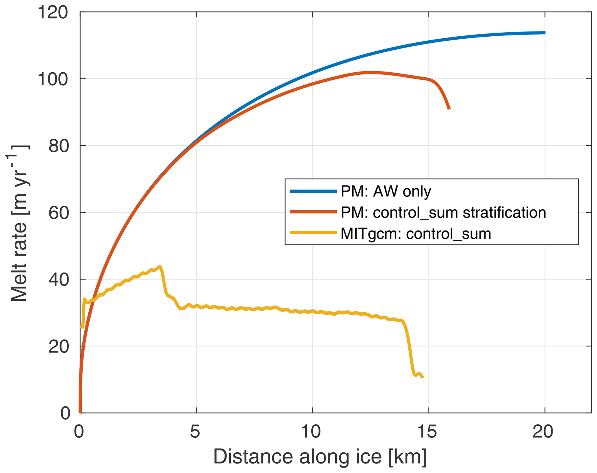
Figure 9 Melt rates from the plume model (“PM”) using a uniform profile with AW temperature and salinity (blue, “AW only”) and the simulated steady-state ambient temperature and salinity profiles from the MITgcm control_sum simulation outside the ice shelf cavity (red, “control_sum stratification”) as ambient water properties. In yellow, the melt rate from MITgcm control_sum simulation.

4 Discussion and conclusions

We used a high-resolution, nonhydrostatic configuration of the MITgcm to investigate basal melt rates and melt-driven circulation in a fjord with an ice tongue. The fjord–ice-tongue geometry is highly idealized, but the grounding-line depth and ice-tongue length are selected to represent RG in SOF, northwestern Greenland. The basal geometry of Ryder's ice tongue varies across the fjord, a feature that cannot be represented in the present two-dimensional model. For simplicity, we have chosen an ice tongue with a linear basal slope, which roughly corresponds to the area-averaged basal slope of Ryder. The control model configuration is based on the observational survey of the Ryder 2019 Expedition and, to our knowledge, our study is the first to investigate aspects of this glacier–fjord system using high-resolution ocean modelling. A protocol of model sensitivity experiments quantified the response to oceanic thermal forcing due to warming Atlantic Water (AW), and to the buoyancy input from the SGD of surface fresh water. We applied broad ranges of varying AW temperatures and SGD fluxes to better resolve the basal melt response to forcing and to make our model experiment more universal and relevant to future development of basal melt parameterizations in climate ice sheet models.

Model representation of the glacier–fjord system

Our control simulations represent salient features of estuarine circulation typical of Greenlandic glacier–fjord systems subject to oceanic thermal forcing due to the AW inflow (Straneo and Cenedese, 2015): the warm AW inflow in the deeper layer supplies heat to the ice base forcing basal melting. The meltwater is fresher than ambient and drives a buoyant plume underneath the ice tongue. The plume rises into the base of the pycnocline where it reaches its level of neutral buoyancy, detaches from the glacier front, and intrudes horizontally into the ambient water forming an outflow jet back towards the open boundary. The entrainment of ambient water in the rising buoyant plume drives a slow flow of ambient waters toward the glacier.

The simulated melt rates for our idealized Ryder ice tongue, which has a linear basal slope, are broadly comparable to the satellite-derived estimates from the real Ryder ice tongue for 2011–2015 by Wilson et al. (2017): our maximum melt rates in the summer control simulation near the grounding line are 40–50 m yr⁻¹, as in the observations, while they are around 20–30 m yr⁻¹ away from the grounding line compared to the observed 10–20 m yr⁻¹. The area-integrated basal melt for the control winter experiment (taking the ice tongue width of 8.5 km) is about 3 km³ yr⁻¹ as compared to the observed 1.8 ± 0.21 km³ yr⁻¹ (Wilson et al., 2017) and about 4 km³ yr⁻¹ for the summer control experiment (Table 2). The simulated steady-state fjord stratification recovers the observed signature of an outflow of glacially modified water, which was smoothed out in the profiles used for initialization, providing additional qualitative support for the feasibility of our model approach (Figs. 1d and 3b).

Spatial structure of basal melt rates and melt-driven circulation

Our high-resolution model simulation allowed us to resolve a spatial pattern of the basal melt and the melt-driven circulation under the ice tongue. In the winter control simulation, the basal melt rates and the plume exhibit a two-regime structure along the ice base (high melt rates in the accelerating plume regime up to 7 km and the lower melt rates in thickening plume regime thereafter up to 14 km). This two-regime structure is insensitive to the way of defining the plume (by buoyancy or velocity). We have diagnosed various plume diagnostics using a velocity criterion, which led to, for example, average plume thicknesses of around 40 m, comparable with what was found in Holland et al. (2008b). Care has to be taken when comparing these diagnostics to the one-dimensional plume model (Jenkins, 2011), where uniform plume properties are assumed. This is not necessarily true in the plume defined using the horizontal velocity. Adding a buoyancy criterion yields a narrower and faster plume (see Sect. 3.1), with almost uniform distribution of buoyancy. The uneven vertical spreading of momentum and tracers (i.e. temperature and salinity) can be attributed to a vertical Prandtl number larger than unity, which leads to a stronger downward diffusion of momentum away from the ice, increasing the region of positive horizontal velocities beyond the region of uniform buoyancy. The increased viscosity is needed in order to obtain stable simulations; increased tracer diffusivity would lead to a smearing out of the thermocline. To our knowledge, small-scale variations in the melt rate have been barely captured by observations (Wilson et al., 2017).

The two-regime structure persists in the sensitivity model runs with varying ocean thermal forcing. Applying an additional buoyancy source in simulations with SGD shifts the transition between the two regimes closer to the grounding line. Our results suggest that this spatial structure of the basal melt rates and the melt-driven circulation is determined by the ambient density stratification as shifts of the transition zone in various sensitivity experiments relate to the downward shifts of the pycnocline and shifts in buoyancy forcing. Notably, in the first regime close to the grounding line, our simulated melt rates in the winter runs (without SGD) show a monotonic increase rather than a broader maximum found in Petermann Glacier simulations of Cai et al. (2017) (their Fig. 2). This monotonic increase is less pronounced in our simulations with SGD (SGD was applied in Cai et al., 2017), but it could also be attributed to different ice geometry (a steep ice base close to the grounding line in their study, which would lead to increased melt rates there). Other factors that could affect the structure of the melt rates, but are unresolved by either modelling study, are the variability of the SGD in the transverse direction as it enters the fjord waters through channels discharging at the base of the glacier's front whose number, sizes, and geometries and time variability are mostly unknown and possibly influenced by the complex networks of drainage channels and crevasses in the glaciers (Chen, 2014) and the presence of basal channels and terraces (Millgate et al., 2013; Dutrieux et al., 2014).

Response to oceanic thermal forcing

In this study, we investigated the response of the melt rates and melt-driven circulation to the oceanic thermal forcing (varying AW temperatures). The form of the applied basal melt parametrization (Eqs. 2 and 3) suggests a non-linear dependence of the basal melt on TF, since the melt rate depends on both the ocean temperature and the plume velocity through the transfer coefficient (Eq. 5). The plume velocity is in turn dependent on TF through the buoyancy input from the melt (Holland et al., 2008b; Jenkins, 1991; Lazeroms et al., 2018). A nonlinear relation was found in former studies of Antarctic ice shelves subject to ocean water temperatures around 0 ^∘C (Holland et al., 2008b). Jenkins (2011) found a transition into a linear response of melt rate on TF for sufficiently high buoyancy input through strong SGD. On the other hand, several modelling studies of vertical tidewater glaciers around Greenland, where ocean temperatures are higher due to the AW inflow, have reported on a linear dependency of melt rates on TF (Xu et al., 2012; Sciascia et al., 2013, 2014). A modelling study of Petermann Glacier, a neighbour of RG, by Cai et al. (2017) found a slightly non-linear dependency of melt on TF using a similar set of sensitivity experiments as presented here and assuming the same relationship for the whole TF range.

Here, we applied a wide range of oceanic thermal forcing (with T_AW up to 6 ^∘C, i.e. higher than typically observed at the Greenland's marine-terminating glaciers; see e.g. Straneo and Cenedese, 2015) and a resampling technique to quantify the response of the melt rate and the resulting circulation to varying TF with a higher statistical confidence. We found that a non-linear relationship holds for the simulations with low TF (TF ≤ 2.88 ^∘C, Fig. 5a), while it becomes linear for higher TF, thus linking up and contextualizing results from the previous studies. Note that using a fully nonlinear EOS instead of the linear approximation (Eq. 1) is unlikely to change our results about the dependency of melt on TF. At the lower ocean temperature range, the difference between a linear and nonlinear EOS is insignificant. At the AW temperatures > 0 ^∘C, the effect of ambient ocean temperature on the plume buoyancy described above is expected to be further enhanced with a nonlinear EOS. A previous study of Sciascia et al. (2013), for example, did use a nonlinear EOS and found a linear dependence of melt on TF for the AW temperatures they considered (0–8 ^∘C), consistent with our result for this range.

We went further in trying to elucidate the aforementioned regime shift in the melt rate response to oceanic thermal forcing by examining the buoyancy forcing of the melt-driven plume. For cold ambient temperatures the plume buoyancy is dominated by the salinity difference between the plume and the ambient water. For increasing TF, i.e. increasing ambient temperature, the following mechanisms are in place. First, the melt rate increases, leading to higher input of fresh and cold meltwater. Second, the cooling due to mixing of the ambient AW becomes more efficient because of the larger temperature gradient between the (warmer) ambient water and meltwater. Hence the cooling close to the ice boundary increases more strongly than the freshening with increasing TF. In Fig. 4b this manifests in the slopes of “Buo-S” and “Buo-T” becoming approximately the same for higher TF. Since salinity and temperature effect are of opposite sign, the net change in buoyancy in the plume with increasing TF diminishes, leading to a flattening of the slope of “Buo”. As a consequence, the plume velocities do not increase further with TF (Fig. 5b), resulting in effectively constant exchange coefficient in Eq. (3) and a linear dependence of melt rates for higher TF. An additional factor could be the dependence of T_b (Eq. 2) and therefore the heat balance (Eq. 3) on S_b. An increased melt rate due to higher TF will decrease salinity at the interface, thereby increasing T_b and decreasing the local temperature difference (T_w−T_b) along the ice. This could potentially be a negative feedback on the melt rate contributing to the observed change in dependency of the melt rate on TF from non-linear to linear at higher TF. These results are generic and relevant for future development of the basal melt parameterizations for marine-terminating glaciers in the climate ice sheet models.

Response to subglacial discharge

SGD, the buoyant freshwater released at depth from under Greenland's marine-terminating glaciers, is sourced largely from atmospheric-driven melting of the ice sheet surface during the summer (Chen, 2014). SGD provides an additional buoyancy source for the plume underneath the ice tongue, leading to higher basal melt rates due to higher plume velocities and entrainment of the ambient warm water (Straneo and Cenedese, 2015). Thus, submarine melting integrates both oceanic and atmospheric influences. A recent study of the relative importance of oceanic and atmospheric drivers of submarine melting at Greenland's marine-terminating glaciers from 1979 to 2018 concluded that in the north, the SGD is at least as important as variability in the oceanic thermal forcing to submarine melt rates, while it exhibits an order of magnitude larger variability on decadal timescales (Slater and Straneo, 2022). Here, we considered the response of the basal melt and melt-driven circulation to varying SGD rates. In lieu of missing accurate observational estimates of SGD, we set it to be a fraction of the total basal melt for the winter control simulation.

We found that the SGD has a pronounced effect on the basal melt rates. The average melt rate for the summer control simulations (where SGD is set to ≈ 10 % of the average basal melt flux for the control winter) is increased by 38 %, and for the experiment with the SGD input set to 100 % of the average winter melt rate the increase in melt is 111 %, consistent with the conclusions of Slater and Straneo (2022) for northern Greenland that there is large seasonal variability in melt rate due to atmospheric forcing through SGD. Given that the SGD values presented here are still lower than the average SGD reported by Slater et al. (2022) for June, July and August, we would expect very high seasonal variability in melt rate at northern Greenland's ice shelves. The additional buoyancy input affects the distribution of the melt rates and plume properties along the ice base, enhancing the melt rate and shifting the transition zone between the plume accelerating and thickening regimes closer to the grounding line. This shift of transition zone collocates with a downward thickening of the pycnocline. The functional response of the melt rate to TF found in the winter simulations (without SGD, see above) holds for the simulations with SGD, but there is stronger linear increase in the melt rate with TF for experiments with SGD as compared to the experiments without SGD. For experiments with constant TF, the melt rates increase less than linearly (in a fractional manner) with the SGD, consistent with the modelling experiments of (Cai et al., 2017) for Petermann Glacier and the theoretical scaling of Jenkins (2011) and Slater et al. (2016). Our values for the exponent vary between 0.4 and 0.5 for the different experiments; they are slightly higher than what is estimated from theory (1/3) and close to those found by Sciascia et al. (2013) (0.33–0.5) and Cai et al. (2017) (0.56).

Future outlook

In this work, we have focused on basal melt rates and melt-driven circulation in the ice cavity under the floating tongue of RG, with restoring to a prescribed ocean stratification at the open boundary 30 km upstream. There are several important aspects considering the model representation of these processes. One is the sensitivity to the model resolution and viscosity and diffusivity. In previous studies using MITgcm in similar applications and resolutions Sciascia et al. (2013) and in particular Xu et al. (2012) found that while the plume got better resolved and the average melt rates increased for higher resolution, the general circulation pattern and results about the dependency on oceanic forcing and SGD were consistent between the different simulations. Similar sensitivities to the vertical resolution and the parametrization of melt processes in different vertical coordinate models are found in other models as well, as shown recently by Gwyther et al. (2020). They conclude that the most realistic representation remains unknown and results always have to be considered with respect to the implementation used.

On the other hand, the melt rate magnitude depends also on other factors, e.g. the friction coefficient (Dansereau et al., 2013), which was used by Cai et al. (2017) to tune the model to the observed melt rates, rather than the model resolution. In our simulation with sloping ice shelf, both vertical and horizontal resolution (and viscosity and diffusivity) need to be taken into consideration in a dedicated sensitivity study. Such a study should consider effects of changing these parameters not only on the basal melt but also on the model representation of the stratification and the mixing between AW and PSW, which in turn influence the ocean heat transport to the ice–ocean interface

Future work will include the influence of sill bathymetry in the 100 km long SOF on the oceanic heat transport to the ice cavity. Other important factors to be considered are the spatial and temporal variability of the SGD (Chen, 2014) and the three-dimensional geometry of the ice base featuring a presence of basal channels and terraces (Millgate et al., 2013; Dutrieux et al., 2014). Including these factors in modelling studies is however contingent upon collecting accurate observational estimates necessary to initialize and evaluate the models.

Appendix A: Overview experiments

Table A1 Setup parameters and characteristic diagnostics for temperature sensitivity experiments. From left to right, Atlantic Water Temperature, subglacial discharge volume in percent of control_win integrated melt volume, model time step, TF, overturning timescale, averaged melt rate and integrated melt for a 10 km wide fjord. Values from the winter and summer control simulations are highlighted in bold.

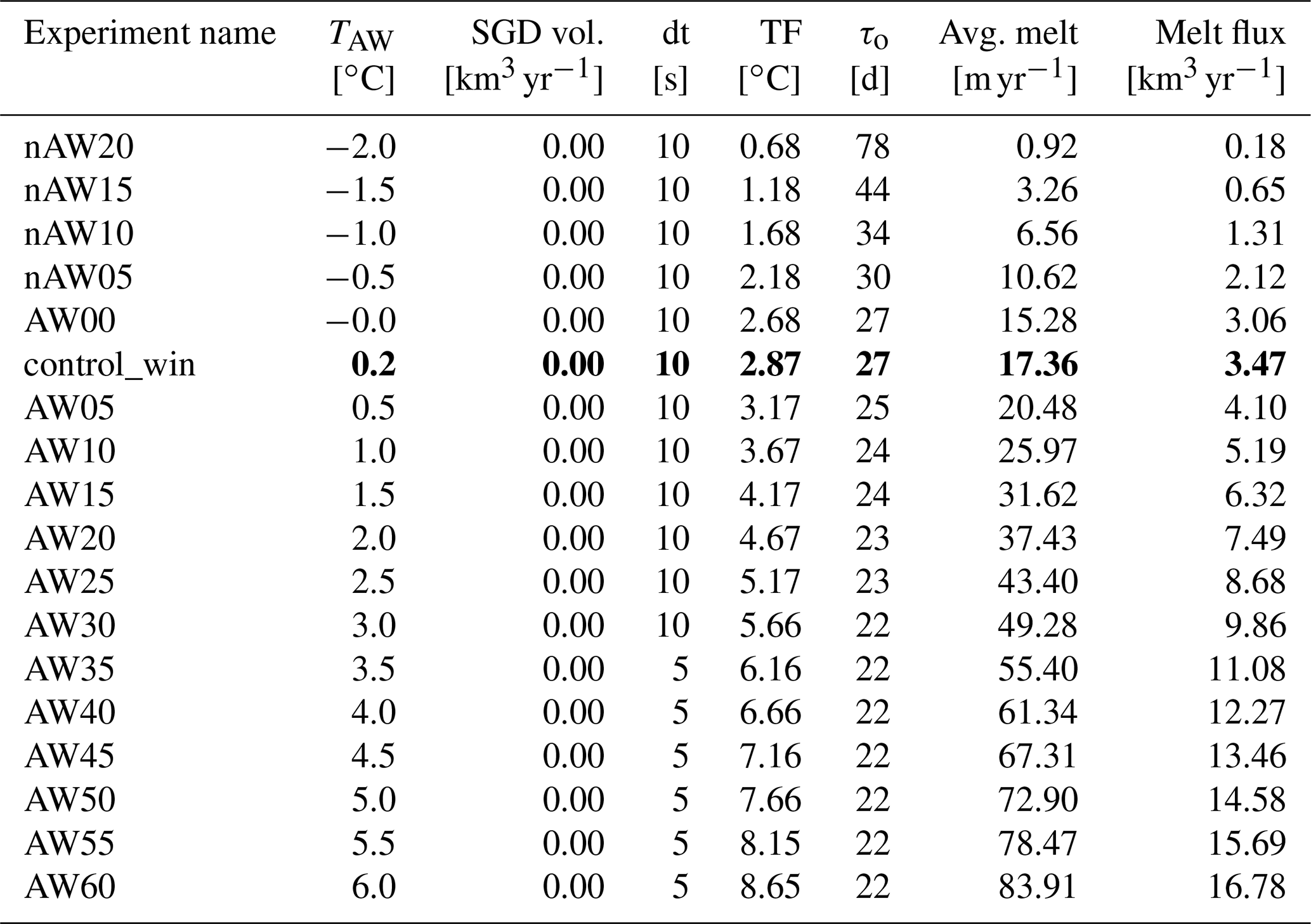
Table A2 Setup parameters and characteristic diagnostics for subglacial discharge sensitivity experiments. From left to right, Atlantic Water Temperature, subglacial discharge volume in percent of control_win integrated melt volume, model time step, TF, overturning timescale, averaged melt rate and integrated melt for a 10 km wide fjord. Values from the winter and summer control simulations are highlighted in bold.

Appendix B: Supplementary figures

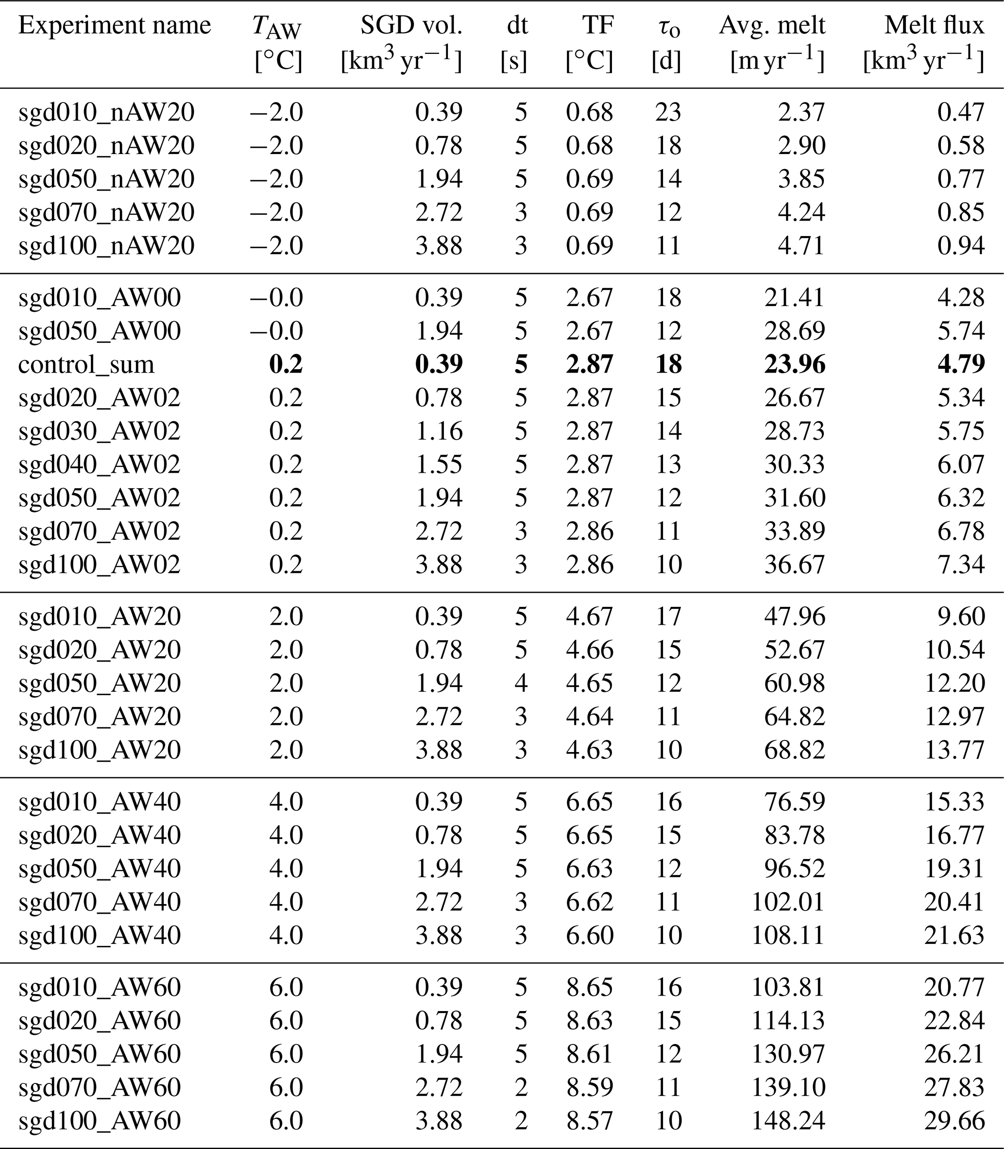
Time series show that for all experiments key diagnostics stabilize after 20–40 d (Figs. B1 and B2). Only the integrated temperature change is increasing with time for high AW temperature experiments after an initial strong decrease (Fig. B1). This increase can be attributed to a heating up of the upper layer of polar water from below. Because all other diagnostics show a statistical steady state, we can assume that the increase in heat does not influence the circulation we are investigating.

Figure B3 shows in colours the buoyancy (a) and velocity (b) in the plume of the control_win simulation. The white line indicates the isoline of the 75th percentile of buoyancy. Compare to Sect. 3.1

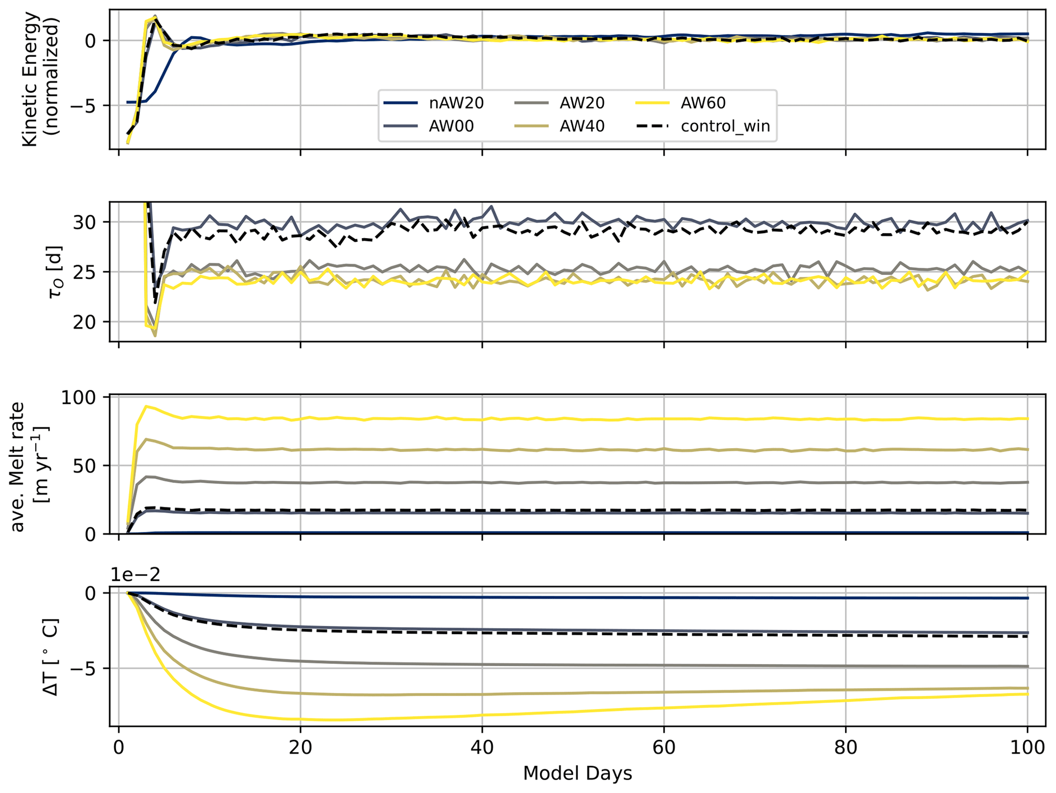
Figure B1 From top to bottom, normalized kinetic energy, overturning timescale, melt rate and integrated temperature change (compared to initial state) as functions of model days; shown for a representative subset of temperature sensitivity experiments.

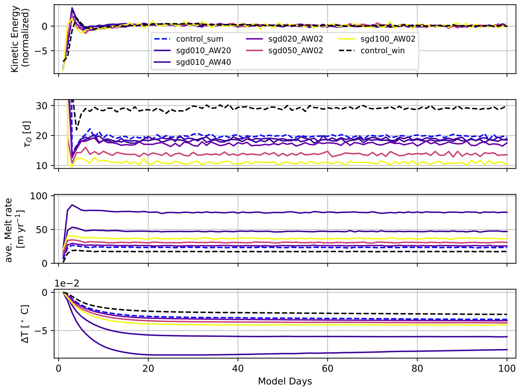
Figure B2 From top to bottom, normalized kinetic energy, overturning timescale, melt rate and integrated temperature change (compared to initial state) as functions of model days; shown for a representative subset of temperature sensitivity experiments.

Figure B3 Section of buoyancy (a) and along-ice velocity (b) within the plume region, as defined by the horizontal velocity criterion (u > 0). The white lines indicate the 75th percentile buoyancy isoline.