the Creative Commons Attribution 4.0 License.
the Creative Commons Attribution 4.0 License.
 | 11 Jul 2023
Underestimation of oceanic carbon uptake in the Arctic Ocean: ice melt as predictor of the sea ice carbon pump
Katja Fennel
Eric C. J. Oliver
Michael D. DeGrandpre
Timothée Bourgeois
Xianmin Hu
Youyu Lu
The Arctic Ocean is generally undersaturated in CO2 and acts as a net sink of atmospheric CO2. This oceanic uptake is strongly modulated by sea ice, which can prevent air–sea gas exchange and has major impacts on stratification and primary production. Moreover, carbon is stored in sea ice with a ratio of alkalinity to dissolved inorganic carbon that is larger than in seawater. It has been suggested that this storage amplifies the seasonal cycle of seawater pCO2 and leads to an increase in oceanic carbon uptake in seasonally ice-covered regions compared to those that are ice-free. Given the rapidly changing ice scape in the Arctic Ocean, a better understanding of the link between the seasonal cycle of sea ice and oceanic uptake of CO2 is needed. Here, we investigate how the storage of carbon in sea ice affects the air–sea CO2 flux and quantify its dependence on the ratio of alkalinity to inorganic carbon in ice. To this end, we present two independent approaches: a theoretical framework that provides an analytical expression of the amplification of carbon uptake in seasonally ice-covered oceans and a simple parameterization of carbon storage in sea ice implemented in a 1D physical–biogeochemical ocean model. Sensitivity simulations show a linear relation between ice melt and the amplification of seasonal carbon uptake. A 30 % increase in carbon uptake in the Arctic Ocean is estimated compared to ice melt without amplification. Applying this relationship to different future scenarios from an earth system model that does not account for the effect of carbon storage in sea ice suggests that Arctic Ocean carbon uptake is underestimated by 5 % to 15 % in these simulations.
- Article
(3087 KB) - Full-text XML
-
Supplement
(3677 KB) - BibTeX
- EndNote


According to current estimates, the Arctic Ocean accounts for 5 % to 14 % of the total global oceanic carbon uptake (Bates and Mathis, 2009; Schuster et al., 2013; MacGilchrist et al., 2014; Yasunaka et al., 2016, 2018). Longer open-water seasons are expected to increase Arctic oceanic carbon uptake in the near term, with complex feedbacks altered by climate change (Lannuzel et al., 2020; Steiner et al., 2015; Ouyang et al., 2020), but the scarcity of biogeochemical observations in the Arctic Ocean prevents reliable calculations of carbon flux (e.g., Landschützer et al., 2014), as well as proper validation of climate models in the region.
In the Arctic Ocean, air–sea gas exchange is mostly prevented by sea ice in winter, while being partially allowed in summer when there is open water. While carbon fluxes between ice and atmosphere are known to exist (Delille, 2006; Miller et al., 2011; Geilfus et al., 2012; Nomura et al., 2010), large uncertainties remain on their significance (Watts et al., 2022), and sea ice is therefore often regarded as a physical lid. Melting and freezing of sea ice affect the partial pressure of CO2 (pCO2) in the surface ocean and thus the air–sea flux, which depends on the pCO2 gradient between the surface ocean and overlying atmosphere (e.g., Wanninkhof, 2014). Melting dilutes dissolved constituents in the surface ocean, thus decreasing dissolved inorganic carbon () and pCO2; the opposite is true when ice is forming (DeGrandpre et al., 2019). Moreover, when sea ice forms, it rejects the dissolved salts in the brine filling the gaps between the crystal lattice. Part of this salty, carbon-rich brine is expelled from the ice (Miller et al., 2011). Sinking of some of this dense brine provides a pathway for carbon export below the mixed layer (König et al., 2018; Barthélemy et al., 2015, and references therein). DIC and alkalinity (here simplified as carbonate alkalinity = ) are also stored inside the sea ice in brine channels. Since alkalinity is retained preferentially (Rysgaard et al., 2007, 2009), this carbon storage in ice affects surface ocean pCO2 during melting and freezing beyond the above-mentioned effects of dilution-, concentration- and brine-driven carbon export.
During ice growth, precipitation of ikaite (hydrated CaCO3) occurs within sea ice: Ca2+ + 2HCO → CaCO3(s) + H2O + CO2(aq) (Dieckmann et al., 2008). This precipitation traps alkalinity inside the ice crystal lattice and increases DIC in the brine (Rysgaard et al., 2009, 2013). Brine drainage then expels part of this DIC, lowering its concentration inside the sea ice, while increasing it in underlying water. Brine drainage also allows for the exchange of nutrients between ice and ocean, feeding sympagic (ice-affiliated) ice algae in spring and further decreasing DIC in ice through primary production (Vancoppenolle et al., 2013). By the end of the ice growth season, the alkalinity to DIC ratio is significantly higher in sea ice than in adjacent seawater. During the melt season, ikaite dissolves in seawater, preferentially releasing alkalinity over DIC, thus further lowering sea surface pCO2 and increasing oceanic carbon uptake (Rysgaard et al., 2012). This process is commonly referred to as the “sea ice carbon pump” (Rysgaard et al., 2007). The intensity of this pump and the underlying drivers are still subject to discussion (e.g., Delille et al., 2014), and the long-term fate of the uptaken carbon is controlled by subduction processes, including advection of water masses to depth (Bopp et al., 2015; Karleskind et al., 2011).
While the role of biotic and abiotic processes in the carbon cycle within sea ice is becoming better understood, their impact on the underlying seawater is less clear. Using a conceptual model, Rysgaard et al. (2011) estimated that the sea ice carbon pump could generate an additional uptake of 50 Tg C yr−1, accounting for 17 % to 42 % of high-latitude carbon uptake. Applying an empirical relationship between CO2 flux and sea ice temperature to a numerical model, Delille et al. (2014) estimate that Antarctic sea ice uptakes 29 Tg C yr−1. In their idealized climate scenarios, Moreau et al. (2016) found that the impact of carbon storage on sea ice weakens the Arctic CO2 sink, while Grimm et al. (2016) suggested a moderate role of the sea ice carbon pump in the modern global carbon cycle but acknowledged its potential importance on regional scales. Finally, in a regional ocean model, Mortenson et al. (2020) showed that the amplitude of the DIC seasonal cycle increased by 25 % in the surface ocean but with an unchanged annual carbon uptake (<1 % increase). The discrepancies between those studies suggest that the importance of carbon storage in ice in the global carbon cycle is still an open question, with increasing relevance due to the current and projected evolution of sea ice.
The sea ice carbon pump is considered to result mostly from three groups of processes: (i) sea ice growth or melt, which implies a freshwater flux (upward or downward) from the ocean to the ice; (ii) brine rejection, which proportionally decreases the uptake of solutes in sea ice; and (iii) active biogeochemical processes, which modify the alkalinity to DIC ratio in sea ice. Most, if not all, earth system models (ESMs) lack a representation of biogeochemical processes within sea ice and are therefore unable to account for (ii) and (iii) but encompass (i) by dilution and concentration of tracers, similar to the handling of precipitation and evaporation. In the present study, we do not distinguish between (ii) and (iii) and instead consider that the carbon cycling in sea ice encompasses both aspects. We also consider our reference point (later referred to as CTRL) to be that of current ESMs; i.e., they include processes (i) but not processes (ii) and (iii).
Arctic sea ice extent and thickness have declined rapidly over the past few decades at a rate of −83 000 km2 yr−1 for September ice extent during the 1979–2018 period and with a decline in ice thickness by 65 % from 1975 to 2012 (Meredith et al., 2019). This decline is expected to continue. Arctic amplification, a combination of positive feedbacks, including summer albedo loss and changes in cloudiness, is leading to twice the rate of warming of the atmosphere compared to the global average (Meredith et al., 2019, Box 3.1). Increased “Atlantification” of the Eurasian Arctic Basin, characterized by a progression of Atlantic water masses into the Arctic seas, is contributing to amplified basal ice melt (Polyakov et al., 2017). These dynamic and thermodynamic processes have direct impacts on sea ice seasonality and extent (Perovich and Richter-Menge, 2009), and ice-free summers are predicted to happen within the next few decades (Overland and Wang, 2013; Notz and Community, 2020). Yet, since sea ice extent in winter decreases slower than in summer, the seasonally ice-covered area is expanding. Such an amplified seasonality in sea ice may intensify the sea ice carbon pump, as sea ice forms in open water that had previously been perennially ice-covered.
We use two independent and complementary approaches to investigate the supplementary carbon flux in the Arctic Ocean. We define the supplementary carbon flux Δℱ as the fraction of the air–sea CO2 flux that is solely due to the storage of carbon and alkalinity in ice. This term is quantified here as the difference in air–sea CO2 flux between a reference situation where there is no ice–ocean carbon flux, i.e., including aforementioned processes (i) but not (ii) nor (iii), and situations where ice–ocean carbon flux occurs, i.e., including (i), (ii) and (iii). First, we combine a set of mathematical formulations to obtain an equation that provides a theoretical framework for the description of the impact of alkalinity and DIC storage in sea ice on air–sea CO2 fluxes. These theoretical considerations suggest that sea ice melt and open-water fraction are the main drivers of an increased oceanic carbon uptake induced by storage of alkalinity and DIC in sea ice. Second, a simple parameterization of the presence of alkalinity and DIC inside the sea ice is implemented in a one-dimensional (1D) ocean model applied to different locations of the Arctic. A large set of sensitivity runs with this 1D model consolidates and expands on the role and importance of melt and open-water fraction and shows that the alkalinity to DIC ratio in sea ice plays a major role in the magnitude of the increased uptake. By forcing the model with a wide range of plausible ice conditions, we obtain a predictive linear relationship between annual ice melt and ice-induced annual supplementary carbon uptake (Δℱ). This relationship can be used to correct carbon uptake estimates from numerical models that do not account for carbon storage in ice. By applying the relationship to an earth system model (ESM) from the sixth phase of the Climate Model Intercomparison Project (CMIP6) ensemble, we show how the impact of sea ice on carbon uptake may evolve under different future emission scenarios.
The impact of carbon storage in sea ice on the air–sea CO2 flux is analyzed using differential equations that account for the impact of freezing and melting on surface water alkalinity and DIC. The air–sea flux is expressed as a function of sea surface pCO2, which depends on temperature, salinity, alkalinity and DIC.
We assume the flux of alkalinity and DIC between the sea ice and the underlying water to be proportional to the freshwater flux induced by freezing and melting of sea ice, (m s−1), and the concentration of alkalinity and DIC inside the ice. The DIC and alkalinity concentrations are assumed to be homogeneous in the ice. The freshwater flux is positive (downward) for melting. The change in sea surface pCO2, written , resulting from the freshwater flux can then be expressed as
with
where H0 is the mixed-layer depth (in m), considered constant for ease of interpretation; [Alk]ice and [DIC]ice are the concentrations of alkalinity and DIC inside sea ice (mmol m−3), and and are the fractional change of pCO2 with alkalinity and DIC, respectively (µatm m3 mmol−1). Note that and are generally non-linear.
The relation between the air–sea flux of CO2 and seawater pCO2 is
where pCO2 and pCO refer to pCO2 in surface seawater and atmosphere (µatm), respectively; kg is the gas transfer velocity (m s−1); is the CO2 solubility (mol m−3 µatm−1); and λ is the fraction of open water (lead fraction, unitless; Ahmed et al., 2019). Here, the air–sea CO2 flux is defined as positive downward.
The supplementary flux, Δℱt, is calculated as the difference between a case with carbon storage in ice, referred to as ICE, and a control (CTRL) case, where storage is not considered, and ice growth or melt only leads to a freshwater exchange, i.e.,
with pCO and pCO being the sea surface pCO2 in the ICE and CTRL cases, respectively. In the rest of this paper, we will denote .
We assume that in both CTRL and ICE cases, sea surface pCO2 experiences the same alterations due to biological processes and changes in temperature and salinity caused by vertical and horizontal mixing and air–sea ice interactions. This assumption neglects the possibility that non-linearities of the carbonate system lead to differences in the impact of these processes on pCO2 between the CTRL and ICE cases. Moreover, we assume that is constant. Calculations conducted with CO2SYS (Lewis and Wallace, 1998) based on mooring data located in the Beaufort Gyre (DeGrandpre et al., 2019; 78∘ N, 150∘ W) and our model data (see Beaufort Gyre setup in Sect. 3.1) yield a coefficient of variation of of only 6 % and 5 %, respectively. This supports the assumption of a constant over the range of expected DIC. These two assumptions are only used in this theoretical derivation, not in the numerical analysis.
The change of pCO2 over time can be written as
with the temperature and salinity contributions (the last two terms on the right-hand side) being identical in the ICE and CTRL cases.
The contributions from alkalinity and DIC can come from advection, diffusion, mixing, biological processes (production, respiration, remineralization), and air–sea or ice–ocean carbon fluxes. As already described, the ice–ocean carbon flux modifies the surface seawater pCO2, which in turn impacts the air–sea carbon flux. Here, the ice–ocean and air–sea carbon fluxes are the two only processes that are not considered identical between CTRL and ICE cases and are therefore the only two terms left when subtracting the equations for for the CTRL and ICE cases from each other. The following differential equation governing the evolution of can be derived (see details in the Supplement):
The solution to Eq. (3) is
where A(t) is a primitive of , and s is the variable of integration, with units of seconds. The primitive of a function can be calculated as its time integral plus an unknown constant α:
This yields a solution for the instantaneous difference in pCO2 between CTRL and ICE scenarios. To retrieve the previously defined supplementary carbon uptake, i.e., the cumulative air–sea CO2 flux that is induced by the pCO2 change, we can insert Eq. (4) into the left-hand side of Eq. (3) and integrate over a period T
A unique derivation to our knowledge, this formulation is composed of three main terms: g(t), which is a function of the concentration of alkalinity and DIC in the ice (Eq. 1); the freezing–melting flux ; and the more complicated exponential of the primitive, which contains the lead fraction λ in A(t). A(t) is an integral of the lead fraction and can be interpreted as keeping a memory of the evolution of the ice conditions.
The sign of g(t) determines the sign of Δℱt. Using realistic alkalinity and DIC values for the Arctic Ocean (e.g., [Alk]sw = 2300 mmol m−3, [DIC]sw = 2100 mmol m−3, [Alk]ice = 540 mmol m−3 and [DIC]ice = 300 mmol m−3, as in Rysgaard et al. (2011) and Miller et al. (2014) or [Alk]ice = 415 mmol m−3 and [DIC]ice = 330 mmol m−3, as in DeGrandpre et al. (2019); and Revelle and alkalinity factors of 14 and −13.3, respectively, as in Takahashi et al., 1993) yields a negative sign for g(t). It can be shown that the term between parentheses in Eq. (5) is always negative, meaning that for ice melt (), Δℱt is downward (uptake); the opposite is true for ice formation (see Supplement). According to this formulation, the dependency of Δℱt on [Alk]ice and [DIC]ice is bi-linear due to the shape of g(t).
It is important to note that the gas transfer velocity and the CO2 solubility, used in the primitive A(t), require no assumption of shape or value. The gas transfer velocity kg can depend on the wind speed (e.g., Wanninkhof, 2014), the wave slope (Bogucki et al., 2010), or turbulence generated by ice drag and convection (Loose et al., 2014). Similarly, the CO2 solubility could follow Weiss (1974) or any other expression.
One can calculate the solution numerically using the carbonate properties of seawater and sea ice (i.e., their alkalinity and DIC), sea ice concentration, ice–ocean freshwater flux, gas transfer velocity (e.g., using Loose et al., 2014) and CO2 solubility (which depends on temperature and salinity; Weiss, 1974). The product of the Schmidt number and CO2 solubility can reasonably be considered constant (Etcheto and Merlivat, 1988), therefore removing the dependency on temperature and salinity (Wanninkhof, 2014, their Eq. 6) and providing an even simpler form than proposed above.
In order to interpret the role of λ, its value can be constrained as follows. We assume that ice formation is associated with full ice cover (λ≈0) and that melting occurs in open waters (λ≈1). We will see that this is supported by ocean model output in Sect. 4.1. Then, during ice formation when λ is very small, .
This implies that the integrand in Eq. (5) is negligible during freezing and non-negligible during melting. Thus, ice formation has a relatively small contribution to the temporal integral of the supplementary carbon flux, while ice melting significantly increases the CO2 flux. Since melting leads to uptake, according to the sign examination above, the net outcome of the supplementary carbon flux is uptake.
Note that if H0 was assumed to be variable in time, it would remain inside the integrands on both sides of Eq. (5). The integrand is then likely to be small during the melting season when the mixed layer shoals and larger during the freezing season, when λ is close to 0 and the integrand is already small. A variable mixed-layer depth would therefore reinforce the already dominant influence of the melting season in the value of the supplementary carbon uptake.
We implemented a parameterization of carbon storage and release by sea ice in a 1D ocean model, independently of the theoretical arguments in Sect. 2, to investigate its impact on the air–sea CO2 flux in different regions of the Arctic Ocean. We do not use any of the results or assumptions from Sect. 2. By using a wide range of initial and forcing conditions derived from a realistic 3D model, a large ensemble of 1D simulations is generated to account for spatial and temporal variability in forcing conditions. Analysis of the ensemble provides insights into the main drivers of the supplementary carbon uptake and allows us to derive a formula to estimate the supplementary carbon flux in existing earth system model (ESM) simulations. Here we describe the 1D model setup and forcings, as well as the ESM outputs, used to project the evolution of the supplementary carbon flux in different scenarios.
3.1 1D ocean model
The 1D General Ocean Turbulence Model (GOTM; Burchard et al., 1999; Umlauf and Burchard, 2005; Umlauf et al., 2014; see https://gotm.net, last access: 13 December 2019) is coupled to the Pelagic Interactions Scheme for Carbon and Ecosystem Studies volume 2 (PISCES-v2; Aumont et al., 2015), specifically adapted to the Framework for Aquatic Biogeochemical Models (FABM; Bruggeman and Bolding, 2014). The vertical grid has fixed layer thicknesses, with a resolution of 1 m near the surface and increasing with depth (9 layers in the first 10 m, 24 layers in the first 100 m). Air–sea CO2 flux is calculated by the model using values from Wanninkhof (2014) with 10 m wind speed. The carbonate chemistry in the model follows the OCMIP protocols (Orr, 1999).
The evolution of alkalinity and DIC in surface waters is parameterized by
where the first term on the right-hand side describes the ice–ocean carbon flux, with [Alk]ice and [DIC]ice being the alkalinity and DIC concentrations in ice and held constant throughout a simulation; is the flux of freshwater between ice and the ocean due to ice melt or freezing (m s−1; positive downward); Hcell is the thickness of the uppermost ocean grid cell (here 1.02 m); Phys includes the dispersive transport terms as well as dilution and concentration due to sea ice melting and freezing or due to precipitation and evaporation; Bio represents the biological sources and sinks of Alk and DIC; and is the air–sea CO2 flux. Preliminary runs showed that the biological terms have a similar impact on carbon uptake regardless of whether the carbonate system inside sea ice is represented or not and thus yield a negligible impact on supplementary carbon uptake (less than 1 % normalized difference). They were therefore deactivated for the ensemble runs to save computational effort.
Surface forcings were prescribed from a 3D physical–biogeochemical–ice–ocean model based on NEMO-LIM-PISCES (Madec et al., 2017; Rousset et al., 2015; Aumont et al., 2015) for the North Atlantic, North Pacific and Arctic oceans, hereafter referred to as the NAPA model. The NAPA model, including the validation with observational data, is documented in Zhang et al. (2020) and Zheng et al. (2021). In our application of this 3D model, the atmospheric forcing was obtained from the ERA5 reanalysis product (Hersbach et al., 2020) from 2014 to 2019. Outputs were written out daily, providing the necessary temporal resolution to capture sub-seasonal variability. We used the simulated ice concentration, latent and sensible heat fluxes, longwave and shortwave radiative fluxes, freshwater fluxes (due to ice melt–freeze and evaporation–precipitation), and momentum fluxes (due to wind and ice drift) at the top of the surface layer of the model, calculated as a weighted average between open water and under ice conditions to force the 1D model. This methodology allows us to simulate the impact of sea ice in our 1D model without having to resort to a full ice component. Other inputs necessary for air–sea CO2 flux include the wind speed and mean sea-level pressure from ERA5, as well as atmospheric pCO2 from the Alert Station, Northwest Territories of Canada (Keeling et al., 2001).
In generating the ensemble of 1D simulations, every 10th horizontal grid cell of the NAPA domain was selected with the following exceptions. Since our focus is on open-ocean conditions with a significant presence of sea ice, coastal locations with water depths shallower than 100 m as well as the Canadian Arctic Archipelago, Hudson Bay and the Baltic Sea were excluded. Also excluded were grid cells with both ice melt and freezing rates of less than 0.1 m yr−1. Given NAPA’s average grid spacing of 12 km in the Arctic, every 10th grid cell leads to roughly one cell every 120 km for a total of 732 cells, covering a wide range of ice conditions. For each of these locations, we ran the 1D model for six 1-year simulations starting on 1 January for the years 2014 to 2019, with initial conditions from the NAPA model. Since the 1D model cannot explicitly represent horizontal advection, its solutions were nudged toward the properties simulated by the NAPA model with a timescale of 4 months for temperature and salinity and 1 year for alkalinity and DIC. As a consequence, subduction processes are mostly but not entirely neglected in this 1D model.
Based on the above setup, we systematically ran the 1D model in two configurations CTRL (no carbon in sea ice) and ICE (storage of carbon in sea ice). In both configurations, sea ice growth and melt generate a freshwater flux that concentrates or dilutes tracers at the surface ocean. The runs are listed in Table 1. The supplementary carbon uptake Δℱm is calculated as the difference in annual air–sea CO2 flux between the ICE (or ICE2) and the CTRL runs. We consider the air–sea CO2 flux in the CTRL run as the baseline, since it corresponds to the values reported by numerical models that do not account for the sea ice carbon pump. Potential predictors of the supplementary carbon flux are investigated, including the net freezing–melting flux (the integral over a year of the freshwater flux between ice and ocean); the gross melting (freezing) flux, which only accounts for ice melt (formation); and the yearly integrated ice concentration (which ranges between 0 and 365). We binned the latter metric into nine bins of equal size and applied a linear regression between gross annual ice melt and the supplementary carbon uptake for each of these bins, which can be considered different ice regimes.
Table 1Description of 1D model runs. For more in-depth sensitivity experiments (*), we selected a representative station in the Beaufort Gyre (78∘ N, 150∘ W) for the years 2014 and 2015, where mooring observations are available (DeGrandpre et al., 2019; see comparison in the Supplement). n/a signifies not applicable.
3.2 Application to an earth system model
ESM output from the CMIP6 suite of models can be used to estimate the supplementary carbon flux in projected future climate scenarios. We chose the ACCESS-ESM1.5 model (Ziehn et al., 2020) because it has a plausible simulation of sea ice (according to Notz and Community, 2020), and its monthly averaged freshwater ice–ocean flux due to ice thermodynamics (CF standard name: fsitherm) and air–sea CO2 flux (CF standard name: fgco2) are available. The horizontal resolution of the ocean component of ACCESS-ESM1.5 is 1∘, with 50 vertical levels. The historical simulation covers 1850 to 2015, and three available Shared Socio-economic Pathway (SSP) scenarios (SSP1-2.6, SSP2-4.5 and SSP5-8.5) cover the period from 2015 to 2100. Monthly outputs of the freshwater ice–ocean flux and air–sea CO2 flux were extracted for the historical simulation and the three SSP scenarios.
Consistent with the methodology applied to our 1D model study, only grid cells where ice melt or freeze was over 0.1 m yr−1 were used. For each year between 1850 and 2100 and each remaining grid cell, ice–ocean freshwater flux was summed for melting months only (thus excluding negative values of fsitherm).
4.1 Ensemble of 1D model experiments
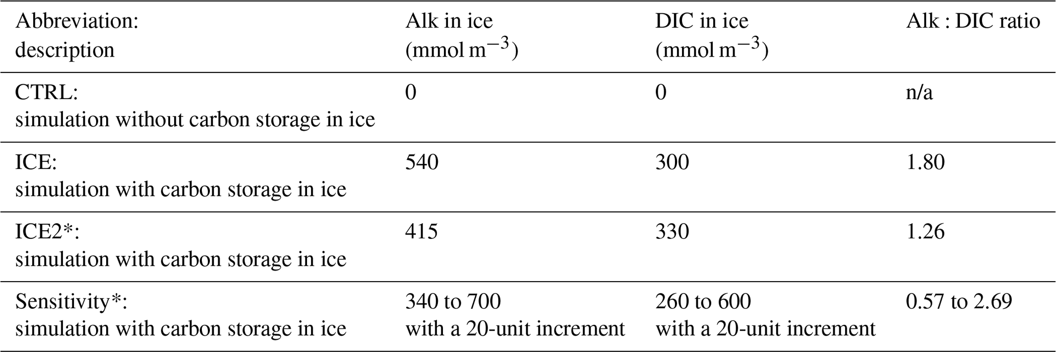
In the CTRL run (no ice–ocean carbon flux), pCO2 increases to maxima of 347 and 354 µatm in the winters of 2014 and 2015, respectively, due to the removal of freshwater and associated concentration of DIC and alkalinity (Fig. 1c). The pCO2 decreases to minima of 305 and 265 µatm in the summers of 2014 and 2015, respectively, when ice melts and dilutes seawater constituents. In the ICE run, when accounting for the ice–ocean carbon flux, the seasonal cycle of pCO2 is similar but amplified, reaching higher maxima (360 and 375 µatm in 2014 and 2015, respectively) and lower minima (254 and 153 µatm in 2014 and 2015, respectively).
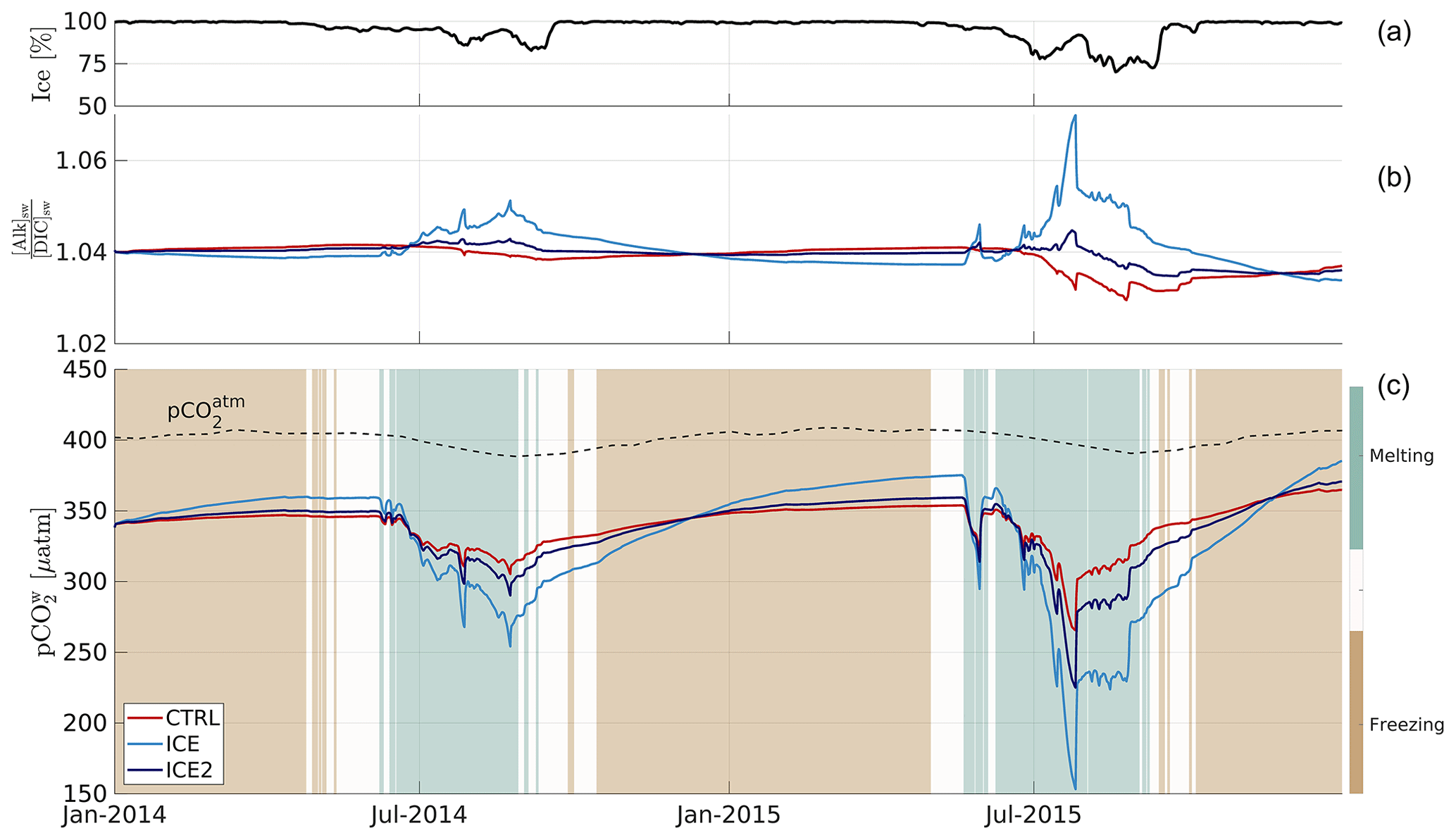
Figure 1Model outputs for a grid cell representative of central Beaufort Gyre (78∘ N, 150∘ W) over 2014–2015. (a) Ice concentration. (b) Surface seawater alkalinity to DIC ratio for the CTRL (no ice–ocean carbon flux; red line), ICE ([Alk]ice = 540 mmol m−3, [DIC]ice = 300 mmol m−3 ; light blue line) and ICE2 ([Alk]ice = 415 mmol m−3, [DIC]ice = 330 mmol m−3; dark blue line) runs. (c) Ice melt and formation (>3 mm d−1; background colour), observed atmospheric pCO2 at the Alert weather station (dashed black line), and simulated surface seawater pCO2 (solid lines) for the three above-mentioned runs.
The reason for this amplification is illustrated in Fig. 1b. When accounting for the ice–ocean carbon flux, the alkalinity to DIC ratio at the surface decreases during the freezing season and increases during the melting season, a behaviour that is opposite to the control run. Since an increase in alkalinity decreases pCO2, and an increase in DIC increases pCO2, the storage and release of both properties by sea ice have counteracting effects. The alkalinity effect dominates and leads to a decrease in seawater pCO2 when ice melts, amplifying the seasonal cycle of pCO2. The degree of amplification depends on the values of [Alk]ice and [DIC]ice, as illustrated by comparing the ICE and ICE2 runs with different alkalinity to DIC ratios of the ice–ocean carbon flux. ICE2, which has a lower alkalinity to DIC ratio (1.26 compared to 1.80 for ICE), shows lower maximum values (350 and 359 µatm in 2014 and 2015, respectively) and higher minimum values (290 and 225 µatm in 2014 and 2015, respectively) of pCO2 compared to ICE.
How this amplification of the seasonal cycle of pCO2 affects the seasonal air–sea CO2 flux depends on the ice cover shown in Fig. 1a. According to the formulation in Eq. (2), almost complete ice cover (λ=0) in winter results in an air–sea CO2 flux close to 0 when pCO2 is the highest. Lower sea ice cover in summer allows for some air–sea gas exchange directly proportional to the air–sea pCO2 gradient. Integrated over a full seasonal cycle, the amplification of the pCO2 cycle results in net oceanic CO2 uptake added to the baseline. In the case of the Beaufort Gyre station location, averaged over both years, this supplementary uptake Δℱm amounts to 45.5 mmol C m−2 yr−1 for an alkalinity to DIC ratio of 1.80 (ICE) and 13.6 mmol C m−2 yr−1 for a ratio of 1.26 (ICE2), over a 3-fold difference. Note that these are low flux values relative to other oceans (usually higher than 1 mol C m−2 yr−1), mainly because of the ice cover.
The effect of carbon storage on the annual net CO2 flux is explored more thoroughly for the Beaufort Gyre location by varying [Alk]ice from 340 to 700 mmol eq. m−3 and [DIC]ice from 260 to 600 mmol m−3 (Fig. 2). The net CO2 flux (Fig. 2a) and supplementary carbon uptake Δℱm (Fig. 2b) are strongly dependent on the alkalinity to DIC ratio in ice (white contours). Notably, the net CO2 flux varies by a factor of 2 to 3 for realistic values of the alkalinity to DIC ratio. Thus, alkalinity and carbon storage in ice have a significant impact on the net air–sea CO2 flux in the model.
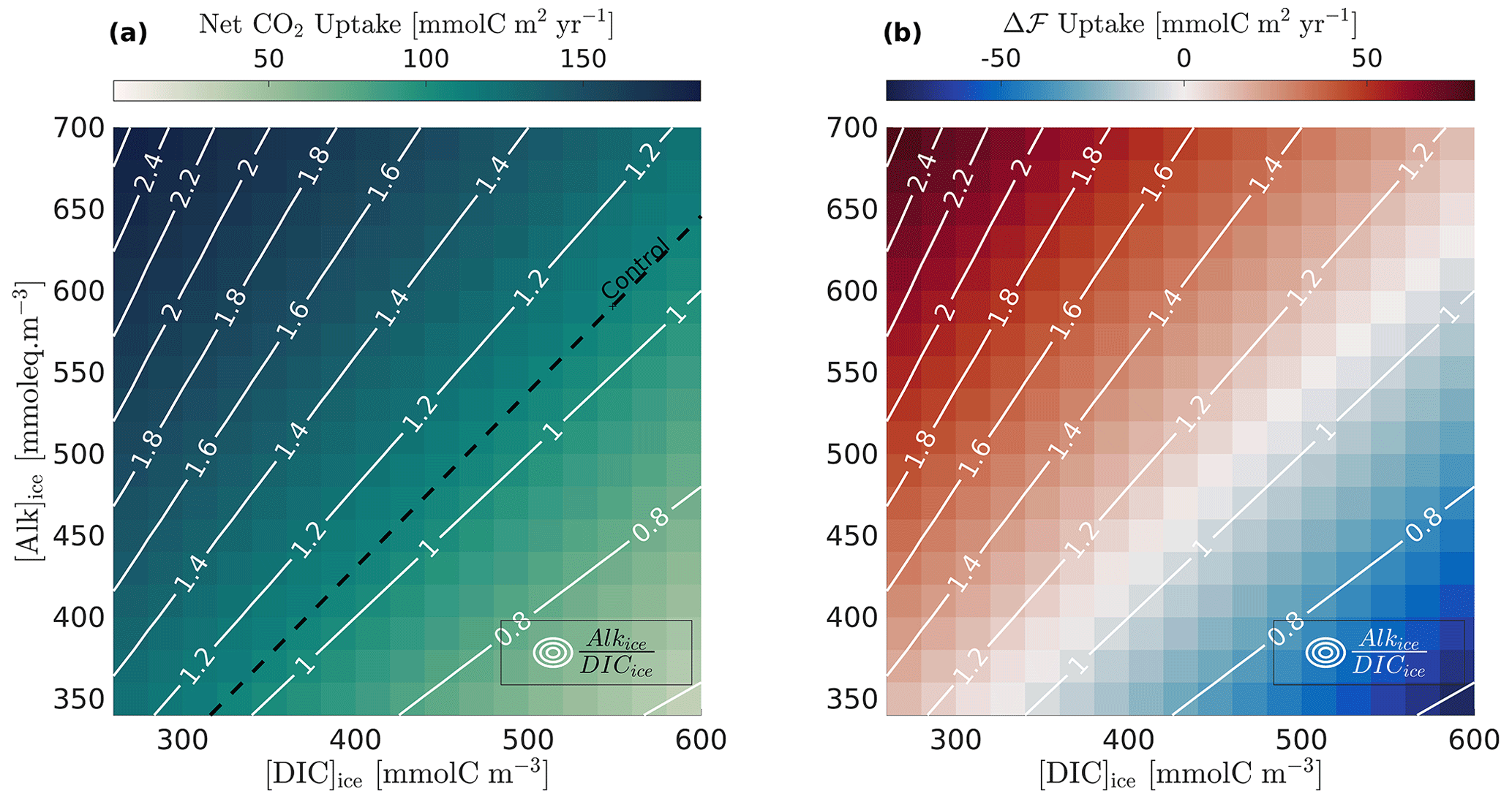
Figure 2Dependence of annual net CO2 uptake on alkalinity and DIC concentrations in ice. The two panels show results from model sensitivity runs for a wide range of alkalinity and DIC values in ice (20-unit increments). (a) Annual net CO2 uptake (background colours); the net CO2 uptake value for the standard run is highlighted by the dashed black line for reference (note that the standard run is not a part of the runs shown in the background colours, since [Alk]ice = [DIC]ice = 0). (b) Supplementary carbon flux Δℱm due to carbon storage in ice (background colours). The ALK:DIC ratio in ice is superimposed (white lines).
Next, we investigate the role of ice conditions, including the freezing–melting rate, and ice concentration in the air–sea CO2 flux. The NAPA model simulates a wide range of ice melt rates over the Arctic Ocean, spanning from 0 to over 7 m yr−1 and with areas of high ice melt in the Labrador and East Greenland currents and the southern edge of the Beaufort Gyre (Fig. 3a). The NAPA model also simulates freezing conditions that mostly occur when the lead fraction is close to 0 (Supplement, Fig. S2). Indeed, over 88 % of the freezing days occur when the ice concentration is above 0.9. This supports the assumption made in Sect. 2, where we considered freezing to mostly occur when the lead fraction is close to 0.
Figure 3Region of interest and sea ice regime from the NAPA model domain. Each dot gives the location of the forcing conditions used to force the 1D model in this study. (a) Mean gross annual ice melt. (b) Mean yearly temporal integral of ice concentration. The red dot shows the grid cell used for Figs. 1 and 2.
Gross freezing rates and yearly integrated ice coverage are poorly correlated to Δℱm (r2 = 0.12 and r2 = 0.15, respectively). Yearly net freezing–melting is more strongly correlated with Δℱm (r2 = 0.39). However, a better Δℱm is ice melt, excluding any freezing, hereafter gross annual melt (r2 = 0.86; Fig. 4). An explanation for this strong relation is that winter ice cover prevents air–sea flux during the freezing period. This is an independent confirmation of the interpretation of the mathematical derivation made in Sect. 2.
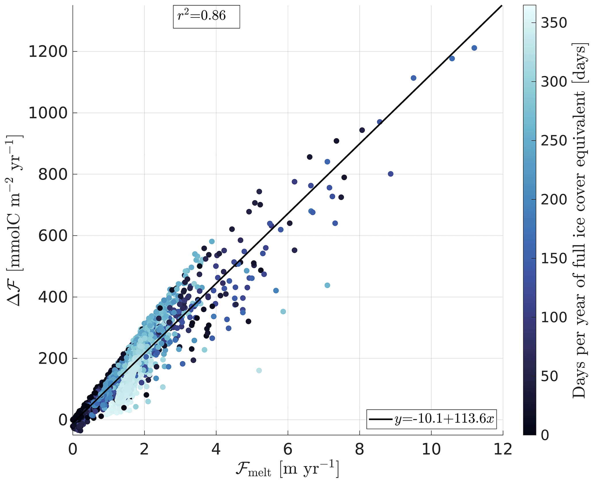
Figure 4Scatterplot of the 1D Arctic-wide runs. The supplementary carbon uptake Δℱ is plotted as a function of the gross annual ice melt. The colour of the dots shows the temporal integral of ice melt over the year, in days. The squared correlation coefficient r2 between both variables is given in the top left corner.
The high correlation between the gross annual ice melt (ℱMelt) and Δℱm gives confidence in a linear model relating those two metrics:
Another driver for Δℱm is the yearly integrated ice concentration (Fig. 4, colours), which is the largest where full ice cover persists for most of the year (Fig. 3b). While model experiments with lower ice coverage (dark blue) follow the regression well (solid black line), runs with higher ice coverage (light blue) have a steeper slope.
The 1D simulation ensemble can be used to calculate a yearly Arctic-wide increase due to ice–ocean carbon flux, for the 2014–2019 period. The ICE runs represent an increase of 30.0 ± 9.1 % (mean ± standard deviation calculated over the 6-year period) compared to the CTRL runs. Equation (6) depends on the parameterization of the carbon ice–ocean flux and air–sea CO2 flux but is not otherwise model-specific. Therefore, it can be applied to other model outputs.
4.2 Application to an earth system model
The amplification of the air–sea CO2 exchange due to the storage of carbon and alkalinity in ice is sensitive to the gross annual ice melt and the seasonality of the ice concentration. Both parameters are rapidly changing due to global warming. To investigate the impact of these changes on the supplementary carbon uptake, we turned to outputs from ACCESS-ESM1.5 (Ziehn et al., 2020). This model, as any ESM, does not include any carbon storage in sea ice, although the freshwater flux between the ocean and sea ice is accounted for. We applied the linear relation in Eq. (6) to estimate the missing carbon uptake of CO2 and, by adding it to the modelled carbon uptake, provided a corrected estimate of the oceanic carbon uptake in polar regions. While subduction processes are simulated in the initial outputs, our offline methodology does not correct mixing and advective carbon transport for the supplementary carbon due to the sea ice carbon pump. Therefore, an inherent assumption to our methodology is the subduction of all the added carbon.
Although the linear relation between gross annual melt and Δℱm (Eq. 6) was derived from daily data, a very similar relationship is obtained when monthly data are used instead (RMSE between daily vs. monthly calculated gross annual ice melt <0.06 m yr−1, not shown), giving us confidence that Eq. (6) can be used. The linear relation was applied to the extracted gross ice melt, resulting in a yearly supplementary carbon uptake for each grid cell. Spatially integrated over the area of interest, this yields an Arctic-wide supplementary carbon uptake due to ice–ocean carbon flux, which can then be added to the model-derived carbon flux over the same area to between Δℱm and the model-derived carbon flux, expressed as a percentage, allows for easier interpretation of the magnitude of the process. This ratio can be interpreted as a measure of how much the ESM underestimates the Arctic Ocean carbon uptake. Those metrics were integrated over the different periods, yielding cumulative carbon uptake estimates over the historical and projection periods.
Due to the CO2 undersaturation of the Arctic Ocean, the net carbon flux is positive (into the ocean) for all periods and scenarios. During the historical run, the modelled uptake slowly increases from 180 Tg C yr−1 in 1850 to 200 Tg C yr−1 in 1995 (a linear regression gives a slope of 0.26 Tg C yr−2 with r2=0.5, p value <0.001), then stagnates during the last 20 years (r2=0.0, p value = 0.4) (Fig. 5a). The supplementary carbon flux, on the other hand, remains relatively constant over the whole period (Fig. 5a), meaning the corrected carbon uptake (Fig. 5a) follows a similar pattern as the model estimate. It also leads to a slow decrease in the ratio of Δℱm over the model estimate (Fig. 5b). The increase in uptake may be driving increasing pCO2 levels in the Arctic Ocean (Ouyang et al., 2020; DeGrandpre et al., 2020).
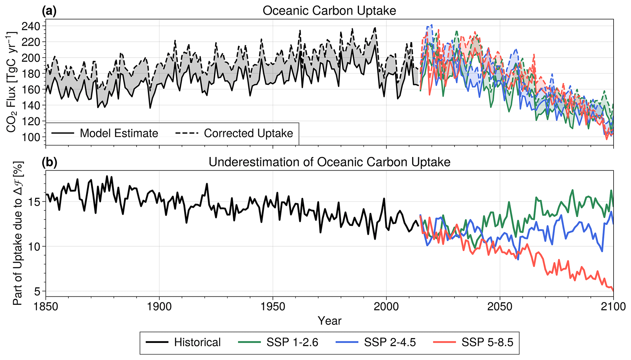
Figure 5Correction of ACCESS-ESM1.5 arctic carbon uptake by applying the linear relation to model outputs, for historical (black), SSP1-2.6 (green), SSP2-4.5 (blue) and SSP5-8.5 (red) scenarios. (a) Arctic oceanic carbon uptake from ACCESS-ESM1.5 (solid lines) and corrected estimates (dashed lines). The shaded area between lines corresponds to the supplementary carbon uptake Δℱm (b) Ratio of Δℱm to model-derived carbon flux, expressed in percentage. This gives an estimate of how much the ACCESS-ESM1.5 model underestimates Arctic oceanic carbon uptake due to the lack of parameterization of ice–ocean carbon flux.
Projecting into the future, all three climate scenarios show a decrease in modelled and corrected carbon uptakes, although interannual variability is high. In scenario SSP5-8.5 (Fig. 5a) and SSP1-2.6 to a lesser extent (Fig. 5a), carbon uptake increases until the 2040s, before dropping rapidly during the remainder of the century. The severe sea ice decline in SSP5-8.5 leads to a similar decrease in Δℱm, while the two other scenarios show a relatively constant Δℱm over the 21st century.
Those scenarios differ in how large the fraction of Δℱm is compared to the total carbon uptake (Fig. 5b). Over the historical period, it slowly decreases, starting above 15 % to arrive at around 12.5 % in 2015. It keeps decreasing in SSP5-8.5 to reach 5 % in 2100, but the other scenarios show a different story, levelling off at around 11 % in SSP2-4.5 and returning to 15 % in SSP1-2.6.
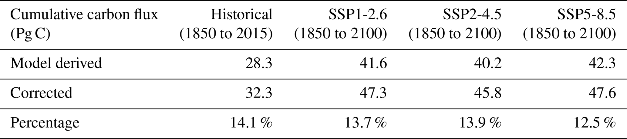
Integrated over 1850–2100, the modelled carbon uptake sums up to 41.6, 40.2 and 42.3 Pg C for scenarios SSP1-2.6, SSP2-4.5 and SSP5-8.5, respectively, and the supplementary carbon uptake adds another 5.7, 5.6 and 5.3 Pg C, respectively (Table 2). Those cumulative supplementary carbon fluxes represent 12.5 % to 14.1 % of the model-derived cumulative flux (Table 2).
Table 2Cumulative carbon uptake from the ACCESS-ESM1-5 model outputs, for historical (black), SSP1-2.6 (green), SSP2-4.5 (blue) and SSP5-8.5 (red) scenarios. Corrected refers to the carbon uptake calculation while taking account of sea-ice-induced supplementary carbon uptake as calculated using our linear regression (Eq. 6). Percentage refers to the normalized difference (in %) between the model-derived and corrected cumulative carbon flux.
Therefore, discarding the storage of carbon in sea ice in ESMs can lead to a significant underestimation of the carbon uptake in the Arctic Ocean, with varying impacts depending on the scenario considered, as described in the Discussion.
In this study, the link between ice–ocean and air–sea carbon fluxes was investigated using two independent methods: a theoretical framework and numerical modelling. The methods provide consistent, complementary results, both pointing to a linear relationship between Δℱ and ice melt and an exponential relation with the open-water fraction (Eq. 5 and Fig. 4).
Only three assumptions were made during the theoretical derivation. The assumption of a constant was addressed in Sect. 2. The second assumption was a constant value of the mixed-layer depth H0, also discussed in Sect. 2. The third assumption is the negligible effect of non-linearities in the carbonate system. Here, it is worth noting that the 1D numerical model does not rely on those assumptions and accounts for the varying and H0, as well as for the non-linearities of the carbonate system. Therefore, the good agreement between the theoretical framework and the model ensemble results builds confidence that these assumptions are justified. Back-of-the-envelope calculations using typical orders of magnitudes (pCO2 = 350 µatm, changes in pCO2 = 20 µatm) also show that non-linearities would represent less than 10 % of the total changes induced by the temperature, salinity, DIC and alkalinity variations, further supporting our assumptions.
A simplified version of the theoretical Eq. (5) can be evaluated with g and considered constant (see Supplement, Sect. S1.4) to better compare both methods. The ice concentration and freezing–melting flux used to force the 1D model (described in Sect. 3.1) can then be applied to this simplified version to calculate Δℱt (Fig. 6). While the constant values and the offline calculations of Δℱt prevent a quantitative comparison with Δℱm shown in Fig. 5, both methods provide a consistent qualitative behaviour, with a clear linear relationship between ℱMelt and Δℱ, and an increasing slope with increasing ice cover.
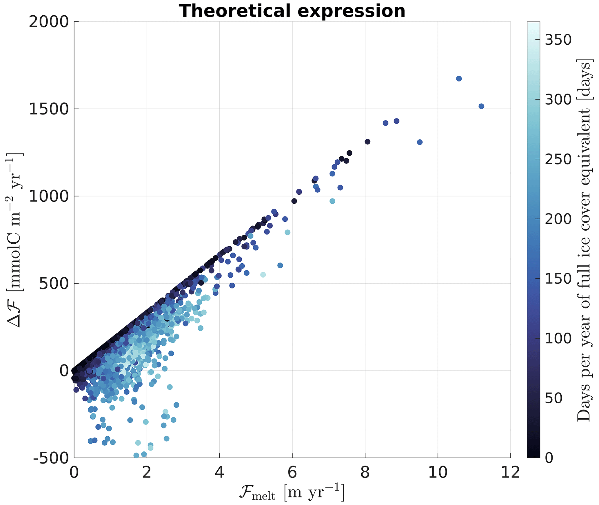
Figure 6Evaluation of a simplified version of Eq. (5) with the 1D model forcings: g(t) and are considered constant at −315 µatm and 0.073 (see Supplement). The general shape of the scatterplot shows reasonable agreement with the online calculation of the supplementary carbon flux shown in Fig. 4.
To interpret the relatively complex equation obtained in the theoretical framework (Eq. 5), we considered that ice formation is associated with ice-covered waters, related to the exponential term. Again, this simplification is supported by results from the NAPA model (see Sect. 4.1 and Supplement Fig. S2). The functional form may not apply to some regions with distinct ice regimes, including ice-exporting polynyas and ice-importing marginal ice zones. In those regimes, the exponential term and therefore the slope of the relation between Δℱ and ice melt would be different. However, our solution is applicable to most of the Arctic Ocean.
We presented an approach for how Arctic carbon uptake estimates from ESMs can be corrected using our linear relation between Δℱm and sea ice melt (Sect. 4.2). In doing so, past and potential future impacts of the sea ice carbon pump in the Arctic can be analyzed. Our analysis suggests that uptake due to the sea ice carbon pump increased during the historical period (Fig. 5a) due to longer open-water seasons and increased atmospheric pCO2. This is consistent with observations in the Canadian Arctic where higher pCO2 levels are correlated with low ice extent (DeGrandpre et al., 2020). Because the sea ice carbon pump only applies to the seasonally ice-covered areas, the decline in ice extent translates into a stagnation of the supplementary carbon uptake toward the end of the historical period and decreases during all SSP scenarios (Fig. 5a). In the SSP5-8.5 projection, the inhibition of the impact of carbon storage in sea ice is linked to drastic ice loss and therefore to less ice melt. In SSP1-2.6 and SSP2-4.5, the ice seasonal cycle remains significant, leading to a larger importance of Δℱm.
In all scenarios, except in SSP5-8.5, we deem the current and future role of carbon storage and release by sea ice as non-negligible. Without it, the ACCESS-ESM-1.5 model could be underestimating carbon uptake over seasonally ice-covered areas by 5 % to 15 % or 10 % to 15 % if we exclude SSP5-8.5. Note that this range differs from our calculation using the shorter NAPA model run from 2014 to 2019, in which the supplementary carbon uptake increases the yearly carbon uptake by 30.0 ± 9.1 % (mean ± standard deviation over 6 years). The discrepancy is mostly due to a lower ice melt simulated by the ACCESS model compared to the NAPA model (∼18 % lower), though both models have a reasonable agreement with satellite observations in terms of sea ice extent and concentration. We note that ACCESS-ESM-1.5 is the only CMIP6 model that provided the ice–ocean freshwater flux and air–sea CO2 flux, which are necessary inputs for our parameterization. An extension of this calculation to other ESMs would be possible if suitable output was available for more models.
Our estimated supplementary carbon flux is consistent with numbers given by Rysgaard et al. (2011), who suggested that the sea ice carbon pump could represent 20 % of the air–sea CO2 flux in open Arctic waters at high latitudes. Rysgaard et al. (2011) assumed complete subduction of the brine, while we did not. Our estimates are higher than those from two other modelling studies. Grimm et al. (2016) reported that 7 % of simulated net polar oceanic CO2 uptake is due to the sea ice carbon pump. Moreau et al. (2016) found a weakened Arctic carbon sink when including the sea ice effect. Neither of these two studies assumed complete subduction and rather diagnosed it from their model, finding it to be relatively small. It has previously been suggested that the differences between the estimates of Rysgaard et al. (2011) and Moreau et al. (2016) are due to the different assumptions about subduction. This study does not support that interpretation. While a direct comparison between all those studies is difficult, we suggest that the vertical resolution is crucial for properly resolving the mechanisms at play. The coarse resolutions used by Grimm et al. (2016) and Moreau et al. (2016) (9 and 10 layers in the first 100 m, respectively, compared to 9 layers in the first 10 m in our configuration) prevent them from capturing the shallow summer mixed layer observed in the Arctic. Using the same resolution as Moreau et al. (2016) in our 1D model leads to significant changes in the magnitude of the air–sea flux, either positive or negative depending on whether the mixed-layer depth is under- or overestimated. The importance of high vertical resolution, capable of properly representing the shallow mixed layers in Arctic regions, is not surprising. On top of that, a proper representation of subduction, included in the Grimm et al. (2016) and Moreau et al. (2016) studies but beyond the scope of the present 1D study, would be important to more fully understand the long-term fate of carbon in the global ocean. Yet, in an undersaturated ocean, the amplification of the pCO2 seasonal cycle can in itself explain an increased seasonal carbon uptake. Without any subduction, this would then lead the Arctic Ocean to reach equilibrium with the atmosphere faster than without accounting for the sea ice carbon pump, eventually saturating the surface ocean and reducing the carbon uptake. The output from the ACCESS-ESM1.5 model accounts for subduction, but the fate of supplementary carbon estimated here cannot be determined without a proper coupling of a sea ice biogeochemical component. It is therefore unknown whether, at the decadal timescales considered for that model, carbon flux driven by advection and mixing would proportionally increase and export the supplementary carbon or whether the latter would saturate the surface mixed layer, leading seawater pCO2 to catch up with atmospheric values faster than without accounting for the sea ice carbon pump. Thus, our estimate should be considered an upper bound of the impact of the sea ice carbon pump.
While the amplified seasonal cycle of carbonate properties found in our study agrees well with Mortenson et al. (2020), they suggest a negligible impact of ice–ocean carbon flux on annual oceanic CO2 uptake. A potential source of this disagreement could be their lower alkalinity to DIC ratio in sea ice (1.25 in their study, 1.8 for this study’s reference case). We have shown that the resulting supplementary carbon uptake is sensitive to this ratio (Sect. 4.1 and Fig. 2).
Our parameterization of the alkalinity to DIC ratio may be overly simplistic. First, the vertical profiles of alkalinity and DIC in sea ice, assumed homogeneous here, might be C-shaped to follow salinity profiles, though observations do not necessarily support a vertical heterogeneity (e.g., Miller et al., 2011; Rysgaard et al., 2009). As long as the parameterized values are representative of the freezing and melting ice over a seasonal cycle, we believe that the vertical homogeneity assumption is reasonable. Second, the alkalinity to DIC ratio is known to increase over time. The ratio can change for several reasons: (1) CO2 outgassing from ice to the atmosphere when brine is expelled at the surface (Miller et al., 2011), or when permeability is restored by increasing temperatures in early spring (Delille et al., 2014; Nomura et al., 2010) it decreases DIC, although uncertainties in these fluxes are high (Watts et al., 2022); (2) primary production from ice algae consumes CO2 and nitrate, therefore reducing DIC, while increasing alkalinity (Delille et al., 2007; Rysgaard et al., 2007); and (3) the formation of ikaite crystals trapped in sea ice retains alkalinity, while CO2-enriched brine is exchanged with seawater (Rysgaard et al., 2007, 2009, 2011). However, the main driver of supplementary carbon uptake is sea ice melt, occurring towards the end of the seasonal cycle, when the alkalinity to DIC ratio is expected to be the highest (Sect. 4.1). Therefore, applying a constant, high ratio is likely to best match real conditions while keeping the parameterization in its simplest possible form. Moreover, while the value of 1.8 might seem high, it is within the range of observed values (1 to 2; Miller et al., 2011; Rysgaard et al., 2009, 2011). Nonetheless, a better constraint on this ratio is needed, which requires a proper understanding of the conditions of ikaite formation.
The empirical linear relation determined in Sect. 4.1 (Eq. 6) involves annual ice melt only, to the exclusion of ice formation. Outputs from the 3D numerical ice model show that whenever the freeze–melt rate is negative (i.e., ice is forming), the ice concentration is close to 1, preventing gas exchange. While this might be due to artifacts inherent to numerical models (e.g., lack of resolution of small leads), our linear relation is derived for application on the latter and therefore stands in this context. It should be noted that we excluded shallow shelves from our runs, such as the Laptev Sea shelves. Those areas are highly productive with regard to ice formation in polynyas (exceeding 7 m yr−1; Dmitrenko et al., 2009) and subject to active leads in winter. Therefore, in those regions, during ice formation, carbon storage in sea ice could yield anomalous outgassing, though intense ice formation has also been linked to enhanced CO2 uptakes (Else et al., 2011). Brine sinking in those areas is also significant enough to form deep water masses and is therefore likely to provide a carbon export mechanism over multiyear timescales. Investigating this mechanism would require a fully coupled 3D model.
In this study, a 1D model was used preferentially for computational reasons. This provided more flexibility for parameterization and sensitivity tests and allowed us to generate a large ensemble of simulations, which would be computationally prohibitive with a full 3D model. For the same reason, we disabled the biological processes in our 1D model. It could be hypothesized that respiration will increase pCO2 in winter when ice is acting as a lid, and primary production will lower it in summer, in phase with the chemical process described here, thus further amplifying the sea ice carbon pump. The storage and release of carbon by sea ice complete the picture drawn by the rectification hypothesis (Yager et al., 1995), which assumes that half of the air–sea CO2 exchange that would be occurring in the typically ice-free ocean is cancelled by the presence of sea ice. While this rectification hypothesis is fully applicable in areas of local ice formation and melt, the southern-most areas of our domain of interest (e.g., Labrador Current and East Greenland Current, Fig. 3) only involve melting of advected ice, usually in winter, and are therefore out of phase with the previously described seasonal cycle of pCO2. Melting of advected sea ice would then decrease pCO2 and increase carbon uptake in winter without modifying it in summer. Deep convection events frequently happening in those areas could then have important consequences for the carbon export at depth, but this is beyond the scope of this study.
In this study, we used two independent but consistent approaches, a theoretical framework and numerical models, to explore the effect of storage and release of alkalinity and DIC by sea ice on air–sea CO2 fluxes. Our theoretical derivation and numerical results show that the ice–ocean carbon flux amplifies the seasonal cycle of surface pCO2 in phase with the seasonal cycle of sea ice concentration. This leads to a significant increase in oceanic carbon uptake in seasonally ice-covered areas in the Northern Hemisphere. One of the key findings of this study is that ice melt is a direct driver of the supplementary carbon uptake and can therefore be used to correct carbon uptake estimates. This supplementary carbon uptake accounts for 30 % of Arctic Ocean carbon uptake according to our regional, high-resolution model and for 5 % to 15 % in the global, lower-resolution ACCESS-ESM1.5 model, depending on the chosen scenario.
We also provide two novel relations to estimate the impact of sea ice carbonate on air–sea carbon flux. The first (see Eq. 5 for the full expression of Δℱt), derived from a theoretical framework, can be useful for analyzing observational datasets and decomposing sources of pCO2 variability. The second, , derived from a linear regression on numerical data, can be used to estimate the missing supplementary carbon uptake in numerical models that do not account for the sea ice carbon pump. An important strength of our theoretical framework is that no geographical assumption was made in its derivation. Equation (5) can therefore be applied to both the Northern Hemisphere and the Southern Hemisphere, keeping in mind that alkalinity and DIC values in sea ice may be different between both regions due to environmental conditions (Delille et al., 2014; Fransson et al., 2011; Rysgaard et al., 2011).
While the results presented here offer a straightforward way for estimating the missing carbon uptake in ESMs, additional sea ice and under-ice observations will help to better constrain the impact of carbon storage in sea ice on air–sea fluxes. Furthermore, it seems prudent to add sea ice biogeochemistry to numerical models to reduce uncertainties, especially in regional studies.
This study emphasizes the importance of accounting for carbon storage in sea ice in numerical models for an accurate simulation of carbon fluxes in polar regions. Further model runs explicitly simulating the sea ice carbon pump in projection scenarios would help validate our results and would provide useful insights into the future carbon cycle in the Arctic and southern oceans, including the role of mixing and advective processes in the fate of the added carbon. A high vertical resolution would be crucial to properly resolve the shallow Arctic summer surface mixed layer and the carbon subduction. Modelling studies dedicated to leads and polynyas would also help to qualify and quantify the sea ice carbon pump in those areas of intense mixing, as well as provide guidelines on how to parameterize those mesoscale ice features in low-resolution ESMs. Observational constraints on the temporal and spatial variability of the alkalinity to DIC ratio in sea ice and a better mechanistic understanding of the fate of brine during the ice formation season are crucial for properly simulating those processes. The importance of the sea ice carbon pump should also be kept in mind when estimating fluxes from observations. A better accounting of the sea ice carbon pump will also facilitate the global effort to better constrain the carbon cycle in the oceans and to understand its changes under climate change.
The 1D model outputs are available at https://doi.org/10.5281/zenodo.7038942 (Richaud et al., 2022). The ACCESS-ESM1.5 data can be accessed at https://esgf-node.llnl.gov/search/cmip6/ (last access: 31 August 2022; Ziehn et al., 2020). The BGOS mooring in situ pCO2 and pH time series are provided by Michael DeGrandpre and hosted by the Arctic Data Center, https://doi.org/10.18739/A28C9R46N (DeGrandpre, 2016; DeGrandpre et al., 2019).
The supplement related to this article is available online at: https://doi.org/10.5194/tc-17-2665-2023-supplement.
BR, KF and ECJO conceived the study. BR carried out 1D model simulations, validation and analyses. TB, XH and YL assisted with the setup and validation of the NAPA model. TB assisted with ACCESS-ESM1.5 data access and analysis. BR, KF, ECJO and MDD discussed the results. BR, KF and ECJO wrote the paper with contributions from the coauthors.
The contact author has declared that none of the authors has any competing interests.
The work reflects only the authors’ view; the European Commission and their executive agency are not responsible for any use that may be made of the information the work contains.
Publisher’s note: Copernicus Publications remains neutral with regard to jurisdictional claims in published maps and institutional affiliations.
We acknowledge the World Climate Research Programme, which, through its Working Group on Coupled Modelling, coordinated and promoted CMIP. We thank the CSIRO for producing and making the ACCESS-ESM1.5 model output available, the Earth System Grid Federation (ESGF) for archiving the data and providing access, and the multiple funding agencies who support CMIP and ESGF. The BGOS mooring in situ pCO2 time series data used in this study for validation are available through the US National Science Foundation (NSF) Arctic Data Center (https://arcticdata.io, last access: 31 August 2022). Benjamin Richaud would like to acknowledge the NSF support for participating in the BGOS/JOIS 2021 cruise. Finally, the authors would like to thank Martin Vancoppenolle and the anonymous reviewer for their very constructive and valuable comments, as well as the handling editor Jean-Louis Tison for his dedication.
This research has been supported by an Ocean Frontier Institute grant, the NSERC ACCSC project Quantifying and Predicting Canada's Marine Carbon Sink, by the US NSF Office of Polar Programs grants OPP-1723308 and OPP-1951294, the Research Council of Norway (RCN) under grant no. 275268 (COLUMBIA), and the European Union’s Horizon 2020 research and innovation programme under grant agreement no. 820989 (COMFORT).
This paper was edited by Jean-Louis Tison and reviewed by Martin Vancoppenolle and one anonymous referee.
Ahmed, M., Else, B. G. T., Burgers, T. M., and Papakyriakou, T.: Variability of Surface Water pCO2 in the Canadian Arctic Archipelago From 2010 to 2016, J. Geophys. Res.-Oceans, 124, 1876–1896, https://doi.org/10.1029/2018JC014639, 2019. a
Aumont, O., Ethé, C., Tagliabue, A., Bopp, L., and Gehlen, M.: PISCES-v2: an ocean biogeochemical model for carbon and ecosystem studies, Geosci. Model Dev., 8, 2465–2513, https://doi.org/10.5194/gmd-8-2465-2015, 2015. a, b
Barthélemy, A., Fichefet, T., Goosse, H., and Madec, G.: Modeling the Interplay between Sea Ice Formation and the Oceanic Mixed Layer: Limitations of Simple Brine Rejection Parameterizations, Ocean Model., 86, 141–152, https://doi.org/10.1016/j.ocemod.2014.12.009, 2015. a
Bates, N. R. and Mathis, J. T.: The Arctic Ocean marine carbon cycle: evaluation of air-sea CO2 exchanges, ocean acidification impacts and potential feedbacks, Biogeosciences, 6, 2433–2459, https://doi.org/10.5194/bg-6-2433-2009, 2009. a
Bogucki, D., Carr, M.-E., Drennan, W. M., Woiceshyn, P., Hara, T., and Schmeltz, M.: Preliminary and Novel Estimates of CO2 Gas Transfer Using a Satellite Scatterometer during the 2001GasEx Experiment, Int. J. Remote Sens., 31, 75–92, https://doi.org/10.1080/01431160902882546, 2010. a
Bopp, L., Lévy, M., Resplandy, L., and Sallée, J. B.: Pathways of Anthropogenic Carbon Subduction in the Global Ocean, Geophys. Res. Lett., 42, 6416–6423, https://doi.org/10.1002/2015GL065073, 2015. a
Bruggeman, J. and Bolding, K.: A General Framework for Aquatic Biogeochemical Models, Environ. Modell. Softw., 61, 249–265, https://doi.org/10.1016/j.envsoft.2014.04.002, 2014. a
Burchard, H., Bolding, K., and Villarreal, M.: GOTM, a General Ocean Turbulence Model: Theory, Implementation and Test Cases, Tech. Rep., EUR18745, 1999. a
DeGrandpre, M.: BGOS Mooring In Situ pCO2 and pH time-series, Arctic Data Center [data set], https://doi.org/10.18739/A28C9R46N, 2016. a
DeGrandpre, M., Evans, W., Timmermans, M.-L., Krishfield, R., Williams, B., and Steele, M.: Changes in the Arctic Ocean Carbon Cycle With Diminishing Ice Cover, Geophys. Res. Lett., 47, e2020GL088051, https://doi.org/10.1029/2020GL088051, 2020. a, b
DeGrandpre, M. D., Lai, C.-Z., Timmermans, M.-L., Krishfield, R. A., Proshutinsky, A., and Torres, D.: Inorganic Carbon and pCO2 Variability During Ice Formation in the Beaufort Gyre of the Canada Basin, J. Geophys. Res.-Oceans, 124, 4017–4028, https://doi.org/10.1029/2019JC015109, 2019. a, b, c, d, e
Delille, B.: Inorganic Carbon Dynamics and Air-Ice-Sea CO2 Fluxes in the Open and Coastal Waters of the Southern Ocean, PhD thesis, Université de Liège, Liège, https://hdl.handle.net/2268/252964 (last access: 5 October 2022), 2006. a
Delille, B., Jourdain, B., Borges, A. V., Tison, J.-L., and Delille, D.: Biogas (CO2, O2, Dimethylsulfide) Dynamics in Spring Antarctic Fast Ice, Limnol. Oceanogr., 52, 1367–1379, https://doi.org/10.4319/lo.2007.52.4.1367, 2007. a
Delille, B., Vancoppenolle, M., Geilfus, N.-X., Tilbrook, B., Lannuzel, D., Schoemann, V., Becquevort, S., Carnat, G., Delille, D., Lancelot, C., Chou, L., Dieckmann, G. S., and Tison, J.-L.: Southern Ocean CO2 Sink: The Contribution of the Sea Ice, J. Geophys. Res.-Oceans, 119, 6340–6355, https://doi.org/10.1002/2014JC009941, 2014. a, b, c, d
Dieckmann, G. S., Nehrke, G., Papadimitriou, S., Göttlicher, J., Steininger, R., Kennedy, H., Wolf-Gladrow, D., and Thomas, D. N.: Calcium Carbonate as Ikaite Crystals in Antarctic Sea Ice, Geophys. Res. Lett., 35, L08501, https://doi.org/10.1029/2008GL033540, 2008. a
Dmitrenko, I. A., Kirillov, S. A., Tremblay, L. B., Bauch, D., and Willmes, S.: Sea-Ice Production over the Laptev Sea Shelf Inferred from Historical Summer-to-Winter Hydrographic Observations of 1960s–1990s, Geophys. Res. Lett., 36, L13605, https://doi.org/10.1029/2009GL038775, 2009. a
Else, B. G. T., Papakyriakou, T. N., Galley, R. J., Drennan, W. M., Miller, L. A., and Thomas, H.: Wintertime CO2 Fluxes in an Arctic Polynya Using Eddy Covariance: Evidence for Enhanced Air-Sea Gas Transfer during Ice Formation, J. Geophys. Res., 116, C00G03, https://doi.org/10.1029/2010JC006760, 2011. a
Etcheto, J. and Merlivat, L.: Satellite Determination of the Carbon Dioxide Exchange Coefficient at the Ocean-Atmosphere Interface: A First Step, J. Geophys. Res.-Oceans, 93, 15669–15678, https://doi.org/10.1029/JC093iC12p15669, 1988. a
Fransson, A., Chierici, M., Yager, P. L., and Smith Jr., W. O.: Antarctic Sea Ice Carbon Dioxide System and Controls, J. Geophys. Res.-Oceans, 116, C12035, https://doi.org/10.1029/2010JC006844, 2011. a
Geilfus, N.-X., Carnat, G., Papakyriakou, T., Tison, J.-L., Else, B., Thomas, H., Shadwick, E., and Delille, B.: Dynamics of pCO2 and Related Air-Ice CO2 Fluxes in the Arctic Coastal Zone (Amundsen Gulf, Beaufort Sea), J. Geophys. Res.-Oceans, 117, C00G10, https://doi.org/10.1029/2011JC007118, 2012. a
Grimm, R., Notz, D., Glud, R., Rysgaard, S., and Six, K.: Assessment of the Sea-Ice Carbon Pump: Insights from a Three-Dimensional Ocean-Sea-Ice-Biogeochemical Model (MPIOM/HAMOCC), Elementa: Science of the Anthropocene, 4, 000136, https://doi.org/10.12952/journal.elementa.000136, 2016. a, b, c, d
Hersbach, H., Bell, B., Berrisford, P., Hirahara, S., Horányi, A., Muñoz-Sabater, J., Nicolas, J., Peubey, C., Radu, R., Schepers, D., Simmons, A., Soci, C., Abdalla, S., Abellan, X., Balsamo, G., Bechtold, P., Biavati, G., Bidlot, J., Bonavita, M., De Chiara, G., Dahlgren, P., Dee, D., Diamantakis, M., Dragani, R., Flemming, J., Forbes, R., Fuentes, M., Geer, A., Haimberger, L., Healy, S., Hogan, R. J., Hólm, E., Janisková, M., Keeley, S., Laloyaux, P., Lopez, P., Lupu, C., Radnoti, G., de Rosnay, P., Rozum, I., Vamborg, F., Villaume, S., and Thépaut, J.-N.: The ERA5 Global Reanalysis, Q. J. Roy. Meteor. Soc., 146, 1999–2049, https://doi.org/10.1002/qj.3803, 2020. a
Karleskind, P., Lévy, M., and Memery, L.: Subduction of Carbon, Nitrogen, and Oxygen in the Northeast Atlantic, J. Geophys. Res.-Oceans, 116, C02025, https://doi.org/10.1029/2010JC006446, 2011. a
Keeling, C. D., Piper, S. C., Bacastow, R. B., Wahlen, M., Whorf, T. P., Heimann, M., and Meijer, H. A.: Exchanges of Atmospheric CO2 and 13CO2 with the Terrestrial Biosphere and Oceans from 1978 to 2000. I. Global Aspects, SIO REFERENCE, p. 29, https://escholarship.org/uc/item/09v319r9 (last access: 30 August 2022), 2001. a
König, D., Miller, L. A., Simpson, K. G., and Vagle, S.: Carbon Dynamics During the Formation of Sea Ice at Different Growth Rates, Front. Earth Sci., 6, 234, https://doi.org/10.3389/feart.2018.00234, 2018. a
Landschützer, P., Gruber, N., Bakker, D. C. E., and Schuster, U.: Recent Variability of the Global Ocean Carbon Sink, Global Biogeochem. Cy., 28, 927–949, https://doi.org/10.1002/2014GB004853, 2014. a
Lannuzel, D., Tedesco, L., van Leeuwe, M., Campbell, K., Flores, H., Delille, B., Miller, L., Stefels, J., Assmy, P., Bowman, J., Brown, K., Castellani, G., Chierici, M., Crabeck, O., Damm, E., Else, B., Fransson, A., Fripiat, F., Geilfus, N.-X., Jacques, C., Jones, E., Kaartokallio, H., Kotovitch, M., Meiners, K., Moreau, S., Nomura, D., Peeken, I., Rintala, J.-M., Steiner, N., Tison, J.-L., Vancoppenolle, M., Van der Linden, F., Vichi, M., and Wongpan, P.: The Future of Arctic Sea-Ice Biogeochemistry and Ice-Associated Ecosystems, Nat. Clim. Change, 10, 983–992, https://doi.org/10.1038/s41558-020-00940-4, 2020. a
Lewis, E. R. and Wallace, D. W. R.: Program Developed for CO2 System Calculations, Environmental System Science Data Infrastructure for a Virtual Ecosystem (ESS-DIVE) (United States) [code], https://doi.org/10.15485/1464255, 1998. a
Loose, B., McGillis, W. R., Perovich, D., Zappa, C. J., and Schlosser, P.: A parameter model of gas exchange for the seasonal sea ice zone, Ocean Sci., 10, 17–28, https://doi.org/10.5194/os-10-17-2014, 2014. a, b
MacGilchrist, G. A., Naveira Garabato, A. C., Tsubouchi, T., Bacon, S., Torres-Valdés, S., and Azetsu-Scott, K.: The Arctic Ocean Carbon Sink, Deep-Sea Res. Pt. I, 86, 39–55, https://doi.org/10.1016/j.dsr.2014.01.002, 2014. a
Madec, G., Bourdallé-Badie, R., Bouttier, P.-A., Bricaud, C., Bruciaferri, D., Calvert, D., Chanut, J., Clementi, E., Coward, A., Delrosso, D., Ethé, C., Flavoni, S., Graham, T., Harle, J., Iovino, D., Lea, D., Lévy, C., Lovato, T., Martin, N., Masson, S., Mocavero, S., Paul, J., Rousset, C., Storkey, D., Storto, A., and Vancoppenolle, M.: NEMO Ocean Engine, Notes du Pôle de modélisation de l'Institut Pierre-Simon Laplace (IPSL), Zenodo, https://doi.org/10.5281/zenodo.3248739, 2017. a
Meredith, M., Sommerkorn, M., Cassotta, S., Derksen, C., Ekaykin, A., Hollowed, A., Kofinas, G., Mackintosh, A., Melbourne-Thomas, J., Muelbert, M., Ottersen, G., Pritchard, H., and Schuur, E.: Polar Regions, in: IPCC Special Report on the Ocean and Cryosphere in a Changing Climate, edited by: Pörtner, H.-O., Roberts, D., Masson-Delmotte, V., Zhai, P., Tignor, M., Poloczanska, E., Mintenbeck, K., Alegría, A., Nicolai, M., Okem, A., Petzold, J., Rama, B., and Weyer, N., Cambridge University Press, 203–320, https://doi.org/10.1017/9781009157964.005, 2019. a, b
Miller, L. A., Papakyriakou, T. N., Collins, R. E., Deming, J. W., Ehn, J. K., Macdonald, R. W., Mucci, A., Owens, O., Raudsepp, M., and Sutherland, N.: Carbon Dynamics in Sea Ice: A Winter Flux Time Series, J. Geophys. Res., 116, C02028, https://doi.org/10.1029/2009JC006058, 2011. a, b, c, d, e
Miller, L. A., Macdonald, R. W., McLaughlin, F., Mucci, A., Yamamoto-Kawai, M., Giesbrecht, K. E., and Williams, W. J.: Changes in the Marine Carbonate System of the Western Arctic: Patterns in a Rescued Data Set, Polar Res., 33, 20577, https://doi.org/10.3402/polar.v33.20577, 2014. a
Moreau, S., Vancoppenolle, M., Bopp, L., Aumont, O., Madec, G., Delille, B., Tison, J.-L., Barriat, P.-Y., and Goosse, H.: Assessment of the Sea-Ice Carbon Pump: Insights from a Three-Dimensional Ocean-Sea-Ice Biogeochemical Model (NEMO-LIM-PISCES), Elementa: Science of the Anthropocene, 4, 000122, https://doi.org/10.12952/journal.elementa.000122, 2016. a, b, c, d, e, f
Mortenson, E., Steiner, N., Monahan, A. H., Hayashida, H., Sou, T., and Shao, A.: Modeled Impacts of Sea Ice Exchange Processes on Arctic Ocean Carbon Uptake and Acidification (1980–2015), J. Geophys. Res.-Oceans, 125, e2019JC015782, https://doi.org/10.1029/2019JC015782, 2020. a, b
Nomura, D., Yoshikawa-Inoue, H., Toyota, T., and Shirasawa, K.: Effects of Snow, Snowmelting and Refreezing Processes on Air – Sea-Ice CO2 Flux, J. Glaciol., 56, 262–270, https://doi.org/10.3189/002214310791968548, 2010. a, b
Notz, D. and Community, S.: Arctic Sea Ice in CMIP6, Geophys. Res. Lett., 47, e2019GL086749, https://doi.org/10.1029/2019GL086749, 2020. a, b
Orr, B. J. C.: On Ocean Carbon-Cycle Model Comparison, Tellus B, 51, 509–530, https://doi.org/10.1034/j.1600-0889.1999.00026.x, 1999. a
Ouyang, Z., Qi, D., Chen, L., Takahashi, T., Zhong, W., DeGrandpre, M. D., Chen, B., Gao, Z., Nishino, S., Murata, A., Sun, H., Robbins, L. L., Jin, M., and Cai, W.-J.: Sea-Ice Loss Amplifies Summertime Decadal CO2 Increase in the Western Arctic Ocean, Nat. Clim. Change, 10, 678–684, https://doi.org/10.1038/s41558-020-0784-2, 2020. a, b
Overland, J. E. and Wang, M.: When Will the Summer Arctic Be Nearly Sea Ice Free?, Geophys. Res. Lett., 40, 2097–2101, https://doi.org/10.1002/grl.50316, 2013. a
Perovich, D. K. and Richter-Menge, J. A.: Loss of Sea Ice in the Arctic, Annu. Rev. Mar. Sci., 1, 417–441, https://doi.org/10.1146/annurev.marine.010908.163805, 2009. a
Polyakov, I. V., Pnyushkov, A. V., Alkire, M. B., Ashik, I. M., Baumann, T. M., Carmack, E. C., Goszczko, I., Guthrie, J., Ivanov, V. V., Kanzow, T., Krishfield, R., Kwok, R., Sundfjord, A., Morison, J., Rember, R., and Yulin, A.: Greater Role for Atlantic Inflows on Sea-Ice Loss in the Eurasian Basin of the Arctic Ocean, Science, 356, 285–291, https://doi.org/10.1126/science.aai8204, 2017. a
Richaud, B., Fennel, K., Oliver, E. C. J., DeGrandpre, M. D., Bourgeois, T., Hu, X., and Lu, Y.: Data set of 1D model runs, CTRL and ICE runs, associated with “Underestimation of oceanic carbon uptake in the Arctic Ocean: Ice melt as predictor of the sea ice carbon pump”, Zenodo [data set], https://doi.org/10.5281/zenodo.7038942, 2022. a
Rousset, C., Vancoppenolle, M., Madec, G., Fichefet, T., Flavoni, S., Barthélemy, A., Benshila, R., Chanut, J., Levy, C., Masson, S., and Vivier, F.: The Louvain-La-Neuve sea ice model LIM3.6: global and regional capabilities, Geosci. Model Dev., 8, 2991–3005, https://doi.org/10.5194/gmd-8-2991-2015, 2015. a
Rysgaard, S., Glud, R. N., Sejr, M. K., Bendtsen, J., and Christensen, P. B.: Inorganic Carbon Transport during Sea Ice Growth and Decay: A Carbon Pump in Polar Seas, J. Geophys. Res., 112, C03016, https://doi.org/10.1029/2006JC003572, 2007. a, b, c, d
Rysgaard, S., Bendtsen, J., Pedersen, L. T., Ramløv, H., and Glud, R. N.: Increased CO2 Uptake Due to Sea Ice Growth and Decay in the Nordic Seas, J. Geophys. Res., 114, C09011, https://doi.org/10.1029/2008JC005088, 2009. a, b, c, d, e
Rysgaard, S., Bendtsen, J., Delille, B., Dieckmann, G. S., Glud, R. N., Kennedy, H., Mortensen, J., Papadimitriou, S., Thomas, D. N., and Tison, J.-L.: Sea Ice Contribution to the Air–Sea CO2 Exchange in the Arctic and Southern Oceans, Tellus B, 63, 823–830, https://doi.org/10.1111/j.1600-0889.2011.00571.x, 2011. a, b, c, d, e, f, g, h
Rysgaard, S., Glud, R. N., Lennert, K., Cooper, M., Halden, N., Leakey, R. J. G., Hawthorne, F. C., and Barber, D.: Ikaite crystals in melting sea ice – implications for pCO2 and pH levels in Arctic surface waters, The Cryosphere, 6, 901–908, https://doi.org/10.5194/tc-6-901-2012, 2012. a
Rysgaard, S., Søgaard, D. H., Cooper, M., Pućko, M., Lennert, K., Papakyriakou, T. N., Wang, F., Geilfus, N. X., Glud, R. N., Ehn, J., McGinnis, D. F., Attard, K., Sievers, J., Deming, J. W., and Barber, D.: Ikaite crystal distribution in winter sea ice and implications for CO2 system dynamics, The Cryosphere, 7, 707–718, https://doi.org/10.5194/tc-7-707-2013, 2013. a
Schuster, U., McKinley, G. A., Bates, N., Chevallier, F., Doney, S. C., Fay, A. R., González-Dávila, M., Gruber, N., Jones, S., Krijnen, J., Landschützer, P., Lefèvre, N., Manizza, M., Mathis, J., Metzl, N., Olsen, A., Rios, A. F., Rödenbeck, C., Santana-Casiano, J. M., Takahashi, T., Wanninkhof, R., and Watson, A. J.: An assessment of the Atlantic and Arctic sea–air CO2 fluxes, 1990–2009, Biogeosciences, 10, 607–627, https://doi.org/10.5194/bg-10-607-2013, 2013. a
Steiner, N., Azetsu-Scott, K., Hamilton, J., Hedges, K., Hu, X., Janjua, M. Y., Lavoie, D., Loder, J., Melling, H., Merzouk, A., Perrie, W., Peterson, I., Scarratt, M., Sou, T., and Tallmann, R.: Observed Trends and Climate Projections Affecting Marine Ecosystems in the Canadian Arctic, Environ. Rev., 23, 191–239, https://doi.org/10.1139/er-2014-0066, 2015. a
Takahashi, T., Olafsson, J., Goddard, J. G., Chipman, D. W., and Sutherland, S. C.: Seasonal Variation of CO2 and Nutrients in the High-Latitude Surface Oceans: A Comparative Study, Global Biogeochem. Cy., 7, 843–878, https://doi.org/10.1029/93GB02263, 1993. a
Umlauf, L. and Burchard, H.: Second-Order Turbulence Closure Models for Geophysical Boundary Layers. A Review of Recent Work, Cont. Shelf Res., 25, 795–827, https://doi.org/10.1016/j.csr.2004.08.004, 2005. a
Umlauf, L., Burchard, H., and Bolding, K.: GOTM Sourcecode and Test Case Documentation, Tech. Rep., https://gotm.net (last access: 13 December 2019), 2014. a
Vancoppenolle, M., Meiners, K. M., Michel, C., Bopp, L., Brabant, F., Carnat, G., Delille, B., Lannuzel, D., Madec, G., Moreau, S., Tison, J.-L., and van der Merwe, P.: Role of Sea Ice in Global Biogeochem. Cy.: Emerging Views and Challenges, Quaternary Sci. Rev., 79, 207–230, https://doi.org/10.1016/j.quascirev.2013.04.011, 2013. a
Wanninkhof, R.: Relationship between Wind Speed and Gas Exchange over the Ocean Revisited: Gas Exchange and Wind Speed over the Ocean, Limnol. Oceanogr.-Meth., 12, 351–362, https://doi.org/10.4319/lom.2014.12.351, 2014. a, b, c, d
Watts, J., Bell, T. G., Anderson, K., Butterworth, B. J., Miller, S., Else, B., and Shutler, J.: Impact of Sea Ice on Air-Sea CO2 Exchange – A Critical Review of Polar Eddy Covariance Studies, Prog. Oceanogr., 201, 102741, https://doi.org/10.1016/j.pocean.2022.102741, 2022. a, b
Weiss, R. F.: Carbon Dioxide in Water and Seawater: The Solubility of a Non-Ideal Gas, Mar. Chem., 2, 203–215, https://doi.org/10.1016/0304-4203(74)90015-2, 1974. a, b
Yager, P. L., Wallace, D. W. R., Johnson, K. M., Smith Jr., W. O., Minnett, P. J., and Deming, J. W.: The Northeast Water Polynya as an Atmospheric CO2 Sink: A Seasonal Rectification Hypothesis, J. Geophys. Res.-Oceans, 100, 4389–4398, https://doi.org/10.1029/94JC01962, 1995. a
Yasunaka, S., Murata, A., Watanabe, E., Chierici, M., Fransson, A., van Heuven, S., Hoppema, M., Ishii, M., Johannessen, T., Kosugi, N., Lauvset, S. K., Mathis, J. T., Nishino, S., Omar, A. M., Olsen, A., Sasano, D., Takahashi, T., and Wanninkhof, R.: Mapping of the Air–Sea CO2 Flux in the Arctic Ocean and Its Adjacent Seas: Basin-wide Distribution and Seasonal to Interannual Variability, Polar Sci., 10, 323–334, https://doi.org/10.1016/j.polar.2016.03.006, 2016. a
Yasunaka, S., Siswanto, E., Olsen, A., Hoppema, M., Watanabe, E., Fransson, A., Chierici, M., Murata, A., Lauvset, S. K., Wanninkhof, R., Takahashi, T., Kosugi, N., Omar, A. M., van Heuven, S., and Mathis, J. T.: Arctic Ocean CO2 uptake: an improved multiyear estimate of the air–sea CO2 flux incorporating chlorophyll a concentrations, Biogeosciences, 15, 1643–1661, https://doi.org/10.5194/bg-15-1643-2018, 2018. a
Zhang, Y., Wei, H., Lu, Y., Luo, X., Hu, X., and Zhao, W.: Dependence of Beaufort Sea Low Ice Condition in the Summer of 1998 on Ice Export in the Prior Winter, J. Climate, 33, 9247–9259, https://doi.org/10.1175/JCLI-D-19-0943.1, 2020. a
Zheng, Z., Wei, H., Luo, X., and Zhao, W.: Mechanisms of Persistent High Primary Production During the Growing Season in the Chukchi Sea, Ecosystems, 24, 891–910, https://doi.org/10.1007/s10021-020-00559-8, 2021. a
Ziehn, T., Chamberlain, M. A., Law, R. M., Lenton, A., Bodman, R. W., Dix, M., Stevens, L., Wang, Y.-P., Srbinovsky, J., Ziehn, T., Chamberlain, M. A., Law, R. M., Lenton, A., Bodman, R. W., Dix, M., Stevens, L., Wang, Y.-P., and Srbinovsky, J.: The Australian Earth System Model: ACCESS-ESM1.5, Journal of Southern Hemisphere Earth Systems Science, 70, 193–214, https://doi.org/10.1071/ES19035, 2020 (data available at: https://esgf-node.llnl.gov/search/cmip6/, last access: 31 August 2022). a, b, c