Revisiting temperature sensitivity: how does Antarctic precipitation change with temperature?

With progressing global warming, snowfall in Antarctica is expected to increase, which could counteract or even temporarily overcompensate increased ice-sheet mass losses caused by increased ice discharge and melting. For sea-level projections it is therefore vital to understand the processes determining snowfall changes in Antarctica. Here we revisit the relationship between Antarctic temperature changes and precipitation changes, identifying and explaining regional differences and deviations from the theoretical approach based on the Clausius–Clapeyron relationship. Analysing the latest estimates from global (CMIP6, Coupled Model Intercomparison Project Phase 6) and regional (RACMO2.3) model projections, we find an average increase of 5.5 % in annual precipitation over Antarctica per degree of warming, with a minimum sensitivity of 2 % K⁻¹ near Siple Coast and a maximum sensitivity of > 10 % K⁻¹ at the East Antarctic plateau region. This large range can be explained by the prevailing climatic conditions, with local temperatures determining the Clausius–Clapeyron sensitivity that is counteracted in some regions by the prevalence of the coastal wind regime. We compare different approaches of deriving the sensitivity factor, which in some cases can lead to sensitivity changes of up to 7 percentage points for the same model. Importantly, local sensitivity factors are found to be strongly dependent on the warming level, suggesting that some ice-sheet models which base their precipitation estimates on parameterisations derived from these sensitivity factors might overestimate warming-induced snowfall changes, particularly in high-emission scenarios. This would have consequences for Antarctic sea-level projections for this century and beyond.

1 Introduction

Over the past decades, the Antarctic Ice Sheet has been losing mass at an accelerating pace (IMBIE Team, 2018; Rignot et al., 2019) and is increasingly contributing to sea-level rise (Fox-Kemper et al., 2021). Melting ice from the Antarctic Ice Sheet has raised global sea levels by 7.4 ± 1.5 mm between 1992 and 2020, caused by the total ice loss of 2671 ± 530 Gt over that period (Otosaka et al., 2022). Due to ongoing melt, global sea levels are committed to rise for centuries to come (Levermann et al., 2013; Golledge et al., 2015).

The Antarctic Ice Sheet however not only could be a contributor to sea-level rise but may even slow down the rise in sea level by storing additional mass through increased snowfall (Seroussi et al., 2020). Antarctic precipitation is by far the most important positive contributor to the overall mass balance of the Antarctic Ice Sheet. The balance between snow accumulation in the interior minus the surface ablation (wind transport, sublimation, very low surface melt) and the ice loss through calving and sub-shelf melting determines the magnitude and pace of the Antarctic contribution to past and future global sea-level rise.

The uncertainty in the future Antarctic sea-level contribution in modelling studies generally arises both from the uncertainty in the external (climate) forcing as well as from uncertainties in representing the governing processes and their relevant parameters in models (e.g. Rodehacke et al., 2020; Seroussi et al., 2020). Parts of this uncertainty arise from our limited understanding of how Antarctic precipitation is changing with warming and how the change in snowfall rates can be incorporated into ice-sheet models. Addressing this uncertainty is the focus of this contribution.

Present-day observations of Antarctic precipitation are sparse, and regional climate models disagree strongly in their estimates of annual surface mass balance (Mottram et al., 2021). For what is known, Antarctica is as dry as desert climates (annual precipitation of < 250 mm; Sikka, 1997) and is therefore often referred to as a polar desert. Palerme et al. (2014) obtained continent-wide snowfall rates through satellite-based radar and estimated a mean annual snowfall of 171 mm w.e. yr⁻¹ (water equivalent) from August 2005 to April 2011. Roussel et al. (2020) state an annual snowfall of roughly 186 mm w.e. yr⁻¹.

Most of the ice mass lies in the interior, but precipitation in Antarctica is concentrated at the ice-sheet margins. Annual precipitation exceeds 1000 mm w.e. yr⁻¹ in coastal parts of West Antarctica, near Wilkes Land, and at the Antarctic Peninsula (see left of Fig. 1a). In the interior of the ice sheet, mean annual precipitation is below 50 mm w.e. yr⁻¹.

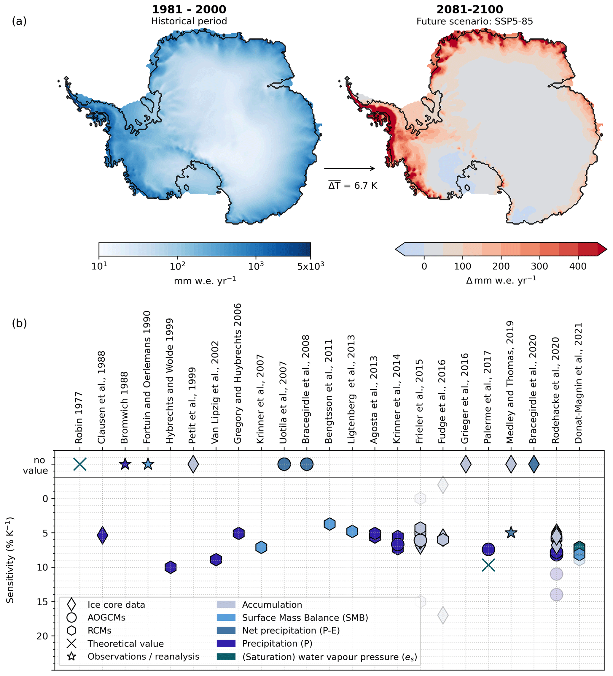
Figure 1 How is Antarctic precipitation changing with warming? (a) Change in mean annual precipitation as simulated with the regional climate model RACMO2.3 (left) for the historical period (1981–2000) and (right) projected for the end of this century (2081–2100) under a high-emission scenario (SSP5-8.5). On average, Antarctica-wide temperatures change by 6.7 K between the two time periods. (b) Literature values from ice core data (diamonds), AOGCMs (atmosphere–ocean general circulation models; circles), and RCMs (regional circulation models; hexagons) as well as observations/reanalysis (stars) for the sensitivity of precipitation, net precipitation, accumulation, and surface mass balance (often linked to the sensitivity of saturation water vapour pressure) to warming (given in % K⁻¹). Upper row shows studies assessing the relationship but without quantifying such a sensitivity factor. Translucent markers indicate extreme values found for example within ice cores (Fudge et al., 2016) or in modelling results (Frieler et al., 2015; Rodehacke et al., 2020; Donat-Magnin et al., 2021).

Despite the little annual snowfall, mass gains through snowfall have exceeded mass losses from the Antarctic Ice Sheet between 2003 and 2008 (Zwally et al., 2015). Model simulations show that Antarctic snowfall may increase significantly in a warming climate and could thus partly buffer the warming-induced ice loss (Bracegirdle et al., 2008; Frieler et al., 2015; Rodehacke et al., 2020). While insignificant changes in snowfall were reported from 1957 to 2006 (Monaghan et al., 2006), Medley and Thomas (2019) find that snow accumulation had been increasing by 1.1 mm w.e. per decade between 1901 and 2000 and by 2.5 mm w.e. per decade after 1979, mitigating sea-level rise by about 10 mm since 1901.

It can be hypothesised that Antarctic snowfall increases with temperature according to the Clausius–Clapeyron relationship (Clapeyron, 1834; Clausius, 1850), describing the saturation water vapour pressure e_s as a function of temperature T. This hypothesis is based on the assumption that Antarctic precipitation is solely driven by temperature and the associated availability of moisture in the atmosphere. Under this assumption, Antarctic snowfall increases with the same sensitivity as the general capacity of the air to hold moisture, which is given by the saturation water vapour pressure e_s, beyond which water vapour condenses and can thus potentially precipitate as snow in Antarctica. Held and Soden (2006) introduce the Clausius–Clapeyron relationship as

$$\begin{array}{}\text{(1)}& {\displaystyle \frac{\mathrm{d}\ln e_{\mathrm{s}}}{\mathrm{d}T}}={\displaystyle \frac{L}{R_{\mathrm{v}}{T}^{\mathrm{2}}}}\equiv \mathit{\alpha }\left(T\right),\end{array}$$

with L being the latent heat of vaporisation and R_v being the specific gas constant for water vapour. α(T) in Eq. (1) is the sensitivity parameter, translating the change in temperature into a relative change in saturation water vapour pressure. With L = 2.5 × 10⁶ J kg ⁻¹, R_v = 461 J K⁻¹ kg⁻¹, and a mean temperature of the lower troposphere where the moisture resides of about T=260 K (e.g. Hartmann, 2016), the global scaling factor lies at around 8 % K⁻¹. If we were to use the continent-wide Antarctic mean annual surface air temperature of T_g = 239.6 K (−33.6 ^∘C, 1981–2000 mean of ERA5-Land reanalysis data), the sensitivity factor α(T_g) would be calculated as 9.4 % K⁻¹. However, such a calculation using surface air temperatures is biased because changes in the surface temperature T_g are larger than changes in the temperature of the moisture-holding free atmosphere above the prevailing surface inversion layer (Jouzel and Merlivat, 1984; Connolley, 1996). Fortuin and Oerlemans (1990) suggest that the temperature of the free atmosphere above the inversion in Antarctica T_f can be approximated from the surface temperature T_g (in kelvin) as

$$\begin{array}{}\text{(2)}& T_{\mathrm{f}}\left[\mathrm{K}\right]=\mathrm{0.67}\cdot T_g\left[\mathrm{K}\right]+\mathrm{88.9}.\end{array}$$

Using this approximation, the theoretically obtained sensitivity α(T) from Eq. (1) yields 8.7 % K⁻¹, for a surface air temperature of T_g = 239.6 K (1981–2000 mean of ERA5-Land reanalysis data). We will use this bias-corrected value throughout this paper as an estimate of the continent-scale mean sensitivity for a change in today's surface temperature. For the model simulations, we will analyse the sensitivity directly relative to the modelled change in surface temperature, as this temperature (a) is more readily available from observations and the model simulations and (b) has been the standard measure also in previous studies. An additional correction for the temperature of the moisture-holding layer of the atmosphere is not necessary in this case, as the models resolve the vertical temperature changes in their atmospheric thermodynamic schemes.

Projections of regional climate models show a wide range of snowfall changes in the coming decades depending on the model input (Kittel et al., 2021). Simulations of the regional model RACMO2.3, which is often used as input of numerical ice-sheet models (e.g. in Garbe et al., 2020; Seroussi et al., 2020), project that mean annual Antarctic precipitation will increase from approximately 189 mm w.e. yr⁻¹ in 1981–2000 to 289 mm w.e. yr⁻¹ at the end of the century for the SSP5-8.5 (Shared Socioeconomic Pathway) scenario. This corresponds to an increase of +52.43 % for the simulated mean temperature increase of 6.7 K. In these simulations, precipitation increases most in coastal areas but also rises in the interior (right panel of Fig. 1a). We note that the temperature and the precipitation increase in RACMO2.3 can be considered a very high estimate of the expected changes because the climate model CESM2 that is used to provide lateral boundary conditions for RACMO2.3 has an unrealistically high climate sensitivity (Gettelman et al., 2019).

Global coupled climate models participating in the Coupled Model Intercomparison Project Phase 6 (CMIP6) show differently strong responses of Antarctic precipitation to temperature changes in the 21st century, depending both on the underlying future climate scenario and the specific models. To examine the spread across different future climate scenarios, we analyse the expected changes for three Shared Socioeconomic Pathway (SSP) scenarios for characterising future climatic conditions in Antarctica: SSP1-2.6 as a low-emission, SSP2-4.5 as intermediate-, and SSP5-8.5 as high-emission scenario (Riahi et al., 2017). End-of-century (2081–2100) Antarctic surface air temperatures are projected to change relative to present-day conditions (1981–2000) by 1.6 ± 0.8, 2.7 ± 0.9, and 4.7 ± 1.4 K for the low- (SSP1-2.6), intermediate- (SSP2-4.5), and high-emission scenarios (SSP5-8.5), respectively. For each of these temperature changes, annual precipitation is projected to increase by 9.7 ± 7.3 %, 15.8 ± 8.1 %, and 28.8 ± 12.6 %.

Because it is numerically expensive and technically challenging to couple global atmosphere–ocean general circulation models to an interactive ice sheet, standalone ice-sheet models are usually used that often employ a scaling approach to translate changes in air temperature to changes in Antarctic precipitation. In ice-sheet models, precipitation can be scaled with temperature or temperature anomalies, using sensitivity factors (% K⁻¹) given by the existing literature. This approach is often used in long-term projections, where regional climate model estimates are not available: Albrecht et al. (2020) for instance used different values for the sensitivity factor to perform glacial-cycle simulations and to test for parameter sensitivity. Quiquet et al. (2018) scale the surface mass balance with a sensitivity factor, assessing Antarctic Ice Sheet changes for the last 400 kyr. Huybrechts (2002) deduces the precipitation and basal melt rate from simple temperature relationships for performing glacial-cycle simulations. Rodehacke et al. (2020) scale precipitation with temperatures, estimating Antarctica's sea-level contribution when using different precipitation parameterisations such as CMIP5 model output or constant scaling factors inside the ice-sheet model.

Generally, snowfall in Antarctica depends on a complex interplay of processes. Not only moisture availability and temperature but also the local wind regime (Grazioli et al., 2017), the occurrence of atmospheric rivers, and large-scale atmospheric variability (Nicolas et al., 2017; Wille et al., 2019; Eayrs et al., 2021; Maclennan et al., 2022) play a crucial role. Also the detailed vertical temperature structure of the atmosphere, the density profile of the air and the resulting katabatic winds, the distance from the coast, the surface slope, and the surface shape are of relevance (Fortuin and Oerlemans, 1990). In addition, synoptic-scale features, such as cyclones and fronts, generally influence coastal precipitation (Bromwich, 1988). The large-scale, integrated, long-term evolution of precipitation is, however, found to be generally dominated by thermodynamic changes (Uotila et al., 2007; Krinner et al., 2014; Grieger et al., 2016).

It is known that the Antarctic Ice Sheet may gain mass under warming due to increased snowfall. Such an increase is expected to generally follow a given rise in temperature according to the Clausius–Clapeyron relationship. Already Robin (1977) has proposed a linear relationship between water vapour pressure over ice and temperature, whilst concluding that this is “an empirical approximation to observations, rather than a natural law”. Two of the earliest studies performing regression analyses with accumulation data were Muszynski and Birchfield (1985) and Fortuin and Oerlemans (1990), with the latter study analysing, among other things, analytically how atmospheric stratification and the surface topography impact moisture availability and thus regional precipitation. Krinner et al. (2007), Bengtsson et al. (2011), Ligtenberg et al. (2013), and Agosta et al. (2013) use changes in surface mass balance (SMB) to estimate sensitivity factors between precipitation and temperature, while Frieler et al. (2015), Fudge et al. (2016), and Medley and Thomas (2019) use changes in snow accumulation to derive relative changes in snowfall per degree of warming (% K⁻¹). Other studies have determined a sensitivity of net precipitation to warming, meaning precipitation minus evaporation (commonly denoted P−E), to also account for an increase in evaporation rates (Uotila et al., 2007; Bracegirdle et al., 2008). Palerme et al. (2017) use changes in total precipitation (P) estimates, focusing on the increase in snowfall (+ rain) with warming. Several more studies have analysed a potential connection of mass gains and atmospheric warming (see Fig. 1) but have not estimated a sensitivity factor in the form that is discussed here (% K⁻¹). As data sources for estimating the sensitivity of precipitation, existing studies have incorporated ice core data (Petit et al., 1999; Van Ommen et al., 2004; Frieler et al., 2015; Fudge et al., 2016), ice core data combined with reanalysis (Medley and Thomas, 2019), AOGCM output partaking in early CMIP initiatives (Uotila et al., 2007; Bracegirdle et al., 2008), CMIP3 (Gregory and Huybrechts, 2006; Krinner et al., 2014), and CMIP5 (Frieler et al., 2015; Grieger et al., 2016; Palerme et al., 2017; Rodehacke et al., 2020) or high-resolution, regional, or palaeoclimate model output (Krinner et al., 2007, 2014; Agosta et al., 2013; Ligtenberg et al., 2013; Frieler et al., 2015; Donat-Magnin et al., 2021). Overall, the sensitivity factors assessed from the literature vary roughly between 4 % K⁻¹ and 10 % K⁻¹ (see Fig. 1) with extreme values for the change in snow accumulation found in parts of ice cores (Fudge et al., 2016) and certain modelling studies (Frieler et al., 2015; Donat-Magnin et al., 2021).

In this paper, we update previous continent-wide estimates of the sensitivity factors of Antarctic precipitation to temperature based on the latest available model data and reconcile it with previous approaches (Sect. 3). We show how and explain why these sensitivity factors differ strongly across the ice sheet (Sect. 4). We conclude that the scaling approach often used in ice-sheet models should be revised, depending on the chosen application.

2 Methods

In our study we revisit the temperature dependency of snowfall changes on the Antarctic Ice Sheet. We use a least-squares regression analysis to determine the sensitivity factor α that describes how Antarctic precipitation changes with temperature. This approach follows the general definition of the Clausius–Clapeyron relationship (Eq. 1). Sensitivity factors have been commonly estimated using relative changes in precipitation or accumulation (changes in percent compared to a reference period) and values of warming (ΔT; e.g. Frieler et al., 2015; Fudge et al., 2016; Palerme et al., 2017). For example, Frieler et al. (2015) use changes in warming and relative changes in precipitation compared to 1850–1900. Krinner et al. (2007, 2014) and Palerme et al. (2017) compare changes between two states, e.g. the end of the 20th century versus the end of the 21st century.

In our analysis, we follow the Clausius–Clapeyron theory (Eq. 1) more closely, applying the regression analysis to log-scaled mean annual precipitation and the annual temperature time series. This makes our approach independent of the chosen reference period. Donat-Magnin et al. (2021) use a similar approach, but they do not account for the full length of the available time series. As discussed above, for the model simulations we analyse sensitivities only as a function of mean annual surface air temperatures, as the models implicitly resolve the impact of the vertically varying temperature profile in their calculation of precipitation.

We perform a sensitivity analysis in the following three ways.

1. Continent-wide temporal regression. We first average over available temperature and precipitation fields (weighted by surface area) across the entire Antarctic continent and then obtain a sensitivity value from the least-squares regression of the time series of continent-wide annual temperature and log-scaled precipitation. To compare our results to previous studies, we repeat a temporal regression using precipitation anomalies relative to a reference period (linear regression).

2. Grid-point temporal regression. We first perform the least-squares regression with the local time series of annual temperature and log-scaled precipitation for every grid point. In this regression the predictor arrays are the time series of temperature for each grid point, respectively. This yields a spatial distribution of scaling factors. For comparing these estimates to the continent-wide temporal regression, these grid values are averaged over the ice sheet (area-weighted).

3. Spatial regression. For each time slice of the available data (x,y, time), we perform a least-squares regression with the data points from the spatial distribution of temperature and log-scaled precipitation (x,y). Here the predictor values are the 1440 × 1080 (longitude × latitude) grid points of temperature values for each time slice. The regression with the 1440 × 1080 grid points of precipitation then yields a new estimate of the sensitivity of how Antarctic precipitation follows local temperatures across the ice sheet. For analysing the change in this sensitivity with temperature, we perform a temporal regression of the scaling factors with the mean annual temperature time series. This second step makes this approach distinct from the grid-point regression where only a temporal regression is performed.

Our analysis is based on different types of data to robustly delineate the sensitivity of Antarctic precipitation to temperature under present-day conditions, as well as their potential changes in the future.

While direct measurements are scarce and observational products such as the CloudSat data lack the needed resolution (Palerme et al., 2014), we use the ECMWF ERA5-Land reanalysis data (Muñoz Sabater, 2019) as a best estimate of present-day conditions in Antarctica. These reanalysis data provide spatially and temporally complete coverage of the historical and present-day evolution of precipitation and temperature patterns for Antarctica. The ERA5-Land reanalysis is provided through the Copernicus Climate Change Service (C3S) at the Climate Data Store and is available at a resolution of 0.1^∘ × 0.1^∘ on a longitude–latitude grid at hourly resolution. We here use monthly averaged variables.

In addition, we analyse CMIP6 model data which are available from the Earth System Grid Federation (ESGF; for example at https://esgf-data.dkrz.de, last access: 10 July 2022). We combine historical data that cover the period of 1850–2014 with projections for the years 2015 to 2100. A few models provide projections until the year 2300, including for the low-emission SSP1-2.6 scenario models CanESM5, IPSL-CM6A-LR, MRI-ESM2-0, and UKESM1-0-LL, and additionally for the high-emission SSP5-8.5 scenario models ACCESS-CM2 and MIROC-ES2L. We use the first available ensemble member of each CMIP6 model for analysis. The nominal resolution of the CMIP6 ensemble differs substantially and lies between 50 km (CNRM-CM6-1-HR and GFDL-CM4) and 500 km (CanESM5). If possible we use the native model mask (through the variable “sftlf”) to extract data for the Antarctic continent. For analysing the regional CMIP6 model mean of sensitivity factors, we regrid all models to a common 1440 × 1080 grid, following the highest resolution of the available models (GFDL CM4). We incorporate more than 30 different models for the analysis until 2100.

Adding to that, we use mean monthly values of near-surface temperature and precipitation data from the regional model RACMO2.3 for the years 1950 to the end of the 21st century (van Meijgaard et al., 2008; Van Wessem et al., 2018). For the future period 2015–2100, RACMO2.3 is here forced with CESM2 model output for the SSP5-8.5 scenario, which, as discussed above, might have given rise to too high estimates of future warming. The data are available at a 27 km resolution.

We analyse the full time series of yearly mean temperature and precipitation until the year 2100 (and in some cases until 2300). In order to obtain a reference period for the 20th century and the 21st century, we average values over the years 1981–2000 and 2081–2100, respectively. We use a 20-year average to reduce the impact of internal variability, following the approach in the recent IPCC AR6 WGI (Intergovernmental Panel on Climate Change Sixth Assessment Report Working Group I) report (Masson-Delmotte et al., 2021). Mean values of both time windows will be used to assess sensitivity factors as in Palerme et al. (2017).

3 Continent-wide scaling factors from data of regional and global climate models

Analysing Antarctic temperature and precipitation from all available CMIP6 models over the time period 1850–2100, we find a sensitivity of Antarctic precipitation to temperature of approx. α = 5.5 % K⁻¹, which is independent of the chosen climate-change scenario and close to previous estimates. The statistical means across all individual CMIP6 sensitivities from the continent-wide temporal regression are 5.5 ± 1.2 % K⁻¹, 5.5 ± 1.1 % K⁻¹, and 5.5 ± 0.9 % K⁻¹ using the historical period and the three SSP scenarios, respectively (SSP1-2.6, SSP2-4.5, SSP5-8.5). Using the inter-model mean of Antarctic precipitation and temperature results in slightly higher values of α = 6.2 % K⁻¹, 5.9 % K⁻¹ and 5.7 % K⁻¹ (see Fig. 2). RACMO2.3 data give a sensitivity factor of α = 6.4 % K⁻¹ using the SSP5-8.5 scenario with the available historical period from 1950 to 2100; 6.4 % K⁻¹ lies close to the upper end of the inter-model spread of the CMIP6 ensemble for the SSP5-8.5 scenario (5.5 ± 0.9 % K⁻¹), and the deviation could thus generally be explained by differing model climate sensitivities.

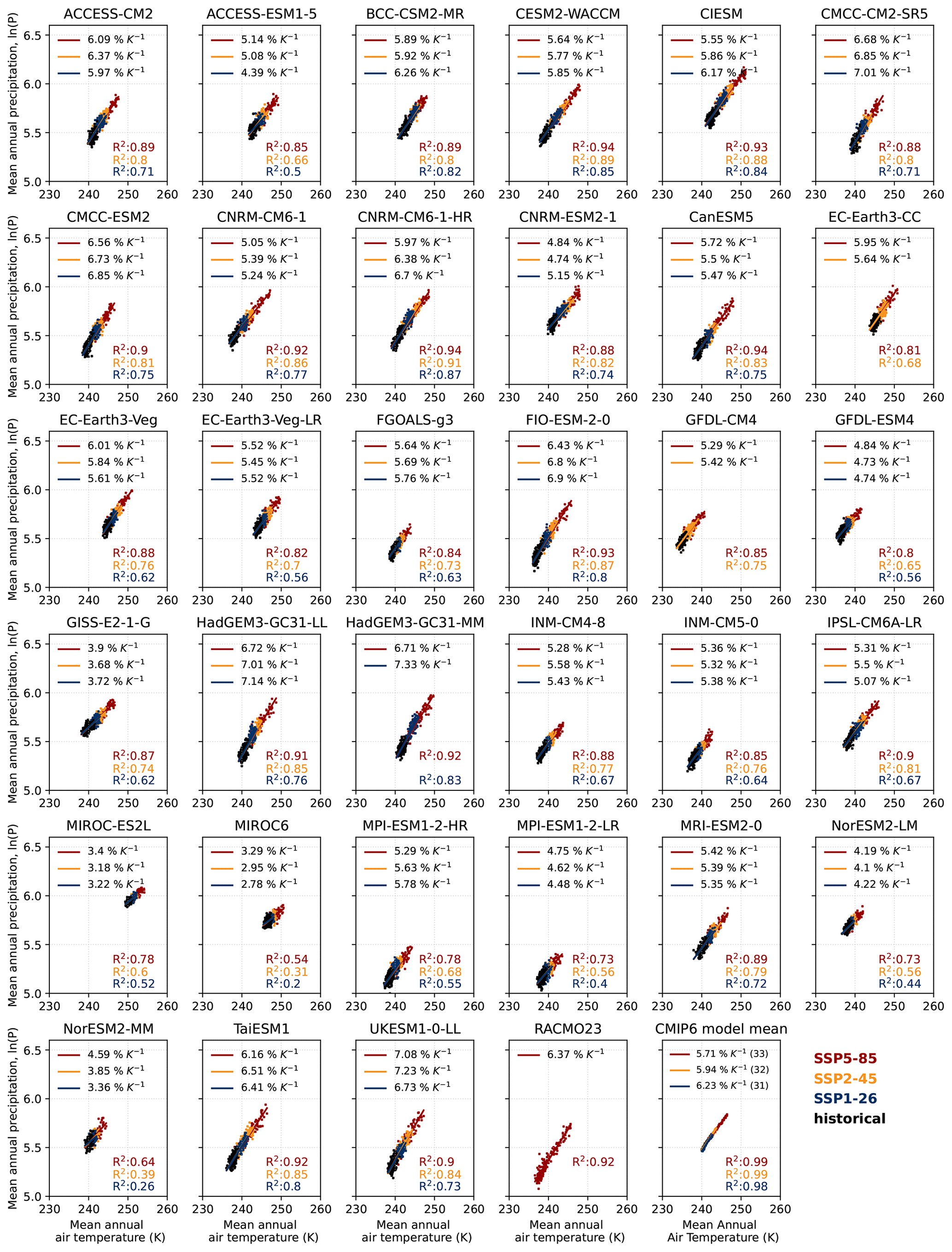
Figure 2 Update on continent-wide scaling factors based on CMIP6 and RACMO2.3 projections for the 21st century. Sensitivity factors are estimated over the period 1850–2100 for the CMIP6 ensemble by combining the historical period with three available Shared Socioeconomic Pathway scenarios (SSP1-2.6, SSP2-4.5, and SSP5-8.5) and over the period 1950–2100 for RACMO2.3. For the CMIP6 model mean, the numbers in brackets refer to the number of models incorporated into the analysis.

The R² values of the performed temporal regressions with the CMIP6 model data are generally highest for the SSP5-8.5 scenario with R² up to 0.94 for models CESM2-WACCM, CNRM-CM6-1-HR, and CanESM5 (see Fig. 2 for details). These high values of R² in the high-emission scenario arise probably from the high signal-to-noise ratio that is obtained through the high warming rates in SSP5-8.5. Note that at the time of our analyses not all CMIP6 models provided all future scenarios. All model-specific scaling factors are summarised in Table A1 in the Appendix. For the RACMO2.3 data we obtain an R² value of 0.92.

Our sensitivity factor of approx. 5.5 % K⁻¹ as the average across CMIP6 models is slightly lower than the CMIP5 estimate of 6.1 % K⁻¹ derived in Frieler et al. (2015). This can in part result from differences in the CMIP6 versus the CMIP5 ensemble (Zelinka et al., 2020; Payne et al., 2021). Moreover, as described above we are using a log-based approach here rather than relative anomalies, which also leads to slightly different estimates. Using the same approach as in Frieler et al. (2015) (i.e. anomalies with respect to 1890–1980), we obtain a mean sensitivity of 5.9 ± 1.3 % K⁻¹. Individual model results from this analysis are shown in Appendix Fig. A2. Quantifying the changes between the two reference periods, i.e. the end of the 20th versus the end of the 21st century, results in a higher sensitivity of 7.3 % K⁻¹ (see Fig. A3), which is close to the CMIP5 estimate in Palerme et al. (2017). This shows that the calculated sensitivity depends on the chosen analysis method.

For the extended CMIP6 projections until 2300, we use the model output by ACCESS-CM2, CanESM5, IPSL-CM6A-LR, MIROC-ES2L, MRI-ESM2-0, and UKESM1-0-LL. For these models we find sensitivities between 4.1 % K⁻¹ and 6.5 % K⁻¹ dependent on the model and the chosen scenario (see Fig. 3). We find that the old approach of estimating sensitivity factors from changes relative to a reference period shows a stronger bias for the SSP5-8.5 scenario (compare Appendix Fig. A2). The sensitivity factors for e.g. the CanESM5 model results in 13.3 % K⁻¹ for a linear temporal regression compared to 6.3 % K⁻¹ in our logarithmic approach. The difference is due to the nature of the regression itself. With a simple linear regression using anomalies, we approximate the exponential function with percentage changes, which only holds for very small changes in the predictor variable, here increments of warming (ΔT). If the chosen model shows strong warming, hence large ΔT, the regression becomes inaccurate. Using output from climate models that show strong warming rates, i.e. that have a high equilibrium climate sensitivity, such as CanESM5 (Meehl et al., 2020), the relative anomaly approach thus significantly alters the results from the multi-model analysis. Our logarithmic approach on the other hand incorporates the exponential function directly in the regression analysis; this avoids a potential bias towards the models with higher climate sensitivity (sometimes referred to as the “hot-model problem”; see e.g. Hausfather et al., 2022).

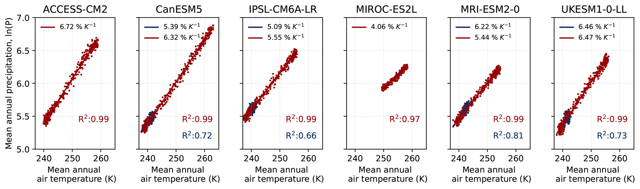
Figure 3 Continent-wide scaling factors for CMIP6 models simulating Antarctic climate change until 2300. Red colours refer to Shared Socioeconomic Pathway SSP5-8.5; blue colours refer to Shared Socioeconomic Pathway SSP1-2.6.

4 Regional sensitivity factors differ across the ice sheet

Performing the grid-point temporal regression of available CMIP6 model data shows that, across the ice sheet, sensitivity factors in certain regions are substantially different from the continental scaling factor of approximately 5.5 % K⁻¹ obtained in the previous section (see Fig. 4). This largely confirms findings by Rodehacke et al. (2020), showing that regional sensitivities can differ substantially from the continent-wide scaling also in CMIP5. Note that we here use the time period of 1950–2100 to compare the spatial sensitivities with the results from RACMO2.3 (which are available for the same time period). Using the period from 1850 to 2100 only causes very minor differences in our results.

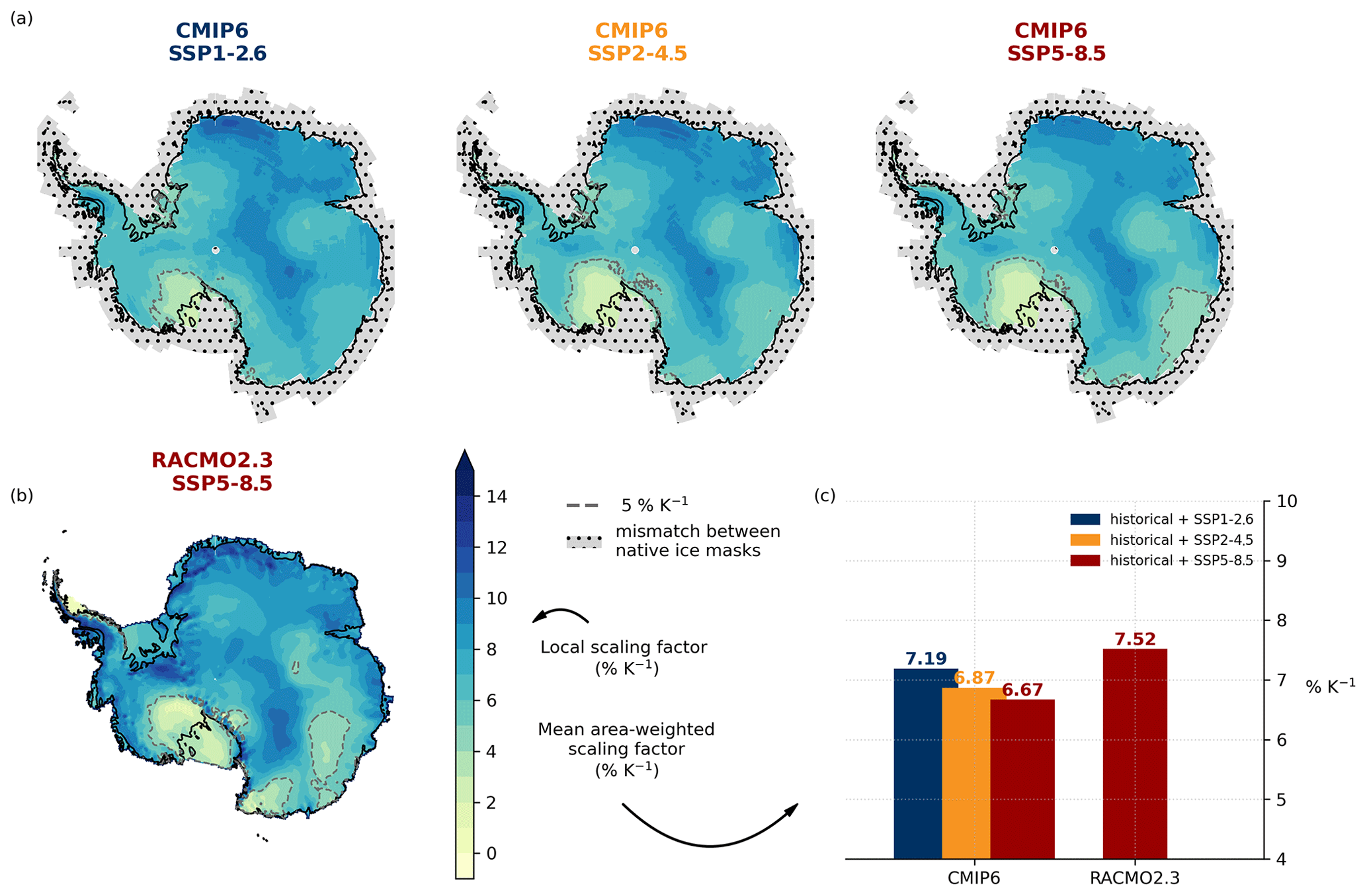
Figure 4 Sensitivity factors across the ice sheet derived from projections for the 21st century. (a) Spatially resolved sensitivities for the CMIP6 model mean for each SSP scenario. The point-wise temporal regression is based on the period 1950 to 2100 by combining the historical period with the SSP1-2.6, SSP2-4.5, and SSP5-8.5 future scenarios, respectively. (b) Spatially resolved sensitivities for RACMO2.3 model data, which were forced by CESM2 with SSP5-8.5 forcing (1950–2100). Dashed lines in maps indicate the 5 % K⁻¹ contour line, which refers to a commonly used sensitivity factor in ice-sheet modelling, such as in Garbe et al. (2020). Hatched regions show a mismatch between native ice masks of the CMIP6 ensemble, which are excluded from the analysis. (c) Comparison of area-weighted mean sensitivities, averaged over the same area of interpolated CMIP6 and RACMO2.3 data.

The spatial sensitivities obtained from the multi-model mean of the regridded temperature and precipitation fields show similar patterns across the different SSP scenarios: in the Ross Ice Shelf region there are very low sensitivity factors, while in the interior factors go up to more than 10 % K⁻¹. Sensitivity factors are on average around 2 % higher in East Antarctica than in West Antarctica (here given roughly by the 40^∘ W/320^∘ E and 180^∘ W/180^∘ E longitudes as lateral boundaries). We here acknowledge more sophisticated ice-dynamics-based definitions, i.e. that are derived from ice divides of individual ice drainage basins (Rignot et al., 2011; Zwally et al., 2012). For the three chosen SSP scenarios, the mean area-weighted factors are 7.7 % K⁻¹, 7.4 % K⁻¹, and 7.2 % K⁻¹ for East Antarctica and 5.7 % K⁻¹, 5.4 % K⁻¹, and 5.3 % K⁻¹ for the West Antarctic Ice Sheet, respectively. The mean R² values for the East Antarctic Ice Sheet (EAIS) are higher than for the West Antarctic Ice Sheet (WAIS) (R² = 0.79, 0.86, and 0.94 versus R² = 0.64, 0.72, and 0.85 for the respective future scenarios; compare Appendix Fig. A4). The difference between the two ice sheets could result from the low sensitivity factors found near Siple Coast, where the temporal regression performs very poorly and skews the mean for the WAIS to lower values. This could be for instance due to a prominent area of converging katabatic winds (Parish and Bromwich, 2007), which could diminish precipitation at the coast (Grazioli et al., 2017), or generally hints at the large imprint of dynamic atmospheric systems in the area.

Comparing sensitivity factors across the ice sheet with the respective present-day temperatures (see Appendix Fig. A1) allows us to explain much of the spatial patterns: higher sensitivity factors are generally found in regions with lower temperatures. This is consistent with the theory, as the Clausius–Clapeyron relationship in Eq. (1) gives higher values of α for colder temperatures. Local temperatures especially in East Antarctica can reach well below the mean annual air temperature of 239.6 K/−33.6 ^∘C (1980–2000 mean from the ERA5-Land reanalysis). This temperature results in a theoretical sensitivity factor of 8.7 % K⁻¹ when correcting for the slower warming of the atmosphere compared to the surface (see above). This estimate is consistent with the sensitivity factors we find in the cold Antarctic interior (see Fig. 4). In general, the relationship between local temperatures and sensitivity factors is most pronounced on the East Antarctic plateau, where the influence of coastal winds is considered to be less significant (Bromwich, 1988). The effect of a more continental climate is supported by ice core studies from Law Dome and Taylor Dome in East Antarctica: Van Ommen et al. (2004) show that during the Last Glacial Maximum, the local climate was closer to present-day central Antarctica as glacial accumulation rates were more closely tied to saturation vapour pressure than in the Holocene.

While the overall spatial pattern is robust for the different climate-change scenarios, the sensitivity factors are generally lower for the high-emission SSP5-8.5 scenario and higher for the low-emission SSP1-2.6 scenario. This tendency can be seen in the local factors across the ice sheet, with the difference between scenarios being particularly pronounced in East Antarctica. The tendency of lower sensitivity factors for higher emissions is even more apparent when averaging over the scaling factors for each scenario (see Fig. 4c): we find a mean area-weighted scaling factor of 7.2 % K⁻¹, 6.9 % K⁻¹, and 6.7 % K⁻¹ for the SSP1-2.6, SSP2-4.5, and SSP5-8.5 scenario, respectively. This is consistent with the RACMO2.3 mean scaling factor of 7.5 % K⁻¹ for the SSP5-8.5 scenario.

This mean of the spatially resolved sensitivity factors of the CMIP6 model data is thus higher than the continent-wide estimate of 5.5 % K⁻¹, which was independent of the chosen warming scenario (note the difference between the mean of the grid-point scaling factors and the continent-wide scaling factor; see “Methods”). This difference in sensitivity factors is due to the non-linearity (logarithmic relationship). Local differences are diminished when generating the continent-wide temperature and annual precipitation time series. For the RACMO2.3 model we find small regions of high sensitivity factors in parts of Dronning Maud Land and around the Filchner–Ronne Ice Shelf that are not visible in the CMIP6 model results (see Fig. 4). We believe this is due to local dynamic effects which are incorporated in the regional climate models and are not resolved in the CMIP6 models. This is consisted with regional studies, finding scaling factors of 7.4 % K⁻¹ to 8.9 % K⁻¹ for the Amundsen Sea region (Donat-Magnin et al., 2021).

We find an even stronger difference between a “cold” and a “warm” future scenario when examining the local sensitivity factors from those models that simulate Antarctic precipitation and temperature until 2300 (see Fig. 5). The results of the low- (SSP1-2.6) and high-emission (SSP5-8.5) scenario show a strong difference in temperature sensitivities across the ice sheet. For the SSP1-2.6 scenario, the area-weighted mean scaling factors across the ice sheet are > 8 % K⁻¹. For the warmer SSP5-8.5 scenario, we find much lower sensitivities. The differences in the area-weighted mean scaling factors between the two scenarios lie between 0.9 % K⁻¹ for CanESM5 and 2.9 % K⁻¹ for the MRI-ESM2-0 model. Here the CanESM5 model shows local warming of > 30 K by 2300 compared to the present day, which leads to a strong reduction in sensitivity as expected from the definition of α.

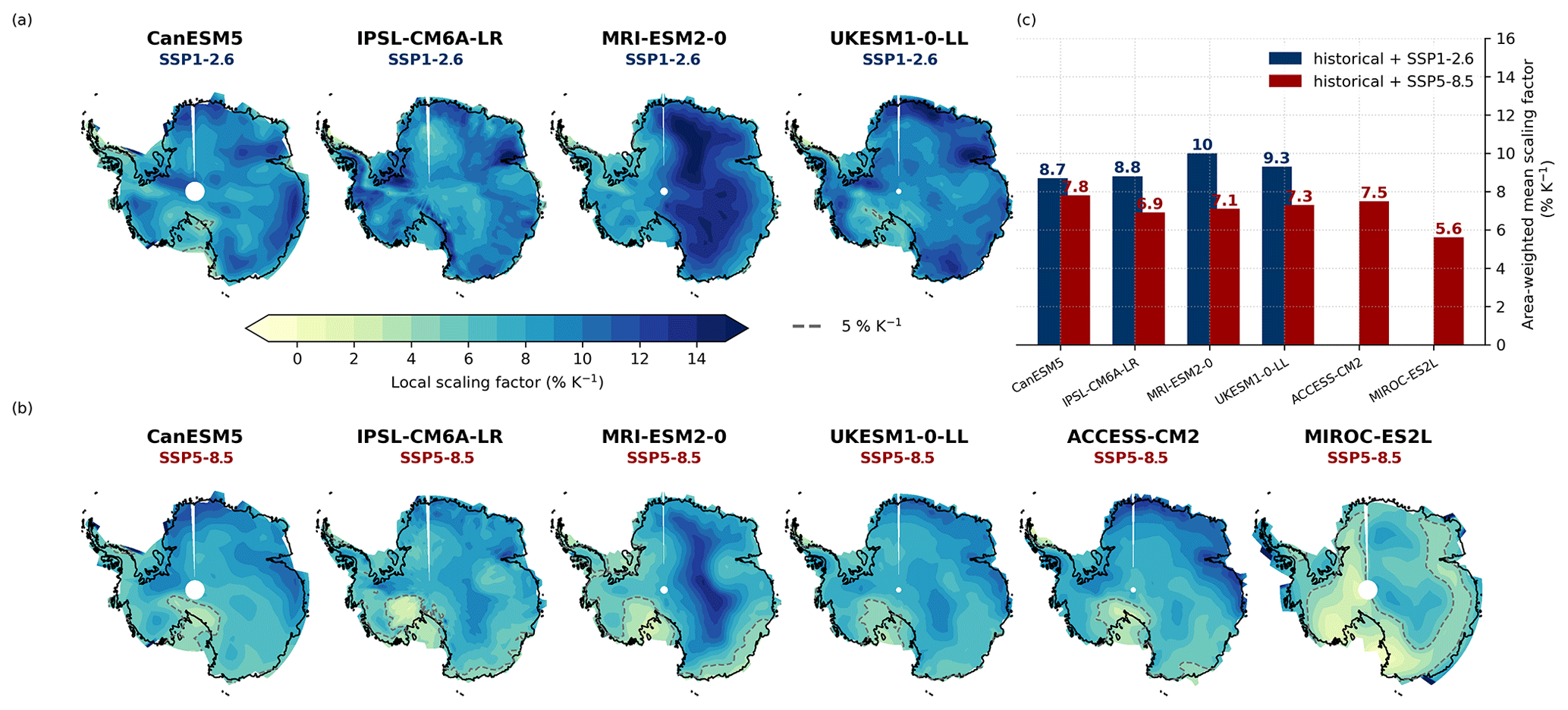
Figure 5 Sensitivity factors across the ice sheet derived from projections until 2300. Results are given for individual CMIP6 models that were run until the year 2300 for (a) SSP1-2.6 and (b) SSP5-8.5. Dashed lines in maps indicate the 5 % K⁻¹ contour line, which refers to a commonly used sensitivity factor in ice-sheet modelling, such as in Garbe et al. (2020). (c) Comparison of area-weighted mean sensitivities.

Our results highlight that when simulating changes in Antarctic mass balance in the future, we need to consider these local sensitivities of precipitation change to warming. Using spatially resolved scaling factors that depict the local conditions could improve projections of the Antarctic sea-level contribution.

As we find that local sensitivity factors depend on the warming level, ice-sheet models which base their precipitation projections on parameterisations derived from these sensitivity factors might overestimate warming-induced snowfall changes, particularly in high-emission scenarios.

5 Discussion and conclusion

The Clausius–Clapeyron equation suggests a clear relationship between changes in temperature and in the moisture-holding capacity of the air, which can potentially be translated into a relationship between changes in temperature and precipitation. Our study amends the existing literature by analysing the regional and continent-wide scaling factors obtained from the latest available model data from regional model RACMO2.3 and the CMIP6 model ensemble.

Overall, we find that the suite of formerly applied methods to establish the sensitivity of potential precipitation changes in Antarctic for a given amount of warming yields different results. Especially when analysing high-end scenarios with strong changes in annual air temperatures, multi-model mean values can be skewed if the sensitivity factors are calculated through relative changes to a fixed reference period. When using a logarithmic approach for the temporal regression analysis, we generally obtain more robust results because the Clausius–Clapeyron relationship is logarithmic by nature.

Across all considered SSP scenarios for the period 1850–2100, local scaling factors obtained through grid-point-wise temporal regression can exceed 10 % K⁻¹, while continent-wide scaling factors from annual mean temperatures and precipitation only yield approximately 5.5 % K⁻¹ for all scenarios. This value lies substantially below the theoretical value of 8.7 % K⁻¹ for the reference period for the 20th century (see above). This discrepancy highlights the necessity to use spatially resolved sensitivity factors when scaling local precipitation patterns into the future.

Moreover, Van Ommen et al. (2004) and Fudge et al. (2016) find a temporally varying relationship between temperature and accumulation rate in ice core data. Assuming one constant scaling factor may hence not capture an evolving scaling relationship through space and time.

While the change in precipitation in the interior of the Antarctic continent follows the theory quite closely, the scaling factors near the coast can be substantially lower. This can be explained by the presence of a pronounced coastal wind regime that substantially affects local precipitation (Grazioli et al., 2017; Lemonnier et al., 2019).

This becomes evident when performing a spatial regression with present-day temperature and precipitation fields. When analysing to which degree the regional temperature distribution can explain the regional distribution of precipitation rates across the ice sheet, we find that the temperature pattern in Antarctica can explain roughly 83 % of the annual precipitation when assuming a direct relationship between the temperature and precipitation fields. This estimate is similar to the value of 72 % explained variance calculated by Fortuin and Oerlemans (1990) for the interior of the ice sheet. Similarly to their study, we find that the estimate of the local precipitation rate based on a simple spatial regression with temperature agrees particularly well with observations in the East Antarctic plateau above 3000 m altitude (see Fig. 6b). In contrast, large differences between estimated and observed precipitation are prevalent in particular in the coastal regions.

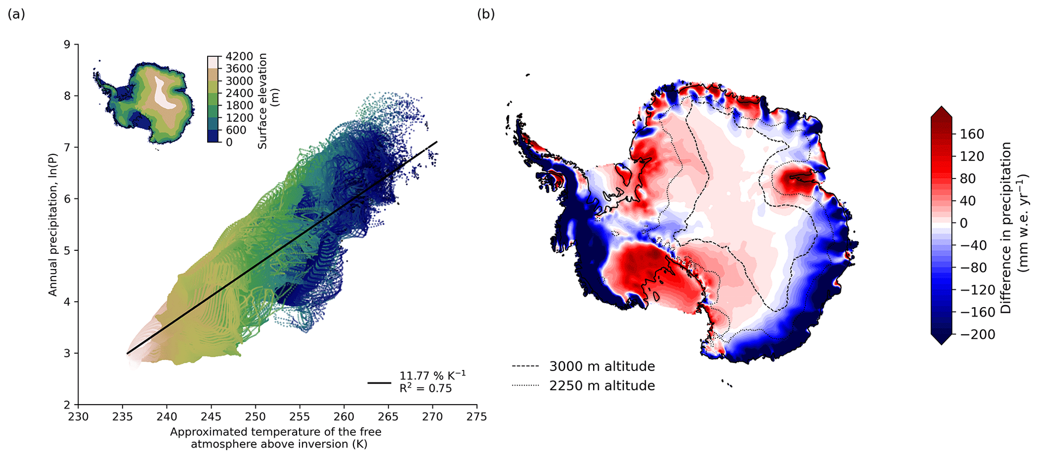
Figure 6 Antarctic precipitation determined by temperatures across the ice sheet. (a) Estimates of log-scaled precipitation against the temperature of the free atmosphere above the inversion, which is deduced from mean annual surface air temperatures for each grid point in the ERA5-Land reanalysis (1981–2000 mean), using Eq. (2). (b) When assuming the simple spatial regression derived from panel (a) between precipitation and temperatures, reanalysed coastal precipitation is mostly underestimated (blue areas), while precipitation around Ross Ice Shelf is largely overestimated (red areas).

The Southern Ocean system is additionally affected by large-scale variability in atmospheric conditions, for example changing storm tracks or changing pressure systems (Bromwich et al., 2004; Eayrs et al., 2021). Especially in West Antarctica, studies suggest a strong El Niño–Southern Oscillation imprint on precipitation (Garreaud and Battisti, 1999; Bromwich et al., 2004; Nicolas et al., 2017). This underlines the necessity for incorporating ice sheets as coupled components into Earth system models to explicitly be able to calculate the resulting interactions. This is particularly the case for multi-millennial integrations. While e.g. storm surges affect Antarctic precipitation on short timescales and on the regional scale, we expect thermodynamic changes to dominate the integrated changes in precipitation. One could therefore argue that constraining the expected horizontal and vertical distribution of future warming above the Antarctic continent should have the highest priority in model development.

Another factor that affects the robustness of the estimated scaling factors from surface temperature is related to the structure of the atmosphere. As discussed above, when analysing model output, we can directly assess the relationship between surface temperature (or the temperature at any other level if we so wished) and precipitation because the models explicitly calculate the humidity and temperature of any atmospheric layer that carries the moisture. When using the Clausius–Clapeyron equation directly to estimate scaling factors, we need to parameterise the relationship between surface temperature and the temperature of the moisture-holding layer. This is particularly challenging in Antarctica, where the vertical temperature profile does not follow a simple adiabatic (or moist-adiabatic) profile but is instead characterised by a pronounced inversion. The impact of this inversion can be approximated by Eq. (2), which then allows us to estimate the temperature of the moisture-holding layer from surface temperature for a typical inversion profile. As the inversion structure is not constant, some uncertainty is introduced into our estimates of the scaling factor by using this approximation for all our calculations. In addition, we can expect the inversion structure to weaken over time, as increasing CO₂ levels in the atmosphere weakens the radiative cooling in the atmosphere that contributes to the intensification of the temperature inversion with elevation.

Another explanation for the lower sensitivity factors than the theory suggest could be potential evaporation constraints, as suggested for instance by Li et al. (2013). Analysing CMIP5 model data, they find that precipitation increases with temperature globally only between 1.5 % K⁻¹ and 3 % K⁻¹. They conclude that one must take into account the energetic constraints on evaporation (approx. 1 % K⁻¹–4 % K⁻¹ in the range of 0–30 ^∘C) when analysing the precipitation scaling globally. We find however that our results do not differ much when analysing net precipitation (precipitation minus evaporation) versus precipitation as done here.

Following Eq. (1) we could see a slight decrease in sensitivity factors across the ice sheet depending on the chosen warming scenario in Sect. 4. This is also apparent when repeating the spatial regression analysis for each year from 1850 to the end of the 21st century (23rd century, where data are available): we find that the 20-year running mean sensitivity declines by −0.064 (±0.045), −0.060 (±0.036), or −0.065 (±0.039) points per degree of temperature rise in the SSP1-2.6, SSP2-4.5, and SSP5-8.5 scenario, respectively (see Appendix Fig. A5). This decrease in sensitivity over time is especially strong for the simulations extending until the year 2300. The low sensitivity in a warmer climate is consistent with the theory of Clausius–Clapeyron, as in colder conditions; for instance in large parts of East Antarctica, the increase in the moisture-holding capacity with warming should be higher.

For the forcing of ice-sheet models, which typically rely on a fixed parameterisation with a single sensitivity factor for all temperature ranges; we therefore suggest introducing temperature-dependent scaling factors, especially for high-end sea-level rise simulations. How well a new precipitation scaling parameterisation in ice-sheet models performs compared to direct input by regional or global climate models still needs to be further tested. When performing ice-sheet model simulations with this new set of sensitivity factors, it would be recommended to include a thorough discussion on the uncertainties arising from the scaling relationship, especially in the coastal areas.

Whether – and on which timescales – increased snowfall can offset dynamic ice loss from the Antarctic Ice Sheet in the future remains very uncertain. For such an analysis, one must in particular consider the feedback that snowfall has on the general ice dynamics, since it is known that increased snowfall at the ice-sheet margins enhances the ice flow and thus the ice discharge across the grounding line (Winkelmann et al., 2012). Garbe et al. (2020), using exponentially scaled precipitation, show that despite an increase in surface mass balance, large parts of the Antarctic Ice Sheet could disintegrate in the long-term, with a first critical warming threshold at around 2 ^∘C of global warming above pre-industrial levels, where the West Antarctic Ice Sheet might become unstable. This means that ice losses, further accelerated by the marine ice-sheet instability (see e.g. Robel et al., 2019), cannot be compensated by additional snowfall as previously assumed. The assumption that increased snowfall directly translates into an increase in surface mass balance in the future can be further contested by studies investigating the non-linear growth in melt and runoff under warming (Gilbert and Kittel, 2021; van Wessem et al., 2023). Accumulation processes are complex, and with increasing melt of snow and of the subsequent firn layer, increased precipitation does not necessarily lead to a mass gain in all parts of Antarctica. Given the present-day temperature conditions, most precipitation falls as snow in Antarctica. With ongoing warming, however, rainfall will likely increase in amount, frequency, and intensity along the coast of Antarctica over the next 80 years (Vignon et al., 2021). If more precipitation falls as liquid rain, the remaining water on the ice-sheet surface may amplify ongoing surface melt processes through the reduction in surface albedo, latent heat release, or hydro-fracturing (Kopp et al., 2017).

For future projections, it will remain important to approximate precipitation increases through temperature-scaling approaches, as coupled simulations with regional climate models remain computationally expensive, especially on multi-centennial timescales. Our results show that these scaling approaches can in principle capture the overall changes in precipitation in a warming world sufficiently well; however, when using a precipitation-scaling approach in ice-sheet modelling studies, the scaling parameter needs to be chosen according to the given application, and its choice should potentially reflect the more complex temperature dependency outlined here. In particular, our results suggest that Antarctic mass balance projections with uniform estimates of the scaling factor might overestimate the compensating effect of additional snowfall under future warming.

Appendix A: Additional figures to the sensitivity analysis

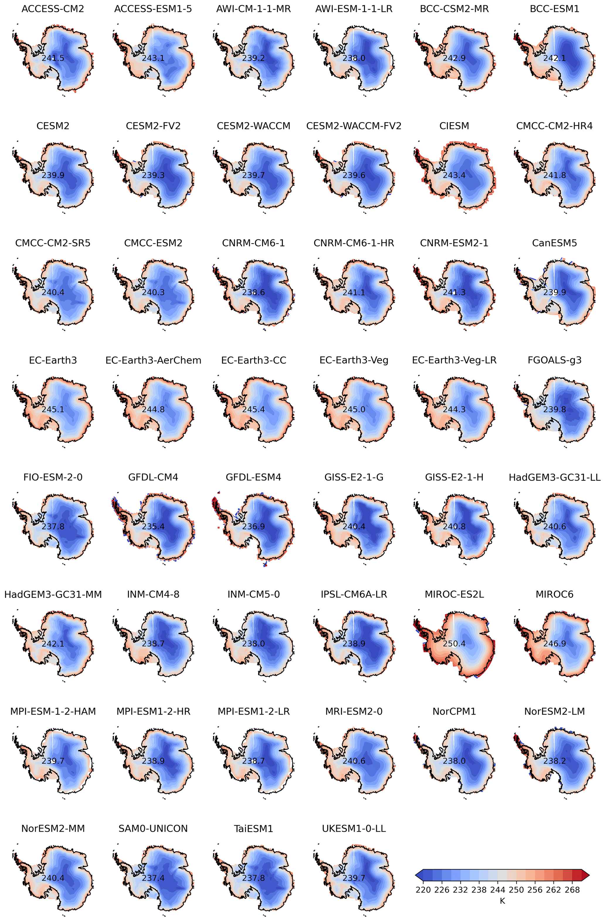
Figure A1 Mean annual air temperature for present-day conditions (1981–2000) from the CMIP6 model ensemble.

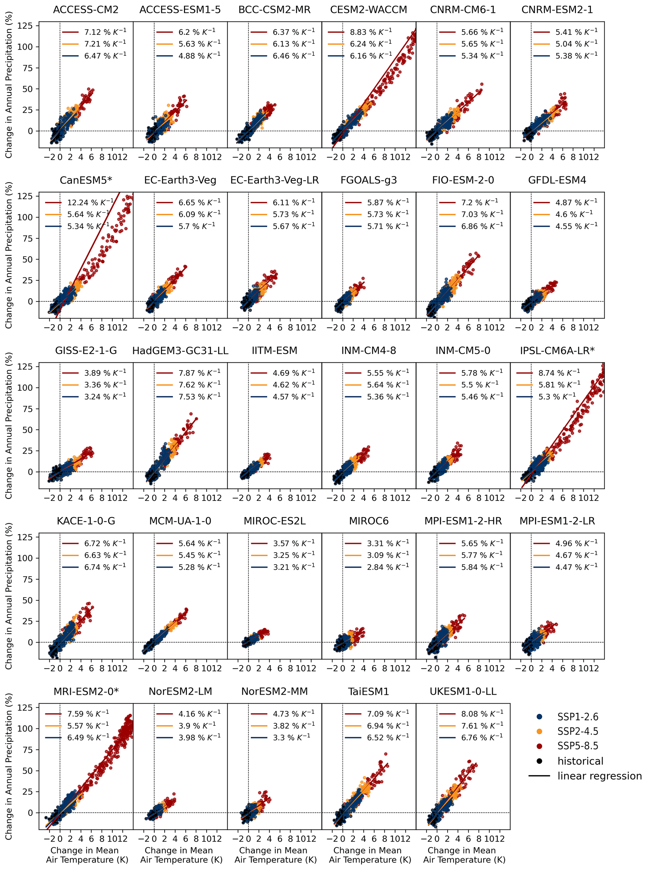
Figure A2 Models indicated with an asterisk (*) simulate Antarctic climate change up to the year 2300. For the temporal regression analysis the full available time series were used.

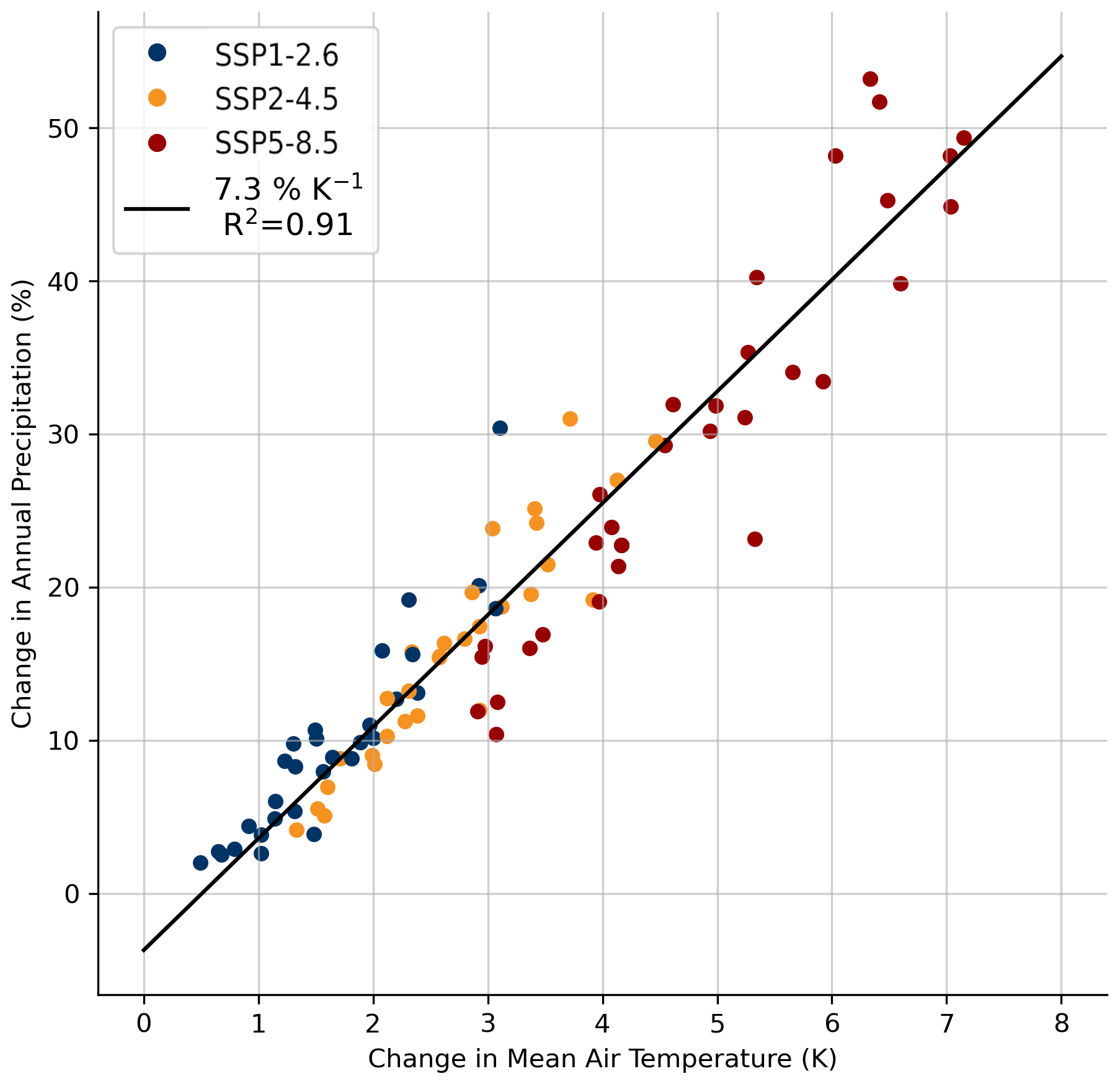
Figure A3 Each dot represents an individual model result on how much Antarctic precipitation and temperature have changed between the end of the 20th century (1981–2000) and the end of the 21st century (2081–2100).

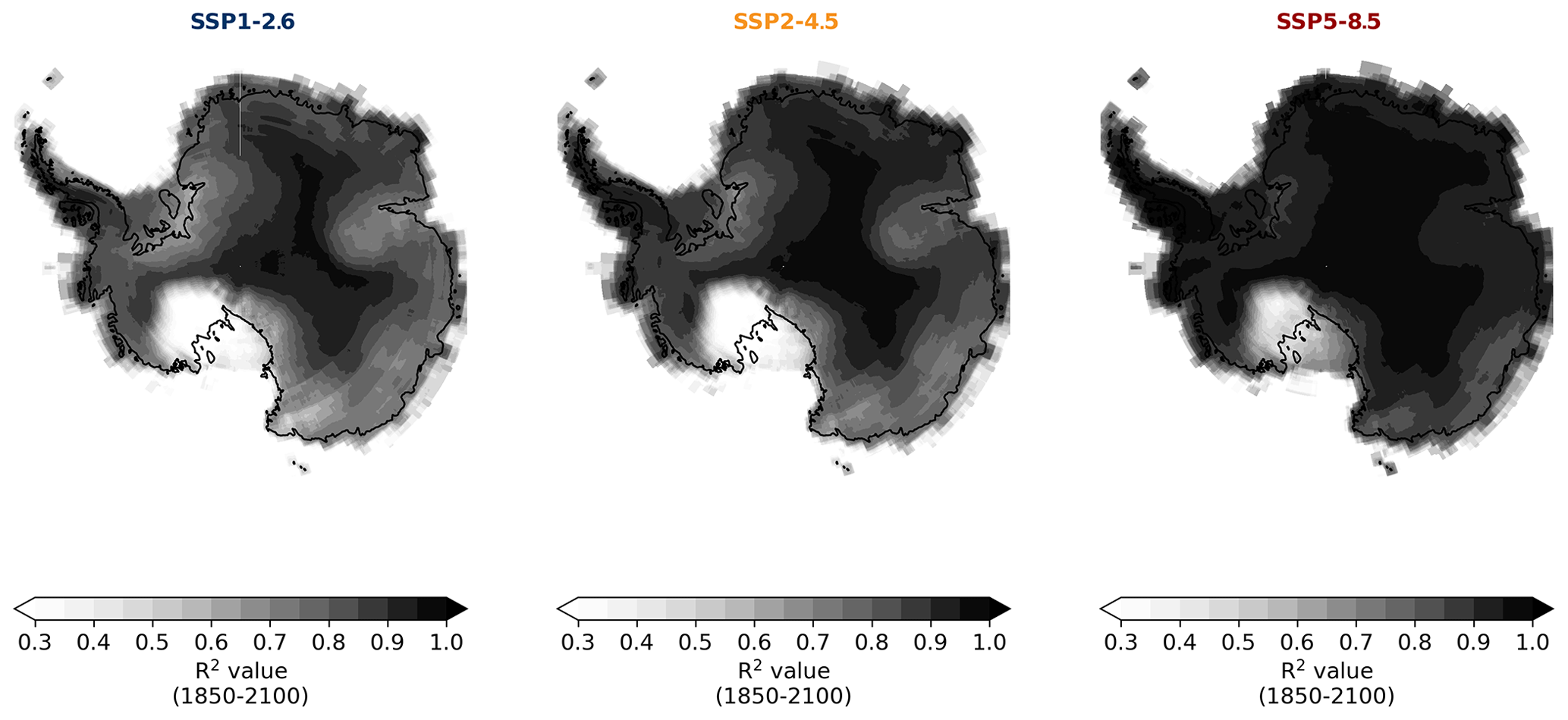
Figure A4 R² values of performed grid-point-wise temporal regression using the CMIP6 ensemble mean of the different SSP scenarios SSP1-2.6, SSP2-4.5, and SSP5-8.5 (1950–2100).

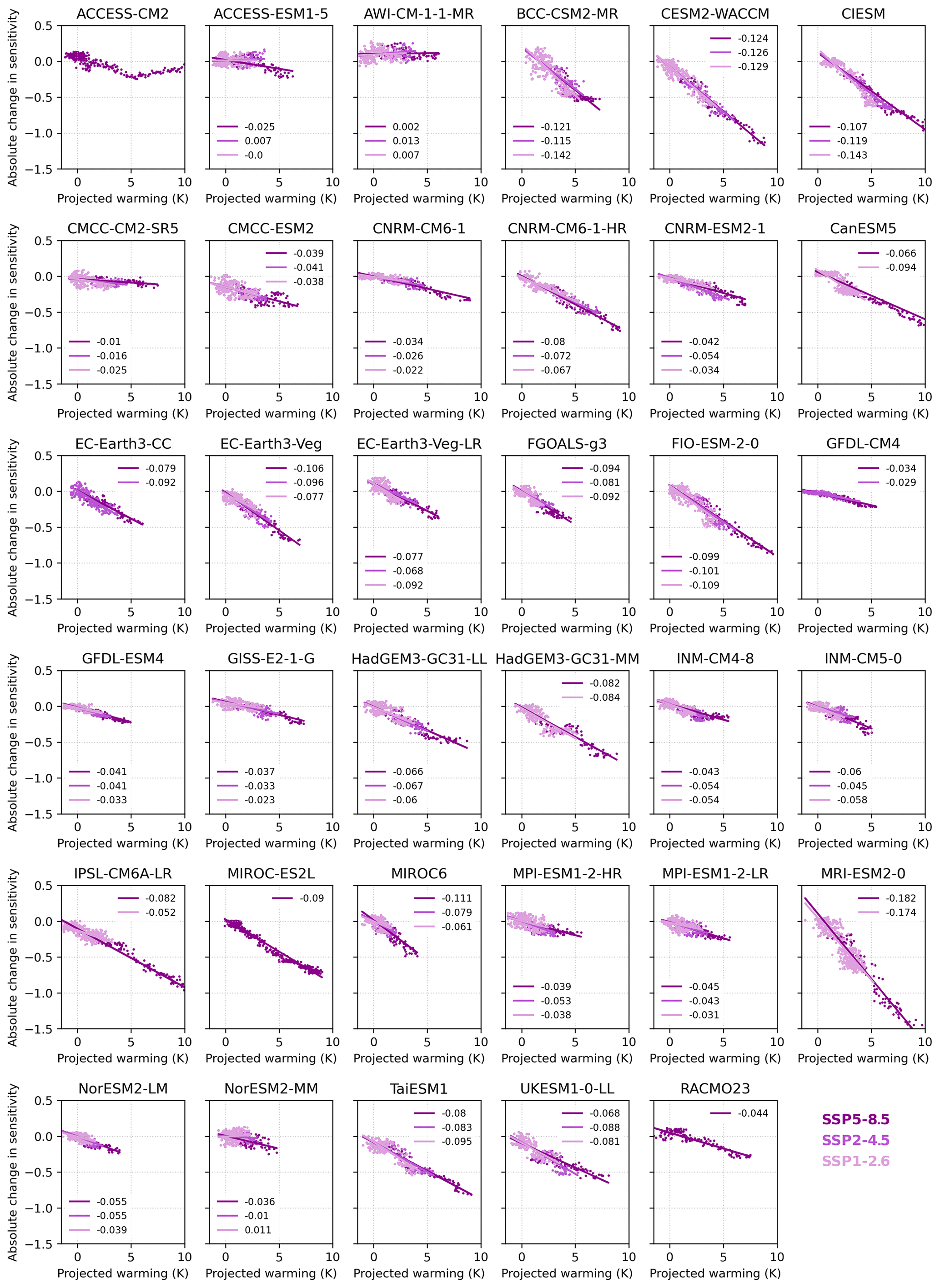
Figure A5 Decrease in the sensitivity factor from spatial regression with warming. In most models we find for rising temperatures a strong decrease in the sensitivity of Antarctic precipitation to local air temperatures. Results are based on the entire time series available for each of the individual models.

Table A1 Model-specific results. We perform a sensitivity analysis with the evolution of log-scaled mean annual precipitation and mean annual air temperature (both continent-wide estimates) over the time period 1850–2100 using different SSP scenarios.

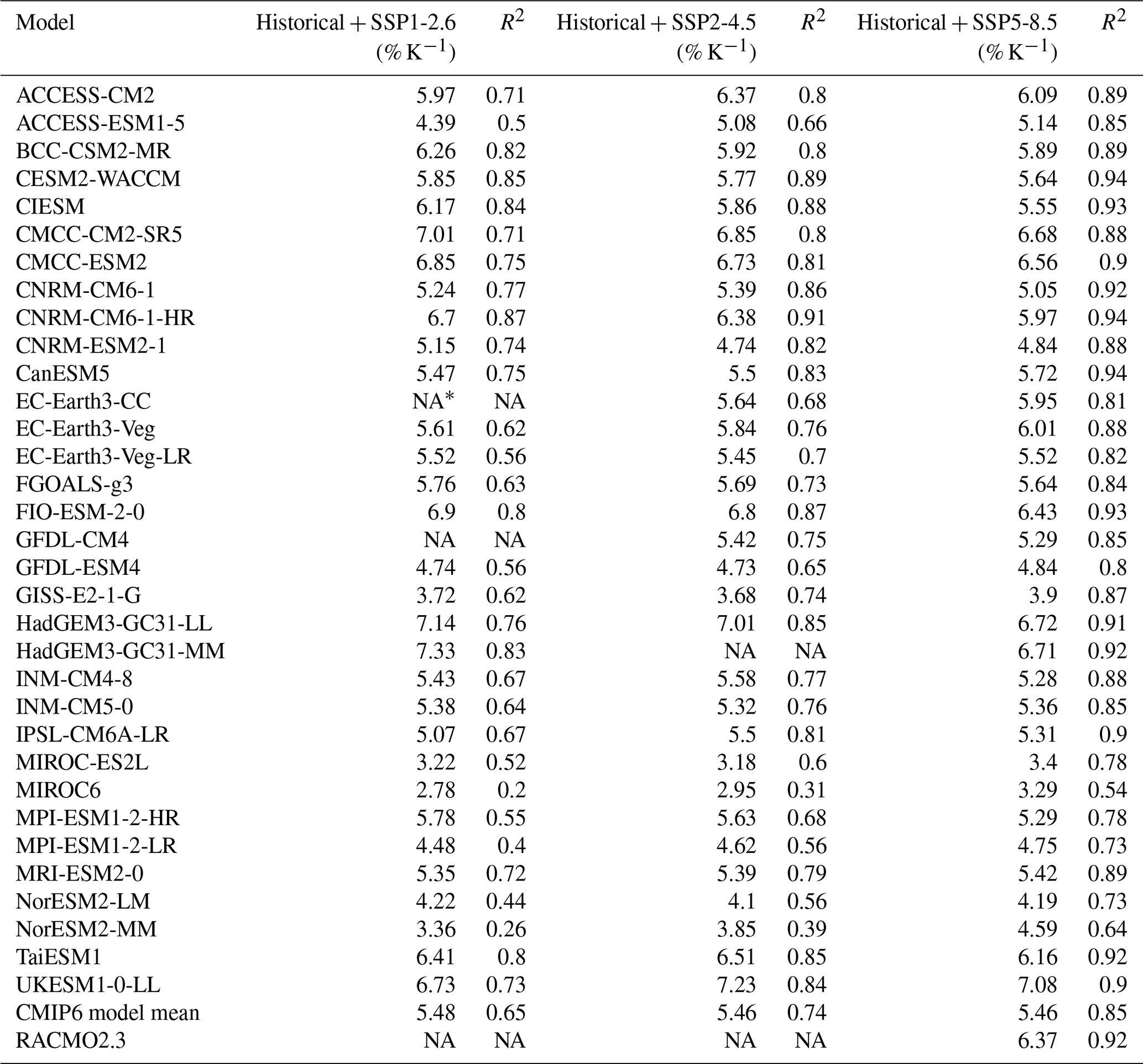
^* NA: not available