the Creative Commons Attribution 4.0 License.
the Creative Commons Attribution 4.0 License.
 | 12 Jun 2023
Strategies for regional modeling of surface mass balance at the Monte Sarmiento Massif, Tierra del Fuego
David Farías-Barahona
Thorsten Seehaus
Ricardo Jaña
Jorge Arigony-Neto
Inti Gonzalez
Anselm Arndt
Tobias Sauter
Christoph Schneider
Johannes J. Fürst
This study investigates strategies for calibration of surface mass balance (SMB) models in the Monte Sarmiento Massif (MSM), Tierra del Fuego, with the goal of achieving realistic simulations of the regional SMB. Applied calibration strategies range from a local single-glacier calibration to a regional calibration with the inclusion of a snowdrift parameterization. We apply four SMB models of different complexity. In this way, we examine the model transferability in space, the benefit of regional mass change observations and the advantage of increasing the complexity level regarding included processes. Measurements include ablation and ice thickness observations at Schiaparelli Glacier as well as elevation changes and flow velocity from satellite data for the entire study site. Performance of simulated SMB is validated against geodetic mass changes and stake observations of surface melting. Results show that transferring SMB models in space is a challenge, and common practices can produce distinctly biased estimates. Model performance can be significantly improved by the use of remotely sensed regional observations. Furthermore, we have shown that snowdrift does play an important role in the SMB in the Cordillera Darwin, where strong and consistent winds prevail. The massif-wide average annual SMB between 2000 and 2022 falls between −0.28 and −0.07 m w.e. yr−1, depending on the applied model. The SMB is mainly controlled by surface melting and snowfall. The model intercomparison does not indicate one obviously best-suited model for SMB simulations in the MSM.
- Article
(5564 KB) - Full-text XML
-
Supplement
(2692 KB) - BibTeX
- EndNote


Together with the Northern Patagonian Icefield and the Southern Patagonian Icefield, the Cordillera Darwin Icefield (CDI) in Tierra del Fuego has experienced strong losses during the last few decades (Rignot et al., 2003; Willis et al., 2012; Melkonian et al., 2013; Braun et al., 2019; Dussaillant et al., 2019). The glaciers of Tierra del Fuego contributed about 5 % of the total glacier mass loss in South America between 2000 and 2011/2014, with a mean annual mass balance (MB) rate of m water equivalent per year (w.e. yr−1) (Braun et al., 2019). However, the difficult accessibility of Patagonian glaciers and the harsh conditions result in scarce in situ observations of glacier MB (Lopez et al., 2010). The Cordillera Darwin especially remains poorly explored (Lopez et al., 2010; Gacitúa et al., 2021).
The CDI is the third-largest temperate ice field in the Southern Hemisphere, with an area of 2606 km2 (state in 2014) including neighboring ice bodies that are not directly connected to the main ice body (Bown et al., 2014). It is located in the southernmost part of the Andes in Tierra del Fuego (Fig. 1) spanning about 200 km in the zonal direction (71.8–68.5∘ W) and 50 km in the meridional direction (54.9–54.2∘ S). The two most prominent peaks are Monte Darwin (also known as Monte Shipton) (2568 m above sea level – a.s.l.) and Monte Sarmiento (2207 m a.s.l.) (Rada and Martinez, 2022). The climate in the Cordillera Darwin is strongly influenced by the year-round prevailing westerlies, which reach a maximum intensity in austral summer. Within the so-called storm track of the westerly belt, frontal systems pass over the region, inducing abundant precipitation (Garreaud et al., 2009). The interaction of these moist air masses with the topography causes intense precipitation over the western side and rain-shadow effects and decreasing precipitation amounts towards the east (Porter and Santana, 2003; Strelin et al., 2008). In the westernmost region of the Cordillera Darwin lies Monte Sarmiento. The study site comprises two ice fields of around 70 and 39 km2 (Barcaza et al., 2017), respectively (Fig. 1), which we group together as the Monte Sarmiento Massif (MSM) in this study. Similar to the large ice fields in Patagonia, studies show that most of the glaciers in this region have experienced glacier thinning and retreat in the last few decades as well (Strelin et al., 2008; Melkonian et al., 2013; Meier et al., 2019).
Many glaciers in southern Patagonia, including the Cordillera Darwin, largely advanced during the Little Ice Age cold interval, with maximum advances in the 16th to 19th centuries (Villalba et al., 2003; Glasser et al., 2004; Strelin et al., 2008; Masiokas et al., 2009; Koch, 2015; Meier et al., 2019). In the last few decades, most glaciers in Patagonia and Tierra del Fuego have been strongly losing mass (Rignot et al., 2003; Strelin and Iturraspe, 2007; Strelin et al., 2008; Willis et al., 2012; Melkonian et al., 2013; Braun et al., 2019; Dussaillant et al., 2019). Thinning rates in the Cordillera Darwin were analyzed for the first time by Melkonian et al. (2013), with an average annual thinning of m yr−1 (2001–2011). More recent studies focused on the Andes estimate average annual thinning in Tierra del Fuego around m yr−1 (2000–2011/2014) (Braun et al., 2019) and m yr−1 (2000–2016) (Dussaillant et al., 2019). Average thinning rates are found to be distinctly higher in the northeastern part compared to the southwestern part due to the strong precipitation gradient across the mountain range (Melkonian et al., 2013). For individual glaciers in the south (e.g., Garibaldi Glacier), Melkonian et al. (2013) even noticed slight thickening.
Simulating glacier melt ranges from empirical approaches to complex energy balance models including many physical details. The former relates melt rates to air temperature, requiring little input. Energy balance models compute all relevant energy fluxes at the glacier surface, thus relying on numerous meteorological and surface input variables (Gabbi et al., 2014). In between, there is a wide range of different complex implementations. To improve the representation of the spatial and diurnal variability of melt, radiation has been included in temperature index models (e.g., Hock, 1999; Pellicciotti et al., 2005). Previous studies (e.g., Six et al., 2009; Gabbi et al., 2014; Réveillet et al., 2017) have shown that physically based models can give accurate results when local high-quality meteorological measurements exist; however, when remote meteorological data or reanalysis data are used, the performance decreases rapidly (Gabbi et al., 2014). Thus, more complex models might not be the optimal choice for areas with limited in situ meteorological measurements, like the Cordillera Darwin. As Patagonian glacier evolution is highly correlated with air temperature (Strelin and Iturraspe, 2007; Weidemann et al., 2020; Mutz and Aschauer, 2022), it is likely that a temperature-based model is able to sufficiently reproduce glacier behavior in the Cordillera Darwin.
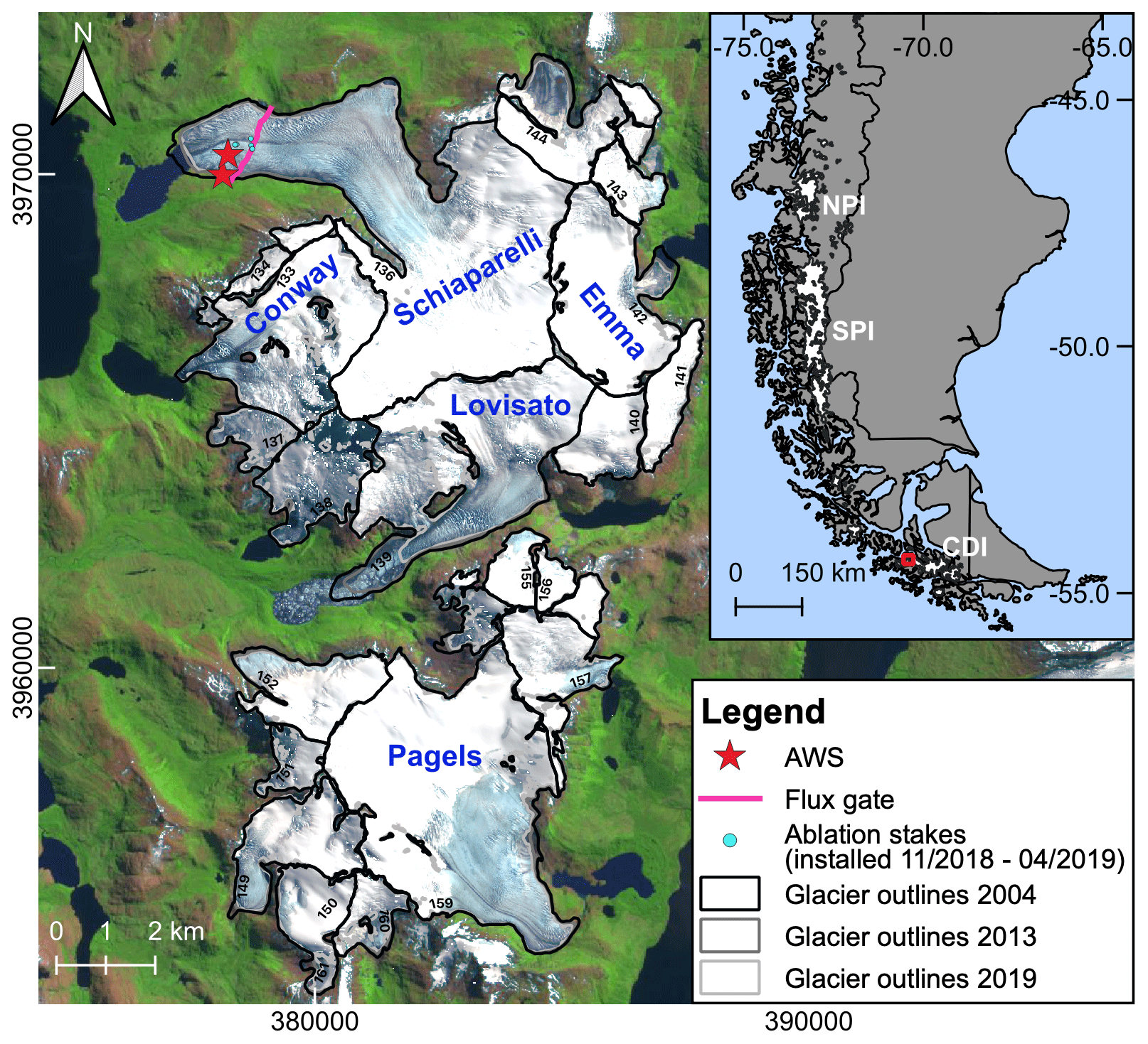
Figure 1Overview of the study site and a subset of the available in situ measurements at Schiaparelli Glacier. The inset map displays Patagonia and its ice fields: the Northern Patagonian Icefield (NPI), Southern Patagonian Icefield (SPI) and Cordillera Darwin Icefield (CDI). The numbers inside the catchment areas refer to the respective glacier ID. Glacier outlines mark the 2004, 2013 and 2019 extents. The satellite image is from Sentinel-2 (4 February 2019) with coordinates in UTM projection, zone 19S.
In order to answer the question of which models are able to reproduce the MB under these unique climatic conditions, we apply four surface mass balance (SMB) models of different complexity at the MSM: (a) a positive degree-day (PDD) model (Braithwaite 1995), (b) a simplified energy balance (SEB) model (Oerlemans, 2001) using potential insolation, (c) a SEB model using the actual insolation (accounting for cloud cover, shading effects and diffuse radiation) and (d) the physically based COupled Snowpack and Ice surface energy and mass balance model in PYthon (COSIPY) (Sauter et al., 2020).
The SMB is given by surface ablation and accumulation. Accumulation is typically considered to equal solid precipitation. However, it also depends on deposition, meltwater percolation and subsequent refreezing as well as on avalanching and snow redistribution by wind. The latter can play a decisive role for the spatial heterogeneity in accumulation of mountain glaciers and can reduce or increase the amount by a large factor (Winstral and Marks, 2002; Lehning et al., 2008; Mott et al., 2008; Dadic et al., 2010; Warscher et al., 2013). In southern Patagonia, where strong winds prevail all year round, we hypothesize that snowdrift has a crucial impact on accumulation and with it on the SMB.
Essential for model performance is an appropriate calibration of model parameters, requiring reliable observations. Parameter tuning has been accomplished with different types of data, ranging from in situ observations of surface ablation and snow properties (e.g., Six et al., 2009; van Pelt et al., 2012; Gabbi et al., 2014; Réveillet et al., 2017; Zolles et al., 2019) to satellite products, e.g., snowline altitudes or mass changes (e.g., Schaefer et al., 2013; Rounce et al., 2020; Barandun et al., 2021). As continuous SMB monitoring is challenging over larger spatial scales covering multiple glaciers, regional modeling attempts often rely on short-term monitoring efforts on a single glacier or a few glaciers (e.g., Schaefer et al., 2013, 2015; Ziemen et al., 2016; Groos et al., 2017; Bown et al., 2019). Though effective, this strategy is in contrast to our knowledge that relations between the atmospheric conditions and the surface melt are highly variable in space and time (Pellicciotti et al., 2005, 2008; MacDougall and Flowers, 2011; Gurgiser et al., 2013; Sauter and Galos, 2016; Réveillet et al., 2017; Zolles et al., 2019). Thus, this common approach inherently implies important uncertainties in the SMB estimate and decreases model performance. Discrepancies become evident when modeling results are compared to independent values on specific mass loss from glaciological or geodetic observations. Such comparisons are often inherent in glacier or ice sheet mass budgeting using various techniques (e.g., Bentley, 2009; Minowa et al., 2021).
The overall goal in this study is therefore to assess and give advice on various strategies for SMB model calibration in the Cordillera Darwin with the aim of achieving reliable simulations of the regional SMB. This objective entails several more specific questions that we want to answer:
-
Q1. Does a single-glacier calibration ensure transferability of the model producing appropriate regional SMB estimates?
-
Q2. Is it beneficial to ingest regional geodetic mass change observations into the SMB model calibration?
-
Q3. Can the performance of the SMB model be improved by increasing the complexity level regarding included processes?
The study is structured as follows: Sects. 2 and 3 describe the study site, data, methods and experimental design. In Sect. 4, we describe the model performance using different calibration strategies and the main characteristics of the SMB in the MSM together with the differences between the employed SMB model types. Section 5 provides a discussion of these results and assesses the main limitations and challenges. In Sect. 6, we summarize the main conclusions.
2.1 The Monte Sarmiento Massif
The main pyramidal summit, Monte Sarmiento, reaches 2207 m a.s.l. Several glaciers descend from all sides of the MSM, together covering ∼70 km2 (Barcaza et al., 2017). To the south of the MSM, another glacierized area of 39 km2 is centered around Pico Marumby (1253 m a.s.l.). Both ice bodies together represent the MSM study area in this study (Fig. 1). The larger ice field includes both land- and lake-terminating glaciers, whereas the smaller one consists entirely of land-terminating glaciers. Schiaparelli Glacier is the largest glacier of the MSM, with an area of 24.3 km2 in 2016 (Meier et al., 2018). It descends Monte Sarmiento to the northwest almost to sea level and calves into a moraine-dammed proglacial lake, which was formed after strong recession in the 1940s (Meier et al., 2019). Meier et al. (2019) found a continuous average glacier retreat of approximately 5 m yr−1 from 1973 to 2018. Analysis of the surface energy and mass balance of Schiaparelli Glacier with a physically based energy balance model revealed a glacier-wide mean annual climatic mass balance of m w.e. yr−1 in 2000–2017 (Weidemann et al., 2020). The mass balance is dominated by surface melt and precipitation (Weidemann et al., 2020).
The largest glaciers in the study site after Schiaparelli are Pagels, Lovisato, Conway and Emma glaciers. Emma Glacier was the target for studying Holocene glaciation in the MSM, which indicated that the Holocene glacier behavior in Tierra del Fuego and southern Patagonia responds synchronously to the same regional climate change (Strelin et al., 2008). The other glaciers in the MSM are largely unsurveyed, except by remote sensing (Melkonian et al., 2013; Braun et al., 2019; Dussaillant et al., 2019). From the geodetic MB data from previous studies, different patterns are observed. Despite the rather small study site and proximity of the glaciers, the characteristics of the geodetic MB in 2000–2013 (see Sect. 2.4) are very heterogenous (Fig. 2). Lovisato Glacier shows by far the highest mass loss. Satellite images (see Fig. 1) reveal large numbers of icebergs in the proglacial lake, indicating significant calving losses for this glacier. A clear contrast between lake- and land-terminating glaciers is not visible. There are several lake-terminating glaciers in the northern part of the study site (Schiaparelli, Conway, 138, Lovisato); however, land-terminating glaciers in this area show similar MBs. Geodetic MBs are also heterogenous in the southern part of the study site, despite all the glaciers being land-terminating.
2.2 In situ observations at Schiaparelli Glacier
We use observational data of two automatic weather stations (AWSs) at Schiaparelli Glacier (Fig. 1). AWS Rock (92 m a.s.l.) is located on rock close to the glacier front. Since the installation in September 2015, it has been measuring air temperature T, relative humidity RH, global radiation G, wind speed U, wind direction DIR and precipitation RRR at hourly resolution. Bucket-based precipitation measurements often show undercatch due to wind and snow (Rasmussen et al., 2012; Buisán et al., 2017), specifically if the bucket is not heated as in this case. Due to the high wind velocities, precipitation measurements are known to be specifically error-prone in Patagonia (Schneider et al., 2003; Weidemann et al., 2018b; Temme et al., 2020). We therefore assume that the measurement instrument only records a fraction of the total precipitation and, thus, the annual amount needs to be increased by 20 %. AWS Glacier (140 m a.s.l. in September 2016) is located on ice in the ablation area of Schiaparelli Glacier. It has been measuring T, RH, G, U, DIR and air pressure PRES at hourly resolution since August 2013 to the present, with some interruptions. Since this AWS is subject to tilting due to melting of the ice surface, we do not use measurements that require a horizontal sensor orientation from this station. In addition, we identified a step change and a multiannual drift in the RH measurements. These measurements were therefore discarded. RH values at AWS Glacier were inferred from AWS Rock assuming identical specific humidity. Values of T, corrected RH and PRES from AWS Glacier are used to inform the statistical downscaling. G and RRR from AWS Rock serve to evaluate modeled radiation and precipitation.
Several ablation stakes, concentrated in the lowest part of the ablation area, deliver information about surface melt. Stakes have been installed at varying locations and for irregular time spans ranging from a few months to almost 1 year. The largest number of stakes was installed in the period November 2018–April 2019 with six stakes at the same time (see Fig. 1). In the other periods the number of measured stakes ranges from one to four (see Fig. S4 in the Supplement). The stake located next to AWS Glacier has been in use for the longest period between August 2013 and April 2019. Additionally, an automatic ablation sensor measured every 150 mm of melt (recording the time point when 150 mm melted) from September 2016 to November 2017, giving temporally higher-resolved information about surface melt.
In April 2016 the ice thickness was measured with a ground-penetrating radar in the ablation area approximately parallel to the glacier front of Schiaparelli Glacier (Fig. 1). Measurements reveal a maximum ice thickness of 324 m with an estimated uncertainty of around 10 % (Gacitúa et al., 2021).
2.3 Reanalysis data
The ERA5 reanalysis data set is the latest global climate reanalysis product of the European Centre for Medium-Range Weather Forecasts (ECMWF). Being a global data set, ERA5 shows high temporal and spatial resolution with an hourly time step and an approximately 31 km horizontal grid over 137 vertical levels (Hersbach et al., 2020). ERA5 and its previous versions have been successfully applied in modeling studies in Patagonia (e.g., Lenaerts et al., 2014; Bravo et al., 2019b; Sauter, 2020; Temme et al., 2020; Weidemann et al., 2020).
ERA5 data are required to extend the time period for our modeling framework beyond the AWS records. Therefore, we infer the local surface conditions near AWS Glacier from the spatially coarse ERA5 data, averaging the four closest grid points to the AWSs. U and cloud cover fraction N are directly taken from ERA5. For T, RH and PRES, quantile mapping (Gudmundsson et al., 2012) was used to relate ERA5 to AWS data (see Sect. 3.1). For downscaling of precipitation, we use a model of orographic precipitation (see Sect. 3.1). It requires the large-scale precipitation and upwind information about geopotential height, air temperature, wind vectors and relative humidity between 850 and 500 hPa which was extracted in a rectangular domain upstream of the study site (54.0–55.0∘ S, 72.0–71.25∘ W).
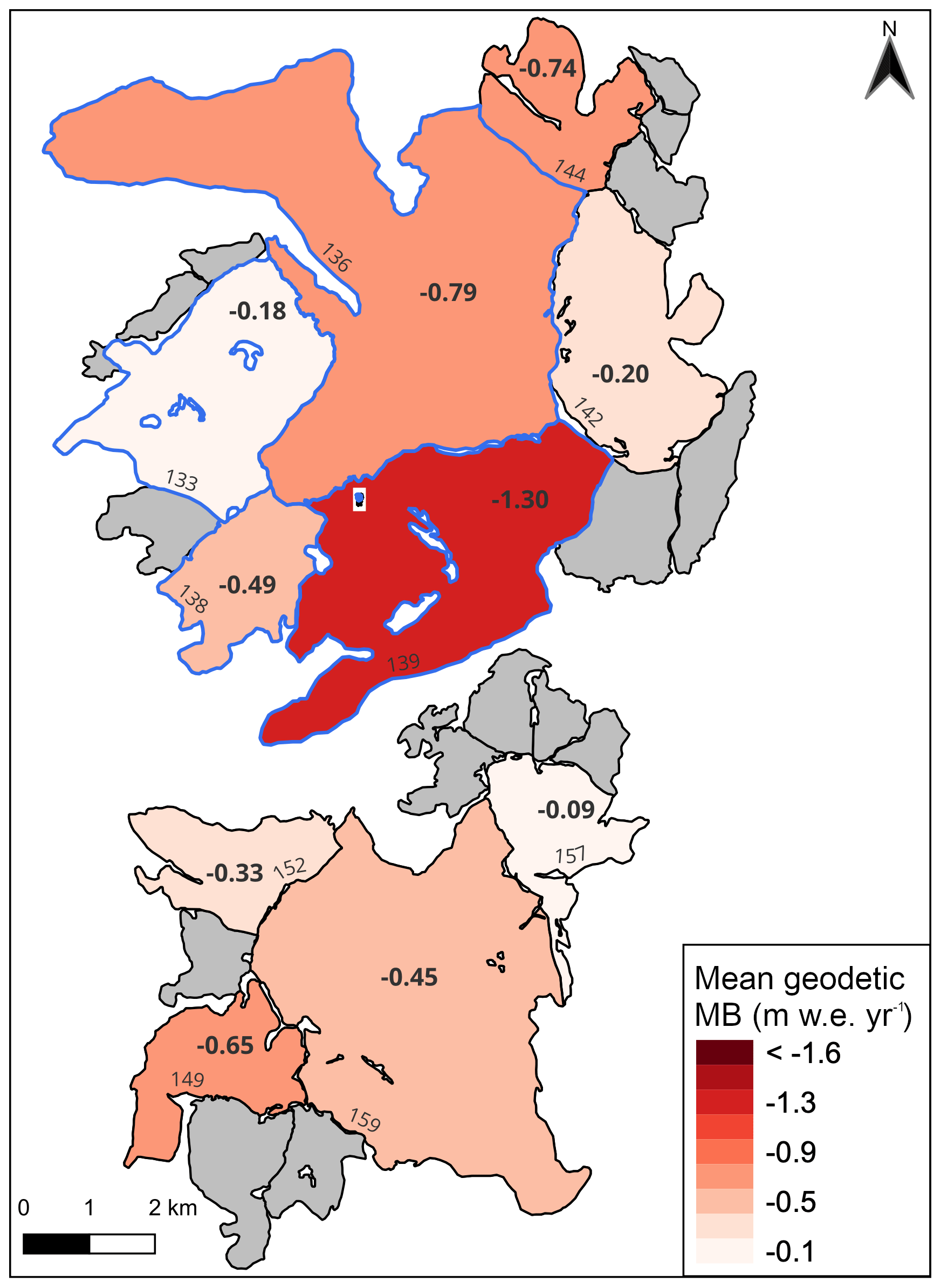
Figure 2Specific geodetic mass balance (MB) from elevation change rates for the individual glaciers (>3 km2) at the MSM study site in 2000–2013. Blue outlines highlight the lake-terminating glaciers. Grey shading indicates glaciers with an area <3 km2. Glacier outlines mark the 2004 extent.
2.4 Remotely sensed data
Glacier outlines from the Monte Sarmiento Massif and their surrounding glaciers are extracted from the two national Chilean inventories generated by the water directorate of Chile (DGA). The first comprehensive glacier inventory of Chile was created from Landsat TM (Thematic Mapper) and ETM+ (Enhanced Thematic Mapper) images acquired in 2004 (Barcaza et al., 2017) and later updated using Sentinel-2 images acquired in 2019 (DGA, 2022). The latter inventory presents an improvement in the glacier catchment areas; however, we observed small inconsistencies in both inventories (ice-covered areas not included in the inventory). Hence, we homogenized both inventories and corrected them. To do so, we used the original and close-date satellite images of both inventories to manually correct these inconsistencies. Moreover, we also generated glacier outlines of 2013 using a composite band of Landsat OLI (Operational Land Imager) images.
We calculate the geodetic MB using digital elevation models (DEMs) from 2000 and 2013. The DEMs from the 2013 TerraSAR-X add-on for the Digital Elevation Measurement mission (TanDEM-X) correspond to a part of the data set generated in the study of Braun et al. (2019), which presents a complete coverage of the study area. Braun et al. (2019) calculated the elevation changes for the entire Tierra del Fuego region from synthetic aperture radar (SAR) DEMs between 2000 and 2011/2015. For this study, the elevation changes were derived from the Shuttle Radar Topography Mission (SRTM) in 2000 and the 2013 TanDEM-X DEMs. In general, the TanDEM-X DEMs were derived using differential SAR interferometry techniques. Details regarding the SAR approach can be found in Braun et al. (2019).
To obtain precise elevation change fields, the TanDEM-X DEMs are horizontally and vertically coregistered to the SRTM (reference) DEM using stable areas (Braun et al., 2019; Sommer et al., 2020). Subsequently, the elevation change differencing is estimated. Data gaps are filled by applying an elevation change versus altitude function by calculating the mean elevation change within 100 m-high bins across the glacier area. Finally, we remove steep slopes () to avoid artificial biases introduced by outliers and filter each elevation band by applying a quantile filter (1 %–99 %) (Seehaus et al., 2019; Sommer et al., 2020).
To estimate the geodetic MB between 2000 and 2013, we use the two corresponding abovementioned glacier inventories to take into account the glacier area loss (Sommer et al., 2020). To convert volume to mass changes, a density factor of 900 kg m−3 is applied.
Errors and uncertainties from the geodetic MB () were calculated using a standard error propagation Eq. (1) from Braun et al. (2019), which considers the following factors.
-
Accuracy of the elevation change rates (considering spatial autocorrelation and hypsometric gap filling) ()
-
Accuracy of the glacier areas (δA) (for this study we will include the accuracy of the two glacier inventories)
-
Uncertainty from volume-to-mass conversion using a fixed density (δρ)
-
Potential bias due to different SAR signal penetration () (details in Braun et al., 2019)
The geodetic MB calculated from the elevation change rates (2000–2013) is presented in Fig. 2. The annual MB is negative throughout the region but with a rather wide range from −1.30 to −0.09 m w.e. yr−1 (Fig. 2).
Multi-mission SAR remote-sensing data were employed to obtain information about glacier speeds. The database covers the period 2001–2021 (ERS-1/2 IM SAR, July–August 2001; ENVISAT ASAR, March–July 2007; ALOS PALSAR, August 2007–September 2010; TerraSAR-X/TanDEM-X, May 2011–February 2021). More detailed information about the sensor specifications can be found in Seehaus et al. (2015).
3.1 Atmospheric forcing
Atmospheric forcing for the SMB models requires T, RH, U, PRES, G, RRR and N. T, RH and PRES are statistically downscaled to the AWS location and subsequently extrapolated over the study site, while U and N are directly taken from ERA5. G and RRR are produced using additional models for radiation and orographic precipitation, respectively. The statistical performance of all input variables compared to AWS measurements is summarized in Table S1 in the Supplement.
Statistical downscaling of T, RH and PRES is performed via quantile mapping. Quantile mapping is a technique for statistical bias correction of climate model outputs by transferring the cumulative distribution function of the model to the cumulative distribution function of the observation (Gudmundsson et al., 2012; Cannon et al., 2015). This technique has been successfully applied in Patagonia before (e.g., Weidemann et al., 2018a, 2020). Statistically downscaled T and PRES are spatially extrapolated from AWS Glacier over the topography using a linear temperature lapse rate (TLR) and the barometric equation, respectively.
G over the glacier surface is modeled based on the radiation scheme of Mölg et al. (2009a). It calculates both the direct and diffuse parts of the incoming solar radiation from N, T, RH and PRES. Radiation is corrected for the slope and aspect of the respective grid cell. Furthermore, both self-shading and topographic shading are considered, and thus shaded grid cells only receive the diffuse component of the incoming solar radiation (Mölg et al., 2009a, b).
As precipitation events can be short-lived and highly variable in space, it is challenging to infer reliable distributions over complex terrain from coarse global data sets. Furthermore, a direct extrapolation of the sparse AWS measurement network in the CDI using altitudinal lapse rates is critical because measurements in this region are error-prone (Schneider et al., 2003, 2007; Temme et al., 2020). Therefore, we follow a physically motivated approach using an orographic precipitation model, which has been successfully used in glaciological studies before (e.g., Schuler et al., 2008; Weidemann et al., 2018a, 2020). The model is based on the linear steady-state theory of orographic precipitation and includes airflow dynamics, cloud timescales and advection and downslope evaporation (Smith and Barstad, 2004; Barstad and Smith, 2005). In this way, the precipitation resulting from forced orographic uplift over a mountain is calculated (Weidemann et al., 2018a). For a more detailed description, see Smith and Barstad (2004), Barstad and Smith (2005) and Sauter (2020).
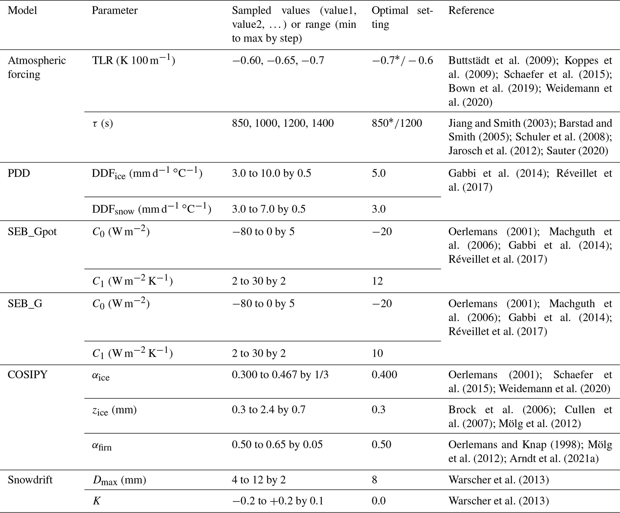
The orographic precipitation model assumes stable and saturated conditions, and thus time intervals that do not fulfill these constraints need to be excluded (Smith and Barstad, 2004; Weidemann et al., 2018a). We use relative humidity, Brunt–Väisälä frequency and Froud number as model constraints in order to ensure saturated, stable airflow without flow blocking. A positive zonal wind component guarantees that airflow crosses the mountains from west to east. The total precipitation is calculated by adding the large-scale precipitation (after removing the orographic component from the ERA5 precipitation) to the orographic precipitation calculated in the model. Based on the annual precipitation amounts from AWS Rock, we are able to constrain the relative humidity threshold (90 %) above which orographic precipitation can occur and the large-scale precipitation from ERA5. In this way, we guarantee that the annual total precipitation at the AWS location agrees with the observed amounts. Conversion and fallout timescales of hydrometeors (τ) are varied within the range of previous studies (Table 1) in the latter model calibration (Jiang and Smith, 2003; Barstad and Smith, 2005; Smith and Evans, 2007; Weidemann et al., 2013, 2018a, 2020; Sauter, 2020).
Table 1Overview of the calibration parameters for the atmospheric forcing and the SMB models. The best values are given for calibration Strategy C (see Sect. 3.5.1). The asterisk (*) indicates deviating values for calibration Strategy A. The specific parameter ranges were inferred from the given references.
3.2 Surface mass balance models
We use four types of SMB models with different complexity. In this way, we can understand which type of model is well-suited and which processes are essential for SMB simulations in the MSM. Calibration parameters for each model are summarized in Table 1. The calibration approach is described in detail in Sect. 3.5.1. For calibration, simulations were limited to the period in which observations are available (April 1999–March 2019). The final SMB simulations have been extended to the period April 1999–March 2022 at the end to produce the most comprehensive and updated results possible. A complete overview of the model setup and fixed parameter values is given in the Supplement (Table S2). In the following we explain the different models.
3.2.1 PDD
Positive degree-day models (Braithwaite, 1995) relate air temperature to surface melt by melt factors that distinguish between ice and snow surfaces. The melt M is calculated by
DDF (mm d−1 ∘C−1) are the degree-day factors for ice and snow, respectively, n is the number of time steps per day (here n=8), Ta is the air temperature and TT is the temperature threshold above which melt occurs (here TT=1.0 ∘C) (Pellicciotti et al., 2005; Gabbi et al., 2014). The model keeps track of the snow depth in each grid cell to decide whether snow or ice is melted. Accumulation occurs as snowfall at locations where air temperature lies below 1.0 ∘C.
3.2.2 SEB_Gpot
In the SEB melt model of Oerlemans (2001), the available melt energy QM is calculated by parameterizing the temperature-dependent energy fluxes with the empirical factors C0 (W m−2) and C1 (W m−2 K−1):
If snow-free, α is set to αice=0.3. The snow albedo is not a fixed value, but it considers the aging and densification processes using a parameterization via air temperatures since the last snowfall event:
where a1 is the albedo of fresh snow (0.9) and a2=0.155 (Pellicciotti et al., 2005).
In this first model variant (SEB_Gpot), the incoming solar radiation I is directly related to the potential insolation Ipot via the atmospheric transmissivity τatm (τatm=0.38) giving . Accumulation occurs as snowfall at locations where air temperature is below 1.0 ∘C.
3.2.3 SEB_G
In order to have a more accurate representation of the incoming solar radiation at each location of the glacier basin, a radiation model is employed. We use the incoming shortwave radiation which we computed with the radiation model based on Mölg et al. (2009a) (see Sect 3.1) as input for a second model variant of the SEB model (SEB_G) (I=G). Using the SEB model with two differently complex sets of radiation information, we are able to analyze the importance of accurate radiation input for SMB modeling.
3.2.4 COSIPY
The open-source model COSIPY (Sauter et al., 2020) is an updated version of the preceding model COSIMA (COupled Snowpack and Ice surface energy and MAss balance model) by Huintjes et al. (2015). COSIPY is based on the concept of energy and mass conservation. It combines a surface energy balance with a multilayer subsurface snow and ice model, where the computed surface meltwater serves as input for the subsurface model (Sauter et al., 2020). In comparison to the previous model types, the primary difference is that the energy fluxes are treated explicitly. Moreover, snow densification as well as meltwater percolation and refreezing in the snow cover are possible. Strictly speaking, COSIPY calculates the climatic mass balance following the definition in Cogley et al. (2011), giving the surface plus the internal mass balance. To maintain readability, we will also stick to the term “surface mass balance” for COSIPY, although we underrate the included processes in COSIPY this way.
The energy balance model combines all energy fluxes F at the glacier surface:
where SWin is the incoming shortwave radiation taken from the radiation model (G) (see Sect 3.1), α is the surface albedo, LWin and LWout are the incoming and outgoing longwave radiation, Qsen and Qlat are the turbulent sensible and latent heat flux, Qg is the ground heat flux and QR is the rain heat flux. Melt only occurs if the surface temperature is at the melting point (0.0 ∘C) and F is positive. Under this condition, the available energy for surface melt QM equals F. Otherwise, this energy is used for changing the near-surface ice or snow temperature. The total ablation comprises not only surface melting, but also sublimation and subsurface melting. Mass gain by accumulation is possible via snowfall, deposition and refreezing. A logistic transfer function is applied to derive snowfall from precipitation scaling around a threshold temperature of 1.0 ∘C.
The albedo is parameterized based on the approach by Oerlemans and Knap (1998), where the snow albedo depends on the time since the last snowfall and the snow depth. The turbulent heat fluxes are parameterized using a bulk approach. COSIPY offers two options to correct the flux–profile relationship by adding a stability correction; we confined ourselves to the Monin–Obukhov similarity theory (Sauter et al., 2020). With sensitivity testing, we found the ice albedo (αice), the roughness length of ice (zice) and the firn albedo (αfirn) to be the most important tuning parameters in the MSM.
3.3 Snowdrift
Redistribution of snow caused by wind plays a key role in the spatial heterogeneity in accumulation. In Tierra del Fuego and Patagonia, where strong winds prevail throughout the year, we hypothesize that snowdrift has a crucial impact on accumulation and the SMB. Thus, a simple parameterization to capture wind-driven snow redistribution based on Warscher et al. (2013) was slightly modified and added to the SMB model types. The scheme determines locations that are sheltered from or exposed to wind by an analysis of the topography and corrects the solid precipitation accordingly:
The correction factor Cwind for each grid cell is calculated by
Dmax gives the maximum deposition in millimeters, dSVF is the directed sky-view factor and K is a calibration constant, which was set to 0.1 by Warscher et al. (2013). We vary it in a range from −0.2 to +0.2 in the snowdrift calibration together with the Dmax (Table 1). E is a factor for weighting with elevation (linearly) ranging from 0 to 1, assuming that lower wind speeds prevail at lower elevations, which reduces the snow redistribution. In this study, we additionally include a weighting with prevailing wind speed U to further improve the performance because we observe different wind directions with different velocities and we suppose that more (less) snow is also redistributed during periods of higher (lower) wind velocities. For a more detailed description of the snowdrift scheme, please refer to Warscher et al. (2013).
3.4 Ice flux and mass budgeting
Ice surface velocity fields are derived from the SAR imagery database by applying intensity offset tracking to co-registered image pairs (Strozzi et al., 2002). Tracking parameters were adjusted depending on sensor specification and acquisition intervals. The tracking is done using multiple tracking patch sizes in order to account for different glacier flow speeds, and a subsequent stacking of the results was applied. More details on the processing, including filtering and error estimation, can be found in Seehaus et al. (2018).
In order to estimate the ice flux, a flux gate was defined along a cross-profile following the thickness surveys in 2016 (Gacitúa et al., 2021). By combining the obtained surface velocity information with the ice thickness measurements along this flux gate, the ice flux was computed following the approach of Seehaus et al. (2015) and Rott et al. (2011). In order to account for ice thickness changes at the flux gate throughout the observation period, the measured ice thickness values were corrected by a surface-lowering rate of −2.8 m yr−1 derived from the annual average elevation change rate between 2000 and 2019 (see Sect. 2.4) near the flux gate. The resulting ice flux through the flux gate is summarized in Table S3.
The combination of the SMB integrated over the glacier area above the flux gate and the mass lost through the flux gate allows us to determine the total mass budget of Schiaparelli Glacier. This value is comparable to the geodetic MB from elevation changes in the area above the flux gate and will be used as one calibration constraint in this study.
3.5 Experimental design
3.5.1 Calibration strategies
We use three different strategies for model calibration that are summarized in Fig. 3. The calibration strategies are based on calculations of model skill. The choice for which parameters enter the calibration was preceded by sensitivity studies on an exhaustive set of parameters with the aim of covering all relevant contributions to SMB. The TLR and τ give control on the amount of snowfall and on temperature-dependent melting. For the PDD and the two SEB variants, we calibrate the model-specific parameters (DDFice and DDFsnow, and C0 and C1, respectively). For COSIPY we must constrain the number of calibrated parameters to limit the modeling effort. Therefore, we decided for the ice albedo (αice) and the roughness length of ice (zice), which constrain ice melting addressing both the radiative and turbulent energy fluxes. To also have a control on the higher-elevated, firn-covered parts of the glaciers, we include the firn albedo (αfirn). Sensitivity testing revealed that those parameters impact the SMB results the strongest. Other parameters we had tested are the temperature of snow/rain transfer, the albedo of snow, the albedo time constant which gives the effect of ageing on the snow albedo and the method of stability correction. Those parameters were fixed at the end because they either were interdependent with other parameters, had a minor impact on the overall results or showed a clear advantage of the one method.
In Strategy A, calibration is focused only on Schiaparelli Glacier, where we have in situ observations. These include ablation stake measurements (see Sect. 2.2) and estimation of the total glacier mass budget using a combination of elevation changes and mass flux through a flux gate parallel to the glacier front (see Sect. 3.4). Measured melt at each ablation stake is compared to modeled average melt at all grid cells of the same altitude (±5 m) at Schiaparelli Glacier for the respective same period. Ablation measurements give control on the processes of melting in the ablation area, whereas the mass budget gives an additional control on the basin-wide mass overturning and with it on the amount of accumulation. After this glacier-specific calibration, the model is transferred to regional scales, i.e., the surrounding glaciers in the study site, with the parameter setting we found in the calibration.
In Strategy B, we use regional geodetic MB observations from MSM elevation changes (2000–2013). In this way, we calibrate the SMB model towards the massif-wide average in order to guarantee that the total net amount of accumulation and ablation on a regional scale is close to observations. Since dynamical losses at calving fronts are not considered in the SMB but are included in the geodetic MB, we exclude glaciers that have significant calving losses (Lovisato Glacier). However, we include glaciers in the average value that are lake-terminating but known to have only minor calving losses. Furthermore, only glaciers larger than 3 km2 are considered because small glaciers involve larger uncertainties. The average annual MB of this subset of glaciers is referred to as BMSMnc in the following and comprises around 71 % of the total glaciated area. The annual average SMB of the corresponding glaciers is then calibrated towards this observed value.
In Strategy C, we follow Strategy B but additionally activate a snowdrift module that needs to be calibrated in this step. After defining the regional massif-wide amount of accumulation in Strategy B, we now optimize the distribution of snowfall on the local scale with the inclusion of the snowdrift. As calibration constraints, we again rely on the BMSMnc but additionally consider the total mass budget of Schiaparelli Glacier to incorporate information about local distribution of snow. We ensure mass conservation by keeping the total amount of snowfall nearly (±10 %) constant.
We use the PDD for calibration of the climate- and snowdrift-related parameters. These include the TLR and τ as well as Dmax and K. Additional model-specific parameters are DDFice and DDFsnow. The number of varied parameters and their ranges are based on what has been used in previous studies (see Table 1). For the other three models, we fix the temperature and precipitation field and the snowdrift parameters based on the results of the PDD calibration. In this way, we guarantee consistency in the atmospheric forcing and save computational cost. Thus, only model-specific parameters are calibrated for those following Strategy C (see Fig. 3).
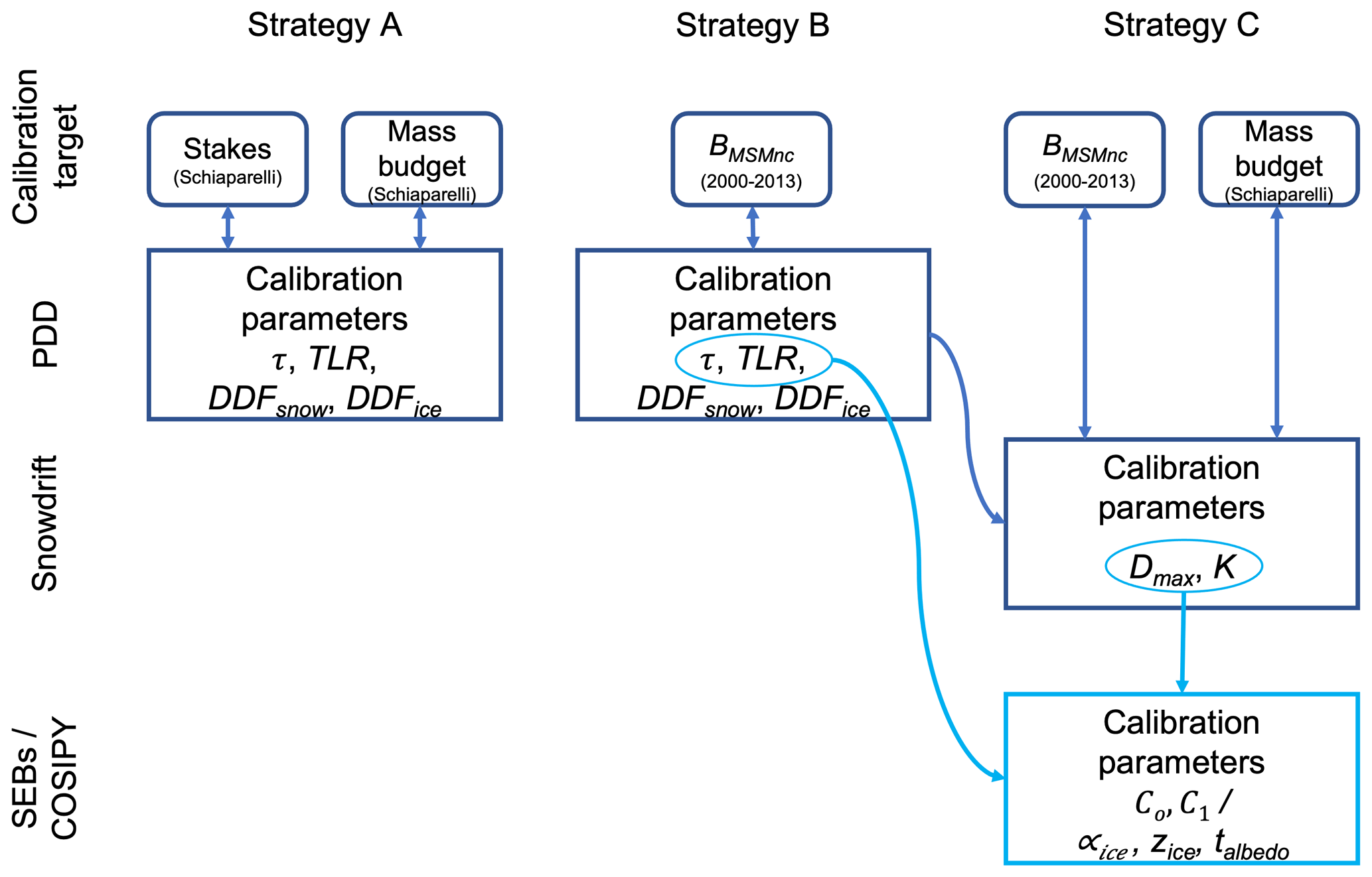
Figure 3Overview of the three calibration strategies used for the calibration of the PDD model, the snowdrift module and the final calibration of SEB_Gpot, SEB_G and COSIPY.
The model skill is calculated using different combinations of observations, depending on the respective calibration strategy. These include the ablation stake measurements at Schiaparelli Glacier, the total mass budget of Schiaparelli Glacier and the geodetic MB derived from elevation changes on a massif-wide average (glaciers >3 km2) excluding significantly calving glaciers (BMSMnc). To calculate the model skill for each run, the simple averaging method of Pollard et al. (2016) is used by applying full-factorial sampling. Taking the misfit between model and observation, an objective aggregate score is determined (Pollard et al., 2016; Albrecht et al., 2020). The misfits are calculated by mean squared errors between observation and model. Thereby, the individual, normalized score Si,j is obtained for each considered measurement type i and each parameter sample j (see Table 1):
Here, is the median of all misfits of one measurement type (for all parameter combinations). The unweighted, aggregated score for each run is the product of the individual scores:
The run with the highest aggregated score Sj implies the optimal parameter combination.
3.5.2 Model evaluation and intercomparison
To investigate the model performance, we compare the modeled surface and observed geodetic MB of the individual land-terminating glacier basins (>3 km2) at the study site (2000–2013). To determine the agreement, we compute the area-weighted root mean square error (RMSE). Furthermore, we assess the agreement between modeled and observed ablation at the ablation stakes in the observation period between 2013 and 2019.
In order to investigate the performance of SMB models with a different degree of complexity, we compare the results of four model types. After calibrating the model-specific parameters of each model individually, the best-guess SMB characteristics and uncertainties of each model can be compared with each other with respect to the observed geodetic MBs. Uncertainties and sensitivity to the calibration parameters are discussed in the Supplement.
4.1 Strategies for model calibration
4.1.1 Strategy A: single-glacier calibration
Results of model calibration show that ablation stake measurements give a control on melting only since almost no snowfall occurs at the stake locations. Thus, the ability to reproduce ablation at the stakes depends principally on the DDFice (see Fig. S1a, b). The total mass budget, additionally, depends strongly on the TLR and τ and thus both the ablation and the distribution and amount of snowfall over elevation (see Fig. S1c). Based on this information, we are able to narrow down the amount of solid precipitation. The combination of both data sets allows an accurate calibration of ablation at Schiaparelli Glacier and a well-informed estimate of precipitation amounts over its catchment area.
An overview of the calibration scores for Strategy A is presented in Fig. S1d. This strategy suggests a TLR of −0.70 ∘C 100 m−1 at Schiaparelli Glacier. The requirement for a higher TLR tells us that a steeper SMB gradient with respect to elevation is needed in order to meet the observations, resulting in reduced ablation with altitude and increased snowfall. A similar signal comes from the τ, where a value of 850 s is most suitable, producing a precipitation field with a high amount of orographic precipitation. The degree-day factors DDFice and DDFsnow are set to 6.0 and 3.0 mm d−1 ∘C−1, respectively.
After the local calibration at Schiaparelli Glacier, the model is transferred to the surrounding glaciers. The results are given in Table 2. Comparing the surface (−0.62 m w.e. yr−1) and the geodetic MB (−0.79 m w.e. yr−1) delivers an estimated calving flux of 0.17 m w.e. yr−1 (4.26 Mt yr−1) at Schiaparelli Glacier. However, the application on the regional scale shows that the SMB is consistently overestimated compared to the geodetic observations (Fig. 4). The observed value for the BMSMnc of −0.51 m w.e. yr−1 is even positive, with +0.09 m w.e. yr−1 in the model (Table 2). Furthermore, several land-terminating glaciers, where no calving losses are involved, have a clearly positive annual SMB which differs distinctly from the observations. The poor agreement is reflected in a high RMSE of 0.56 m w.e. yr−1 (Table 2).
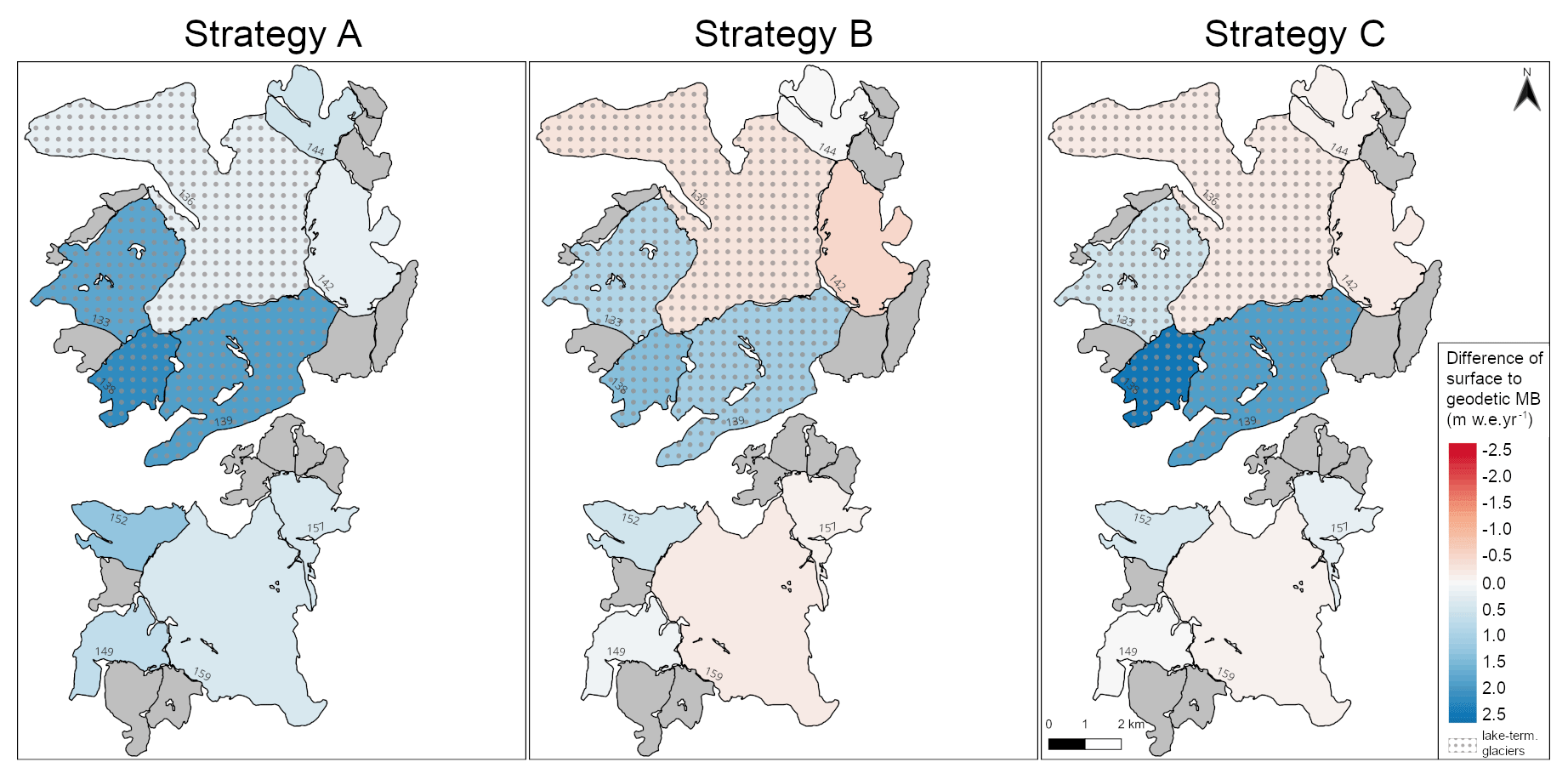
Figure 4Difference of modeled surface to observed geodetic MB (2000–2013) for the three calibration strategies. Dotted areas indicate lake termination precluding a direct comparison of the two data sets. Grey shading indicates glaciers with an area <3 km2. Glacier outlines mark the 2004 extent.
4.1.2 Strategy B: regional calibration
In a second strategy, we use the regional geodetic MB as the sole calibration target. Therefore, we rely on the massif-wide average annual geodetic MB obtained from satellite observations, excluding glaciers with major calving losses (BMSMnc) (see Fig. S1e). Following the approach in Strategy A, the model calibration is performed with the PDD calibrating the same parameters again. While the DDFice updates to 5.0 mm d−1 ∘C−1, the DDFsnow remains unchanged. The TLR changes to −0.60 ∘C 100 m−1 and the τ to 1200 s. Accordingly, the amount of precipitation and the ratio of solid and liquid precipitation are shifted towards less snowfall.
Using regional observations of geodetic MB from satellite data, the calibration for a regional application can be improved. As it is the sole calibration target, the value of the BMSMnc is reproduced perfectly with a modeled value of −0.51 m w.e. yr−1 (Table 2). Individual glaciers show a loss of performance: e.g., at Schiaparelli Glacier, the simulated SMB becomes more negative. However, looking at several land-terminating glaciers of the MSM (glaciers 149, 152 and 159), the agreement has considerably increased (Fig. 4). This is also reflected in a strong decrease in the RMSE to 0.30 m w.e. yr−1 (Table 2). The positive SMB bias from calibration Strategy A is no longer discernible.
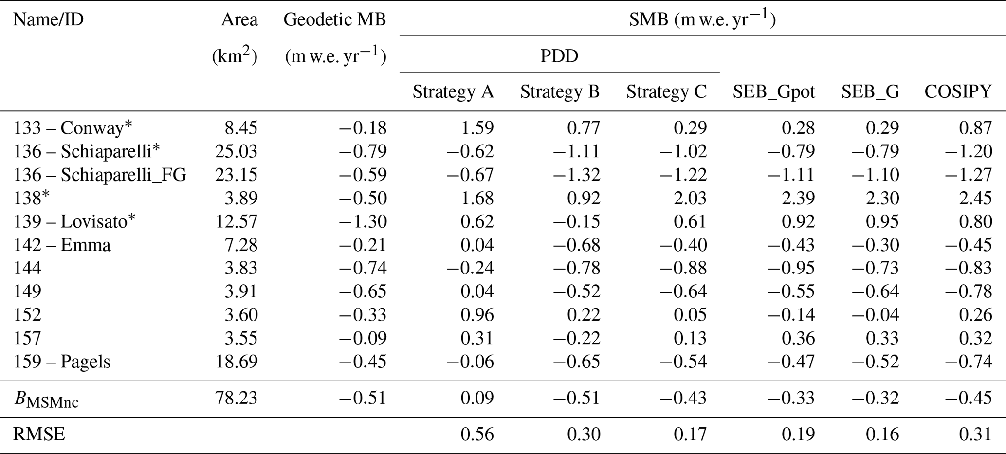
Table 2Comparison of modeled surface to observed geodetic MB (m w.e. yr−1) (2000–2013) from the PDD using three different calibration strategies and from SEB_Gpot, SEB_G and COSIPY for the glaciers at the study site (>3 km2). The results of Strategy C equal the final results of the PDD model. BMSMnc gives the massif-wide annual-average MB excluding glaciers with major calving losses. The root mean square error (RMSE) is weighted by area and calculated from the land-terminating glaciers. The asterisk marks lake termination.
4.1.3 Strategy C: regional calibration including snowdrift
Adding snowdrift delivers additional parameters that need to be calibrated with the PDD. Therefore, we fix the model parameters as determined in Strategy B. Afterwards, the snowdrift parameters are calibrated, suggesting a Dmax of 8.0 mm and a K of +0.0. The snowdrift scheme redistributes snow on average from the northwest to the southeast of the massif due to prevailing northwesterly flow. Subsequently, the southeastern glaciers obtain higher snowfall amounts, whereas from the northwestern glaciers snow is on average removed. With this procedure the agreement between modeled and observed MBs is further improved (Fig. 4), although the resulting simulated BMSMnc (−0.43 m w.e. yr−1) is slightly overestimated (Table 2). At Schiaparelli Glacier, where a large part of the accumulation area is located east of the prominent Monte Sarmiento, snow is on average deposited, producing a slightly less negative SMB, which is closer to observations. For the land-terminating glaciers, the difference between model and observations now lies close to the uncertainty of the observation (Table S5), with a total RMSE of 0.17 m w.e. yr−1. Therefore, further tuning is neither required nor justifiable.
The other three SMB models are limited to calibration Strategy C for the sake of computational cost. We use the TLR, τ and snowdrift parameters as found by the PDD and calibrate the model-specific parameters only (see Table 1, Fig. S2). For the SEB_Gpot/SEB_G, we get a C0 and C1 of −20 W m−2 and 12/10 W m−2 ∘C−1, respectively. COSIPY calibration reveals an αice of 0.4, an αfirn of 0.5 and a zice of 0.3 mm.
4.2 Surface mass balance of the Monte Sarmiento Massif
Generally, all four models give very similar results of SMB (Fig. 5). The spatial distribution and seasonal/interannual patterns are captured by all the models in a similar way. We will summarize the main characteristics of SMB in the MSM in the following and highlight differences between the models. For this analysis, we include all glaciers at the study site (no area limit) to produce the most comprehensive results possible.
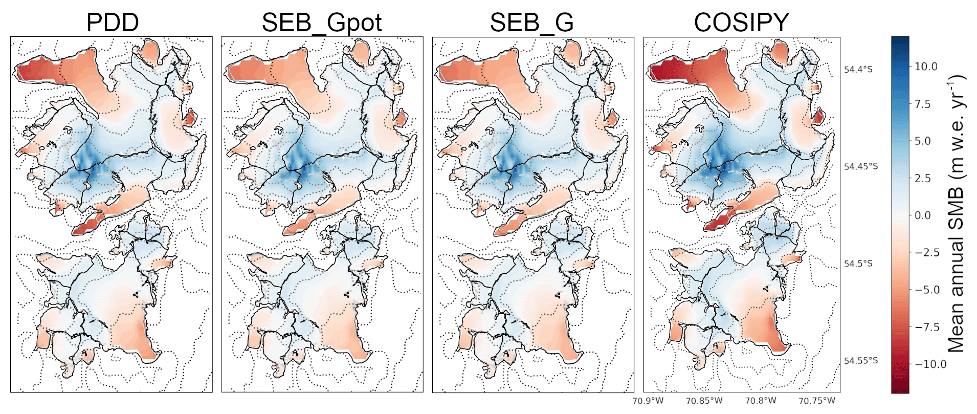
Figure 5Mean annual surface MB (SMB) for the four SMB models (2000–2022). Dotted lines mark altitude in 300 m intervals with intensity decreasing with height. Glacier outlines represent 2004 (black), 2013 (dark-grey) and 2019 (light-grey) extents.
The massif-wide average annual SMB lies just below equilibrium, with the PDD and COSIPY producing more negative values (−0.28 and −0.20 m w.e. yr−1, respectively) than the SEB_Gpot and SEB_G (−0.07 and −0.13 m w.e. yr−1, respectively). For all the models, the SMB is mainly influenced by snowfall (average of +1.66 to +1.79 m w.e. yr−1) and melt (average of −1.87 to −2.55 m w.e. yr−1). Snowfall is almost zero in the lowest parts of the glaciers, indicating melt all year round (Fig. S3). The distribution of snow reflects the topography, increasing strongly towards the summits and showing the largest snow deposition southeast of the mountain peaks and ridges. The highest amounts are found on the wind-sheltered slopes of the Monte Sarmiento summit. For all four SMB models, we see high mass gain due to snowfall in the elevated areas of the massif (up to around 10 m w.e. yr−1) and extreme mass loss at the glacier tongues (up to around −10 m w.e. yr−1) (Fig. 5). Several glaciers have large ablation areas (Schiaparelli, Lovisato, Pagels). However, Schiaparelli Glacier stands out due to its large size, the range of altitude and its huge glacier tongue causing a much larger area of intense ablation compared to the other glaciers in the region. Depending on the model type, the massif-wide equilibrium line altitude is on average between 770 and 794 m a.s.l. during the study period. Equilibrium line altitudes tend to be lower in the east of the massif compared to the west, which can be confirmed by snowline altitudes from satellite observations in the region (Table S4).
Due to the location at the higher mid latitudes, the seasonal variations are huge. In summer, the average SMB is negative up to around 900–1000 m a.s.l., which leaves (almost) no area of mass gain for several glaciers in the region (see Fig. S3). This applies in particular to the southern, lower-elevation massif. In winter, the majority of the MSM area is characterized by a positive SMB. The cooler temperatures cause higher snowfall amounts, and we also observe snowfall over lower altitudes (see Fig. S3). More than 65 % of the total snow accumulates in winter (June to August) and spring (September to November) but only 13 % in summer (December to February).
Over the course of the 22-year study period, we see a phase of more negative and more positive annual SMB that all four models agree on (Fig. 6). Massif-wide, more positive MB values prevail between 2009 and 2015/16, with more negative ones before and after this phase. More negative MBs coincide with over-average temperatures and decreased snowfall and vice versa. All the models agree that the most negative MBs likely occurred in 2003/04, 2005/06, 2016/17, 2019/20 and 2020/21. However, the amplitude of annual mass balances differs significantly between the models. Overall, the PDD and COSIPY tend to simulate more negative MBs; however, COSIPY also simulates more positive MB in several positive years (Fig. 6).
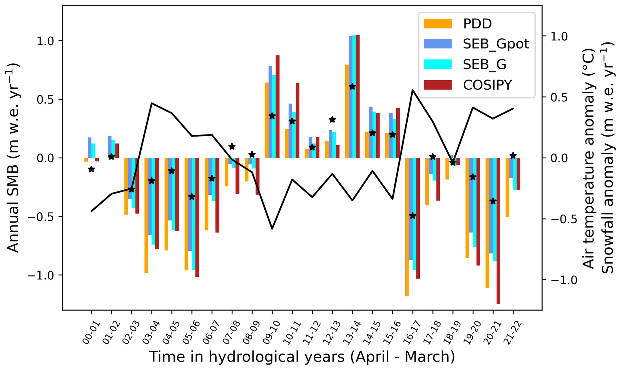
Figure 6Annual massif-wide average SMB for the four SMB models (left axis) together with the anomaly of temperature (black line) and snowfall (black star) from the 2000–2022 average (right axis).
4.3 Model intercomparison
We can compare modeled and observed MB for the individual glacier catchments to assess the performance of the individual models (Fig. 7). The area-weighted RMSE (Table 2) is similar for the PDD, SEB_Gpot and SEB_G (0.17, 0.19 and 0.16 m w.e. yr−1) and largest for COSIPY (0.31 m w.e. yr−1) comparing land-terminating glaciers. The range of uncertainty of the RMSEs is very similar for all four models (see Table S6), with RMSEs lying between 0.16 and 0.34 m w.e. yr−1. Only the PDD stands out, with a maximum RMSE of 0.75 m w.e. yr−1. The BMSMnc range of the 10 best-ranked runs are very similar (range below 0.24 m w.e. yr−1) for the SEB_Gpot, SEB_G and COSIPY. For the PDD, this range is distinctly larger with 0.51 m w.e. yr−1 taking the five (due to the smaller sample size) best-ranked runs.
In order to investigate the importance of including accurate information about incoming radiation, we can directly compare the performance of the SEB_Gpot with the SEB_G. The former relies on the potential radiation, whereas the latter accurately calculates the direct and diffuse parts of incoming shortwave radiation by taking into account cloud cover and shading. Generally, both models tend to overestimate the SMB in the MSM (Fig. 7), which is also reflected in the overestimation of the BMSMnc (−0.33 and −0.32 m w.e. yr−1 for the SEB_Gpot and SEB_G, respectively) (Table 2). The differences between both models are overall minor, although the RMSE for the SEB_G is smaller (Table 2). Thus, for this study site, the improvement by using more accurate instead of potential radiation appears insignificant. This finding further agrees with the fact that the PDD also produces satisfying results.
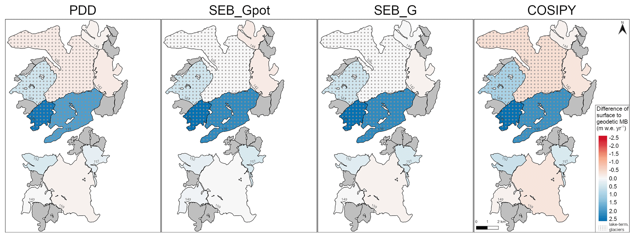
Figure 7Difference of modeled surface to observed geodetic MB (2000–2013) for the four SMB models. Dotted areas indicate lake termination precluding a direct comparison of the two data sets. The displayed results for the PDD are those from Strategy C in Fig. 3. Grey shading indicates glaciers with an area <3 km2. Glacier outlines mark the 2004 extent.
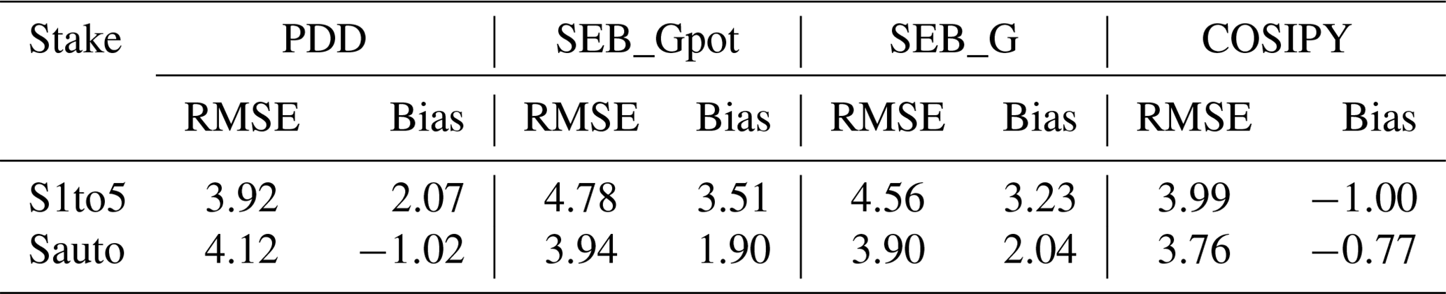
The second observation available for model evaluation is the stake measurements. However, the agreement between measured and modeled ablation at the stakes is poor for all considered SMB models (see Fig. S4 and S5). Mean RMSEs are in the range between 3.92 and 4.78 m w.e. yr−1 (Table 3), which is about 33 % of the observed melt. The model bias ranges between −0.77 and 3.51 m w.e. yr−1. The best results are achieved with COSIPY, followed by the PDD regarding both RMSE and bias. At the individual ablation stakes (Fig. S4), COSIPY behaves distinctly differently from the other models, for which melt rates are more similar most of the time. Subsequently, COSIPY meets the observations better for the first half of the time when the other models underestimate the melting. However, after 2018, COSIPY clearly overestimates the melt rates degrading the overall statistics. In general, we consider the ablation measurements to be error-prone when looking at individual observations. Thus, we consider the large RMSE and bias values to be caused only partly by poor model performance.
Table 3Comparison (RMSE and mean bias; m w.e. yr−1) between observed and modeled melt at the stakes. S1to5 includes all individual stake observations in 2013–2019, and Sauto comprises the measurements by the automatic ablation sensor.
5.1 Strategies for model calibration
The single-glacier model calibration at Schiaparelli Glacier (Strategy A) results in a TLR of −0.70 ∘C 100 m−1, which is slightly stronger compared to previously reported annual values that vary from −0.60 to −0.67 ∘C 100 m−1 in the southern Patagonian region (Strelin and Iturraspe, 2007; Buttstädt et al., 2009; Koppes et al., 2009; Schaefer et al., 2015; Weidemann et al., 2018a, 2020). Furthermore, calibration suggests a τ of 850 s, which differs significantly from the value used at Schiaparelli Glacier in a recent SMB study (Weidemann et al., 2020). However, it agrees well with values reported in various other applications, including southern Patagonia (Smith and Barstad, 2004; Barstad and Smith, 2005; Smith and Evans, 2007; Schuler et al., 2008; Jarosch et al., 2012; Sauter, 2020). The degree-day factors DDFice and DDFsnow of 6.0 and 3.0 mm d−1 ∘C−1, respectively, lie within the range of previously reported values (Stuefer et al., 2007; Gabbi et al., 2014; Réveillet et al., 2017). At Gran Campo Nevado, Schneider et al. (2007) found a value of 7.6 mm d−1 ∘C−1 for ice in summertime. Calculating the average DDFice directly from measured ablation and a positive degree-day sum at the stake locations (Groos et al., 2017) delivers values very close to the calibrated one, with 5.0 mm d−1 ∘C−1 at the automatic ablation sensor and 6.0 mm d−1 ∘C−1 at the individual stakes.
Going from a single-glacier calibration (Strategy A) to a regional calibration (Strategy B), the TLR and τ need changing, and the DDFice decreases slightly to 5.0 mm d−1 ∘C−1. A TLR of −0.60 ∘C 100 m−1 is required, which is distinctly lower than the result of Strategy A. However, this value is close to values used in the Cordillera Darwin before ranging from −0.60 to −0.63 ∘C 100 m−1 (Strelin and Iturraspe, 2007; Koppes et al., 2009). The τ of 1200 s produces a precipitation field with less orographic contribution compared to Strategy A. The value is still distinctly smaller than in Weidemann et al. (2020). Both changes significantly reduce the snowfall amounts and result in a better match with observed geodetic MBs.
The results suggest that the exclusive use of ablation stakes (Weidemann et al., 2020), which have been installed in the lowest part of Schiaparelli Glacier, for model calibration shows limited utility because no information about accumulation is included. Thus, adding the total mass budget of Schiaparelli Glacier by a flux gate approach brings significant benefit to constrain the drainage basin-wide mass input. Still, the transfer of a SMB model, which has been calibrated to a single glacier, to a regional study site (Strategy A) can imply severe biases in the overall mass budget. This demonstrates that model parameters are not transferable from one single glacier to the surroundings. This shortcoming has been reported similarly in previous studies with various melt models and at many locations (e.g., MacDougall and Flowers, 2011; Gurgiser et al., 2013; Zolles et al., 2019). In general, the SMB in the MSM is excessively overestimated, which indicates that the SMB model either produces too little melt or receives excessive snowfall. The latter seems more likely, since melt is well constrained by the stake measurements at least at Schiaparelli Glacier, whereas the precipitation amounts are generally more uncertain. By the use of a regional calibration strategy (Strategy B), the agreement between the observed geodetic and modeled surface MB can be significantly improved. This highlights the importance of including regional observations for realistic simulations of regional surface mass balance in the Cordillera Darwin.
Considering the regional distribution of the difference of SMB from the geodetic observations (Fig. 4), the model tends to overestimate the MB on the land-terminating glaciers in the northwest (e.g., 149, 152) and underestimate it in the southeast (e.g., Emma, Pagels) of the massifs. This pattern indicates that snowfall amounts are overestimated on the northwestern slopes and underestimated on the southeastern slopes, which may be associated with the neglect of climatic gradients, e.g., in temperature or precipitation. Mass transfer by snowdrift due to the consistent westerlies has been neglected so far. With the addition of a basic snowdrift scheme (Strategy C), the agreement between modeled and observed mass balance can be improved further. Thus, the results show that snowdrift plays an important role for the SMB in the MSM.
The calibration of the SEB models and COSIPY reveals realistic parameter values within the range of previous applications as well (see Table 1). For COSIPY, the calibrated parameters zice and αfirn lie on the margin of the range, implying that a larger range may be beneficial or that a parameter not considered in calibration is not chosen optimally. However, extending the limits of these parameters would result in physically unrealistic values. We have not been able to find a parameter that was neglected in the calibration and that would solve the issue. Apart from the model-inherent parameters, the difficulties with the calibration of COSIPY might alternatively lie in the input data set. Variables that are only considered in COSIPY and not in the other models are, e.g., wind speed and relative humidity, which both affect turbulent heat fluxes and thereby impact the choice of ice roughness length.
A high discrepancy between modeled and observed mass balance is obtained for two lake-terminating glaciers south of Monte Sarmiento (138 and Lovisato) (Fig. 7). Due to the lake termination, it is expected that the modeled SMB will be higher than the geodetic MB. However, the difference is extremely large, especially when considering snow redistribution due to snowdrift. In Sect. 5.4, we will discuss possible explanations for this discrepancy.
5.2 Surface mass balance of the Monte Sarmiento Massif
The mean annual SMB of −0.79 to −1.20 m w.e. yr−1 (2000–2013) at Schiaparelli Glacier is distinctly less negative than the previous estimate for the period 2000–2017 ( m w.e. yr−1) by Weidemann et al. (2020) but in much better agreement with the satellite observations ( m w.e. yr−1). The massif-wide average SMB over the full study period (2000–2022) is estimated between −0.28 and −0.07 m w.e. yr−1 depending on the model choice. In the eastern part of the CDI, an average SMB of −0.53 m w.e. yr−1 was simulated between 2000 and 2006 using a PDD model (Buttstädt et al., 2009). Similarly large accumulation amounts over the highest parts of the glaciers and the extreme ablation over the glacier tongues, which we see at our study site, have been reported for the Southern Patagonian Icefield (Schaefer et al., 2015). We can confirm that the SMB of the MSM is controlled by winter accumulation and summer temperature, as has been observed in the Cordillera Darwin before (Weidemann et al., 2020; Mutz and Aschauer, 2022). The orientation of the individual glaciers does not seem to dictate a particular pattern. Glaciers that receive more direct solar radiation (e.g., Schiaparelli, Conway, Pagels) do not show more negative MBs than glaciers with stronger shading (e.g., Lovisato, 138).
We simulate an average equilibrium-line altitude (ELA) at 770–795 m for the MSM. This is close to the mean ELA at 730 ± 50 m simulated at Schiaparelli Glacier in 2000–2017 (Weidemann et al., 2020) but higher than the ELA suggested by Bown et al. (2014) for Ventisquero Glacier at the southwestern edge of the CDI at around 650 m in 2004. At the CDI's northern edge at Marinelli Glacier and the eastern edge at Martial Este Glacier, average ELAs have been reported at around 1100 m (Buttstädt et al., 2009; Bown et al., 2014). The altitude difference can be explained by the more continental conditions due to leeside effects that reduce the precipitation in the east of the CDI (Strelin and Iturraspe, 2007), while the MSM is located at the western edge of the CDI, directly exposed to the moist westerly winds causing abundant precipitation and, thus, higher accumulation amounts (Bown et al., 2014), which results in lower equilibrium lines.
Ice losses due to dynamical adjustment and calving are assumed to play an important role only for a few glaciers in the CDI (Koppes et al., 2009; Bown et al., 2014; Weidemann et al., 2020), like Marinelli Glacier (Porter and Santana, 2003). Weidemann et al. (2020) conclude that mass loss due to SMB processes is the main reason for the recent areal changes of Schiaparelli Glacier. Based on our results, we can confirm that the SMB contributes the largest amount to the ice loss at Schiaparelli Glacier. However, calving is not negligible. Using calibration Strategy A, where the PDD model is tuned to the Schiaparelli Glacier conditions directly, we assess a resulting calving flux of 0.17 m w.e. yr−1, which equals a mass loss of 4.26 Mt yr−1 at Schiaparelli Glacier. The average geodetic MB estimated from elevation changes for the whole study site is with −0.55 m w.e. yr−1 (2000–2013) distinctly more negative than the SMB (−0.28 m w.e. yr−1 by the PDD, in the same period), indicating that calving losses are not insignificant in the region. However, in order to determine the calving flux more accurately, detailed information about the ice thickness and velocities at the glacier fronts is required.
5.3 Model intercomparison
Overall, we achieve a very good agreement between the modeled surface and the observed geodetic MB. For most glaciers, the RMSEs are in a similar range to the uncertainties in geodetic MB (Table S5). We want to highlight the remarkable performance of all four models used under these challenging conditions, with very sparse observations leading to overparameterization issues.
Previous studies (e.g., Six et al., 2009; Gabbi et al., 2014; Réveillet et al., 2017) of melt model comparison have come to the conclusion that more complex, physically based models can achieve more realistic SMB results in case they are based on high-quality and well-distributed in situ observations. If observations are limited or inferred from distant weather stations, the performance decreases rapidly, and less complex, empirical models produce better results (Gabbi et al., 2014; Réveillet et al., 2017). Since we focus on a study area where in situ measurements are extremely limited and, thus, need to infer model input from reanalysis data via downscaling, and furthermore glacier SMB is known to be highly correlated with precipitation and air temperature (Weidemann et al., 2020), we strongly challenge the question of which SMB model can produce the most realistic SMB.
Results are validated against the individual geodetic MBs and the stake measurements. The results of this study show that less complex model types overall outperform COSIPY, although the simulated melt at the ablation stakes is best represented by COSIPY. Both SEB model variants tend to overestimate the SMB in the MSM on average, but the SEB_G achieves the smallest RMSE compared to geodetic observations of the land-terminating glaciers. The MB of Schiaparelli Glacier, the largest glacier of the massif, is also simulated well by both SEB variants. Comparison of the measured against modeled melt at the stakes delivers similar results for all the models with large RMSEs (Table 3). Although COSIPY achieves the overall smallest RMSE and bias, the difference from the other models is small compared to the difference from the measurements.
Gabbi et al. (2014) concluded that models considering the temperature- and radiation-induced melt separately are more suitable for long-term simulation periods because they are less sensitive to temperature. However, shorter time periods might not be able to bring issues like parameter instability to light (Gabbi et al., 2014), which might apply to our study period. The importance of correct radiation information cannot be confirmed even by comparing the two SEB model variants we used. Although the agreement with observations can be increased (see Table S1), including accurate radiation calculation (SEB_G) instead of potential radiation (SEB_Gpot) only produces a minor improvement in the glacier-wide SMBs. Interestingly, the SEB_G always produces slightly larger melt rates at the individual stake locations (Fig. S4), whereas at the automatic ablation sensor we do not see this consistent pattern (Fig. S5).
Overall, due to the small sample size of glaciers, it is not possible to point out the one best-suited SMB model for the MSM. The strong correlation with air temperature and precipitation makes the PDD a good predictor of the SMB. Both SEB model variants show a convincing performance as well, although they tend to produce a less negative BMSMnc. Still, the highest agreement with geodetic MB is achieved using the SEB_G. COSIPY delivers more accurate and confident results (smaller uncertainty) (Table S6) and can best reproduce the melt at the stakes. As in this study, in Schneider et al. (2007) the applied PDD and energy balance model at the Gran Campo Nevado showed very similar results. In order to better understand the interaction between the atmosphere and the glacier surface, a physically based energy and mass balance model like COSIPY is advantageous.
5.4 Challenges and limitations
A large discrepancy between the surface and geodetic MB is modeled for glaciers 138 and Lovisato. Both glaciers are calving: thus, a positive anomaly in SMB is to be expected, but the difference seems very high. Including the snowdrift parameterization (Strategy C), the discrepancy gets even larger due to the mainly prevailing northwesterlies during snowfall events. The results from the four different SMB models imply a mass loss through calving of 2.5 to 2.9 m w.e. yr−1 and 1.9 to 2.2 m w.e. yr−1 for glaciers 138 and Lovisato, which equals ice masses of 9.73 to 11.28 Mt yr−1 and 23.88 to 27.65 Mt yr−1, respectively. We will discuss in the following whether these values are realistic.
Assessing satellite images of the last few years, it can be confirmed that Lovisato Glacier has significant calving losses, seen through large numbers of icebergs in the proglacial lake (see Fig. 1). Lovisato Glacier has a frontal width of around 500 m. Satellite observations suggest surface velocities of around 400 m yr−1 in recent years. In order to obtain the suggested ice mass loss of 23.88 to 27.65 Mt yr−1, an ice thickness of around 130–150 m would be necessary. The 2019 consensus estimate gives an ice thickness of up to ∼190 m in this area of Lovisato Glacier (Farinotti et al., 2019). Other ice thickness reconstructions estimate a thickness between 144 and 200 m (Carrivick et al., 2016; Millan et al., 2022). Subsequently, the high calving rates suggested by our results are realistic for Lovisato Glacier.
For glacier 138, however, we do not see any major icebergs that would indicate a significant calving flux. Surface velocities are below 20 m yr−1 and maximum ice thickness between 50 and 70 m (Farinotti et al., 2019; Millan et al., 2022). This would result in calving flux magnitudes smaller than implied by our results. Therefore, we reject the calving explanation for glacier 138. It is one of the smallest glaciers that we included in the comparison with satellite observations. Due to the small size, the uncertainty in the observed elevation change rate is large. Furthermore, the DEMs used for the calculations have large gaps over this glacier, specifically in the accumulation area. Thus, we assume that in reality the uncertainty for glacier 138 is even larger, which could cause the large difference between model and observation in this case.
Other factors that could explain the large discrepancy between geodetic and surface MB are limitations in the snowdrift parameterization. The snowdrift scheme does not track the snow on its way from one location to another but identifies locations sheltered from or exposed to wind and, subsequently, corrects the snowfall amounts based on that. Looking at the study site, the question can be asked where the snow deposited at glacier 138 should come from. The main snowdrift direction is towards the southeast. There is no area directly northwest of glacier 138, where we would expect much snowfall that could be blown to and deposited at glacier 138. This highlights one limitation of the snowdrift parameterization. However, even without snowdrift (Strategy B), our results require a calving flux of more than 1.42 m w.e. yr−1 (Table 2). Thus, limitations are given by the SMB model itself and the climatic forcing as well.
Using one TLR throughout the whole study site and throughout the year is a major simplification. SMB models are highly sensitive to the air temperature field. It is known that the TLR over mountainous terrain varies not only temporally, but also locally (Gardner and Sharp, 2009; Gardner et al., 2009; Petersen et al., 2013; Ayala et al., 2015; Heynen et al., 2016; Shaw et al., 2016; Shen et al., 2016; Hanna et al., 2017). Bravo et al. (2019a) found that the observed lapse rates at the SPI are steeper in the east compared to the west and that differences exist between the lower and upper sections of glaciers. Thus, it is possible that a northwest-to-southeast gradient in temperature (lapse rate) prevails in the MSM, affecting the SMB. However, since we do not have any measurements of TLR at the study site that would allow a more realistic estimate, a constant and linear lapse rate is applied.
We investigated strategies for SMB model calibration in the Cordillera Darwin in order to achieve realistic simulations of the regional SMB. Therefore, we applied three different calibration strategies, ranging from a local single-glacier calibration transferred to the regional scale (Strategy A) to a regional calibration without (Strategy B) and with (Strategy C) the inclusion of a snowdrift parameterization. In this way, we examined the model transferability in space, the advantage of regional mass change observations and the benefit of increasing the complexity level regarding included processes. Furthermore, we constrained the main characteristics of SMB in the MSM. We considered the following measurements: ablation and ice thickness measurements at Schiaparelli Glacier as well as elevation changes and flow velocities from satellite data for the entire study site. Performance of simulated MB is validated against geodetic mass changes and stake observations.
Our analysis suggests that the exclusive use of ablation stakes from the lowest part of Schiaparelli Glacier for model calibration shows limited utility because no information about accumulation is included. Adding the total mass budget of Schiaparelli Glacier by a flux gate approach brings significant benefit to constrain the drainage basin-wide mass input. Still, calibration at one single glacier and subsequent transfer to regional scales (Strategy A) resulted in a clearly biased SMB. Such an important bias implies that spatial model transfers are critical even on such small scales as the MSM. Model performance can be significantly improved by the use of remotely sensed regional observations (Strategy B), e.g., the annual massif-wide average geodetic MB. Such observations are available on global scales, often dating back to 2000 (e.g., Hugonnet et al., 2021). Including a snowdrift parameterization (Strategy C) can further increase the agreement between modeled and observed MB of individual glacier basins. This demonstrates that snowdrift has an important influence on the accumulation in the MSM, where strong and consistent westerly winds prevail.
To answer the main study questions, we can summarize that this study has shown that transferring SMB models in space is a challenge, and common practices can produce distinctly biased estimates (Q1). Thus, we advise incorporating regional observations for a regional application of SMB models (Q2). Furthermore, we have shown that snowdrift does play an important role for the SMB in the Cordillera Darwin, and thus the inclusion of this process is beneficial (Q3). However, increasing the complexity level of the SMB models from an empirical approach to a physically based model did not result in an improvement. The main characteristics of SMB in the MSM are reproduced in a similar way by all four models applied in this study. The massif-wide average annual SMB between 2000 and 2022 ranges between −0.28 and −0.07 m w.e. yr−1 with an average ELA between 770 and 795 m, depending on the exact model. The SMB is mainly controlled by melt and snowfall, as has been observed similarly in southern Patagonia. The spatial pattern is characterized by high amounts of snowfall over the high-altitude areas up to 10 m w.e. yr−1 and extreme surface melt over the glacier tongues down to −10 m w.e. yr−1. The model intercomparison did not indicate one clear best-suited model for SMB simulations in the MSM. Thus, the performance of the SMB cannot generally be improved by increasing the complexity level of the model. The PDD delivered unexpectedly good results considering the simplicity of the model. However, the physically based model COSIPY, which is much more challenging to calibrate, did produce convincing results as well and might produce slightly more stable values (smaller uncertainty and range of values in the 10 top-ranked simulations). Both SEB model variants show reasonable results as well, although they tend to overestimate the average SMB in the MSM. Overall, the SEB_G achieves the best agreement with geodetic observations.
The main limitations of this study are the sparse observations in the Cordillera Darwin, which cause overparameterization and preclude extensive model calibration and validation. We particularly missed information about precipitation amounts in mountainous areas. Moreover, measurements of TLR are missing, which we have shown to be essential for the SMB simulations. With the combination of in situ and satellite observations, we have been able to appropriately calibrate both fields. However, the uncertainties linked to the climatic forcing are still large. Including snowdrift and solely considering regional calibration targets together with mass budgeting of the most prominent Schiaparelli Glacier, we succeeded in reducing the RMSE with respect to the geodetic measurements to their associated errors.
ERA5 reanalysis data are available via the Copernicus Climate Data Store (https://doi.org/10.24381/cds.adbb2d47, Hersbach et al., 2023a; https://doi.org/10.24381/cds.bd0915c6, Hersbach et al., 2023b). Ice thickness measurements in 2016 are accessible at https://doi.org/10.1594/PANGAEA.919331 (Gacitúa et al., 2020). Meteorological and ablation stake observations are freely available on the Pangaea Database: AWS Rock (https://doi.org/10.1594/PANGAEA.956569, Schneider et al., 2023), AWS Glacier (https://doi.org/10.1594/PANGAEA.958694, Arginoy-Neto et al., 2023), ablation stakes (https://doi.org/10.1594/PANGAEA.958668, Jaña et al., 2023) and ablation sensor (https://doi.org/10.1594/PANGAEA.958623, Netto et al., 2023). The code for the COSIPY model (version 1.4) is available at https://github.com/cryotools/cosipy (last acccess: 7 June 2023) (https://doi.org/10.5281/zenodo.4439551, Arndt et al., 2021b). The code for the PDD model is available at https://doi.org/10.5281/zenodo.8009967 (Temme, 2023a). The code for the two SEB model variants is available at https://doi.org/10.5281/zenodo.8009978 (Temme, 2023b). Model forcing and SMB model output of this study are available at https://doi.org/10.5281/zenodo.7798666 (Temme et al., 2023).
The supplement related to this article is available online at: https://doi.org/10.5194/tc-17-2343-2023-supplement.
The concept of this study was developed by JJF, FT and CS. FT implemented the simulations with the support of TS, AA and JJF. In situ observational data were collected and provided by CS, RJ, JAN and IG. Satellite observations were processed and provided by DFB and TS. FT led the writing process with the support of all the authors.
The contact author has declared that none of the authors has any competing interests.
The presented content only reflects the authors' views, and the European Research Council Executive Agency is not responsible for
any use that may be made of the information it contains.
Publisher’s note: Copernicus Publications remains neutral with regard to jurisdictional claims in published maps and institutional affiliations.
The authors want to thank Thomas Mölg, who provided the model code for the radiation module. The authors are grateful for the scientific support and resources provided by the Erlangen National High Performance Computing (HPC) Center (NHR@FAU) of the Friedrich-Alexander-Universität Erlangen-Nürnberg (FAU). NHR funding is provided by federal and Bavarian state authorities. NHR@FAU hardware is partially funded by the DFG – 440719683. The authors want to thank the Chilean National Forest Corporation (CONAF) for enabling and supporting the field work in the Monte Sarmiento Massif, Parque Nacional Alberto de Agostini.
This research was funded by the German Research Foundation (DFG) within the MAGIC project (FU 1032/5-1). Fürst has received funding from the European Union’s Horizon 2020 research and innovation programme via the European Research Council (ERC) as a Starting Grant (StG) under grant agreement No 948290. Farías-Barahona was funded by the DFG within the MAGIC and ITERATE projects (FU1032/5-1, BR2105/28-1, FU1032/12-1) as well as by ANID Subvención a la instalación a la academia 2022 (PAI85220007), and Anillo ACT210080. Seehaus received support by the ESA Living Planet Fellowship Programme (Project MIT-AP). Arigony-Neto received funding from the Rio Grande do Sul state Research Support Foundastion (FAPERGS nos. 17/25510000518-0 and 21/2551-0002034-2).
This paper was edited by Valentina Radic and reviewed by David Rounce and Enrico Mattea.
Albrecht, T., Winkelmann, R., and Levermann, A.: Glacial-cycle simulations of the Antarctic Ice Sheet with the Parallel Ice Sheet Model (PISM) – Part 2: Parameter ensemble analysis, The Cryosphere, 14, 633–656, https://doi.org/10.5194/tc-14-633-2020, 2020.
Arigony-Neto, J., Jaña, R., Gonzalez, Inti, Schneider, C., and Temme, F.: Meteorological Observations at Schiaparelli Glacier Automatic Weather Station (AWSglacier), Cordillera Darwin, Chile, 2013–2019, PANGAEA [data set], https://doi.org/10.1594/PANGAEA.958694, 2023.
Arndt, A., Scherer, D., and Schneider, C.: Atmosphere Driven Mass-Balance Sensitivity of Halji Glacier, Himalayas, Atmosphere, 12, 426, https://doi.org/10.3390/atmos12040426, 2021a.
Arndt, A., Sauter, T., and Saß, B.: COSIPY v1.4, Zenodo [code], https://doi.org/10.5281/zenodo.4439551, 2021b.
Ayala, A., Pellicciotti, F., and Shea, J. M.: Modeling 2 m air temperatures over mountain glaciers: Exploring the influence of katabatic cooling and external warming, J. Geophys. Res.-Atmos., 120, 3139–3157, https://doi.org/10.1002/2015JD023137, 2015.
Barandun, M., Pohl, E., Naegeli, K., McNabb, R., Huss, M., Berthier, E., Saks, T., and Heolzle, M.: Hot spots of glacier mass balance variability in Central Asia, Geophys. Res. Lett., 48, e2020GL092084, https://doi.org/10.1029/2020GL092084, 2021.
Barcaza, G., Nussbaumer, S. U., Tapia, G., Valdés, J., García, J. L., Videla, Y., Albornoz, A., and Arias, V.: Glacier inventory and recent glacier variations in the Andes of Chile, South America, Ann. Glaciol., 58, 166–180, https://doi.org/10.1017/aog.2017.28, 2017.
Barstad, I. and Smith, R. B.: Evaluation of an orographic precipitation model, J. Hydrometeorol., 6, 85–99, https://doi.org/10.1175/JHM-404.1, 2005.
Bentley, C. R.: Mass balance of the Antarctic ice sheet: observational aspects, in: Mass Balance of the Cryosphere, Observations and Modelling of Contemporary and Future Changes, edited by: Houghton, J., Bamber, J., and Payne, A., Cambridge University Press, Cambridge, 459–490, https://doi.org/10.1017/cbo9780511535659.014, 2009.
Bown, F., Rivera, A., Zenteno, P., Bravo, C., and Cawkwell, F.: First Glacier Inventory and Recent Glacier Variation on Isla Grande de Tierra Del Fuego and Adjacent Islands in Southern Chile, in: Global Land Ice Measurements from Space, edited by: Kargel, J., Leonard, G., Bishop, M., Kääb, A., and Raup, B., Springer, Berlin, Heidelberg, 661–674, https://doi.org/10.1007/978-3-540-79818-7_28, 2014.
Bown, F., Rivera, A., Peȩtlicki, M., Bravo, C., Oberreuter, J., and Moffat, C.: Recent ice dynamics and mass balance of Jorge Montt Glacier, Southern Patagonia Icefield, J. Glaciol., 65, 732–744, https://doi.org/10.1017/jog.2019.47, 2019.
Braithwaite, R.: Positive degree-day factors for ablation on the Greenland ice sheet studied by energy-balance modelling, J. Glaciol., 41, 153–160, https://doi.org/10.3189/S0022143000017846, 1995.
Braun, M. H., Malz, P., Sommer, C., Farías-Barahona, D., Sauter, T., Casassa, G., Soruco, A., Skvarca, P., and Seehaus, T. C.: Constraining glacier elevation and mass changes in South America, Nat. Clim. Change, 9, 130–136, https://doi.org/10.1038/s41558-018-0375-7, 2019.
Bravo, C., Quincey, D. J., Ross, A. N., Rivera, A., Brock, B., Miles, E., and Silva, A.: Air Temperature Characteristics, Distribution, and Impact on Modeled Ablation for the South Patagonia Icefield, J. Geophys. Res.-Atmos., 124, 907–925, https://doi.org/10.1029/2018JD028857, 2019a.
Bravo, C., Bozkurt, D., Gonzalez-Reyes, Á., Quincey, D. J., Ross, A. N., Farías-Barahona, D., and Rojas, M.: Assessing snow accumulation patterns and changes on the Patagonian Icefields, Front. Environ. Sci., 7, 1–18, https://doi.org/10.3389/fenvs.2019.00030, 2019b.
Brock, B., Willis, I., and Sharp, M.: Measurement and parameterization of aerodynamic roughness length variations at Haut Glacier d’Arolla, Switzerland, J. Glaciol., 52, 281–297, https://doi.org/10.3189/172756506781828746, 2006.
Buisán, S. T., Earle, M. E., Collado, J. L., Kochendorfer, J., Alastrué, J., Wolff, M., Smith, C. D., and López-Moreno, J. I.: Assessment of snowfall accumulation underestimation by tipping bucket gauges in the Spanish operational network, Atmos. Meas. Tech., 10, 1079–1091, https://doi.org/10.5194/amt-10-1079-2017, 2017.
Buttstädt, M., Möller, M., Iturraspe, R., and Schneider, C.: Mass balance evolution of Martial Este Glacier, Tierra del Fuego (Argentina) for the period 1960–2099, Adv. Geosci., 22, 117–124, https://doi.org/10.5194/adgeo-22-117-2009, 2009.
Cannon, A. J., Sobie, S. R., and Murdock, T. Q.: Bias correction of GCM precipitation by quantile mapping: How well do methods preserve changes in quantiles and extremes?, J. Climate, 28, 6938–6959, https://doi.org/10.1175/JCLI-D-14-00754.1, 2015.
Carrivick, J. L., Davies, B. J., James, W. H. M., Quincey, D. J., and Glasser, N. F.: Distributed ice thickness and glacier volume in southern South America, Global Planet. Change, 146, 122–132, https://doi.org/10.1016/j.gloplacha.2016.09.010, 2016.
Cogley, J. C., Rasmussen, L. A., Arendt, A. A., Bauder, A., Braithwaite, R. J., Jansson, P., Kaser, G., Möller, M., Nicholson, M., and Zemp, M.: Glossary of Glacier Mass Balance and Related Terms, IACS Contrib. No. 2, 2011.
Cullen, N., Mölg, T., Kaser, G., Steffen, K., and Hardy, D.: Energy-balance model validation on the top of Kilimanjaro, Tanzania, using eddy covariance data, Ann. Glaciol., 46, 227–233, https://doi.org/10.3189/172756407782871224, 2007.
Dadic, R., Mott, R., Lehning, M., and Burlando, P.: Parameterization for wind-induced preferential deposition of snow, Hydrol. Process., 24, 1994–2006, https://doi.org/10.1002/hyp.7776, 2010.
DGA: Metodología de inventario público de glaciares, SDT No. 447, 2022. Ministerio de Obras Públicas, Dirección General de Aguas Unidad de Glaciología y Nieves, realizado por: Casassa, G., Espinoza, A., Segovia, A., and Huenante, J., 2022.
Dussaillant, I., Berthier, E., Brun, F., Masiokas, M., Hugonnet, R., Favier, V., Rabatel, A., Pitte, P., and Ruiz, L.: Two decades of glacier mass loss along the Andes, Nat. Geosci., 12, 802–808, https://doi.org/10.1038/s41561-019-0432-5, 2019.
Farinotti, D., Huss, M., Fürst, J. J., Landmann, J., Machguth, H., Maussion, F., and Pandit, A.: A consensus estimate for the ice thickness distribution of all glaciers on Earth, Nat. Geosci., 12, 168–173, https://doi.org/10.1038/s41561-019-0300-3, 2019.
Gabbi, J., Carenzo, M., Pellicciotti, F., Bauder, A., and Funk, M.: A comparison of empirical and physically based glacier surface melt models for long-term simulations of glacier response, J. Glaciol., 60, 1199–1207, https://doi.org/10.3189/2014JoG14J011, 2014.
Gacitúa, G., Schneider, C., and Casassa, G.: Ice thickness observations in Glacier Schiaparelli, Cordillera Darwin, Chile, PANGAEA [data set], https://doi.org/10.1594/PANGAEA.919331, 2020.
Gacitúa, G., Schneider, C., Arigony, J., González, I., Jaña, R., and Casassa, G.: First ice thickness measurements in Tierra del Fuego at Schiaparelli Glacier, Chile, Earth Syst. Sci. Data, 13, 231–236, https://doi.org/10.5194/essd-13-231-2021, 2021.
Gardner, A. S. and Sharp, M.: Sensitivity of net mass-balance estimates to near-surface temperature lapse rates when employing the degree-day method to estimate glacier melt, Ann. Glaciol., 50, 80–86, https://doi.org/10.3189/172756409787769663, 2009.
Gardner, A. S., Sharp, M. J., Koerner, R. M., Labine, C., Boon, S., Marshall, S. J., Burgess, D. O., and Lewis, D.: Near-surface temperature lapse rates over arctic glaciers and their implications for temperature downscaling, J. Climate, 22, 4281–4298, https://doi.org/10.1175/2009JCLI2845.1, 2009.
Garreaud, R. D., Vuille, M., Compagnucci, R., and Marengo, J.: Present-day South American climate, Palaeogeogr. Palaeocl., 281, 180–195, https://doi.org/10.1016/j.palaeo.2007.10.032, 2009.
Glasser, N. F., Harrison, S., Winchester, V., and Aniya, M.: Late Pleistocene and Holocene palaeoclimate and glacier fluctuations in Patagonia, Global Planet. Change, 43, 79–101, https://doi.org/10.1016/j.gloplacha.2004.03.002, 2004.
Groos, A. R., Mayer, C., Smiraglia, C., Diolaiuti, G., and Lambrecht, A.: A first attempt to model region-wide glacier surface mass balances in the Karakoram: Findings and future challenges, Geogr. Fis. Din. Quat., 40, 137–159, https://doi.org/10.4461/GFDQ.2017.40.10, 2017.
Gudmundsson, L., Bremnes, J. B., Haugen, J. E., and Engen-Skaugen, T.: Technical Note: Downscaling RCM precipitation to the station scale using statistical transformations – a comparison of methods, Hydrol. Earth Syst. Sci., 16, 3383–3390, https://doi.org/10.5194/hess-16-3383-2012, 2012.
Gurgiser, W., Molg, T., Nicholson, L., and Kaser, G.: Mass-balance model parameter transferability on a tropical glacier, J. Glaciol., 59, 845–858, https://doi.org/10.3189/2013JoG12J226, 2013.
Hanna, E., Mernild, S., de Villiers, S., and Yde, J.: Surface air temperature variations and lapse rates on Olivares Gamma Glacier, Rio Olivares Basin, Central Chile, from a novel meteorological sensor network, Meteorol. Appl., 2017, 12–14, 2017.
Hersbach, H., Bell, B., Berrisford, P., Hirahara, S., Horányi, A., Muñoz-Sabater, J., Nicolas, J., Peubey, C., Radu, R., Schepers, D., Simmons, A., Soci, C., Abdalla, S., Abellan, X., Balsamo, G., Bechtold, P., Biavati, G., Bidlot, J., Bonavita, M., de Chiara, G., Dahlgren, P., Dee, D., Diamantakis, M., Dragani, R., Flemming, J., Forbes, R., Fuentes, M., Geer, A., Haimberger, L., Healy, S., Hogan, R. J., Hólm, E., Janisková, M., Keeley, S., Laloyaux, P., Lopez, P., Lupu, C., Radnoti, G., de Rosnay, P., Rozum, I., Vamborg, F., Villaume, S., and Thépaut, J. N.: The ERA5 global reanalysis, Q. J. Roy. Meteor. Soc., 146, 1999–2049, https://doi.org/10.1002/qj.3803, 2020.
Hersbach, H., Bell, B., Berrisford, P., Biavati, G., Horányi, A., Muñoz Sabater, J., Nicolas, J., Peubey, C., Radu, R., Rozum, I., Schepers, D., Simmons, A., Soci, C., Dee, D., and Thépaut, J. N.: ERA5 hourly data on single levels from 1940 to present, Copernicus Climate Change Service (C3S) Climate Data Store (CDS) [data set], https://doi.org/10.24381/cds.adbb2d47, 2023a.
Hersbach, H., Bell, B., Berrisford, P., Biavati, G., Horányi, A., Muñoz Sabater, J., Nicolas, J., Peubey, C., Radu, R., Rozum, I., Schepers, D., Simmons, A., Soci, C., Dee, D., and Thépaut, J. N.: ERA5 hourly data on pressure levels from 1940 to present, Copernicus Climate Change Service (C3S) Climate Data Store (CDS) [data set], https://doi.org/10.24381/cds.bd0915c6, 2023b.
Heynen, M., Miles, E., Ragettli, S., Buri, P., Immerzeel, W. W., and Pellicciotti, F.: Air temperature variability in a high-elevation Himalayan catchment, Ann. Glaciol., 57, 212–222, https://doi.org/10.3189/2016AoG71A076, 2016.
Hock, R.: A distributed temperature-index ice- and snowmelt model including potential direct solar radiation, J. Glaciol., 45, 101–111, 1999.
Hugonnet, R., McNabb, R., Berthier, E., Menounos, B., Nuth, C., Girod, L., Farinotti, D., Huss, M., Dussaillant, I., Brun, F., and Kääb, A.: Accelerated global glacier mass loss in the early twenty-first century, Nature, 592, 726–731, https://doi.org/10.1038/s41586-021-03436-z, 2021.
Huintjes, E., Sauter, T., Schroter, B., Maussion, F., Yang, W., Kropaček, J., Buchroithner, M., Scherer, D., Kang, S., and Schneider, C.: Evaluation of a Coupled Snow and Energy Balance Model for Zhadang Glacier, Tibetan Plateau, Using Glaciological Measurements and Time-Lapse Photography, Arct. Antarct. Alp. Res., 47, 573–590, https://doi.org/10.1657/AAAR0014-073, 2015.
Jaña, R., Gonzalez, I., Arigony-Neto, J., Izaguirre, E., Schneider, C., Weidemann, S. S., and Temme, F.: Ablation Stake Measurements at Schiaparelli Glacier, Cordillera Darwin, Chile, 2013–2019, PANGAEA [data set], https://doi.org/10.1594/PANGAEA.958668, 2023.
Jarosch, A. H., Anslow, F. S., and Clarke, G. K. C.: High-resolution precipitation and temperature downscaling for glacier models, Clim. Dynam., 38, 391–409, https://doi.org/10.1007/s00382-010-0949-1, 2012.
Jiang, Q. and Smith, R. B.: Cloud timescales and orographic precipitation, J. Atmos. Sci., 60, 1543–1559, https://doi.org/10.1175/2995.1, 2003.
Koch, J.: Little Ice Age and recent glacier advances in the Cordillera Darwin, Tierra del Fuego, Chile, Anales del Instituto de la Patagonia, 43, 127–136, https://doi.org/10.4067/s0718-686x2015000100011, 2015.
Koppes, M., Hallet, B., and Anderson, J.: Synchronous acceleration of ice loss and glacial erosion, Glaciar olocenli, chilean Tierra del Fuego, J. Glaciol., 55, 207–220, https://doi.org/10.3189/002214309788608796, 2009.
Lehning, M., Löwe, H., Ryser, M., and Raderschall, N.: Inhomogeneous precipitation distribution and snow transport in steep terrain, Water Resour. Res., 44, 1–19, https://doi.org/10.1029/2007WR006545, 2008.
Lenaerts, J. T. M., van den Broeke, M. R., van Wessem, J. M., van de Berg, W. J., van Meijgaard, E., van Ulft, L. H., and Schaefer, M.: Extreme precipitation and climate grolocenen patagonia revealed by high-resolution regional atmospheric climate modeling, J. Climate, 27, 4607–4621, https://doi.org/10.1175/JCLI-D-13-00579.1, 2014.
Lopez, P., Chevallier, P., Favier, V., Pouyaud, B., Ordenes, F., and Oerlemans, J.: A regional view of fluctuations in glacier length in southern South America, Global Planet. Change, 71, 85–108, https://doi.org/10.1016/j.gloplacha.2009.12.009, 2010.
MacDougall, A. H. and Flowers, G. E.: Spatial and temporal transferability of a distributed energy-balance glacier melt model, J. Climate, 24, 1480–1498, https://doi.org/10.1175/2010JCLI3821.1, 2011.
Machguth, H., Paul, F., Hoelzle, M., and Haeberli, W.: Distributed glacier mass-balance modelling as an important component of modern multi-level glacier monitoring, Ann. Glaciol., 43, 335–343, https://doi.org/10.3189/172756406781812285, 2006.
Masiokas, M. H., Rivera, A., Espizua, L. E., Villalba, R., Delgado, S., and Aravena, J. C.: Glacier fluctuations in extratropical South America during the past 1000 years, Palaeogeogr. Palaeocl., 281, 242–268, https://doi.org/10.1016/j.palaeo.2009.08.006, 2009.
Meier, W. J. H., Grießinger, J., Hochreuther, P., and Braun, M. H.: An updated multi-temporal glacier inventoolocenen patagonian andes with changes between the little ice age and 2016, Front. Earth Sci., 6, 62, https://doi.org/10.3389/feart.2018.00062, 2018.
Meier, W. J. H., Aravena, J. C., Grießinger, J., Hochreuther, P., Soto-Rogel, P., Zhu, H., de Pol-Holz, R., Schneider, C., and Braun, Molocenete holocene glacial fluctuations of Schiaparelli Glacier at Monte Sarmiento Massif, Tierra del Fuego (54∘ 24′s), Geosciences, 9, 340, https://doi.org/10.3390/geosciences9080340, 2019.
Melkonian, A. K., Willis, M. J., Pritchard, M. E., Rivera, A., Bown, F., and Bernstein, S. A.: Satellite-derived volume loss rates and glacier speeds for the Cordillera Darwin Icefield, Chile, The Cryosphere, 7, 823–839, https://doi.org/10.5194/tc-7-823-2013, 2013.
Millan, R., Mouginot, J., Rabatel, A., and Morlighem, M.: Ice velocity and thickness of the world's glaciers, Nat. Geosci., 15, 124–129, https://doi.org/10.1038/s41561-021-00885-z, 2022.
Minowa, M., Schaefer, M., Sugiyama, S., Sakakibara, D., and Skvarca, P.: Frontal ablation and mass loss of the Patagonian icefields, Earth Planet. Sc. Lett., 561, 116811, https://doi.org/10.1016/j.epsl.2021.116811, 2021.
Mölg, T., Cullen, N. J., Hardy, D. R., Winkler, M., and Kaser, G.: Quantifying climate change in the tropical midtroposphere over East Africa from glacier shrinkage on Kilimanjaro, J. Climate, 22, 4162–4181, https://doi.org/10.1175/2009JCLI2954.1, 2009a.
Mölg, T., Cullen, N. J., and Kaser, G.: Solar radiation, cloudiness and longwave radiation over low-latitude glaciers: Implications for mass-balance modelling, J. Glaciol., 55, 292–302, https://doi.org/10.3189/002214309788608822, 2009b.
Mölg, T., Maussion, F., Yang, W., and Scherer, D.: The footprint of Asian monsoon dynamics in the mass and energy balance of a Tibetan glacier, The Cryosphere, 6, 1445–1461, https://doi.org/10.5194/tc-6-1445-2012, 2012.
Mott, R., Faure, F., Lehning, M., Löwe, H., Hynek, B., Michlmayer, G., Prokop, A., and Schöner, W.: Simulation of seasonal snow-cover distribution for glacierized sites on Sonnblick, Austria, with the Alpine3D model, Ann. Glaciol., 49, 155–160, https://doi.org/10.3189/172756408787814924, 2008.
Mutz, S. G. and Aschauer, J.: Empirical glacier mass-balance models for South America, J. Glaciol., 68, 1–15, https://doi.org/10.1017/jog.2022.6, 2022.
Netto, G., Arigony-Neto, J., Jaña, R., Gonzalez, On, Schneider, C., and Temme, F.: Ablation Measurements at Schiaparelli Glacier, Cordillera Darwin, Chile, with an automatic ablation sensor, 2016–2017, PANGAEA [data set], https://doi.org/10.1594/PANGAEA.958623, 2023.
Oerlemans, J.: Glaciers and climate change, A.A. Balkema Publishers, Dordrecht, 2001.
Oerlemans, J. and Knap, W. H.: A 1 year record of global radiation and albedo in the ablation zone of Morteratschgletscher, Switzerland, J. Glaciol., 44, 231–238, https://doi.org/10.1017/S0022143000002574, 1998.
Pellicciotti, F., Brock, B., Strasser, U., Burlando, P., Funk, M., and Corripio, J.: An enhanced temperature-index glacier melt model including the shortwave radiation balance: Development and testing for Haut Glacier d'Arolla, Switzerland, J. Glaciol., 51, 573–587, https://doi.org/10.3189/172756505781829124, 2005.
Pellicciotti, F., Helbing, J., Rivera, A., Favier, V., Corripio, J., Araos, J., Sicart, J.-E., and Carenzo, M.: A study of the energy balance and melt regime on Juncal Norte Glacier, semi-arid Andes of central Chile, using melt models of different complexity, Hydrol. Process., 22, 3980–3997, https://doi.org/10.1002/hyp.7085, 2008.
Petersen, L., Pellicciotti, F., Juszak, I., Carenzo, M., and Brock, B.: Suitability of a constant air temperature lapse rate over an Alpine glacier: testing the Greuell and Böhm model as an alternative, Ann. Glaciol., 54, 120–130, https://doi.org/10.3189/2013AoG63A477, 2013.
Pollard, D., Chang, W., Haran, M., Applegate, P., and DeConto, R.: Large ensemble modeling of the last deglacial retreat of the West Antarctic Ice Sheet: comparison of simple and advanced statistical techniques, Geosci. Model Dev., 9, 1697–1723, https://doi.org/10.5194/gmd-9-1697-2016, 2016.
Porter, C. and Santana, A.: Rapid 20th Century Retreat of Ventisquero Marinelli in the Cordillera Darwin Icefield, Anales del Instituto de la Patagonia, 31, 17–26, 2003.
Rada, C. and Martinez, N.: UNCHARTED: Cordillera Darwin v0.98, figshare, https://doi.org/10.6084/m9.figshare.19246140.v1, 2022.
Rasmussen, R., Baker, B., Kochendorfer, J., Meyers, T., Landolt, S., Fischer, A.P., Black, J., Thériault, J.M., Kucera, P., Gochis, D., Smith, C., Nitu, R., Hall, M., Ikeda, K., and Gutmann, E.: How Well Are We Measuring Snow: The NOAA/FAA/NCAR Winter Precipitation Test Bed, B. Am. Meteorol. Soc., 93, 811–829, https://doi.org/10.1175/BAMS-D-11-00052.1, 2012.
Réveillet, M., Vincent, C., Six, D., and Rabatel, A.: Which empirical model is best suited to simulate glacier mass balances?, J. Glaciol., 63, 39–54, https://doi.org/10.1017/jog.2016.110, 2017.
Rignot, E., Rivera, A., and Casassa, G.: Contribution of the Patagonia Icefields of South America to Sea Level Rise, Science, 302, 434–437, https://doi.org/10.1126/science.1087393, 2003.
Rott, H., Müller, F., Nagler, T., and Floricioiu, D.: The imbalance of glaciers after disintegration of Larsen-B ice shelf, Antarctic Peninsula, The Cryosphere, 5, 125–134, https://doi.org/10.5194/tc-5-125-2011, 2011.
Rounce, D. R., Khurana, T., Short, M. B., Hock, R., Shean, D. E., and Brinkerhoff, D. J.: Quantifying parameter uncertainty in a largescale glacier evolution model using Bayesian inference: application to High Mountain Asia, J. Glaciol., 66, 175–187, https://doi.org/10.1017/jog.2019.91, 2020.
Sauter, T.: Revisiting extreme precipitation amounts over southern South America and implications for the Patagonian Icefields, Hydrol. Earth Syst. Sci., 24, 2003–2016, https://doi.org/10.5194/hess-24-2003-2020, 2020.
Sauter, T. and Galos, S. P.: Effects of local advection on the spatial sensible heat flux variation on a mountain glacier, The Cryosphere, 10, 2887–2905, https://doi.org/10.5194/tc-10-2887-2016, 2016.
Sauter, T., Arndt, A., and Schneider, C.: COSIPY v1.3 – an open-source coupled snowpack and ice surface energy and mass balance model, Geosci. Model Dev., 13, 5645–5662, https://doi.org/10.5194/gmd-13-5645-2020, 2020.
Schaefer, M., Machguth, H., Falvey, M., and Casassa, G.: Modeling past and future surface mass balance of the Northern Patagonia Icefield, J. Geophys. Res.-Earth, 118, 571–588, https://doi.org/10.1002/jgrf.20038, 2013.
Schaefer, M., Machguth, H., Falvey, M., Casassa, G., and Rignot, E.: Quantifying mass balance processes on the Southern Patagonia Icefield, The Cryosphere, 9, 25–35, https://doi.org/10.5194/tc-9-25-2015, 2015.
Schneider, C., Glaser, M., Kilian, R., Santana, A., Butorovic, N., and Casassa, G.: Weather Observations Across the Southern Andes at 53∘ S, Phys. Geogr., 24, 97–119, https://doi.org/10.2747/0272-3646.24.2.97, 2003.
Schneider, C., Kilian, R., and Glaser, M.: Energy balance in the ablation zone during the summer season at the Gran Campo Nevado Ice Cap in the Southern Andes, Global Planet. Change, 59, 175–188, https://doi.org/10.1016/j.gloplacha.2006.11.033, 2007.
Schneider, C., Langhamer, L., Weidemann, S. S., and Temme, F.: Meteorological Observations at Schiaparelli Glacier Automatic Weather Station (AWSrock), Cordillera Darwin, Chile, 2015–2020, PANGAEA [data set], https://doi.org/10.1594/PANGAEA.956569, 2023.
Schuler, T. v., Crochet, P., Hock, R., Jackson, M., Barstad, I., and Jóhannesson, T.: Distribution of snow accumulation on the Svartisen ice cap, Norway, assessed by a model of orographic precipitation, Hydrol. Process., 22, 3998–4008, https://doi.org/10.1002/hyp.7073, 2008.
Seehaus, T., Marinsek, S., Helm, V., Skvarca, P., and Braun, M.: Changes in ice dynamics, elevation and mass discharge of Dinsmoor–Bombardier–Edgeworth glacier system, Antarctic Peninsula, Earth Planet. Sc. Lett., 427, 125–135, https://doi.org/10.1016/j.epsl.2015.06.047, 2015.
Seehaus, T., Cook, A. J., Silva, A. B., and Braun, M.: Changes in glacier dynamics in the northern Antarctic Peninsula since 1985, The Cryosphere, 12, 577–594, https://doi.org/10.5194/tc-12-577-2018, 2018.
Seehaus, T., Malz, P., Sommer, C., Lippl, S., Cochachin, A., and Braun, M.: Changes of the tropical glaciers throughout Peru between 2000 and 2016 – mass balance and area fluctuations, The Cryosphere, 13, 2537–2556, https://doi.org/10.5194/tc-13-2537-2019, 2019.
Shaw, T. E., Brock, B. W., Fyffe, C. L., Pellicciotti, F., Rutter, N., and Diotri, F.: Air temperature distribution and energy-balance modelling of a debris-covered glacier, J. Glaciol., 62, 185–198, https://doi.org/10.1017//jog.2016.31, 2016.
Shen, Y., Shen, Y., Goetz, J., and Brenning, A.: Spatial-temporal variation of near-surface temperature lapse rates over the Tianshan Mountains, central Asia, J. Geophys. Res.-Atmos., 121, 14006–14017, https://doi.org/10.1002/2016JD025711, 2016.
Six, D., Wagnon, P., Sicart, J. E., and Vincent, C.: Meteorological controls on snow and ice ablation for two contrasting months on Glacier de Saint-Sorlin, France, Ann. Glaciol., 50, 66–72, https://doi.org/10.3189/172756409787769537, 2009.
Smith, R. B. and Barstad, I.: A linear theory of orographic precipitation, J. Atmos. Sci., 61, 1377–1391, https://doi.org/10.1175/1520-0469(2004)061<1377:ALTOOP>2.0.CO;2, 2004.
Smith, R. B. and Evans, J. P.: Orographic precipitation and water vapor fractionation over the southern Andes, J. Hydrometeorol., 8, 3–19, https://doi.org/10.1175/JHM555.1, 2007.
Strelin, J. and Iturraspe, R.: Recent evolution and mass balance of Cordón Martial glaciers, Cordillera Fueguina Oriental, Global Planet. Change, 59, 17–26, https://doi.org/10.1016/j.gloplacha.2006.11.019, 2007.
Strelin, J., Casassa, G., Rosqvist, G., and Holmlund, P.: Holocene glaciations in the Ema Glacier valley, Monte Sarmiento Massif, Tierra del Fuego, Palaeogeogr. Palaeocl., 260, 299–314, https://doi.org/10.1016/j.palaeo.2007.12.002, 2008.
Strozzi, T., Luckman, A., Murray, T., Wegmuller, U., and Werner, C. L.: Glacier motion estimation using SAR offset-tracking procedures, IEEE T. Geosci. Remote, 40, 2384–2391, https://doi.org/10.1109/TGRS.2002.805079, 2002.
Stuefer, M., Rott, H., and Skvarca, P.: Glaciar Perito Moreno, Patagonia: Climate sensitivities and glacier characteristics preceding the 2003/04 and 2005/06 damming events, J. Glaciol., 53, 3–16, https://doi.org/10.3189/172756507781833848, 2007.
Sommer, C., Malz, P., Seehaus, T. C., Lippl, S., Zemp, M., and Braun, M. H.: Rapid glacier retreat and downwasting throughout the European Alps in the early 21st century, Nat. Commun. 11, 3209, https://doi.org/10.1038/s41467-020-16818-0, 2020.
Temme, F.: positive-deg-day-model v1.0 (v1.0), Zenodo [code], https://doi.org/10.5281/zenodo.8009967, 2023a.
Temme, F.: simplified-energy-balance-model v1.0 (v1.0), Zenodo [code], https://doi.org/10.5281/zenodo.8009978, 2023b.
Temme, F., Turton, J. V., Mölg, T., and Sauter, T.: Flow regimes and Föhn types characterize the local climate of Southern Patagonia, Atmosphere, 11, 899, https://doi.org/10.3390/ATMOS11090899, 2020.
Temme, F., Farías-Barahona, D., Seehaus, T., Jaña, R., Arigony-Neto, J., Gonzalez, I., Arndt, A., Sauter, T., Schneider, C., and Fürst, J. J.: Surface mass balance of the Monte Sarmiento Massif (2000–2022), Tierra del Fuego, Chile, Zenodo [data set], https://doi.org/10.5281/zenodo.7798666, 2023.
van Pelt, W. J. J., Oerlemans, J., Reijmer, C. H., Pohjola, V. A., Pettersson, R., and van Angelen, J. H.: Simulating melt, runoff and refreezing on Nordenskiöldbreen, Svalbard, using a coupled snow and energy balance model, The Cryosphere, 6, 641–659, https://doi.org/10.5194/tc-6-641-2012, 2012.
Villalba, R., Lara, A., Boninsegna, J. A., Masiokas, M., Delgado, S., Aravena, J. C., Roig, F. A., Schmelter, A., Wolodarsky, A., and Ripalta, A.: Large-Scale Temperature Changes Across the Southern Andes: 20th-Century Variations in the Context of the Past 400 Years, in: Climate Variability and Change in High Elevation Regions: Past, Present & Future. Advances in Global Change Research, vol. 15, edited by: Diaz, H. F., Springer, Dordrecht, 177–232, https://doi.org/10.1007/978-94-015-1252-7_10, 2003.
Warscher, M., Strasser, U., Kraller, G., Marke, T., Franz, H., and Kunstmann, H.: Performance of complex snow cover descriptions in a distributed hydrological model system: A case study for the high Alpine terrain of the Berchtesgaden Alps, Water Resour. Res., 49, 2619–2637, https://doi.org/10.1002/wrcr.20219, 2013.
Weidemann, S., Sauter, T., Schneider, L., and Schneider, C.: Impact of two conceptual precipitation downscaling schemes on mass-balance modeling of Gran Campo Nevado ice cap, Patagonia, J. Glaciol., 59, 1106–1116, https://doi.org/10.3189/2013JoG13J046, 2013.
Weidemann, S. S., Sauter, T., Malz, P., Jaña, R., Arigony-Neto, J., Casassa, G., and Schneider, C.: Glacier mass changes of lake-terminating grey and tyndall glaciers at the southern patagonia icefield derived from geodetic observations and energy and mass balance modeling, Front. Earth Sci., 6, 1–16, https://doi.org/10.3389/feart.2018.00081, 2018a.
Weidemann, S., Sauter, T., Kilian, R., Steger, D., Butorovic, N., and Schneider, C.: A 17-year Record of Meteorological Observations Across the Gran Campo Nevado Ice Cap in Southern Patagonia, Chile, Related to Synoptic Weather Types and Climate Modes, Front. Earth Sci., 6, 53, https://doi.org/10.3389/feart.2018.00053, 2018b.
Weidemann, S. S., Arigony-Neto, J., Jaña, R., Netto, G., Gonzalez, I., Casassa, G., and Schneider, C.: Recent climatic mass balance of the schiaparelli glacier at the monte sarmiento massif and reconstruction of little ice age climate by simulating steady-state glacier conditions, Geosciences, 10, 1–17, https://doi.org/10.3390/geosciences10070272, 2020.
Willis, M. J., Melkonian, A. K., Pritchard, M. E., and Rivera, A.: Ice loss from the Southern Patagonian Ice Field, South America, between 2000 and 2012, Geophys. Res. Lett., 39, 1–6, https://doi.org/10.1029/2012GL053136, 2012.
Winstral, A. and Marks, D.: Simulating wind fields and snow redistribution using terrain-based parameters to model snow accumulation and melt over a semi-arid mountain catchment, Hydrol. Process., 16, 3585–3603, https://doi.org/10.1002/hyp.1238, 2002.
Ziemen, F. A., Hock, R., Aschwanden, A., Khroulev, C., Kienholz, C., Melkonian, A., and Zhang, J.: Modeling the evolution of the Juneau Icefield between 1971 and 2100 using the Parallel Ice Sheet Model (PISM), J. Glaciol., 62, 199–214, https://doi.org/10.1017/jog.2016.13, 2016.
Zolles, T., Maussion, F., Galos, S. P., Gurgiser, W., and Nicholson, L.: Robust uncertainty assessment of the spatio-temporal transferability of glacier mass and energy balance models, The Cryosphere, 13, 469–489, https://doi.org/10.5194/tc-13-469-2019, 2019.