the Creative Commons Attribution 4.0 License.
the Creative Commons Attribution 4.0 License.
 | 07 Jun 2023
Can rifts alter ocean dynamics beneath ice shelves?
Mattia Poinelli
Michael Schodlok
Eric Larour
Miren Vizcaino
Riccardo Riva
Land ice discharge from the Antarctic continent into the ocean is restrained by ice shelves, floating extensions of grounded ice that buttress the glacier outflow. The ongoing thinning of these ice shelves – largely due to enhanced melting at their base in response to global warming – is known to accelerate the release of glacier meltwater into the world oceans, augmenting global sea level. Mechanisms of ocean heat intrusion under the ice base are therefore crucial to project the future of Antarctic ice shelves. Furthermore, ice shelves are weakened by the presence of kilometer-wide full-thickness ice rifts, which are observed all around Antarctica. However, their impact on ocean circulation around and below ice shelves has been largely unexplored as ocean models are commonly characterized by resolutions that are too coarse to resolve their presence. Here, we apply the Massachusetts Institute of Technology general circulation model at high resolution to investigate the sensitivity of sub-shelf ocean dynamics and ice-shelf melting to the presence of a kilometer-wide rift in proximity of the ice front. We find that (a) the rift curtails water and heat intrusion beneath the ice-shelf base and (b) the basal melting of a rifted ice shelf is on average 20 % lower than for an intact ice shelf under identical forcing. Notably, we calculate a significant reduction in melting rates of up to 30 % near the grounding line of a rifted ice shelf. We therefore posit that rifts and their impact on the sub-shelf dynamics are important to consider in order to accurately reproduce and project pathways of heat intrusion into the ice-shelf cavity.
Please read the corrigendum first before continuing.
-
Notice on corrigendum
The requested paper has a corresponding corrigendum published. Please read the corrigendum first before downloading the article.
-
Article
(11167 KB)
- Corrigendum
-
Supplement
(18451 KB)
-
The requested paper has a corresponding corrigendum published. Please read the corrigendum first before downloading the article.
- Article
(11167 KB) - Full-text XML
- Corrigendum
-
Supplement
(18451 KB) - BibTeX
- EndNote


The Antarctic Ice Sheet (AIS) is losing mass at an accelerated pace (Paolo et al., 2015). Between 2009 and 2017, its ablation rate was approximately 252 gigatons of ice every year (Gt yr−1), with an estimated acceleration of 94 Gt yr−1 each decade since 1979 (Rignot et al., 2019). The AIS stores an amount of freshwater that – if completely released in the world oceans – would raise the global sea level by 58 m (Morlighem et al., 2020). Recent projections indicate an increase in the future commitment of the AIS to global sea level by up to 2.8 m within the next 300 years (IPCC, 2019), in response to past and ongoing global warming.
The discharge of glacier ice from the Antarctic continent into the ocean is restrained by floating extensions of the AIS along most of its perimeter. These extensions are called ice shelves and form when the seaward downstream of continental ice detaches from the underlying bedrock and becomes afloat at a location called grounding line. Ice shelves are critical in the stability of the AIS as they act as a “cork in the bottle” by buttressing upstream grounded ice from further sliding into the ocean (Dupont and Alley, 2005). Therefore, the loss of floating ice shelves – despite not directly adding up to sea level – leads to accelerated mass discharge from outlet glaciers into the ocean (Rignot et al., 2004; Scambos et al., 2004), raising the global sea level. So understanding the evolution of ice shelves is crucial to reconstruct AIS mass loss.
The strongest ablation process of Antarctic ice shelves occurs at their base (Rignot et al., 2013), where ice is flushed by ocean water and melts from underneath. As the Southern Ocean is currently warming (Schmidtko et al., 2014) in response to climate change, the AIS mass loss is accelerating (Paolo et al., 2015). Observations show that sustained melting at the grounding line – when warm water has direct access (e.g., Nakayama et al., 2018, 2019) – causes it to migrate landward (e.g., Rignot and Jacobs, 2002). This process leads to further ungrounding of continental ice and accelerates freshwater discharge from outlet glaciers into the ocean (e.g., Thomas et al., 2004). Albeit critical in the ice shelf–ocean dynamics, the pathways by which ocean heat reaches the grounding line remain elusive, and direct measurements in these locations are sparse because of the challenges of obtaining them.
Ice shelves are often categorized as “cold water” or “warm water”, depending on the water mass that dominates the continental shelf and the melting processes that drive basal ablation (e.g., Dinniman et al., 2016). In proximity of cold water ice shelves, a water mass that is commonly found is High Salinity Shelf Water. It is formed by brine rejection during winter sea ice formation and can down-well near the coast due to its increased density. This hypersaline water can intrude in deep sections of the ice cavity (Nicholls et al., 2009) and – despite being sourced at the surface freezing temperature (−1.9 ∘C) – melts the ice bottom because the freezing point of seawater decreases with increasing pressure. These processes are observed under large ice shelves in the Weddell and Ross seas, where sea ice production is abundant. In contrast, small warm-water ice shelves in the Bellingshausen and Amundsen seas are directly flooded by Circumpolar Deep Water that spills on the continental shelf and often has direct access to the grounding line (e.g., Nakayama et al., 2018, 2019). As a result of this warm-water mass (1 ∘C) reaching the location where the ice detaches from the underlying bedrock, these ice shelves are rapidly retreating and thinning (e.g., Shepherd et al., 2004; Seroussi et al., 2017).
Iceberg calving represents the second largest ablation process of Antarctic ice shelves (Rignot et al., 2013). The seaward extension of ice shelves is often curtailed by full-thickness ice rifts – usually propagating in a direction transverse to the ice flow – that episodically separate (“calve”) large tabular icebergs. While ice rift width is usually less than 10 km, their length can extend up to 300 km. Rifting may cause the ice front to recede inland of the so-called “compressive arch”. If rifts break beyond this critical threshold – where the ice shelf transitions from uni-axial to bi-axial extension (Lipovsky, 2020) – its buttressing force may be compromised (Fuerst et al., 2016) and the ice-shelf retreat may become irreversible (Doake et al., 1998). Rifts are known to propagate as a series of nearly instantaneous events, but they can also experience periods of inactivity that can last up to several months and years (Bassis et al., 2005; Walker et al., 2015; Banwell et al., 2017). The relatively long periods of dormancy raise questions about whether rifts may have any impact on oceanic processes beneath the fractured ice shelf. In this paper, we aim to build understanding of this topic.
Evidence shows that rifts are often capped with ice mélange – a conundrum of accreted ice, windblown snow and ice-shelf fragments – whose thickness is 1 to 2 orders of magnitude larger than regular sea ice (Orheim et al., 1990; Breyer and Fricker, 2022) and possibly holds rift flanks together (Rignot and MacAyeal, 1998; Larour et al., 2021). Besides sea ice accretion from atmospheric cooling, Khazendar and Jenkins (2003) showed that ice rifts can be filled with marine ice, growing from ocean freezing. According to this process, buoyant plumes – formed after light meltwater is released in lower parts of the rift sidewalls – may freeze after relatively cold seawater drops below the freezing temperature in shallower sections of the rift, as the freezing temperature of seawater decreases with depressurization (“ice-pump” mechanism, Lewis and Perkin, 1983). This theory could explain (a) the presence of water below the freezing point observed in basal fractures (Orheim et al., 1990; Lawrence et al., 2023) and (b) the possible downwelling of dense water to compensate for the upwelling at the sidewalls (firstly hypothesized by Potter and Paren, 1985). Further numerical simulations of Jordan et al. (2014) confirmed these results by arguing that frazil ice deposition in the upper parts of the rift is a key driver in the overturning circulation within ice fractures.
Nevertheless, previous studies on rift-ocean interactions are limited to a 2-D representation of the rift environment (horizontal–vertical) and neglect the impact of rifts and water formed inside them on the dynamics of deeper sections of the ice-shelf cavity, despite the known importance of accurately representing the cavity geometry (Goldberg et al., 2012; Schodlok et al., 2012). Moreover, regional ocean models of Antarctic ice shelves usually employ resolutions that are too coarse to capture kilometer-wide rifts; hence, their interaction with the sub-shelf dynamics is often neglected. Mixing processes under rifted ice shelves and pathways of heat intrusion toward the grounding line therefore remain particularly unresolved.
In order to determine whether ice rifts impact the ocean heat intrusion toward the grounding line beneath ice shelves, in this paper we assess (a) the sensitivity of sub-shelf ocean circulation and basal melt distribution to the presence of a kilometer-wide ice-capped rift near the ice-shelf front and (b) the impact of such a rift on the intrusion of off-shelf water. To this end, we run a 3-D ocean model with idealized bathymetry and ice-shelf geometry at a resolution (250 m) that can capture a kilometer-wide rift. To further investigate the impact, we employ a suite of sensitivity simulations for a range of rift widths, thermal ocean forcing, and the magnitude and direction of off-shelf ocean currents.
2.1 Model setup
To perform our sensitivity study, we use the Massachusetts Institute of Technology general circulation model (MITgcm). Ocean dynamics is governed by the hydrostatic 3-D Navier–Stokes equations under the Boussinesq approximation. A nonlinear second-order flux-limiter advection scheme is applied. The equation of state follows the modified UNESCO formula (Jackett and McDougall, 1995). Eddy diffusivities of temperature and salinity are held constant to 5.44 × 10⁻⁷ m2 s−1 in the vertical dimension, while we use a lateral biharmonic Leith eddy viscosity factor of 2. Vertical ocean mixing is governed by shear instability and internal wave activity and approximated in MITgcm with the non-local K-profile parameterization (KPP, Large et al., 1994). Ice–ocean processes at horizontal and vertical interfaces are represented by the three-equation model. Equations and adopted approximations are sketched in Appendix A1.
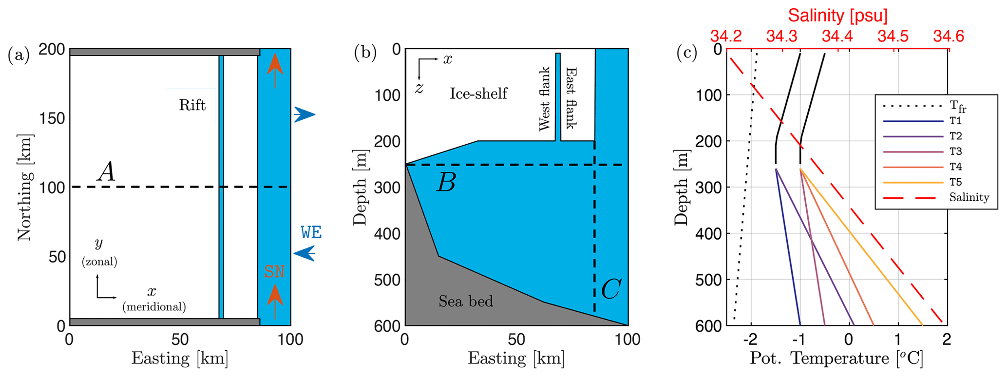
Figure 1Model domain sketches and ocean profiles. Panel (a) shows a schematic view of a horizontal cross section of the ice shelf (white), rift and ocean (blue), and seabed (grey) at 150 m depth. Red and blue arrows are directions of the alternating boundary conditions, which are termed here as south-to-north (SN) and westward-and-eastward (WE) flow. In the simulations with a rift, the west flank of the rift is fixed at 67.5 km to the east. Beside runs with an intact shelf, the rift is introduced with a width of 1, 2 and 3 km and is filled with 15 m of ice shelf. Panel (b) shows a schematic view of a vertical cross section of the model domain at 100 km to the north. Dashed black lines labeled A, B and C are horizontal and vertical cross sections useful to visualize model results. Panel (c) shows potential temperature and salinity profiles as initial and boundary conditions of the sensitivity experiments. Solid lines are initial and boundary conditions of temperature for “cold-water” and “warm-water” regimes. Cold and warm profiles are characterized by two (T1, T2) and three (T3, T4, T5) bottom temperatures. The dashed red line is the salinity profile and is constant in all experiments. The dotted black line is the freezing temperature of seawater (Tfr).
We employ an idealized ice shelf–ocean model configuration that relies on a Cartesian coordinate system (100 km × 200 km × 600 m, Fig. 1a–b) on a f plane with Coriolis frequency set to −1.4 × 10⁻⁴ rad s−1, which corresponds to a latitude of 75∘ S. Horizontal and vertical grid spacings are set to 250 and 10 m, which constrains the time step to 30 s in order to ensure numerical convergence. The model relies on an isotropic mesh and uses a partial cell formulation (Adcroft et al., 1997) with a minimum open cell fraction of 30 %. It is significant to acknowledge that the resolution employed here does not resolve melt-driven plumes (Xu et al., 2012; Burchard et al., 2022) nor the physics of frazil ice accretion within the water column.
The ice-shelf thickness at the ice front (located 85 km to the east) is set to 200 m slightly increasing to 250 m from 35 km to the east along the ice-shelf slope towards the grounding line (0 km to the east). Our simulations include a rift as a discontinuity in the ice-shelf draft. Its west flank is located at a fixed distance (67.5 km) from the grounding line, and rifts are introduced with variable width. Melting and freezing processes are active at horizontal and vertical interfaces between the ice and ocean, including the ice base, ice front, rift top and rift sidewalls. Since the ice-shelf geometry is fixed in time, the location of the ice–ocean interfaces does not change with melting and freezing.
Furthermore, the rift is filled with 15 m of ice shelf as a buffer layer between the atmosphere and ocean, which approximates an “ice-capped” rift and does not aim to reproduce ice mélange properties. Although ice mélange is often thought to be controlled by processes that are similar to those of sea ice, evidence shows that the heterogeneous material filling kilometer-wide rifts reaches thicknesses that are 1 to 2 orders of magnitude larger than sea ice (Orheim et al., 1990; Breyer and Fricker, 2022). Such a thick layer of ice can completely separate the liquid ocean from the atmosphere (Khazendar and Jenkins, 2003). By adopting the “ice-capped” approximation, we only focus our analysis on sub-shelf ocean processes introduced by the rift, while atmospheric and sea ice formation processes in the open ocean are neglected in this study.
The bathymetry consists of a prograde slope, deepening from the grounding line depth of 250 m to a maximum depth of 600 m at the eastern boundary (100 km to the east). A grounding line depth between 200 and 300 m, while relatively shallow, is characteristic of ice shelves such as some regions of the Larsen C ice shelf in the eastern Antarctic Peninsula (cold water) or the Wilkins and Bach ice shelves in the West Antarctic Ice Sheet (warm water). Furthermore, despite the fact that bathymetric sills and wedges can substantially alter the sub-shelf circulation by squeezing the water column and acting as a topographic barrier (Bradley et al., 2022), their presence is not considered here in order to generalize the seabed geometry as far as possible.
Finally, it is important to note that our simulations discard sub-glacial discharge at the grounding line. While this assumption may neglect important mixing processes where the ice shelf detaches from the underlying bedrock (Wei et al., 2020; Nakayama et al., 2021), it helps to focus our analysis on the impact of on-shelf water intrusion and its interaction with the rift.
2.2 Simulation design
We performed a total of 120 simulations with combinations of rift width, ocean temperature, velocity and direction of ocean currents flowing in the open ocean (Table 1).
Table 1Matrix of sensitivity experiments. Our study addresses the sensitivity of sub-shelf ocean dynamics, for a total of 120 experiments, to four rift width configurations, two flow directions, three flow velocities and five temperature profiles. In the following naming schema, R refers to rift width of 0 (intact shelf), 1, 2, or 3 km; SN/WE1-10 refers to velocity at the open boundaries for south-to-north and westward-and-eastward cases with an intensity of 1, 5, or 10 cm s−1; and T refers to temperature. Experiments highlighted in bold are chosen as representative cases and discussed in Sect. 3.2–3.4.
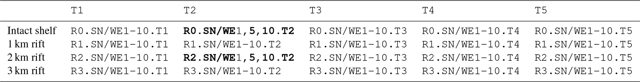
Our simulations include a rift as a discontinuity in the ice-shelf draft, which is introduced with a width of 1, 2 or 3 km, beside a control run with an intact ice shelf (no rift). Ocean circulation in the open ocean is prescribed as an inflow of varying magnitude (1, 5 and 10 cm s−1) as Dirichlet boundary condition at the open-ocean section of the south, north and east boundaries. We perform two sets of experiments with alternating open boundaries (Fig. 1a). In the first – which we term here as the south-to-north flow case (SN) – we “close” the eastern boundary (non-penetration condition) and prescribe an inflow at the southern boundary which is balanced by an outflow at the northern boundary to conserve mass. In the second – which we term here as westward-and-eastward flow case (WE) – we close northern and southern boundaries, and at the eastern bound we impose an inflow between 0–100 km to the north that is balanced by an outflow between 100–200 km to the north. The SN scenario can be seen as an idealization of along-ice front ocean currents, while WE cases represent across-shelf currents.
We initialize and force the simulations with idealized temperature–salinity profiles, distinguishing between “warm” and “cold” regimes, which are prescribed as initial and boundary conditions (Fig. 1c). Each profile is characterized by a mixed layer for the upper 250 m, which linearly changes to (a) two different bottom temperatures in the cold regime and (b) three different bottom temperatures in the warm regime (−0.5 ∘C in experiment T3, 0.5 ∘C in T4 and 1.5 ∘C in T5). The salinity profile increases linearly from 34.2 psu at the surface to 34.6 psu at 600 m depth in all experiments. The chosen temperature profiles are representative of temperature ranges observed near ice shelves in Antarctica (Orsi and Whitworth, 2004). Warm-water ice shelves in the Amundsen and Bellingshausen seas are represented by experiments under T5 forcing. In contrast, cold scenarios under T1 are similar to real conditions of cold-water ice shelves in the Weddell and Ross seas. The remaining scenarios (T2-T4) can be seen as representative of “in-between” ice shelves, e.g., Totten Ice Shelf on the Sabrina Coast.
2.3 Formal analysis
All experiments are integrated for 7 years. A quasi-steady state is reached in all simulations during the fifth year. To assess the impact of the rift in the sub-shelf dynamics, we focus on differences in modeled melt rate (equations in Appendix A1), heat transport toward the ice shelf interior (equations in Appendix A2) and sub-shelf circulation between simulations with intact and rifted ice shelves. To do so, we use average values from the last year of integration unless differently specified.
The discussion on the sub-shelf circulation and entrainment of water masses under the ice shelf is supported by the temporal evolution of virtual passive tracers. Tracers are initially released in the ice shelf cavity (tr01) and in the rift (tr02), with concentrations set at 1.0 at the beginning of the fifth year. Passive tracers do not affect the local density and advect with the local water flow for 2 years until the end of the simulations.
Section 3.1 presents and discusses spatially averaged melt rates and heat transport toward the interior of the ice shelf cavity across the 120 experiments, with emphasis on the sensitivity of basal melt to rift widths, thermal ocean forcing, and the magnitude and direction of off-shelf ocean currents.
Furthermore, we focus on the differences between intact and rifted simulations while sensitivity parameters are fixed to temperature profile T2 and current velocity of 5 cm s−1 in either the SN or WE direction, unless differently specified. This subset is chosen as representative simulations. Section 3.2 shows the distribution of melt rate along the ice-shelf base discussing differences between intact and rifted experiments. Moreover, Sect. 3.3 shows the distribution of melt and freeze rates along the rift surfaces. Finally, Sect. 3.4 discusses the sub-shelf circulation by analyzing the barotropic streamfunction and the evolution of passive tracers tr01 and tr02 under intact and rifted ice shelves. The temporal evolution of the horizontal distribution of tr01 across a horizontal cross section of the model domain (255 m, cross section B in Fig. 1b) is provided in the Supplement.
3.1 Average melt rate across all simulations
In order to summarize the impact of the selected sensitivity parameters on ice-shelf melting, we calculate spatially averaged melt rate integrated along (a) an ice-shelf base and (b) rift surfaces (both rift top and sidewalls are active ice–ocean interfaces) for the 120 simulations (Fig. 2). The intrusion of off-shelf water supplies the heat for melting the ice base, and our simulations show that heat transport toward the grounding line increases with higher thermal forcing (Fig. 3), with a consequent increase in basal melt rate for higher ocean temperatures.
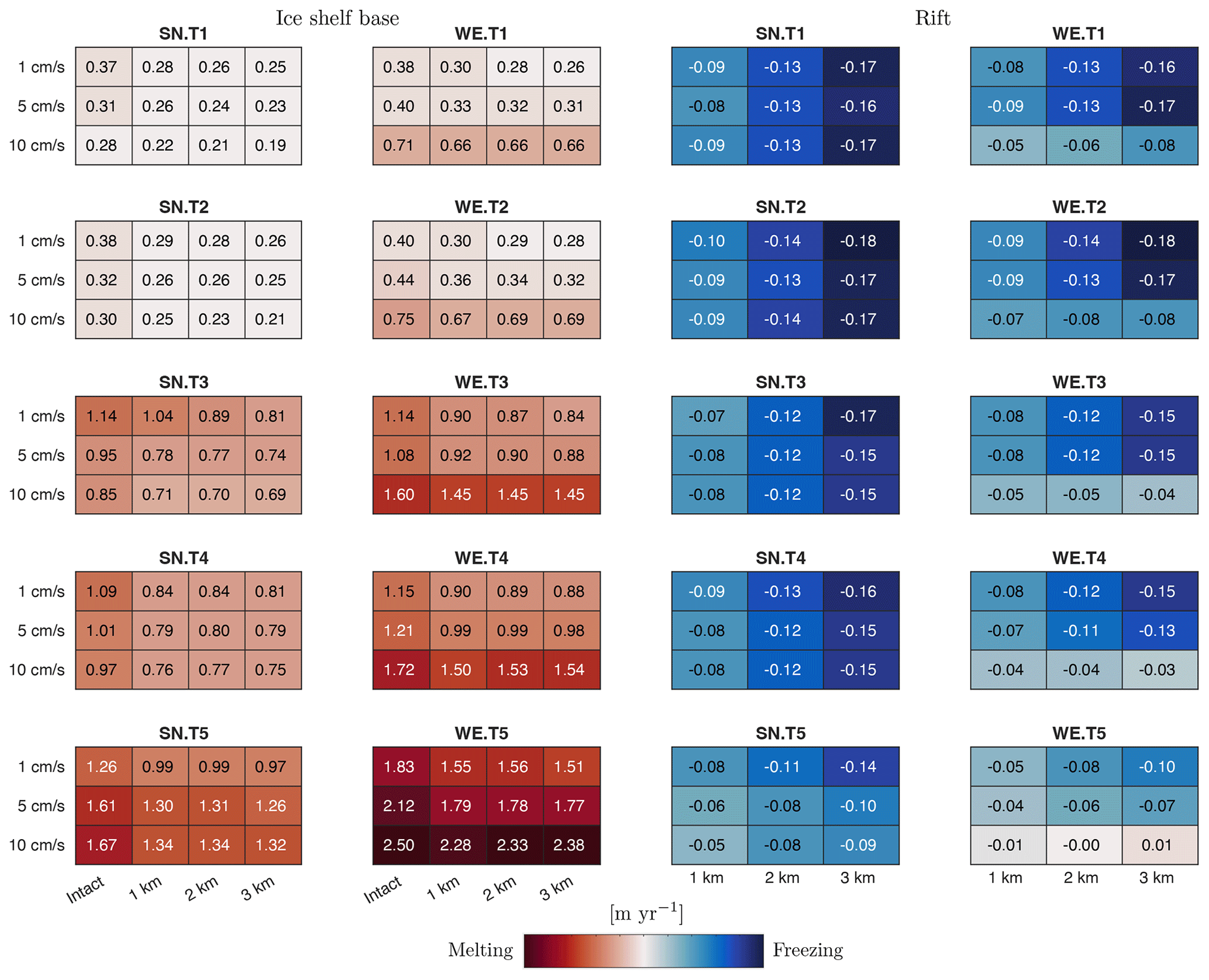
Figure 2Heat maps of average melt rate integrated along the ice-shelf base and in the rift for the 120 sensitivity experiments. Values are calculated with respect to temperature profile (panel), flow velocity (row) and rift width (column).
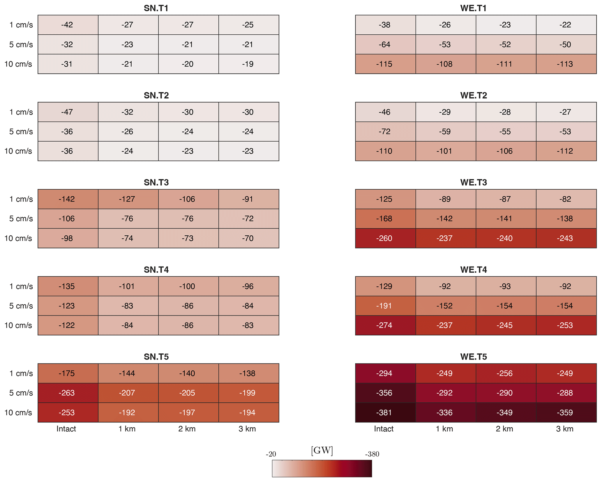
Figure 3Heat maps of total heat transport HT (Eq. A4) across the meridional cross section passing through the ice front (85 km to the east, cross section C in Fig. 1b) for the 120 sensitivity experiments. The negative sign means that the heat transport is directed toward the ice cavity interior. Values are calculated with respect to temperature profile (panel), flow velocity (row) and rift width (column).
Furthermore, the intensity of basal melt depends on the direction and velocity of the applied boundary condition. In order to conserve potential vorticity, ocean flow tends to maintain its motion along lines of constant depth (isobaths). Thus, water columns are “stiff” in the vertical direction (Taylor columns) and tend to deflect along isobaths. In our case, isobaths are parallel to the ice front by model design. The abrupt gradient in the water column thickness that is introduced by the ice front therefore acts as a barrier that limits the flow entering the cavity (e.g., Grosfeld et al., 1997; Wåhlin et al., 2020).
Our WE experiments are a representation of across-shelf water currents that are forced perpendicularly to the ice front and are therefore associated with stronger on-shelf mass and heat intrusion as the forced flow across isobaths intensifies. As a consequence, basal melt increases with stronger WE flow and large melt occurs near the ice front (further discussion in Sect. 3.2), regardless of thermal forcing and/or rift presence and width. On the other hand, SN simulations are representative of along-front water currents. Stronger SN currents therefore imply an enhanced tendency of the flow to follow along-front isobaths and, in turn, to further isolate the ice shelf cavity from mass and heat intrusion. As a consequence, SN experiments show a much lower heat intrusion when compared to WE experiments, which also results in large melt differences. Furthermore, we find that intact SN experiments under thermal scenarios T1 to T4 show a drop in melt rate with a strengthening of the boundary flow. The only set of SN experiments that shares with WE the same trend between melt and boundary flow intensity are experiments under T5 forcing.
The reason behind this discrepancy in basal melt with respect to boundary flow between SN experiments T1-T4 and T5 resides in the higher heat transport that the latter boundary flow implies (heat transport in T5 is twice as large as in T4, Fig. 3, while T4 temperature is only 1 ∘C colder than T5). Extreme warm cases under thermal forcing T5 result in a much higher heat transport across the ice front in response to a stronger flow, with a consequent higher average melt rate. In this case, the largest contribution to the average melt rate increase is indeed concentrated near the ice front.
On average, across all experiments melting in rifted simulations is 20 % lower and the heat intrusion is 20 % weaker than that computed for intact shelves under an identical forcing scenario. Our simulations also show that melt rate generally decreases with rift widening in all SN experiments and in WE experiments forced with a weak boundary flow (1 and 5 cm s−1). The only exceptions are WE experiments under a 10 cm s−1 boundary flow, where basal melt increases with rift widening. The differences in melting with respect to rift presence and width can be further investigated by evaluating heat fluxes in the rift.
The melt regime inside the rift is indeed very different from the ice-shelf base, as we find that this environment is dominated by freezing in almost all experiments. The only exceptions are WE experiments at 10 cm s−1 under thermal forcing T5, where freezing in a 3 km rift is stopped. Following the three-equation model (Appendix A1), melting at the ice base freshens the ambient water and increases its buoyancy, while freezing in the rift leads to water salinification and loss of buoyancy. These processes can also be quantified as a (negative) salt flux at the rift base (Fig. B1), whose intensity trends match the dependency of freezing rate with respect to sensitivity parameters. Freeze distribution along the rift surfaces is further investigated in Sect. 3.3.
Freeze rate in the rift shows the same dependency on thermal forcing as the basal melt rate discussed above. As the ocean temperature increases, freezing processes in the rift are inhibited and freeze rate decreases. However, differently than in the case of basal melt, we find that strengthening the boundary currents returns a negligible impact on the freeze rate in most experiments. The only exceptions are SN experiments under thermal forcing T5 and WE experiments at 5 and 10 cm s−1, where the stronger currents lead to progressively lower freeze rate.
Finally, we find that freezing in the rift and the associated salt flux at the rift base increases with rift widening in almost all experiments, with the only exception being WE experiments under a 10 cm s−1 boundary flow. The anomaly of this last case can be explained with the analysis of the melt and freeze pattern in the rift and its dependency to rift width (Sect. 3.3).
3.2 Melt pattern at the ice-shelf base
In this section, we discuss the basal melt distribution along the ice-shelf base and the calculated anomalies between intact and rifted shelves.
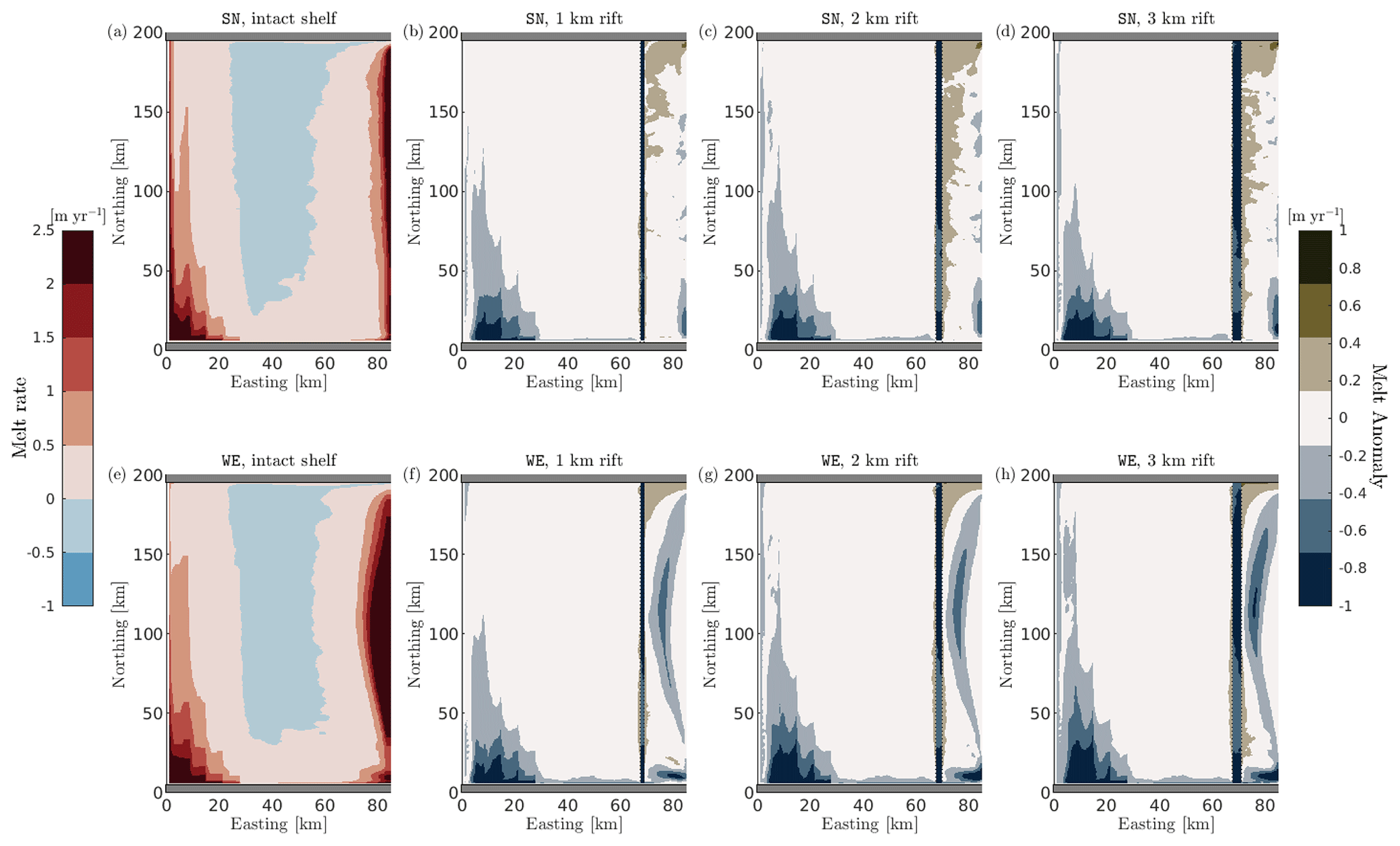
Figure 4Comparison of horizontal distribution of ice-shelf basal melt rates for different rift widths. Upper (a–d) and lower panels (e–h) correspond to SN and WE boundary currents of 5 cm s−1, respectively. The cold temperature profile T2 is used for all simulations. The first column shows the horizontal distribution of melt rate of intact experiments (a, e). Panels (b)–(d) and (f)–(h) show the horizontal distribution of melt anomaly, which is calculated as the difference between melt rate in the rifted shelf simulations with respect to intact cases under the same forcing conditions. The left color bar refers to melt rate, while the right color bar refers to melt anomaly.
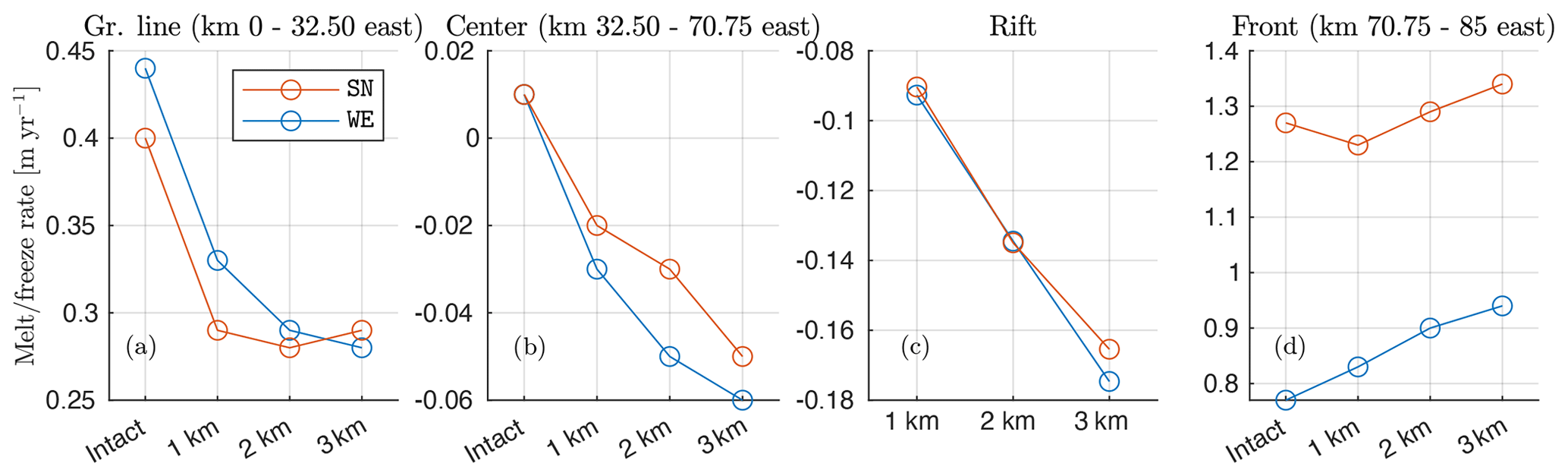
Figure 5Spatially averaged melt and freeze rate as a function of rift width for the three regions defined as grounding line, center and front. Values are referring to SN and WE experiments at 5 cm s−1, while the temperature profile is fixed to T2. Positive values mean melting, and negative values mean freezing.
For simulations with an intact shelf, it is possible to distinguish three meridional regions (Fig. 4a, e). These are characterized by distinct melting regimes, which can be quantified with the spatially averaged melt rate over the chosen regions (Fig. 5). We term these regions as grounding line (0–32.50 km to the east), center (32.50–70.75 km to the east) and front (70.75–85 km to the east). The westernmost region of intact experiments, adjacent to the grounding line, is dominated by similar average melt between SN and WE cases. These are also the deepest sections of the ice shelf (255 m), and we show in Sect. 3.3 that fresh meltwater that is formed here tends to buoyantly rise along the ice-shelf slope. The shallower center region (200 m) shows large patches of water freezing, as water drops below the freezing temperature, since this increases with lower pressure. On average, this region melts at a negligible rate in both SN and WE intact experiments. Finally, the front region – directly in contact with water transport in the open ocean – returns melting rates that are about twice as large in the WE case with respect to the SN case.
The introduction of the rift results in a redistribution of heat along the entire ice-shelf base, which can be quantified in each meridional region identified for intact cases (Figs. 4, 5 and C1 for relative change). Some of the impact is found in the central region, where the rift is actually located. In the intact case, this region is dominated by slow melting. Freezing processes that occur in the rift here drive a reduction in melt rate, which is progressively reduced by increasing the rift width. As a consequence, central regions of rifted cases show a generalized freezing.
We indeed find that average freezing in the rift increases with larger rifts, with the only exception of WE experiments under 10 cm s−1. The general behavior is due to a progressively larger area that is brought in contact with cold water dropping below the freezing point, which increases with wider rifts.
The presence of the rift also leads to faster melting in the frontal region, where the model simulates a relative increase in melt rate of 2 % in the SN case and of 12 % in the case of WE on average with respect to intact cases. Finally, our model results show that the region adjacent to the grounding line in rifted experiments returns a negative anomaly in the average melt rate with respect to intact simulations. When the rift is introduced, the grounding line region results in 30 % less melt rate than in the intact case under both SN and WE. WE simulations also show a net drop in melt rate in this region with rift widening, while in SN cases rift widening results in a negligible impact.
3.3 Melt pattern in the rift
It has been already discussed how the majority of experiments show that, on average, the rift environment is dominated by freezing (Fig. 2). In this section, we address how freezing patterns are distributed along the rift boundaries. The following analysis refers to SN and WE experiments with a 2 km wide rift and boundary flow at 5 and 10 cm s−1 under thermal forcing T2.
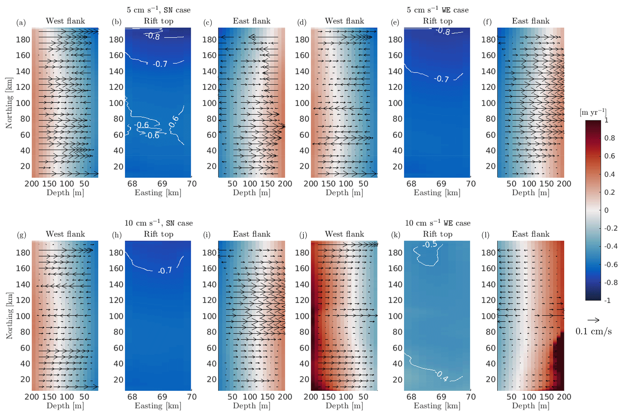
Figure 6Comparison of melt rate distribution (both color map and contour lines) along rift flanks and the top of a 2 km wide rift under 5 and 10 cm s−1 boundary forcing. The cold temperature profile T2 is used for all simulations. The west flank is closer to the grounding line, while the east flank is closer to the ice front (see Fig. 1b). Panels (a)–(f) correspond to SN and WE boundary currents of 5 cm s−1, while panels (g)–(n) correspond to boundary currents of 10 cm s−1. Positive values means melting, and negative values mean freezing. Arrows are vertical velocity along the rift flanks.
Along the rift sidewalls, our simulations show that melting occurs at their deeper levels and freezing at the top (Fig. 6). This bimodal pattern along the rift flanks is a result of the ice-pump mechanism active within the rift (Khazendar and Jenkins, 2003), as the freezing point of seawater increases with decreasing pressure. After melting in deeper sections of the rift, cold and fresh meltwater rises along the west flank (Fig. 6), following an overturning pattern that is similar to the “melt-driven” experiments of Jordan et al. (2014). Meltwater reaches the freezing point at a depth of around 120 m and water re-freezes above this level and at the rift top. Freezing in shallow portions of the rift leads to salinification of the ambient water and a consequent loss of buoyancy. The upwelling of buoyant water along the west flanks is generally balanced by the sinking of denser water along the east flank. We term the water mass that interacts with the rift as Rift Water. This water is tracked by passive tracer tr02, which is released in the rift environment at the beginning of the simulations. The downward transport of Rift Water can also be quantified as a (negative) salt flux through the rift base (Fig. B1).
While the SN flow increases from 5 to 10 cm s−1, the impact on the rift freeze is negligible (Fig. 6a–c to g–i). In contrast, strengthening the WE flow to 10 cm s−1 (Fig. 6d–f to j–l) has a major impact in the heat budget in the rift, as faster off-shelf water is forced to penetrate deeper in the westernmost regions of the ice cavity. This water can therefore intrude within the rift environment along the east flank (Fig. 6h), increasing melt rate of deeper level of the rift flanks and inhibiting freezing processes in shallower layers (Fig. 6j–l).
This behavior explains why WE experiments at 10 cm s−1 result in a progressive decrease in freezing rate with rift widening. Forcing the model with a 10 cm s−1 flow flushing the cavity perpendicularly to the ice front can reach the most inland section of the ice cavity when compared to weaker forcing and/or the SN set of experiments. As the east flank of the rift gets progressively closer to the ice front as the rift widens, off-cavity water eventually intrudes in progressively larger rifts (with a consequent switch in the sign of the salt flux across the rift base, Fig. B1) and inhibits freezing within. This behavior also explains that average basal melting increases with rift widening in the case of experiments WE under a strong 10 cm s−1 boundary flow until the extreme case of WE under thermal forcing T5 with a 3 km rift shows that the rift is dominated by slow melting (Fig. 2). On the other hand, the rest of the experiments (majority) show the opposite trend, where the larger the rift, the wider the area subjected to freezing (and hence the faster the average freezing rate). We should note that our assumption that the rift widens only toward the east (hence closer to the ice front) may bias these results. This is because the proximity of the rift to the open ocean could potentially obscure the actual effects of rift widening by promoting enhanced interaction with off-shelf water.
3.4 Sub-shelf circulation
In this section, we address how sub-shelf circulation and ocean stratification are affected by the rift presence using a modeled barotropic and overturning streamfunction together with the concentration of passive tracers tr01 and tr02 under the ice-shelf base.
3.4.1 Horizontal circulation
Our simulations show that the horizontal ocean dynamics under intact ice shelves is governed by the intrusion of off-shelf water, which is partially blocked by the ice front. The ice-shelf front indeed represents a sharp discontinuity in the water column thickness that acts as if the topographic barrier extended along the entire water column (Taylor–Proudman theorem). This limits the amount of off-shelf water that entrains the cavity, which tends to flow along isobaths (parallel to the ice front by model design) in order to conserve potential vorticity.
The simulated water transport in the open ocean (not shown here) is almost 6 times stronger in the WE experiments when compared to the SN case, despite their prescribed velocity at the boundary being the same. As the former boundary condition is applied to the east boundary, the flux of water entering in the model domain is much larger than the latter. As a further consequence, water transport flowing in the open ocean penetrates much further in the intact case forced with WE versus the case of SN (Fig. 7a, e). This also explains the larger melt rates in the proximity of the ice front for WE currents, where the ice is directly in contact with water transport in the open ocean (Fig. 4a, e).
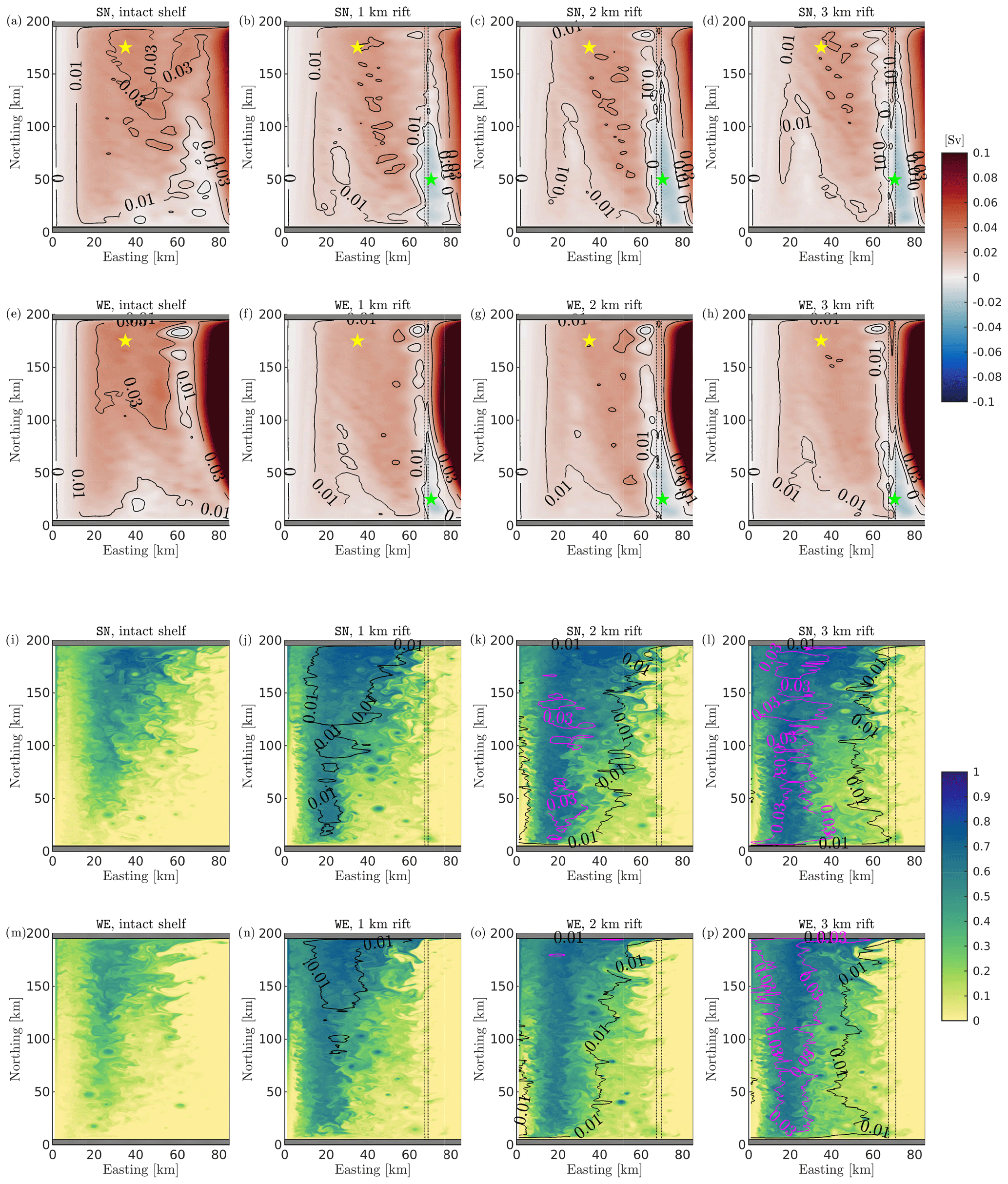
Figure 7Comparison of barotropic streamfunction and horizontal concentration of passive tracers for experiments with different rift widths. The first and third rows (second and fourth row) correspond to SN (WE) boundary currents of 5 cm s−1, respectively. The cold temperature profile T2 is used for all simulations. The dashed line is the rift location. Panels (a)–(h) compare the horizontal distribution of the barotropic streamfunction (both color map and contour lines). Positive values mean clockwise rotation, and negative values mean counterclockwise rotation. Locations marked with yellow and green stars are used to calculate intensity and the center of the two gyres. Panels (i)–(p) compare snapshots of the horizontal concentration of passive tracers tr01 (background color map) and tr02 (black and magenta contour lines corresponding to 0.01 and 0.03, respectively) at the grounding line level (255 m, cross section B in Fig. 1b) after 2 years from the initial release.
In both SN and WE experiments, inner regions of the ice shelf cavity are dominated by a cyclonic gyre, centered in the north section of the model domain (yellow star). This cyclonic system is driven by off-shelf water masses at −1.5 ∘C that entrain the cavity along the southern bound (Figs. 7i, m and D1a, e). This intrusion is also responsible for providing heat for melting the ice base (Fig. 3), while off-shelf water reaches and melts the westernmost extension of the ice shelf cavity. In turn, melting along the grounding line region drives the formation of buoyant meltwater (at around −1.9 ∘C), which flows northward along the ice shelf slope (Fig. D1i, m) and returns toward the ice front along the northern edge, closing the circulation pattern.
In the case of a rifted ice shelf, the intrusion along the southern bound resembles intact experiments. Nevertheless, the intensity of mass and heat intrusion toward the grounding line is to a large extent curtailed. The inhibition is caused by the rift, which represents a second discontinuity in the water column thickness. In order to follow the contours of constant depth and conserve potential vorticity, the intrusive water flow along the southern edge is deflected along the rift (Fig. 7b–d and f–h). This is shown by the fact that regions with low values of tr01 between 0 and 0.1 are confined seaward of the rift (Fig. 7j–l and n–p) while in the intact case low tr01 concentration is simulated through to 20 km to the east. On the other hand, tr02 – which tracks Rift Water formed after freezing processes in the rift – entrains the cavity from the rift base and spreads along the ice-shelf base, replacing off-shelf water. As a result, areas of the ice-shelf cavity eastward of the rift remain much cooler than in the intact case (Fig. D1a–h), and melt rate here is therefore reduced.
After the intrusion of off-shelf water is inhibited at the rift base, water transport westward of the rift is reduced as a consequence. The intensity of the cyclonic gyre progressively reduces by about 30 % in the case of a rifted shelf, with a negligible difference between SN and WE experiments. Differently from the intact case, water transport from the open ocean along the southern boundary is separated from the cavity interior by the formation of second gyre – anticyclonic and less intense – which is centered under the rift (green star, Fig. 7b–d and f–h).
Rift width determines the strength of the individual gyres and to a lesser degree their dimension. While the cyclonic gyre decreases in strength as ocean transport in westernmost region of the ice-shelf cavity is weaker, the model calculates a progressive growth in the anticyclonic gyre size with rift widening for both SN and WE sets of simulations, as the cavity remains colder (Fig. D1b–d and f–h) and melt rate reduces.
3.4.2 Overturning circulation
The calculated overturning streamfunction of intact experiments further shows that water transport under the ice base is to a large extent curtailed by the presence of the ice front (Fig. 9). However, a fraction of off-shelf water entrains the ice shelf cavity and the meridional on-shelf intrusion is strongest between 250 and 300 m (Fig. 8b, f). This intrusion drives the formation of a double overturning gyre system and delivers heat for melting the ice shelf in its deepest level, i.e., at the grounding line.
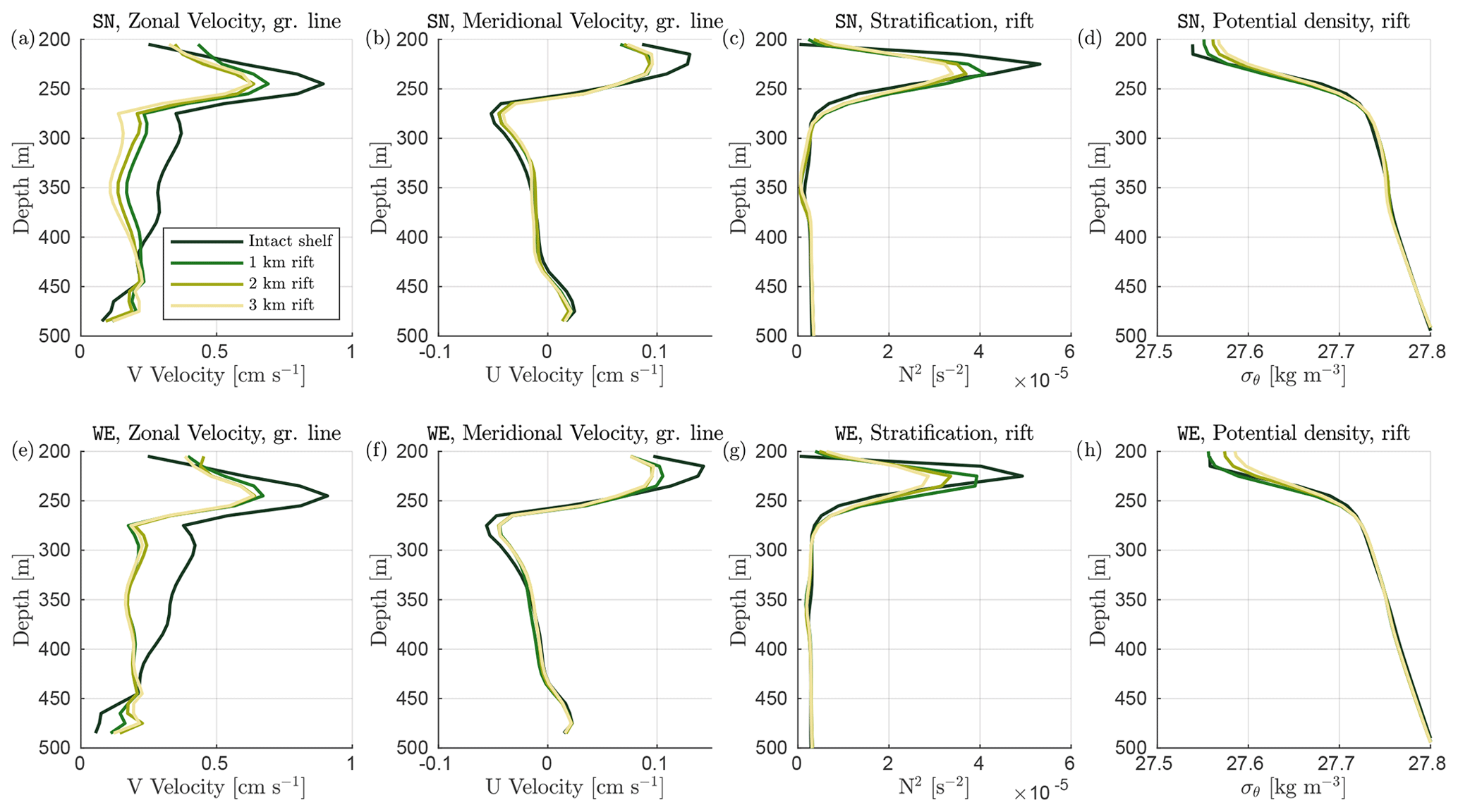
Figure 8Comparison of vertical ocean profiles for experiments with different rift widths. Upper (a–d) and lower panels (e–h) correspond to SN and WE boundary currents of 5 cm s−1, respectively. The cold temperature profile T2 is used for all simulations. Vertical profiles of meridional and zonal velocities – as the spatial average beneath the ice shelf slope (0–35 km to the east, 0–200 km to the north) – are in panels (a–b) and (e–f), respectively. Vertical profiles of buoyancy frequency squared (N2) and potential density anomaly ( kg m−3, where ρθ is the local potential density) – as the spatial average beneath the rift base (67.5–70.5 km to the east, 0–200 km to the north) – are in panels (c–d) and (g–h), respectively. Rift width is color coded.
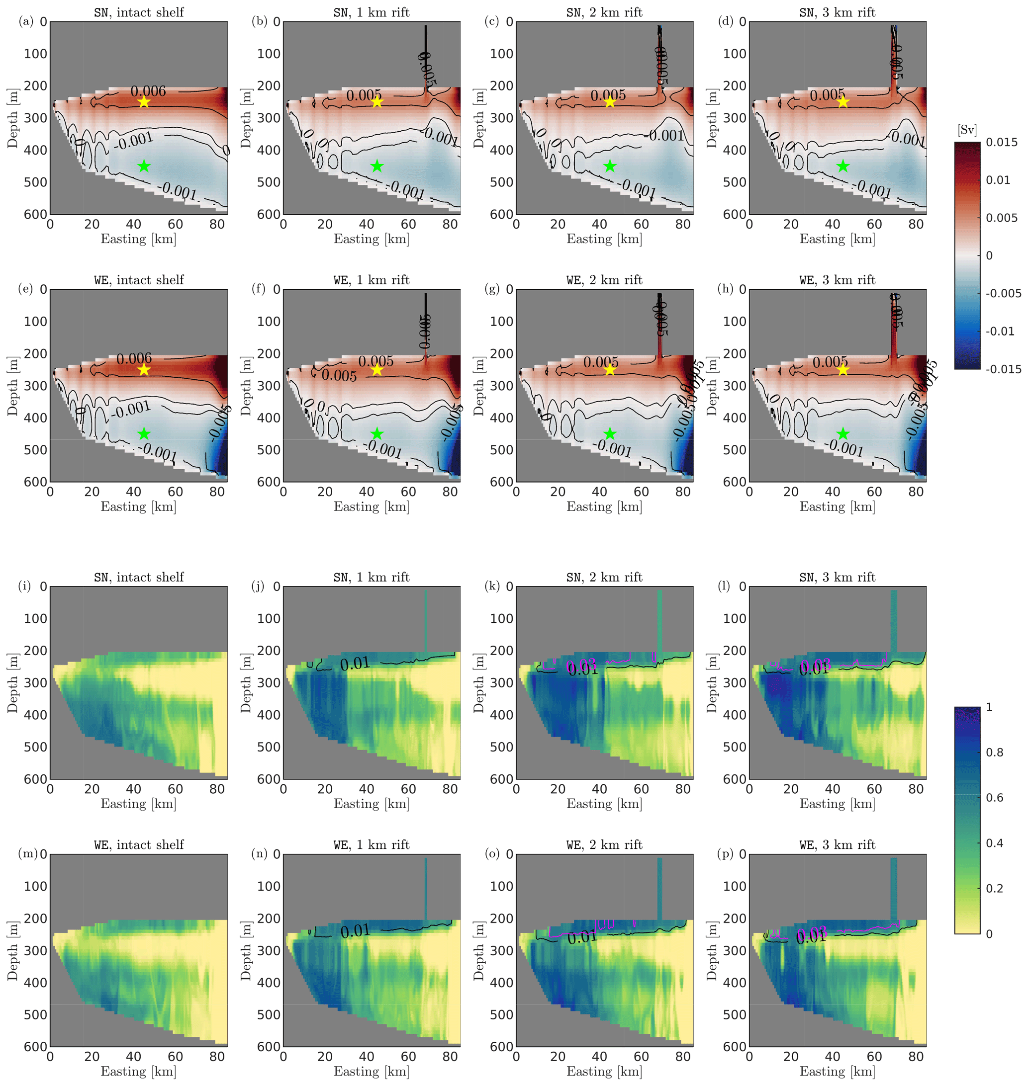
Figure 9Comparison of overturning streamfunction and vertical concentration of passive tracers for experiments with different rift widths. The first and third rows (second and fourth rows) correspond to SN (WE) boundary currents of 5 cm s−1, respectively. The cold temperature profile T2 is used for all simulations. Panels (a)–(h) compare the vertical distribution of the overturning streamfunction (both color map and contour lines). Positive values mean clockwise rotation, and negative values mean counterclockwise rotation. Locations marked with yellow and green stars are used to calculate intensity of the two overturning cells. Panels (i)–(p) compare snapshots of the vertical concentration of passive tracers tr01 (background color map) and tr02 (black and magenta contour lines corresponding to 0.01 and 0.03, respectively) at the zonal cross section along 50 km to the north (cross section A in Fig. 1a) after 2 years from the initial release.
Simulations with an intact shelf show a clockwise cell that is centered in the shallow portion of the ice cavity just beneath the ice base (yellow stars). Underneath the clockwise cell, our simulations show a further overturning transport of less intensity through a counterclockwise gyre cell (green stars), as water returns toward the ice front along the seabed (below 450 m, profiles in Fig. 8b, f). Furthermore, the vertical ocean profile of intact experiments resembles a stable stratified ocean interior where fresh and light meltwater overlays denser water. The pycnocline – the ocean layer where the density gradient is largest – is characterized by maximum stratification of s−2 calculated at a depth of 275 m (Fig. 8c–g).
In shallow layers of the model domain, water flows eastward along at the ice base, while melting at the grounding line is responsible for the increase in the buoyancy of the ambient water. The formed meltwater rises along the ice-shelf slope (Figs. 8b, f and D2) and is replaced by off-shelf water flowing toward the grounding line at depths, closing the shallow overturning circulation. Eventually, the upward flow of meltwater drops below the freezing point of seawater, driving water freezing in the central region of the model domain (Fig. 4).
In order to conserve potential vorticity, the intrusive water flow along the southern edge is deflected along the rift – which introduces an abrupt change in the isobath lines – and the off-shelf intrusion between 250 and 350 m is curtailed in response. As a consequence, our rifted simulations show that the clockwise gyre under the ice base in both SN and WE sets of experiments is 25 % weaker than in the intact case, while its continuity with transport in the open ocean is interrupted at the rift base.
Our model simulates that low values of tr01 are confined to seaward of the rift when this is present, while water layers immediately beneath the ice-shelf base are in contact with Rift Water (tr02). This water is formed after freezing in the ice rift and sinks due to decreased buoyancy. Sinking of Rift Water is also quantified by calculating the salt flux across the rift base (Fig. B1). The downwelling of Rift Water leads to spreading of saltier and denser water in the shallower layers of the ice-shelf cavity (Fig. 8d–h), weakening the sub-shelf stratification by up to 40 % (Fig. 8c–g).
The impact of rift widening is particularly evident in the distribution of the two tracers. While larger rifts contain more tr02, the concentration of Rift Water along the ice base increases. In contrast, the on-shelf penetration of water from the open ocean, which has low values of tr01, is gradually reduced in the westernmost areas of the ice cavity as the rift widens. While the density in the pycnocline increases, progressively stronger downwelling of Rift Water weakens the stratification under the ice-shelf base, cools the ambient water near the ice base and curtails basal melt.
Ice rifts and their impact on the circulation below and around ice shelves are generally neglected in ocean models, as employed resolutions are often too coarse to resolve kilometer-wide fractures in the ice shelf. In this study, we use the MITgcm at high resolution to show that the presence of a prominent rift near the ice-shelf front substantially alters the sub-shelf dynamics and the basal melt distribution. A schematic diagram of our findings is sketched in Fig. 10.
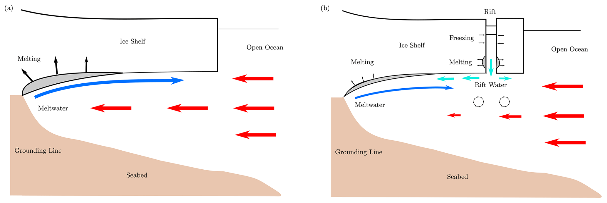
Figure 10Schematic diagram of ocean dynamics underneath an intact ice shelf (a) and a rifted ice shelf (b) in our idealized model. The introduction of the rift interrupts the on-shelf intrusion of off-cavity water from the open ocean toward the grounding line, responsible for supplying heat for melting the ice base. As a result, Rift Water floods the cavity from the rift base and basal melt is 20 % less than what is computed in the intact case, while the largest melt reduction occurs in proximity of the grounding line.
Our idealized ocean model simulates that, under intact ice shelves, transport of off-cavity water is inhibited by the presence of the ice front. This acts as a discontinuity in the water column thickness and limits the amount of flow entraining the ice cavity. Indeed, the water tends to flow along isobaths (in this case parallel to the ice front by model design) in order to conserve potential vorticity. A fraction of off-cavity water intrudes along the southern bound and provides the heat for melting the ice base. In turn, light meltwater formed after melting at the grounding line – i.e., the deepest layers of the idealized ice shelf – buoyantly rises along the ice draft toward the ice front, eventually dropping below the freezing point of seawater, as this decreases with depressurization. The sub-shelf circulation is closed as water returns toward the ice front along the northern edge (Fig. 7a, e).
We find that the introduction of an ice rift affects sub-shelf dynamics and distribution of basal melt by means of two processes. Firstly, the off-shelf water intrusion – which reaches and melts the grounding line – is further inhibited by the introduction of the rift. This acts as a second discontinuity in the water column thickness (Fig. 9) after the ice front and leads off-shelf water to deviate along the rift (Fig. 7). Secondly, in the case of a rifted ice shelf, off-shelf water intruding in the ice base is replaced by the outflow of dense Rift Water from inside the rift. This water is formed after seawater reaches the freezing temperature higher in the rift (Fig. 6) causing it to become more saline and sink. Modeled rift circulation is in good agreement with past numerical efforts (e.g., Khazendar and Jenkins, 2003), and the simulated overturning circulation resembles the “melt-driven” experiments of Jordan et al. (2014). Moreover, our simulations show that the downward flow of Rift Water weakens the stratification of the water column by supplying denser water close to the ice base (Fig. 8). As a consequence, the ambient water under rifted ice shelves is much cooler than in intact experiments (Fig. D1a–h) and the basal melt rate is curtailed in response (Fig. 4).
In perspective, the deflection of ocean currents along sharp discontinuities in the depth contour also occurs when the abrupt gradient is introduced at the bottom of the water column. For example, Menemenlis et al. (2007) showed that including a deep and narrow trench (the equivalent of a rift but extruded in the seabed) passing through the middle of Gibraltar Strait from the Atlantic Sea to the Mediterranean Sea substantially reduces the ocean current transport across the strait. In those experiments, ocean currents are deflected along the trench and in part dissipated by outflowing from inside the trench, similar to what happens in our simulations after the intrusive flow enters the ice shelf cavity and interacts with the rift.
Across the tested range of parameters, we quantify that – in rifted simulations – the heat transport toward the grounding line is 20 % weaker and the melt rate 20 % lower than in the case of an intact ice shelf under the same dynamic and thermodynamic forcing scenario (Figs. 2 and 3). In particular, we estimate that melt rate in proximity of the grounding line represents the largest anomaly with a decrease of 30 % when the rift is present. This result showcases the potential of rifts formed near the ice front to impact the dynamics of the most vulnerable areas of ice shelves.
Our simulations indeed suggest that the impact of rifts in the sub-shelf circulation may have implications in the dynamics of the grounding line, whose migration is extremely sensitive to off-shelf water incursion (e.g., Seroussi et al., 2017). An accurate estimation of melt patterns at the grounding line is important as sustained melt in these vulnerable locations leads to further ungrounding of continental ice, which in turn accelerates ice discharge from outlet glaciers into the ocean (Rignot and Jacobs, 2002). Thanks to our high-resolution model, we have shown how off-shelf water intrusion may be modulated by the presence of an ice rift near the ice front and by the formation of Rift Water from freezing processes within the rift. Rift Water may mix with water masses flowing toward the grounding line possibly re-distributing heat under the ice base. Finally, our simulations also show that the rift presence tends to modulate heat intrusion regardless of whether currents in the open ocean are directed across or along the ice front.
As a precise representation of the ice shelf cavity geometry is essential to correctly reproduce sub-shelf dynamics (Goldberg et al., 2012; Schodlok et al., 2012), we posit that high-resolution ocean models should account for the presence of ice rifts in order to accurately reproduce heat intrusion under the ice shelf and the – yet largely unexplored – impact of rifts in the sub-shelf ocean dynamics.
It is worth noting that our idealized model setup has a limitation in that it does not account for sub-glacial discharge, the impact of which is only starting to be investigated under Antarctic ice shelves (Wei et al., 2020; Nakayama et al., 2021). Simulations that include freshwater flux at the grounding line have demonstrated an increase in basal melt in these critical areas, leading to an improvement in the modeling of high melt rates observed under warm-water ice shelves in the West Antarctic Ice Sheet. Further numerical efforts are required in order to evaluate the impact of sub-glacial discharge under cold-water ice shelves and the interplay with the processes presented here.
Although our simulations introduce novel sub-shelf processes that have been neglected in past ice–ocean modeling efforts, our idealized model setup cannot accurately quantify the effective importance of rifts in the sub-shelf dynamics of actual ice shelves. In particular, sea ice processes near the ice front are key components in mixing processes under and near the ice shelf. For example, dense High Salinity Shelf Water is formed by brine rejection during winter sea ice formation. Besides being an important contributor to the Meridional Overturning Circulation and the Antarctic Bottom Water (e.g., van Caspel et al., 2015), High Salinity Shelf Water convects down near the coast due to its buoyancy. These cold and dense water masses flow in deeper sections of the ice cavity and perturb the water ambient at depth (e.g., Nicholls et al., 2009). These mixing processes are controlled by atmospheric forcing, with implications that go beyond the scope of our study. The inclusion of sea ice processes and their impact on water masses near the front of a rifted ice shelf in future numerical efforts is therefore necessary to accurately understand ocean dynamics and heat intrusion in the ice shelf cavity. This is particularly relevant where winter sea ice production is abundant (e.g., large ice shelves in the Weddell Sea). To this end, our work suggests that the downwelling of dense Rift Water may imply a further layer of complexity in the mixing processes near the ice front and is therefore worthy further investigation.
Furthermore, observations have shown frazil ice crystals that are suspended in buoyant plumes within the rift and adherent to the rift sidewalls and top in form of marine ice (Orheim et al., 1990; Lawrence et al., 2023). Meltwater that is adherent to the ice base and the rift flanks can reach the supercooled state due to decompression, forming frazil ice crystals suspended in the water column. Jordan et al. (2014) estimates that the total freezing occurring inside a rift is mainly due to frazil ice accretion processes. Nevertheless, computational constraints and the vertical resolution employed here do not allow us to resolve (a) non-hydrostatic processes such as melt-driven plumes (Xu et al., 2012; Burchard et al., 2022) or (b) frazil ice crystals suspended within these plumes. These are caveats to our study as the entrainment into the plume determines the heat transferred to the ice and hence the melt rate (Vreugdenhil and Taylor, 2019). Similarly, frazil ice accretion impacts the stratification under the ice shelf and the buoyancy of such melt-driven plumes (Jenkins and Bombosh, 1995). For instance, suspended frazil ice crystals may enhance the buoyancy of the plume, leading to its acceleration and faster growth (Hewitt, 2020), but larger crystals precipitate more rapidly, reducing the buoyancy of melt-driven plumes. Future numerical efforts are required to constrain the role of non-hydrostatic processes within the rift and the impact of frazil ice formed in the rift in the stratification under the ice-shelf base.
Lastly, rift growth is episodic, with events that last from minutes to hours, often followed by periods of inactivity that can range up to several months and years (Bassis et al., 2005; Walker et al., 2015; Banwell et al., 2017). Rifts are often filled with ice mélange, whose rheological and mechanical properties are challenging to model (Vankova and Holland, 2017; Amundson et al., 2020). Although our simulations offer a highly simplified version of an ice rift – where atmospheric forcing and growth processes of encased ice mélange are neglected and rift width is fixed – they suggest that changes in rift size will cause a direct modulation of the amount of freezing between flanks (e.g., Figs. 2 and 4). Hence, mechanically induced rift propagation – altering rift size, e.g., due to ice heterogeneity (Borstad et al., 2017) – may directly influence thinning or thickening of encased ice mélange and thus the cohesiveness of rift flanks, in addition to being triggered by the variation in rift infill due to environmental warming (Holland et al., 2009; Larour et al., 2021).
Our study shows that resolving kilometer-wide rifts in the geometrical description of the ice-shelf cavity may imply a further layer of complexity in mixing processes below the ice base, with possible alteration of mass and heat intrusion. We estimate that these processes – so far largely unexplored – may alter ocean heat intrusion and melt rate by as much as 20 %. Notably, we calculate a significant 30 % increase in melt at the grounding line in simulations with a rift. Given the crucial importance of basal ablation on the ice-shelf stability – in particular where the ice shelf becomes afloat – the processes presented here are worthy of further investigation. On a larger scale, a better understanding of heat pathways toward the grounding line remains a fundamental research avenue that would improve the estimation of ice-shelf ablation and consequently the evolution of the Antarctic Ice Sheet in a warming climate.
A1 Three-equation model
Ice–ocean processes are governed by the three-equation model (Hellmer and Olbers, 1989; Jenkins, 1991; Holland and Jenkins, 1999). Melting and freezing form an ice–ocean boundary layer that is implemented in MITgcm as a heat flux and a “virtual” salt flux (i.e., a freshwater flux q without volume change in the ocean) at the water cell immediately adjacent to the ice interface. In MITgcm, the ice–ocean interface can be horizontal (Losch, 2008) or vertical (Xu et al., 2012). Melting (q<0) freshens the ambient water, while freezing (q>0) leads to seawater salinification. The three-equation model can be written as the heat (Eq. A1) and salinity budget (Eq. A2) for the boundary layer, together with the linear dependency of the freezing point of seawater Tfr with pressure (Eq. A3), in symbols as follows:
where cp = 4000 J kg−1 K−1 and cp,I = 2000 J kg−1 K−1 are the specific heat capacity of seawater and ice, respectively; L = 334 000 J kg−1 is the latent heat of fusion; κ = 1.54 × 10⁻⁶ m2 s−1 is the heat diffusivity through the ice; Δh is the ice shelf draft; ρ is the density of seawater; Tb and Sb are temperature and salinity at the boundary layer (water cell adjacent to the ice interface), respectively; T and S are local temperature and salinity, respectively; TI = −20 ∘C is the core temperature of the ice shelf; and p is the local pressure.
The freshwater flux q can be translated into melt rate using the density of ice ρI through . As we arbitrarily set that means melting and means freezing, larger absolute values of imply stronger melt or freeze rate depending on the sign. In this study, heat transfer coefficient γT is held constant to 10−4, and the salinity transfer coefficient γS is a function of γT after the ISOMIP experiments of Losch (2008). By assuming that the temperature at the boundary layer Tb is equal to the freezing point of seawater (Tfr), Eqs. (A1)–(A3) are numerically solved in MITgcm to obtain the triplet Tb, Sb, q, which represents the boundary condition applied at the ice–ocean interface.
A2 Heat transport toward the ice cavity interior
The heat transport HT across a meridional cross section x=x1 can be written as follows:
where is the local potential density, is the local meridional velocity, is the local potential temperature and Tfr is in situ freezing point of seawater. Heat maps of HT integrated across the ice front cross section x=85 km to the east for the 120 experiments are shown in Fig. 3. Sensitivity of HT with respect to rift width, boundary current and thermal forcing matches the pattern shown in heat maps of melt rate in Fig. 2 and is discussed in Sect. 3.1.
The salt flux ΦS across the rift base at depth m can be written as follows:
where Ar is the rift base area, is the vertical velocity and is the in situ salinity. Heat maps of ΦS integrated across the rift base for the 120 experiments are shown in Fig. B1.
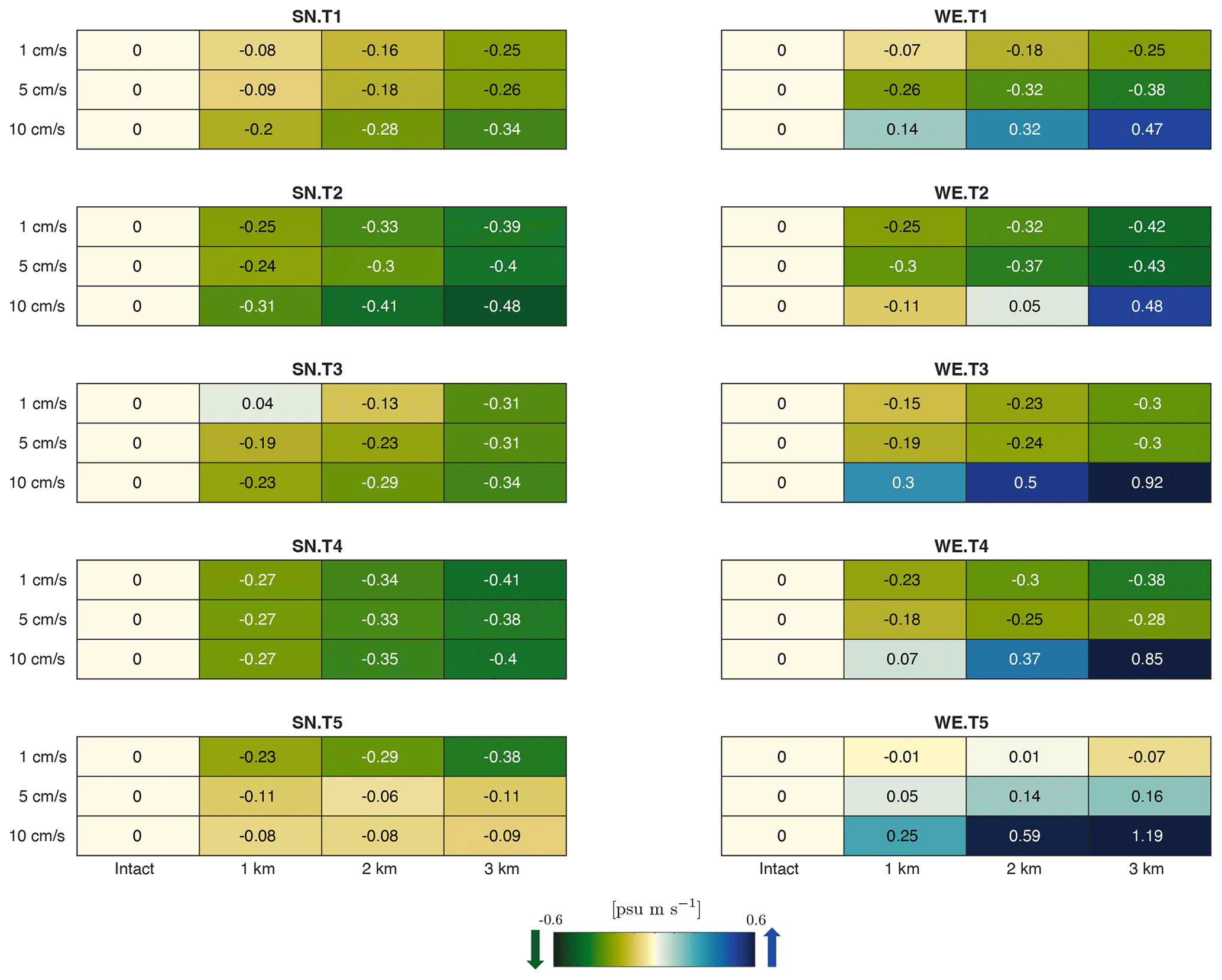
Figure B1Heat maps of total salt flux ΦS across the rift base (200 m) for the 120 sensitivity experiments. Positive and negative values mean upward and downward transport, respectively. Values are calculated with respect to temperature profile (panel), flow velocity (row) and rift width (column).
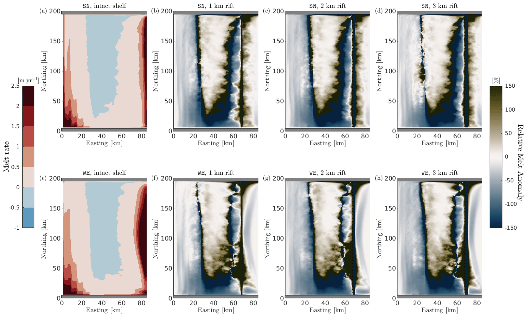
Figure C1Comparison of horizontal distribution of ice-shelf basal melt rates for different rift widths. The upper (a–d) and lower panels (e–h) correspond to SN and WE boundary currents of 5 cm s−1, respectively. The cold temperature profile T2 is used for all simulations. The first column shows the horizontal distribution of melt rate of intact experiments (a, e). Panels (b)–(d) and (f)–(h) show the horizontal distribution of relative melt anomaly, which is calculated as the difference between melt rate in the rifted shelf simulations with respect to intact cases under the same forcing conditions, which is then referenced to the results in the intact case. The left color bar refers to melt rate, while the right color bar refers to relative melt anomaly. It is important to note that there are some areas of the ice shelf that experience a switch from melting to freezing, which in terms of relative value is quantified as more than 100 % alteration, even if the absolute change is fairly small.
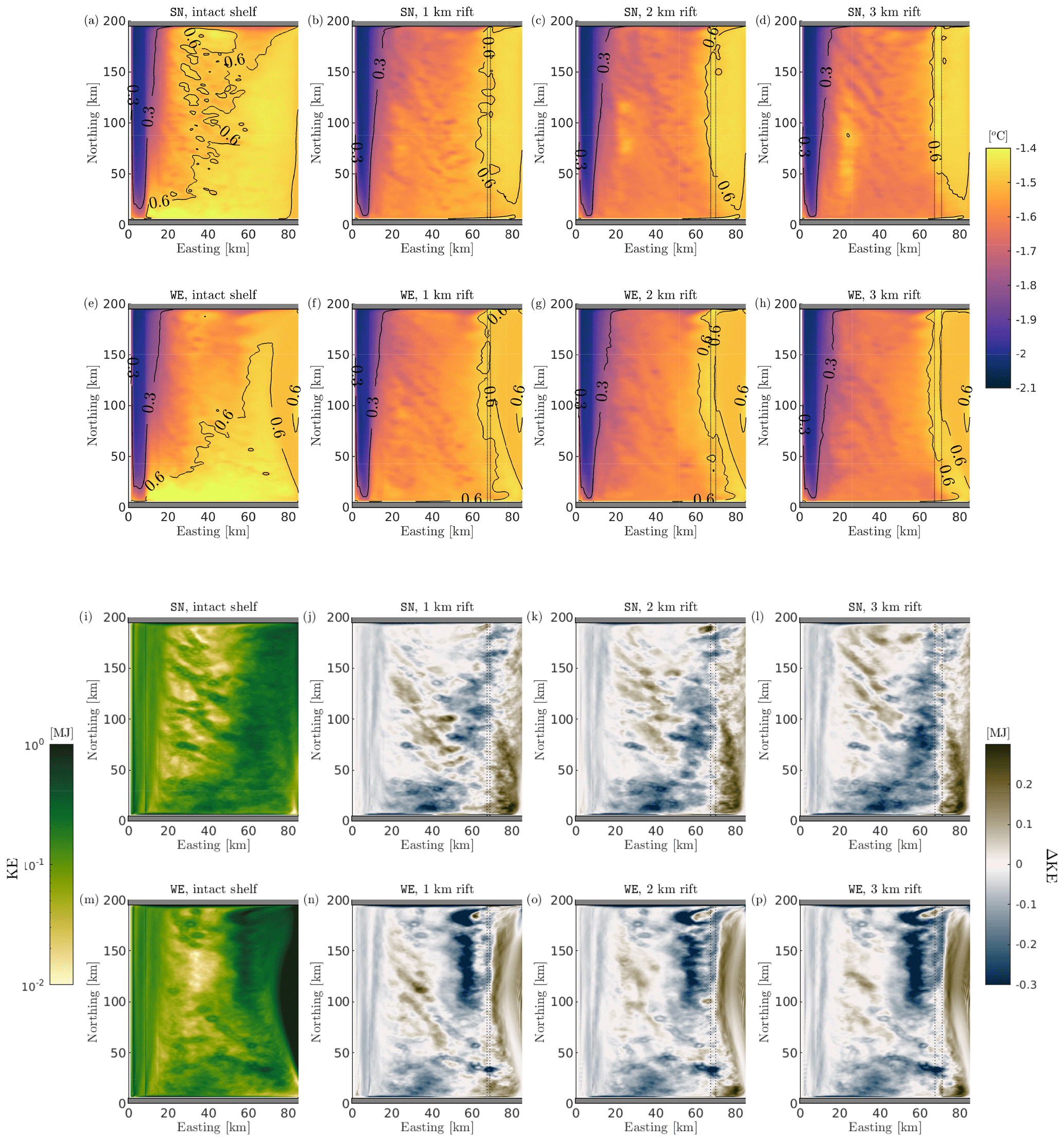
Figure D1Comparison of horizontal distribution of potential temperature and kinetic energy (KE) for different rift widths at the grounding line level (255 m, cross section B in Fig. 1b). The first and third rows (second and fourth rows) correspond to SN (WE) boundary currents of 5 cm s−1. The cold temperature profile T2 is used for all simulations. The dashed line is the rift location. Panels (a)–(h) compare the horizontal distribution of potential temperature (color map) and the difference between in situ potential temperature and the freezing point of seawater (black contour lines). Panels (i)–(p) compare the kinetic energy. The first column shows the horizontal distribution of kinetic of intact experiments (i, m). Panels (j)–(l) and (n)–(p) show the horizontal distribution of kinetic energy anomaly, which is calculated as the difference between kinetic energy at 255 m in the rifted shelf simulations with respect to intact cases under the same forcing conditions. The left color bar refers to kinetic energy, while the right color bar refers to kinetic energy anomaly.
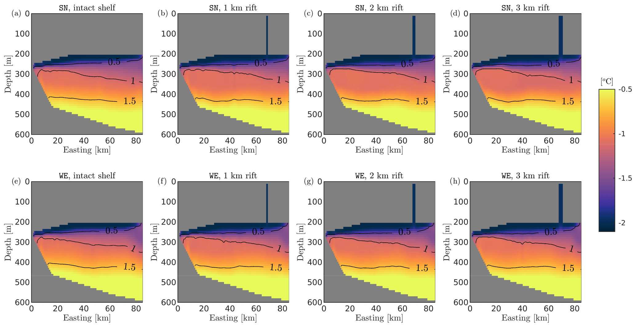
Figure D2Comparison of vertical distribution of potential temperature (color map) and the difference between in situ potential temperature and the freezing point of seawater (black contour lines) for experiments with different rift widths at the zonal cross section along 50 km to the north. Note that the values in the color bar are different to those of Fig. D1a–h. The first and third rows correspond to SN and WE boundary currents of 5 cm s−1, respectively. The cold temperature profile T2 is used for all simulations.
Ocean stratification can be calculated with the square of the Brunt–Väisäilä (buoyancy) frequency, which can be computed as the vertical buoyancy gradient:
where ρθ is the local potential density and g is the gravitational acceleration. N2 is a measure of the stability of a water column to convection and overturning. Positive values of N2 indicate a stable stratified fluid where lighter water overlays denser water. A negative value of N2 indicates an unstable water column where denser water is found above lighter water and convection and overturning processes increase.
MITgcm is an open-source numerical model, freely available on GitHub (https://github.com/MITgcm/MITgcm, last access: 2 June 2023; https://doi.org/10.5281/zenodo.3967889, Campin et al., 2020). All datasets and model outputs comprise 27 TB of data and are stored on the Lou mass storage system at the NASA Advanced Super-computing facility at Ames Research Center. Code and input data used to produce model output are freely available on GitHub (https://github.com/MPoinelli/Poinelli2023a_TC, last access: 2 June 2023) and Zenodo (https://doi.org/10.5281/zenodo.7905547, Poinelli, 2023).
The supporting animation shows the 2-year evolution of passive tracer tr01 distribution at the grounding line depth, 255 m, in cross section B in Fig. 1b. The supplement related to this article is available online at: https://doi.org/10.5194/tc-17-2261-2023-supplement.
MP conceived of and designed the model simulations, ran the experiments, analyzed the results, and wrote the manuscript. MS supported design and model setup. EL, MV, RR and MS discussed results and revised the manuscript.
The contact author has declared that none of the authors has any competing interests.
Publisher's note: Copernicus Publications remains neutral with regard to jurisdictional claims in published maps and institutional affiliations.
Part of the research was carried out at the Jet Propulsion Laboratory, California Institute of Technology, under a contract with the National Aeronautics and Space Administration (NASA). We gratefully acknowledge support from the NASA Cryospheric Sciences Program. High-end computing resources were provided by the NASA Advanced Supercomputing Division of the Ames Research Center. Color maps used in this paper are from Thyng et al. (2016). Mattia Poinelli sincerely thanks Yoshihiro Nakayama, Dimitris Menemenlis, Eric Rignot, Stefanie Nanninga and Ratnakar Gadi for stimulating discussions during the final stage of this research project. We express our gratitude to the Editor Nicolas Jourdain and the two anonymous referees for their thorough and insightful review, which greatly enhanced the clarity and impact of this manuscript.
Part of the research was carried out at the Jet Propulsion Laboratory, California Institute of Technology, under a contract with the National Aeronautics and Space Administration (NASA).
This paper was edited by Nicolas Jourdain and reviewed by two anonymous referees.
Adcroft, A., Hill, C., and Marshall, J.: The representation of topography by shaved cells in a height coordinate model, Mon. Weather Rev., 125, 2293–2315, https://doi.org/10.1175/1520-0493(1997)125<2293:ROTBSC>2.0.CO;2, 1997. a
Amundson, J., Kienholz, C., Hager, A. O., Jackson, R. H., Motyka, R. J., Nash, J. D., and Sutherland, D. A.: Formation, flow and break-up of ephemeral ice mélange at LeConte Glacier and Bay, Alaska, J. Glaciol., 66, 577–590, https://doi.org/10.1017/jog.2020.29, 2020. a
Banwell, A. F., Willis, I. C., MacDonald, G. J., Goodsell, B., Mayer, D. P., Powell, A., and MacAyeal, D. R.: Calving and rifting on the McMurdo Ice Shelf, Antarctica, Ann. Glaciol., 58, 78–87, https://doi.org/10.1017/aog.2017.12, 2017. a, b
Bassis, J. N., Coleman, R., Fricker, H. A., and Minster, J. B.: Episodic propagation of a rift on the Amery Ice Shelf, East Antarctica, Geophys. Res. Lett., 32, 1–5, https://doi.org/10.1029/2004GL022048, 2005. a, b
Borstad, C., McGrath, D., and Pope, A.: Fracture propagation and stability of ice shelves governed by ice shelf heterogeneity., Geophys. Res. Lett., 44, 4186–4194, https://doi.org/10.1002/2017GL072648, 2017. a
Bradley, A. T., Bett, D. T., Dutrieux, P., De Rydt, J., and Holland, P. R.: The Influence of Pine Island Ice Shelf Calving on Basal Melting, J. Geophys. Res.-Oceans, 127, e2022JC018621, https://doi.org/10.1029/2022JC018621, 2022. a
Breyer, C. and Fricker, H.: Spatiotemporal Analysis of ICESat-2 observation of Ice Mélange Thickness in Antarctic rifts, 2022 AGU Fall Meeting, 12–16 December 2022, Chicago, IL, USA, American Geophysical Union (AGU), 2022AGUFM.C32C0852B, 2022. a, b
Burchard, H., Bolding, K., Jenkins, A., Losch, M., Reinert, M., and Umlauf, L.: The vertical structure and entrainment of subglacial melt water plumes, J. Adv. Model. Earth Syst., 14, e2021MS002925, https://doi.org/10.1029/2021MS002925, 2022. a, b
Campin, J. M., Heimbach, P., Losch, M., Forget, G., Hill, E., Adcroft, A., Menemenlis, D., Chris, H., Jahn, O., Scott, J., Mazloff, M., Fox-Kemper, B., Nguyen, A., Doddridge, E., Fenty, I., Bates, M., Eichmann, A., Smith, T., Martin, T., Lauderdale, J., Abernathey, R., Deremble, B., Goldberg, D., Bourgault, P., and Dussin, P.: MITgcm/MITgcm: mid 2020 version (Version checkpoint67s), Zenodo [code], https://doi.org/10.5281/zenodo.3967889, 2020. a
Dinniman, M. S., Asay-Davis, X. S., Galton-Fenzi, B. K., Holland, P. R., Jenkins, A., and Timmermann, R.: Modeling Ice Shelf/Ocean Interaction in Antarctica: A Review, Oceanography, 29, 144–153, https://doi.org/10.5670/oceanog.2016.106, 2016. a
Doake, C. S. M., Corr, H., Rott, H., Skvarca, P., and Young, N.: Breakup and conditions for stability of the northern Larsen Ice Shelf, Antarctica, Nature, 398, 778–780, https://doi.org/10.1038/35832, 1998. a
Dupont, T. K. and Alley, R. B.: Assessment of the importance of ice-shelf buttressing to ice-sheet flow, Geophys. Res. Lett., 32, L04503, https://doi.org/10.1029/2004GL022024, 2005. a
Fuerst, J. J., Durand, G., Gillet-Chaulet, F., Tavard, L., Rankl, M., Braun, M., and Gagliardini, O.: The safety band of Antarctic ice shelves, Nat. Clim. Change, 6, 479–482, https://doi.org/10.1038/nclimate2912, 2016. a
Goldberg, D. N., Little, C. M., Sergienko, O. V., Gnanadesikan, A., Hallberg, R., and Oppenheimer, M.: Investigation of land ice-ocean interaction with a fully coupled ice-ocean model: 1. Model description and behavior, J. Geophys. Res., 117, 1–16, https://doi.org/10.1029/2011JF002247, 2012. a, b
Grosfeld, K., Gerdes, R., and Determan, J.: Thermohaline circulation and interaction between ice shelf cavities and the adjacent open ocean, J. Geophys. Res., 102, 15595–15610, https://doi.org/10.1029/97JC00891, 1997. a
Hellmer, H. H. and Olbers, D. J.: A two-dimensional model of the thermohaline circulation under an ice shelf, Antarct. Sci., 1, 325–336, https://doi.org/10.1017/S0954102089000490, 1989. a
Hewitt, I. J.: Subglacial Plumes, Annu. Rev. Fluid Mech., 52, 145–169, 2020. a
Holland, D. M. and Jenkins, A.: Modeling thermodynamic ice-ocean interactions at the base of an ice shelf, J. Phys. Oceanogr., 29, 1787–1800, 1999. a
Holland, P. R., Corr, H. F. J., Vaughan, D. G., and Jenkins, A.: Marine ice in Larsen Ice Shelf, Geophys. Res. Lett., 36, L11604, https://doi.org/10.1029/2009GL038162, 2009. a
IPCC: Summary for Policymakers, in: IPCC Special Report on the Ocean and Cryosphere in a Changing Climate, edited by: Pörtner, H.-O., Roberts, D. C., Masson-Delmotte, V., Zhai, P., Tignor, M., Poloczanska, E., Mintenbeck, K., Alegría, A., Nicolai, M., Okem, A., Petzold, J., Rama, B., and Weyer, N. M., Cambridge University Press, Cambridge, UK and New York, NY, USA, ISBN 1009157973, 2019. a
Jackett, D. R. and McDougall, T. J.: Minimal adjustment of hydrographic profiles to achieve static stability, J. Atmos. Ocean. Tech., 12, 381–389, https://doi.org/10.1175/1520-0426(1995)012<0381:MAOHPT>2.0.CO;2, 1995. a
Jenkins, A.: A one-dimensional model of ice shelf-ocean interaction, J. Geophys. Res., 96, 20671–20677, https://doi.org/10.1029/91JC01842, 1991. a
Jenkins, A. and Bombosh, A.: Modeling the effects of frazil ice crystals on the dynamics and thermodynamics of ice shelf water plumes., J. Geophys. Res.-Oceans, 100, 6967–6981, 1995. a
Jordan, J. J., Holland, P. R., Jenkins, A., Piggot, M. D., and Kimura, S.: Modeling ice-ocean interaction in ice-shelf crevasses, J. Geophys. Res.-Oceans, 119, 995–1008, https://doi.org/10.1002/2013JC009208, 2014. a, b, c, d
Khazendar, A. and Jenkins, A.: A model of marine ice formation within Antarctic ice shelf rifts, J. Geophys. Res., 108, 3235, https://doi.org/10.1029/2002JC001673, 2003. a, b, c, d
Large, W., McWilliams, J., and Doney, S.: Oceanic vertical mixing: A review and a model with nonlocal boundary layer parameterization, Rev. Geophys., 32, 363–403, https://doi.org/10.1029/94RG01872, 1994. a
Larour, E., Rignot, E., Poinelli, M., and Scheuchl, B.: Processes controlling the rifting of Larsen C Ice Shelf, Antarctica, prior to the calving of iceberg A68, P. Natl. Acad. Sci. USA, 118, 1–8, https://doi.org/10.1073/pnas.2105080118, 2021. a, b
Lawrence, J. D., Washam, P. M., Stevens, C., Hulbe, C., Horgan, H. J., Dunbar, G., Calkin, T., Stewart, C., Robinson, N., Mullen, A. D., Meister, M. R., Hurwitz, B. C., Quartini, E., Dichek, D. J. G., A., S., and Schmidt, B. E.: Crevasse refreezing and signatures of retreat observed at Kamb Ice Stream grounding zone, Nat. Geosci., 16, 238–243, https://doi.org/10.1038/s41561-023-01129-y, 2023. a, b
Lewis, E. L. and Perkin, R. G.: Supercooling and Energy Exchange Near the Arctic Ocean Surface, Geophys. Res. Lett., 88, 7681–7685, https://doi.org/10.1029/JC088iC12p07681, 1983. a
Lipovsky, B. P.: Ice shelf rift propagation: stability, three-dimensional effects, and the role of marginal weakening, The Cryosphere, 14, 1673–1683, https://doi.org/10.5194/tc-14-1673-2020, 2020. a
Losch, M.: Modeling ice shelf cavities in a z coordinate ocean general circulation model, J. Geophys. Res.-Oceans, 113, C08043, https://doi.org/10.1029/2007JC004368, 2008. a, b
Menemenlis, D., Fukumori, I., and Lee, T.: Atlantic to Mediterranean Sea Level Difference Driven by Winds near Gibraltar Strait, J. Phys. Oceanogr., 37, 359–376, https://doi.org/10.1175/JPO3015.1, 2007. a
Morlighem, M., Rignot, E., Binder, T., Blankenship, D., Drews, R., Eagles, G., Eisen, O., Ferraccioli, F., Forsberg, R., Fretwell, P., Goel, V., Greenbaum, J. S., Gudmundsson, H., Guo, J., Helm, V., Hofstede, C., Howat, I., Humbert, A., Jokat, W., Karlsson, N. B., Lee, W. S., Matsuoka, K., Millan, R., Mouginot, J., Paden, J., Pattyn, F., Roberts, J., Rosier, S., Ruppel, A., Seroussi, H., Smith, E. C., Steinhage, D., Sun, B., Broeke, M. R. V. D., Ommen, T. D. V., Wessem, M. V., and Young, D. A.: Deep glacial troughs and stabilizing ridges unveiled beneath the margins of the Antarctic ice sheet, Nat. Geosci., 13, 132–137, https://doi.org/10.1038/s41561-019-0510-8, 2020. a
Nakayama, Y., Menemenlis, D., Zhang, H., Schodlok, M., and Rignot, E.: Origin of Circumpolar Deep Water intruding onto the Amundsen and Bellingshausen Sea continental shelves, Nat. Commun., 9, 3403, https://doi.org/10.1038/s41467-018-05813-1, 2018. a, b
Nakayama, Y., Manucharyan, G., Zhang, H., Dutrieux, P., Torres, H. S., Klein, P., Seroussi, H., Schodlok, M., Rignot, E., and Menemenlis, D.: Pathways of ocean heat towards Pine Island and Thwaites grounding lines, Sci. Rep., 9, 16649, https://doi.org/10.1038/s41598-019-53190-6, 2019. a, b
Nakayama, Y., Cai, C., and Seroussi, H.: Impact of Subglacial Freshwater Discharge on Pine Island Ice Shelf, Geophys. Res. Lett., 48, e2021GL093923, https://doi.org/10.1029/2021GL093923, 2021. a, b
Nicholls, K. W., Østerhus, S., Makinson, K., Gammelsrød, T., and Fahrbach, E.: Ice-ocean processes over the continental shelf of the southern Weddell Sea, Antarctica: A review, Rev. Geophys., 47, RG3003, https://doi.org/10.1029/2007RG000250, 2009. a, b
Orheim, O., Hagen, J. O., Østerhus, S., and Saetrang, A. C.: Glaciological and oceanographic studies on Fimbulisen during NARE 1989/90, in: Filchner-Ronne Ice Shelf Programme, Rep. 4, edited by: Oerter, H., Alfred-Wegener Inst. for Polar and Mar. Res., Bremerhaven, Germany, 120–129, 1990. a, b, c, d
Orsi, A. H. and Whitworth, T.: Hydrographic Atlas of the World Ocean Circulation Experiment (WOCE), Volume 1: Southern Ocean, edited by: Sparrow, M., Chapman, P., and Gould, J., International WOCE Project Office, Southampton, UK, ISBN 0-904175-49-9, 2004. a
Paolo, F. S., Fricker, H. A., and Padman, L.: Volume loss from Antarctic ice shelves is accelerating, Science, 348, 327–331, https://doi.org/10.1126/science.aaa0940, 2015. a, b
Poinelli, M.: MPoinelli/Poinelli2023a_TC: v1 (Version v1), Zenodo [code], https://doi.org/10.5281/zenodo.7905547, 2023. a
Potter, J. R. and Paren, J. G.: Interaction between ice shelf and ocean in George VI Sound, Antarctica, in: Oceanology of the Antarctic Continental Shelf, edited by: Jacobs, S. S., American Geophysical Union (AGU), Washington, D.C., Antarctic Research Series, 43, 35–58, 1985. a
Rignot, E. and Jacobs, S. S.: Rapid Bottom Melting Widespread near Antarctic Ice Sheet Grounding Lines, Science, 296, 2020–2023, https://doi.org/10.1126/science.1070942, 2002. a, b
Rignot, E. and MacAyeal, D.: Ice-shelf dynamics near the front of the Filchner-Ronne Ice Shelf, Antarctica, revealed by SAR interferometry, J. Glaciol., 44, 405–418, https://doi.org/10.3189/S0022143000002732, 1998. a
Rignot, E., Casassa, G., Gogineni, P., Krabill, W., Rivera, A., and Thomas, R.: Accelerated ice discharge from the Antarctic Peninsula following the collapse of Larsen B ice shelf, Geophys. Res. Lett., 31, L18401, https://doi.org/10.1029/2004GL020697, 2004. a
Rignot, E., Jacobs, S., Mouginot, J., and Scheuchl, B.: Ice shelf melting around Antarctica, Science, 341, 266–270, https://doi.org/10.1126/science.1235798, 2013. a, b
Rignot, E., Mouginot, J., Scheuchl, B., van den Broeke, M., van Wessem, M. J., and Morlighem, M.: Four decades of Antarctic Ice Sheet mass balance from 1979–2017, P. Natl. Acad. Sci. USA, 116, 1095–1103, https://doi.org/10.1073/pnas.1812883116, 2019. a
Scambos, T. A., Bohlander, J. A., Shuman, C. A., and Skvarca, P.: Glacier acceleration and thinning after ice shelf collapse in the Larsen B embayment, Antarctica, Geophys. Res. Lett., 31, L18402, https://doi.org/10.1029/2004GL020670, 2004. a
Schmidtko, S., Heywood, K. J., Thompson, A. F., and Aoki, S.: Multidecadal warming of Antarctic waters, Science, 346, 1227–1231, https://doi.org/10.1126/science.1256117, 2014. a
Schodlok, M., Menemenlis, D., Rignot, E., and Studinger, M.: Sensitivity of the ice-shelf/ocean system to the sub-ice-shelf cavity shape measured by NASA icebridge in Pine Island Glacier, West Antarctica, Ann. Glaciol., 53, 156–162, https://doi.org/10.3189/2012AoG60A073, 2012. a, b
Seroussi, H., Nakayama, Y., Larour, E., Menemenlis, D., Morlighem, M., Rignot, E., and Khazendar, A.: Continued retreat of Thwaites Glacier, West Antarctica, controlled by bed topography and ocean circulation, Geophys. Res. Lett., 44, 6191–6199, https://doi.org/10.1002/2017GL072910, 2017. a, b
Shepherd, A., Wingham, D., and Rignot, E.: Warm ocean is eroding West Antarctic Ice Sheet, Geophys. Res. Lett., 31, L23402, https://doi.org/10.1029/2004GL021284, 2004. a
Thomas, R., Rignot, E., Kanagaratnam, P., Krabill, W., and Casassa, G.: Force-perturbation analysis of Pine Island Glacier, Antarctica, suggests cause for recent acceleration, Ann. Glaciol., 39, 133–138, https://doi.org/10.3189/172756404781814429, 2004. a
Thyng, K., Greene, C., Hetland, R., Zimmerle, H. M., and DiMarco, S.: True colors of oceanography: Guidelines for effective and accurate colormap selection, Oceanography, 29, 9–13, https://doi.org/10.5670/oceanog.2016.66, 2016. a
van Caspel, M., Schröder, M., Huhn, O., and Hellmer, H. H.: Precursors of Antarctic Bottom Water formed on the continental shelf off Larsen Ice Shelf, Deep-Sea Res. Pt. I, 99, 1–9, https://doi.org/10.1016/j.dsr.2015.01.004, 2015. a
Vankova, I. and Holland, D. M.: A Model of Icebergs and Sea Ice in a Joint Continuum Framework, J. Geophys. Res.-Oceans, 122, 9110–9125, https://doi.org/10.1002/2017JC013012, 2017. a
Vreugdenhil, C. A. and Taylor, J. R.: Stratification Effects in the Turbulent Boundary Layer beneath a Melting Ice Shelf: Insights from Resolved Large-Eddy Simulations, J. Phys. Oceanogr., 49, 1905–1925, https://doi.org/10.1175/JPO-D-18-0252.1, 2019. a
Wåhlin, A. K., Steiger, N., Darelius, E., Assmann, K. M., Glessmer, M. S., Ha, H. K., Herraiz-Borreguero, L., Heuzé, C., Jenkins, A., Kim, T. W., Mazur, A. K., Sommeria, J., and Viboud, S.: Ice front blocking of ocean heat transport to an Antarctic ice shelf, Nature, 578, 568–571, https://doi.org/10.1038/s41586-020-2014-5, 2020. a
Walker, C. C., Bassis, J. N., Fricker, H. A., and Czerwinski, R. J.: Observations of interannual and spatial variability in rift propagation in the Amery Ice Shelf, Antarctica, 2002–14, J. Glaciol., 61, 243–252, https://doi.org/10.3189/2015JoG14J151, 2015. a, b
Wei, W., Blankenship, D. D., Greenbaum, J. S., Gourmelen, N., Dow, C. F., Richter, T. G., Greene, C. A., Young, D. A., Lee, S., Kim, T.-W., Lee, W. S., and Assmann, K. M.: Getz Ice Shelf melt enhanced by freshwater discharge from beneath the West Antarctic Ice Sheet, The Cryosphere, 14, 1399–1408, https://doi.org/10.5194/tc-14-1399-2020, 2020. a, b
Xu, Y., Rignot, E., Menemenlis, C., and Koppes, M.: Numerical experiments on subaqueous melting of Greenland tidewater glaciers in response to ocean warming and enhanced subglacial discharge, Ann. Glaciol., 53, 229–234, https://doi.org/10.3189/2012AoG60A139, 2012. a, b, c
- Abstract
- Introduction
- Methodology
- Results
- Summary and discussion
- Conclusions
- Appendix A: Thermodynamic equations
- Appendix B: Salt flux across the rift base
- Appendix C
- Appendix D
- Appendix E: Ocean stratification
- Code and data availability
- Author contributions
- Competing interests
- Disclaimer
- Acknowledgements
- Financial support
- Review statement
- References
- Supplement
The requested paper has a corresponding corrigendum published. Please read the corrigendum first before downloading the article.
- Article
(11167 KB) - Full-text XML
- Corrigendum
-
Supplement
(18451 KB) - BibTeX
- EndNote
- Abstract
- Introduction
- Methodology
- Results
- Summary and discussion
- Conclusions
- Appendix A: Thermodynamic equations
- Appendix B: Salt flux across the rift base
- Appendix C
- Appendix D
- Appendix E: Ocean stratification
- Code and data availability
- Author contributions
- Competing interests
- Disclaimer
- Acknowledgements
- Financial support
- Review statement
- References
- Supplement