Annual evolution of the ice–ocean interaction beneath landfast ice in Prydz Bay, East Antarctica

High-frequency observations of the ice–ocean interaction and high-precision estimation of the ice–ocean heat exchange are critical to understanding the thermodynamics of the landfast ice mass balance in Antarctica. To investigate the oceanic contribution to the evolution of the landfast ice, an integrated ocean observation system, including an acoustic Doppler velocimeter (ADV), conductivity–temperature–depth (CTD) sensors, and a sea ice mass balance array (SIMBA), was deployed on the landfast ice near the Chinese Zhongshan Station in Prydz Bay, East Antarctica, from April to November 2021. The CTD sensors recorded the ocean temperature and salinity. The ocean temperature experienced a rapid increase in late April, from −1.62 to the maximum of −1.30 ^∘C, and then it gradually decreased to −1.75 ^∘C in May and remained at this temperature until November. The seawater salinity and density exhibited similar increasing trends during April and May, with mean rates of 0.04 psu d⁻¹ and 0.03 kg m⁻³ d⁻¹, respectively, which was related to the strong salt rejection caused by freezing of the landfast ice. The ocean current observed by the ADV had mean horizontal and vertical velocities of 9.5 ± 3.9 and 0.2 ± 0.8 cm s⁻¹, respectively. The domain current direction was ESE (120^∘)–WSW (240^∘), and the domain velocity (79 %) was 5–15 cm s⁻¹. The oceanic heat flux (F_w) estimated using the residual method reached a peak of 41.3 ± 9.8 W m⁻² in April, and then it gradually decreased to a stable level of 7.8 ± 2.9 W m⁻² from June to October. The F_w values calculated using three different bulk parameterizations exhibited similar trends with different magnitudes due to the uncertainties of the empirical friction velocity. The spectral analysis results suggest that all of the observed ocean variables exhibited a typical half-day period, indicating the strong diurnal influence of the local tidal oscillations. The large-scale sea ice distribution and ocean circulation contributed to the seasonal variations in the ocean variables, revealing the important relationship between the large-scale and local phenomena. The high-frequency and cross-seasonal observations of oceanic variables obtained in this study allow us to deeply investigate their diurnal and seasonal variations and to evaluate their influences on the landfast ice evolution.

1 Introduction

Antarctic sea ice plays a critical role in driving and modulating global climate change and local marine and ecosystem systems (Massom and Stammerjohn, 2010). However, in contrast to the rapid decline of the sea ice extent in the Arctic, the Antarctic has experienced a slight increase since the late 1970s (Comiso et al., 2008; Liu and Curry, 2010), with an extended peak of 20×10⁶ km² observed in 2014, after which the summer minima and winter maxima exhibited decreasing trends (Parkinson and DiGirolamo, 2021; Raphael and Handcock, 2022; Wang et al., 2022).

Landfast ice commonly exists along the Antarctic coast and is usually attached to the shorelines, ice shelves, glacier tongues, grounded icebergs, or shoals (Massom et al., 2001; Li et al., 2020; Fraser et al., 2021). In contrast to pack ice floes, landfast ice generally has a longer annual duration and a larger thickness, and its width can reach tens to hundreds of kilometres from the shore (Fraser et al., 2021). In winter in the Southern Hemisphere, landfast ice accounts for 3 %–4 % of the total sea ice area (Li et al., 2020) and a larger percentage, approximately 14 %–20 %, of the total sea ice volume (Fedotov et al., 2013). In particular, the proportion of landfast ice off the coast of East Antarctica is larger than that in other Antarctic regions (Giles et al., 2008; Li et al., 2020). As a natural boundary between the ocean and atmosphere, landfast ice strongly influences air–ocean interactions and heat and momentum exchange (Maykut and Untersteiner, 1971; Heil et al., 1996; Heil, 2006). The existence of landfast ice provides an efficient barrier to glaciers and ice sheets, preventing them from calving and vanishing into the Southern Ocean (Massom and Stammerjohn, 2010; Miles et al., 2017).

The growth of landfast ice is mainly attributed to thermodynamic processes. The oceanic heat flux plays a critical role in the ice mass balance and influences the annual growth of landfast ice (Parkinson and Washington, 1979). The main challenge in studying ice–sea heat exchange is developing a method for accurately quantifying the oceanic heat flux and its seasonal variations. However, the oceanic heat flux is difficult to observe directly and is usually estimated by measuring the ice temperature and thickness, known as the residual energy method (McPhee and Untersteiner, 1982). Heil et al. (1996) estimated the annual oceanic heat flux to be 5–12 W m⁻² based on ice observations at Australia's Antarctic Mawson Station. Lei et al. (2010) studied the seasonal variations in landfast ice in Prydz Bay in 2006 and obtained an oceanic heat flux of 11.8 ± 3.5 W m⁻² in April and an annual minimum of 1.9 ± 2.4 W m⁻² in September based on the residual method. Yang et al. (2016) analysed the oceanic heat flux in Prydz Bay using the high-resolution thermodynamic snow and ice (HIGHTSI) model (Launiainen and Cheng, 1998; Vihma, 2002; Cheng et al., 2006) and concluded that it gradually decreased from 25 to 5 W m⁻² in winter. Zhao et al. (2019) estimated the oceanic heat flux using the residual method and found that the monthly oceanic heat flux in 2012 was 30 W m⁻² in March–May, decreased to 10 W m⁻² in July–October, and increased back to 15 W m⁻² in November. In terms of the evolution mechanism of the oceanic heat flux, Allison (1981) found that the oceanic heat flux under the landfast ice near Mawson Station exhibited two peaks throughout the season due to the influence of the thermohaline convection caused by salt rejection and seasonal variations in the large-scale meridional thermal advection in the Southern Ocean. McPhee et al. (1996) found that the oceanic heat flux changed on the sub-diurnal scale due to the sub-glacial cold and warm currents. High-frequency processes such as ocean tides and salt flux have an hourly impact on the oceanic heat flux, making it difficult for the residual method to capture short-term changes (Lei et al., 2010). Another more accurate approach to estimating the oceanic heat flux involves direct measurements of the turbulent vertical velocity and high-frequency temperature fluctuations or measurements of the frictional velocity and temperature difference from the ice–ocean interface to the mixed layer. However, this method requires precise and high-frequency measurements of the ocean current under the ice and the mixed-layer temperature. This method has been widely used in previous studies conducted in the Arctic and Antarctic (McPhee, 1992; McPhee et al., 1996, 2008; Maykut and McPhee, 1995; Sirevaag, 2009; Sirevaag and Fer, 2009; Kirillov et al., 2015; Peterson et al., 2017; Lei et al., 2022). Nonetheless, there is a lack of such detailed and high-frequency landfast ice–ocean observation data for Prydz Bay, Antarctica.

Direct observations of high-frequency ocean temperature, salinity, and velocity beneath landfast ice are important for filling the data gap of the ice–ocean interaction near the Chinese Antarctic Zhongshan Station and for more accurately understanding how the oceanic heat flux affects the growth of sea ice in Prydz Bay on the diurnal and seasonal scales. In this study, a set of ice–ocean equipment, including an acoustic Doppler velocimeter (ADV), conductivity–temperature–depth (CTD) sensors, and a sea ice mass balance array (SIMBA), was deployed at a landfast ice site located approximately 1 km from Zhongshan Station during April–November 2021. The details of the field observations are presented in Sect. 2. The observations were deeply analysed and the oceanic heat flux was estimated using two different methods, i.e. the residual method and the bulk parameterization method, which are described in Sect. 3. The relationships between the tides and the oceanic heat flux, as well as the large-scale and local phenomena, are discussed in Sect. 4. The conclusions are presented in Sect. 5.

2 Data and methods

2.1 Field observations

The field observations were conducted at Zhongshan Station (69^∘22^′ S, 76^∘22^′ E), which is located in Prydz Bay, East Antarctica (Fig. 1a), and is surrounded by a 40–100 km-wide section of landfast ice in the cold season from February to December (Zhao et al., 2020). In the austral summer (i.e. late January), the landfast ice usually breaks into small floes due to mechanical forcings such as wind, waves, and tides, and then it completely disappears (Li et al., 2020), with the exception of some small ice floes in the narrow fjords that survive to become second or multi-year sea ice in the subsequent winter.

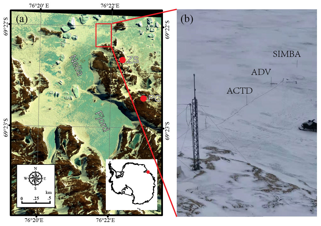
Figure 1 (a) False-colour satellite image of the observation site in Nella Fjord near Zhongshan Station, modified from the WorldView-2 multi-band image taken on 20 October 2012 (https://worldview.earthdata.nasa.gov, last access: 25 May 2023). (b) Photo of the observation site taken from a 30 m-high slope on 12 April 2021 by Jinkai Ma, one of the co-authors. The photo is not planar like the red box in panel (a) because of the angle of the shot. The distances between ACTD, ADV, and SIMBA were about 5 m.

From 16 April to 7 November 2021, an integrated ice–ocean interaction observation system was established by the wintering team at the coastal landfast ice site, approximately 1 km from Zhongshan Station (Fig. 1b). A cable-type CTD sensor (ALEC ACTD–DF, Japanese JFE Advantech Co., Ltd., https://www.analyticalsolns.com.au/product/conductivity_temperature_depth_logger_miniature_.html, last access: 24 February 2023) was deployed 2 m beneath the ice surface and 15 m from the shoreline. The CTD measured the ocean conductivity, temperature, and depth at a frequency of 30 s, with accuracies of ±0.02 mS cm⁻¹ (±0.03 psu) for conductivity (salinity) and ±0.02 ^∘C for temperature. An ADV (SonTek Argonaut–ADV, the xylem company, https://www.xylem.com/siteassets/brand/sontek/resources/specification/sontek-argonaut-adv-brochure-s11-02-1119.pdf, last access: 24 February 2023) was deployed to observe the 3-D ocean velocity at 5 m below the ice surface and 5 m north of the CTD. The frequency of the ocean velocity observations was 40 s, and the accuracy was ±0.001 m s⁻¹. A SIMBA (SRSL SIMBA, SAMS Enterprise Ltd., https://www.sams-enterprise.com/services/autonomous-ice-measurement/, last access: 24 February 2023) was deployed 5 m north of the ADV, which contained 240 temperature sensors at 2 cm intervals mounted on a thermistor string. The 4.8 m-long SIMBA temperature chains recorded the vertical temperature profiles of air–snow–ice–ocean every 6 h. The SIMBA had a resolution of ±0.0625 ^∘C. The water depths at the CTD, ADV, and SIMBA sites were 4.5, 13, and 13 m, respectively. Manual observations, including snow and ice thickness measurements, were conducted around the integrated ice–ocean interaction observation system every 5 d by the wintering team.

Due to the effect of the extremely cold conditions on the battery power supply, the observation system stopped working during part of the period, 24 April–11 May for the ADV and 7–15 July for the CTD. A data quality control was applied to the original time series to pick out the anomalous values. To match the different frequencies of the ADV and CTD in the inter-comparisons and the analysis of the oceanic heat flux, the observations were averaged and integrated into a new time series with 2 min intervals. Regarding the processing of the SIMBA observation data, three-point smoothing was introduced to minimize the noise influences, which has been used by Zhao et al. (2017) and Tian et al. (2017).

2.2 Satellite and reanalysis products

To further investigate the large-scale influences, satellite and reanalysis products were used. The Advanced Microwave Scanning Radiometer 2 (AMSR2) sea ice concentration based on the Arctic Radiation and Turbulence Interaction Study (ARTIST) sea ice (ASI) algorithm developed at the University of Bremen (https://seaice.uni-bremen.de/sea-ice-concentration/amsre-amsr2/, last access: 24 February 2023) was adopted to obtain the percentage of open water in Prydz Bay. These data are updated daily and have a spatial resolution of 6.25 km (Spreen et al., 2008). The Operational Mercator global ocean reanalysis products, produced by the Copernicus Marine Environment Monitoring Service (CMEMS), provide the daily and monthly ocean currents and mixed-layer depth of the global ocean with a 1/12^∘ spatial resolution and 3 h frequency (for more information, see https://doi.org/10.48670/moi-00016, last access: 24 February 2023) for a large-scale analysis. To facilitate comparative analysis, in this study, the nearest-neighbour method was employed to interpolate the CMEMS products to the same projection and spatial resolution as the AMSR2 sea ice concentration.

2.3 Oceanic heat flux estimation methods

2.3.1 Residual method

The residual method was adapted from the classical Stefan law. By obtaining measurements of the ice vertical temperature profiles and ice bottom growth or ablation, the residual method has been widely used to estimate the oceanic heat fluxes in previous studies (McPhee and Untersteiner, 1982; Lytle et al., 2000; Perovich and Elder, 2002; Purdie et al., 2006; Lei et al., 2010; Zhao et al., 2019). At the bottom of the sea ice, the heat balance can be expressed by an equilibrium equation as follows:

$$\begin{array}{}\text{(1)}& F_w=F_{\mathrm{c}}+F_{\mathrm{l}}+F_{\mathrm{s}},\end{array}$$

where F_w is the heat flux from the ocean to the sea ice, F_c is the heat conduction flux through the sea ice, F_l is the latent heat flux caused by the freezing or melting of the ice, and F_s is the specific heat flux generated by the change in the ice temperature. In Eq. (1), the signs of the melting, heating, and upward heat flow are positive, while the signs of the cooling, freezing, and downward heat flow are negative.

The three heat flux terms can be further expressed as follows (Semtner, 1976; Lei et al., 2014):

$$\begin{array}{}\text{(2)}& {\displaystyle }{F}_{\mathrm{c}}=k_{\mathrm{i}}{\displaystyle \frac{T_{\mathrm{0}}-T_{\mathrm{f}}}{H}},\text{(3)}& {\displaystyle }{F}_{\mathrm{l}}=-{\mathit{\rho }}_{\mathrm{i}}{L}_{\mathrm{i}}{\displaystyle \frac{\mathrm{d}H}{\mathrm{d}t}},\text{(4)}& {\displaystyle }{F}_{\mathrm{s}}={\mathit{\rho }}_{\mathrm{i}}{c}_{\mathrm{i}}\mathrm{\Delta }H{\displaystyle \frac{\mathrm{d}T}{\mathrm{d}t}},\end{array}$$

where k_i is the thermal conductivity of the sea ice, T₀ is the temperature of the ice in the reference layer (details are provided in Sect. 3.4), H is the corresponding sea ice thickness, T_f is the freezing point, ρ_i is the density of the ice, L_i and c_i are the latent and specific heat capacities of the sea ice, ΔH is the sea ice thickness of the reference layer, $\mathrm{d}H/\mathrm{d}t$ is the ice growth rate, and $\mathrm{d}T/\mathrm{d}t$ is the change in the sea ice temperature (Untersteiner, 1961; Millero, 1978; McPhee and Untersteiner, 1982; Lei et al., 2010). The density and salinity of the landfast ice used in this study were 910 kg m⁻³ and 4 psu based on previous observations reported by Lei et al. (2010). k_i, L_i, and c_i are functions of the salinity and temperature of the ice, and T_f is a function of seawater salinity. These parameters were re-estimated based on the CTD observations. The vertical ice temperature gradient, ice growth/melt rate, and ice temperature changes were calculated from the SIMBA observations.

2.3.2 Bulk parameterization method

The oceanic heat flux can be determined from direct measurements of the high-frequency current velocity, temperature, and salinity in the mixed layer in the upper ocean beneath the ice cover in order to evaluate the turbulent heat flux at the ice–ocean interface, which is called the turbulent parameterization method (McPhee, 1992; McPhee et al., 2008). The oceanic heat flux F_w from the ocean mixed layer to the bottom of the sea ice can be expressed as follows (Guo et al., 2015):

$$\begin{array}{}\text{(5)}& F_w={\mathit{\rho }}_w{c}_w\langle w^{\prime }{T}^{\prime }\rangle ,\end{array}$$

where ρ_w and c_w are the density and specific heat capacity of the ocean mixed layer and $\langle w^{\prime }{T}^{\prime }\rangle$ is the turbulent heat flux. The heat transferred from the ocean to the ice depends on both the turbulent stress at the ice–ocean interface (characterized by the frictional velocity $u_{\mathrm{0}}^{\ast }$ as the square root of the kinetic stress at the interface) and the effective heat content of the fluid in the turbulent boundary layer, which is roughly proportional to the deviation of the ocean temperature above the freezing point (McPhee, 1992; McPhee et al., 1999; Kirillov et al., 2015). Therefore, the turbulent heat flux can be further parameterized as follows:

$$\begin{array}{}\text{(6)}& \langle w^{\prime }{T}^{\prime }\rangle =c_{\mathrm{H}}{u}_{\mathrm{0}}^{\ast }\mathrm{\Delta }T,\end{array}$$

where c_H is the Stanton number of heat exchange efficiency, ΔT is usually expressed as the difference between the ocean temperature and the freezing point, and $u_{\mathrm{0}}^{\ast }$ is the friction velocity at the interface. For the boundary layer beneath the sea ice, the Stanton number c_H is usually assumed to be a constant value of 0.0057 (McPhee, 2002). Therefore, Eq. (5) can be expressed as follows:

$$\begin{array}{}\text{(7)}& F_w={\mathit{\rho }}_w{c}_w{c}_{\mathrm{H}}{u}_{\mathrm{0}}^{\ast }\mathrm{\Delta }T.\end{array}$$

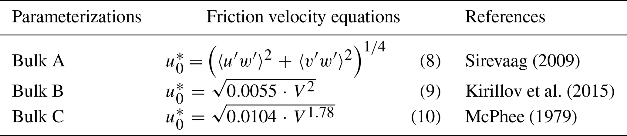
Owing to the roughness beneath sea ice and the fact that the data lack an ocean velocity profile, the friction velocity $u_{\mathrm{0}}^{\ast }$ is usually parameterized using the law of quadratic resistance related to the free-stream current. In this study, three different bulk parameterization methods were used to estimate the friction velocity (Table 1). V is the absolute flow velocity relative to the motionless landfast ice, which was observed by the ADV in this study. The velocity perturbations u^′, v^′, and w^′ were estimated by removing the mean from the original time series with 15 min windows.

Table 1 Three different parameterizations of the friction velocity $u_{\mathrm{0}}^{\ast }$.

3 Results

3.1 Snow and ice evolution

Figure 2a shows the SIMBA observations from 16 April to 7 November 2021. The serial numbers of the thermistors start from the deep end of the string in the ocean. Sensor no. 180 represents the initial location of the ice surface on 16 April, when the SIMBA was deployed in the field (dotted lines in Fig. 2). Typically, the sensors above the dotted lines were located in the air and their temperature data exhibited significant daily variations. The sea ice temperature exhibited an obvious gradient of 0.11–0.24 ^∘C cm⁻¹. The ocean temperature was stable, ranging from −1.7 to −1.9 ^∘C, which was close to the freezing point. The bottom of the ice (dashed lines in Fig. 2) was identified through visual interpretation according to the method of Zhao et al. (2017). The ice surface did not experience obvious changes during the cold season, and therefore the changes in the ice thickness mainly occurred at the bottom of the ice. The landfast ice was 44 cm thick on the first observation day (16 April), continued to freeze from May to mid-October, and reached the maximum thickness of 142 cm on 22 October. After this, the bottom of the ice began to melt at a mean rate of −0.4 ± 0.2 cm d⁻¹ until the end of the observation period. The mean growth rate during the study period was 0.5 ± 0.3 cm d⁻¹, and the maximum daily growth rate was 1.6 cm d⁻¹ on 10 May 2021. The monthly mean growth rate was largest in May (0.8 ± 0.4 cm d⁻¹) and smallest in October (0.1 ± 0.2 cm d⁻¹), which is similar to the nearshore observations at Zhongshan Station in 2006 (Lei et al., 2010) and in 2012 (Zhao et al., 2019) but different to the offshore cases around this region, especially when grounded icebergs existed (Li et al., 2023).

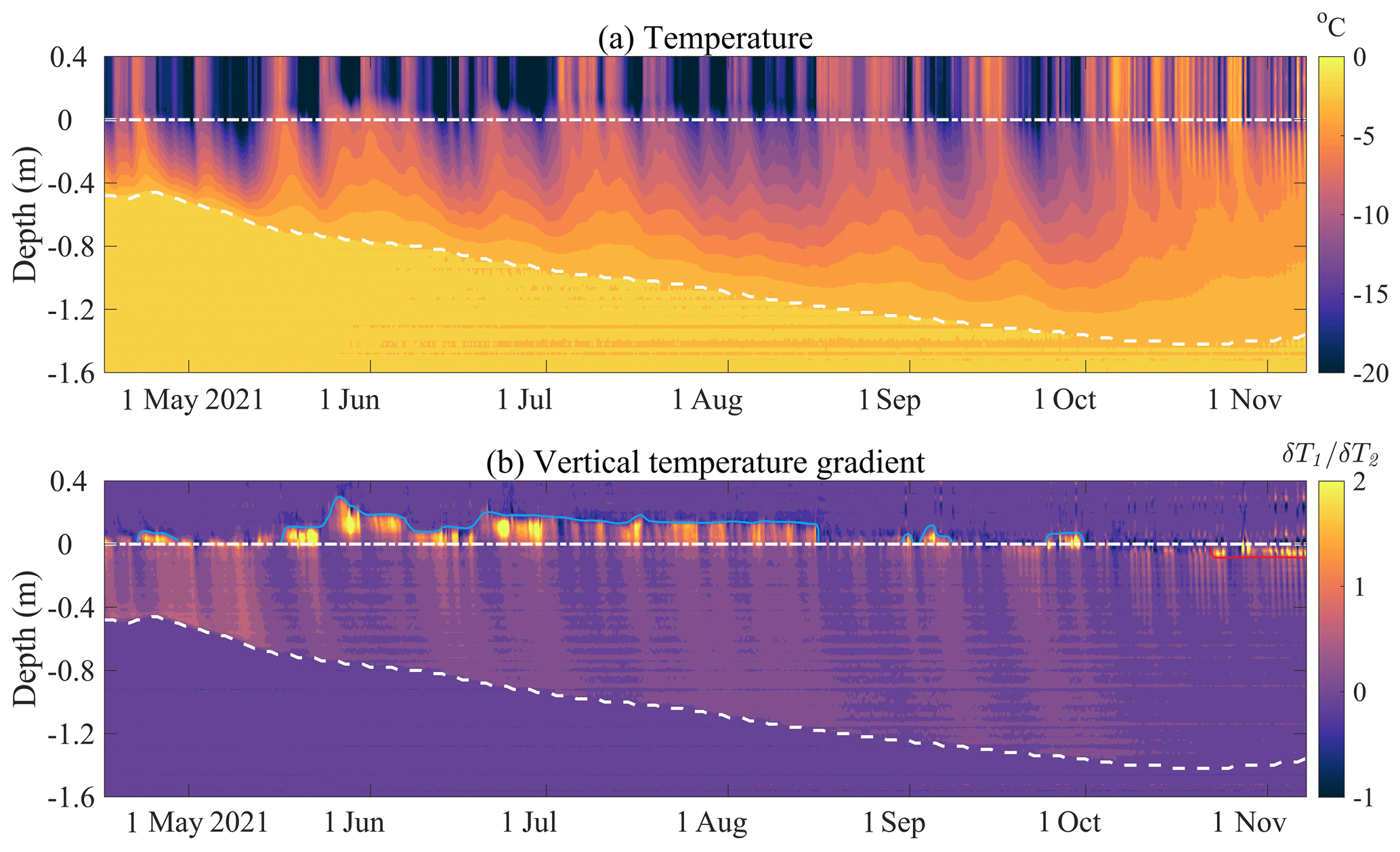
Figure 2 (a) Temperature profiles and (b) vertical gradient of the temperature profiles recorded by the SIMBA every 6 h during April–November 2021. The white dashed line and dotted lines in panels (a) and (b) represent the bottom of the ice and the initial ice surface, respectively. The blue lines and red lines in panel (b) represent the snow surface and new ice surface after sublimation or melting in summer.

The vertical gradient of the ice temperature profiles shows that snow accumulation on top of the ice cover occurred from May to August and experienced discontinuous disappearance due to strong winds after September (thin blue lines in Fig. 2b). Finally, the snow completely disappeared in October, when the air temperature rose up to −2.7 ^∘C. The ice surface began to melt under the strong solar radiation, and 6–8 cm of sublimation was observed by the SIMBA (thin red lines in Fig. 2b). In particular, shortly after the SIMBA was deployed, the landfast ice thickness experienced a 4 cm decrease during 21–26 April, when the warm air reached the observation site in the cold winter and the oceanic heat flux exhibited significant high values during this period.

3.2 Ocean temperature, salinity, and density

The time series of the ocean temperature were observed by the CTD deployed 2 m below the surface of the landfast ice. Figure 3a shows the 194 d high-frequency temperature record with a 2 min interval obtained from 16 April to 6 November 2021. The ocean temperature experienced a rapid increase during 16–23 April from −1.62 to −1.30 ^∘C, and then it gradually decreased to −1.75 ^∘C in the middle of May. In the following months, the ocean temperature remained at around −1.79 ^∘C, with a small standard deviation of 0.01 ^∘C, until the end of the observations. Therefore, the ocean beneath the ice was relatively warm and was highly variable before the middle of May (−1.64 ± 0.10 ^∘C), while the ocean temperature dropped and remained close to the freezing point from then on (−1.79 ± 0.01 ^∘C). Based on the spectral analysis, the time series of the ocean temperature exhibited an obvious half-day period, which may be related to the tidal oscillations.

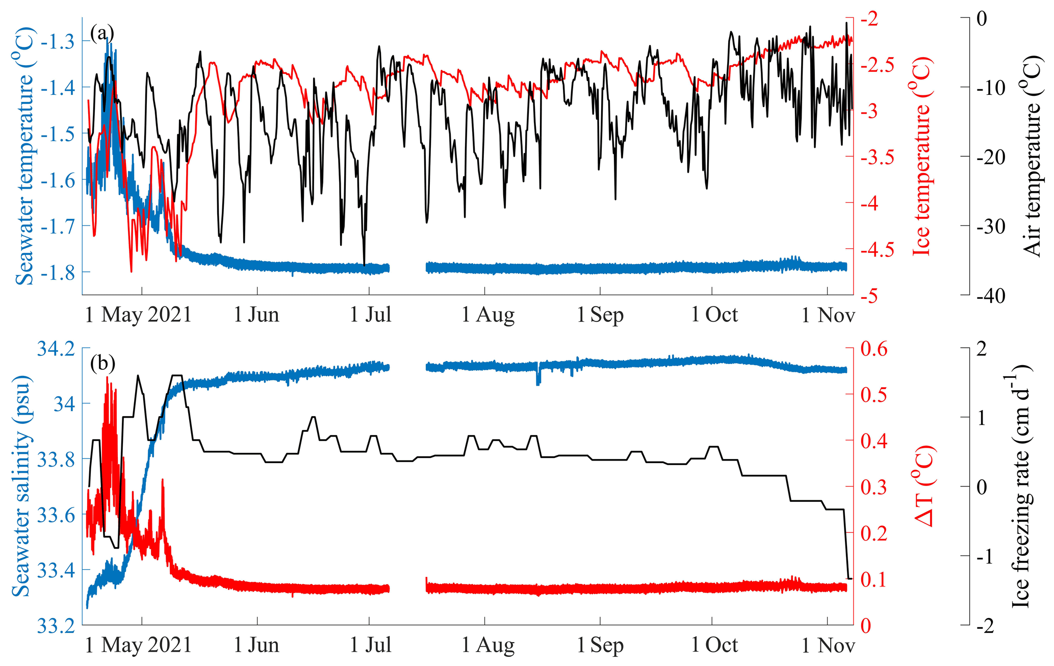
Figure 3 (a) The seawater temperature observed by the CTD at 2 m beneath the landfast ice surface (blue lines), the ice temperature at the bottom (red lines, defined as the mean temperature derived by the SMIBA sensor located 0.1 m above the bottom of the ice), and air temperature observed by the SIMBA at 1 m above the landfast ice surface. (b) The seawater salinity observed by the CTD (blue lines), the deviation of seawater temperature above the freezing point (ΔT, red lines), and the ice freezing rate at the bottom (black lines) observed by the SIMBA from 16 April to 7 November.

The temperature at the bottom of the sea ice (defined as the mean SMIBA sensor temperature in the lowest 10 cm of the sea ice) was lower than the ocean temperature, indicating that heat was transferred from the warm water to the cold sea ice and inhibited ice growth at the bottom of the ice. During April–May, the temperature at the bottom of the sea ice exhibited large variations (−5 to −2.5 ^∘C) in response to the variations in the air temperature when the ice was thin and nearly no snow existed. After the thick snow cover formed, the temperature at the bottom of the sea ice became steady (−2 to −3 ^∘C) from June to November, and the ocean temperature remained stable at around −1.8 ^∘C. In particular, the SIMBA recorded a basal ice melting of 4 cm during 16–26 April. This event was accompanied by a concurrent increase in both the air temperature and ocean temperature, suggesting a heightened transfer of heat from both the air and ocean to the sea ice.

The seawater salinity experienced a rapid increase from 33.34 psu in April to 34.08 psu in May, which was related to the salt rejection process caused by the high freezing rate of 1.1 ± 0.3 cm d⁻¹ at the bottom of the ice (Fig. 3b). More specifically, from 19 to 23 April, the seawater salinity experienced a short period of decrease, different from the long and quickly increasing trend, which may have been related to the slowdown of the freezing at the bottom of the ice during this period due to the obvious warming of the air and ocean (Fig. 3a). From then on, the seawater salinity (around 34.13 ± 0.02 psu) largely remained stable with small daily and seasonal deviations. This corresponded to the occurrence of a relatively large and stable freezing rate at the bottom of the ice (around 0.5 ± 0.2 cm d⁻¹) until the middle of October. When the warm season began, the bottom of the sea ice started to melt at a mean rate of −0.4 ± 0.3 cm d⁻¹ (from the middle of October to the middle of November), and the seawater salinity slightly decreased, indicating that the salt rejection became weaker.

As a function of the seawater temperature and salinity, the seawater density was calculated using the observations measured by the CTD and the equation proposed by Millero and Poisson (1981). The seawater density exhibited a trend similar to that of the seawater salinity, which increased significantly during the early winter, with a mean trend of 0.03 kg m⁻³ d⁻¹. In the following observation period, the seawater density was stable, with a mean value of 1027.5 ± 0.02 kg m⁻³.

After acquiring the seawater salinity by CTD, the seawater freezing point was calculated with the observed seawater temperature and salinity using the equation proposed by Millero (1978). The calculated freezing point decreases with the increase in the seawater salinity, from −1.83 ^∘C in April to −1.86 ^∘C in May, and then remained stable, with a mean value of −1.87 ^∘C in the following seasons. Furthermore, the deviation of seawater temperature above the freezing point was calculated (ΔT, red lines in Fig. 3b), which increased quickly from 0.15 to 0.55 ^∘C in April and decreased to around 0.1 ^∘C in the middle of May and remained constant to November.

3.3 Ocean current

The 3-D current velocity in the meridional (U), zonal (V), and vertical (W) directions at 5 m beneath the surface of the landfast ice was obtained by the ADV every 40 s. A rose diagram of the 2 min records of the horizontal current is shown in Fig. 4. The 2 min frequency records of U and V exhibited large oscillations, mainly varying within ±20 cm s⁻¹. In particular, 97 % of the U values and 96 % of the V values were within ±10 cm s⁻¹. W exhibited relatively small oscillations, mainly within ±4 cm s⁻¹, and 98 % of the W values were within ±2 cm s⁻¹. The typical periods of U, V, and W were all half-day periods.

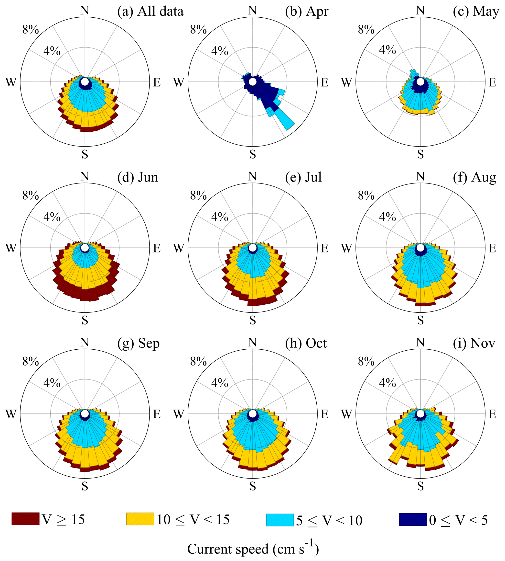
Figure 4 Rose diagram of the horizontal current speed with a 2 min resolution for (a) the total time series and (b–i) different months. The different colours represent the different ranges of the current speed. Due to technical issues, only 8 d were available in April and 20 d in May.

The domain direction was ESE (120^∘)–WSW (240^∘), and 79 % of the velocity measurements were within 5–15 cm s⁻¹ (Fig. 4a). The horizontal velocity was relatively small in April, less than 10 cm s⁻¹, and it gradually increased to the maximum value in June, when 75 % of the velocity measurements were greater than 10 cm s⁻¹. From then on, the horizontal current exhibited a similar distribution in the directions, while the range of the dominant velocity changed from 10–15 to 5–10 cm s⁻¹ (Fig. 4b–i). The horizontal speed exhibited a mean velocity of 9.5 ± 3.9 cm s⁻¹ and a maximum velocity of 29.8 cm s⁻¹ for the 2 min interval records.

3.4 Oceanic heat flux

In the residual method, the vertical gradient of the sea ice temperature is a key term for calculating the conductive heat flux (F_c). Under cold and snow-free conditions, the surface air temperature and freezing point are usually used to calculate the vertical gradient (Lei et al., 2010; Zhao et al., 2019). However, in thick snow or warm cases, the vertical temperature profile of the sea ice is not linear. In this study, a reference layer close to the bottom of the ice was used to calculate the vertical gradient to avoid non-linear biases. McPhee and Untersteiner (1982) set the reference layer at 0.4 m above the bottom of the ice. Perovich and Elder (2002) set the reference layer at 0.4–0.8 m above the bottom of the ice for different ice thickness conditions. Lei et al. (2014) set the reference layer at 0.4–0.7 m above the bottom of the ice. In this study, we defined the reference layer as 0.2 m above the bottom of the ice, and the mean vertical gradient was calculated using the 2 cm interval temperature profile obtained by the SIMBA.

In previous studies, the empirical value of the freezing point was usually used, but a practical value is more realistic in the F_l calculation. Based on the seawater salinity observations recorded by the CTD, the freezing points were estimated following the equation derived by Millero (1978). During the observation period, the freezing point was around −1.83 ^∘C in April, gradually decreased to −1.87 ^∘C in June, and remained at this value until November.

Figure 5 shows the heat fluxes calculated using the residual method. The variation in the latent heat flux (F_l) was strongly correlated with the growth and ablation of the sea ice. During the study period, F_l was negative in the cold season, except for a short melting period in April. During 21–24 April, due to the influences of the warm air and ocean, the SIMBA recorded obvious melting at the bottom of the ice and F_l exhibited a positive value of 20 W m⁻². In October, the melt season began and F_l became positive. The specific heat flux F_s was smaller throughout the study period, oscillating around 0 W m⁻². The conductive heat flux F_c was relatively large before the middle of May (up to 80 W m⁻²), gradually decreased to 20 W m⁻² in September, and finally reached 10 W m⁻² in October and November. The oceanic heat flux exhibited a larger value of 41.3 ± 9.8 W m⁻² in April and then decreased to around 10 W m⁻² from June to October, but it quickly increased to 50 W m⁻² in November before the observation period ended. The mean oceanic heat flux for the entire study period was 12.2 ± 10.9 W m⁻².

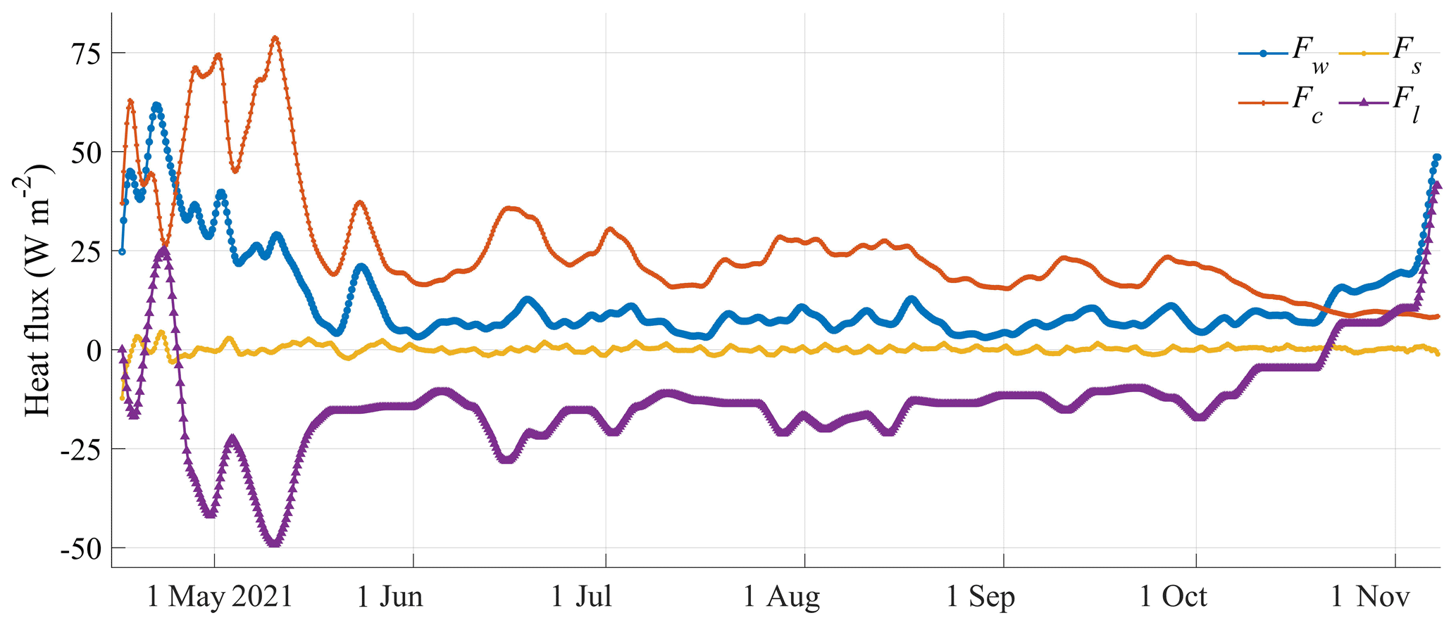
Figure 5 Conductive heat flux (F_c), latent heat flux (F_l), specific heat flux (F_s), and oceanic heat flux (F_w) were estimated using the residual method and a reference layer located 0.2 m above the bottom of the ice. The time interval is 6 h.

In contrast to the residual method, previous studies have developed bulk parameterization methods for calculating the oceanic heat flux when the observations of ocean parameters are available (McPhee, 1979, 1992; Sirevaag, 2009; Kirillov et al., 2015). In this study, the ocean velocity, temperature, and salinity in the ice–ocean boundary layer were recorded at a high frequency by the ADV and CTD, which provided a chance to evaluate the oceanic heat flux using bulk parameterization methods.

During the observation period, the ocean temperature was always warmer than the freezing point, indicating that the heat flux was from the ocean to the ice. The temperature difference (ΔT) between the ocean and the freezing point was 0.26 ± 0.08 ^∘C in April and decreased gradually to 0.08 ^∘C from June to November. Three different bulk parameterization methods were used in this study (Bulk A: Sirevaag, 2009; Bulk B: Kirillov et al., 2015; Bulk C: McPhee, 1979), and their main differences were due to the expressions of the fractional velocity and empirical parameters (Table 1).

The hourly oceanic heat flux values calculated using three bulk parameterization methods exhibit variations similar to those of the results of the residual method, that is, high values of 60–80 W m⁻² in April and then gradually decreasing to 10–30 W m⁻². The mean oceanic heat flux values during the study period were 19.7 ± 5.3 W m⁻², 13.6 ± 3.1 W m⁻², and 24.4 ± 5.4 W m⁻² for the Bulk A, Bulk B, and Bulk C methods, respectively, and 12.2 ± 10.9 W m⁻² for the residual method (Fig. 6a). The values obtained using the bulk methods were 9.0 ± 8.9 W m⁻² larger on average than that obtained using the residual method during the study period.

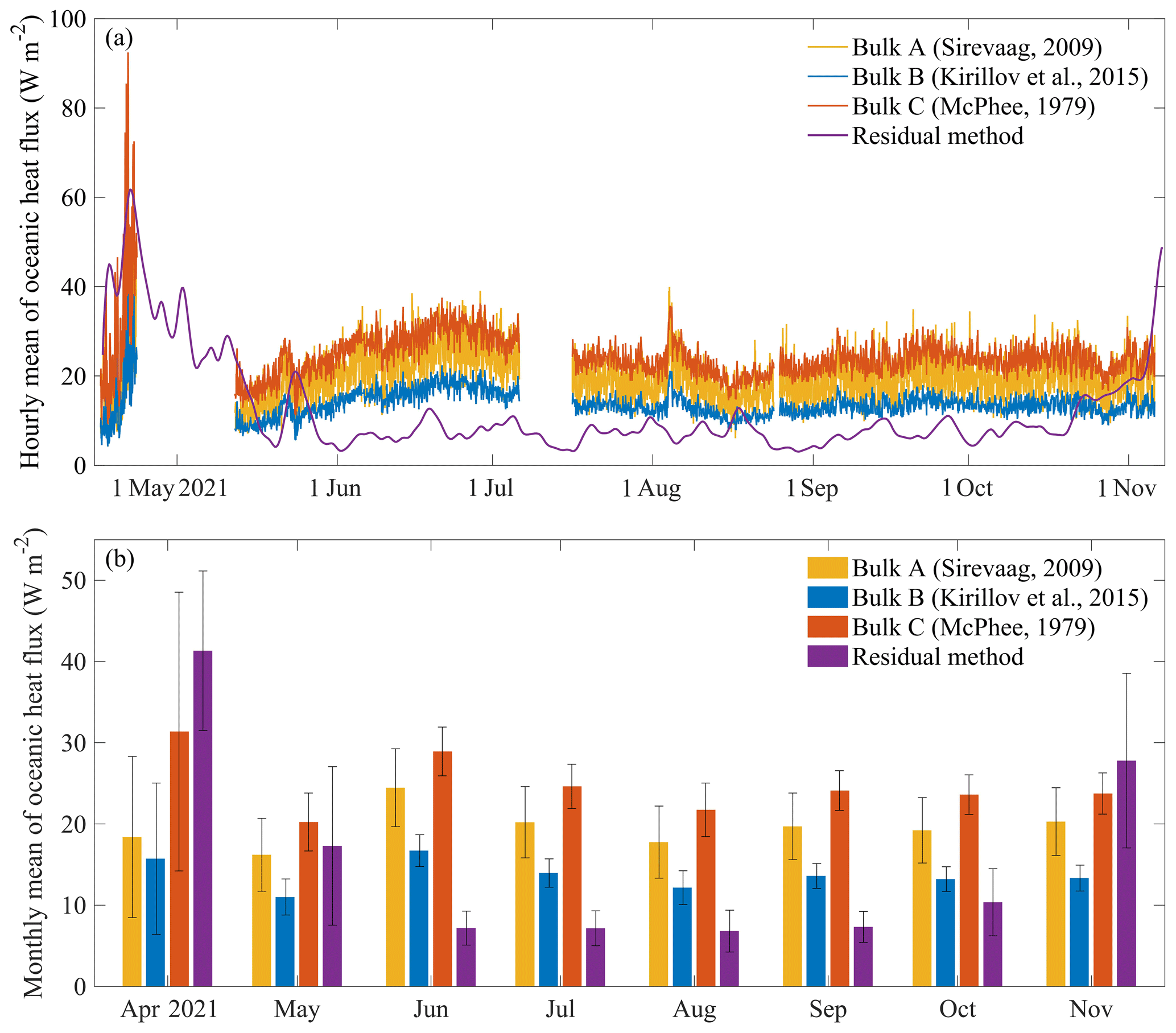
Figure 6 (a) Hourly mean F_w was calculated using the three bulk parameterization methods and the 6-hourly mean F_w was calculated using the residual method and (b) the monthly mean F_w. The error bars in panel (b) represent ±1 standard deviation of the hourly mean values.

According to the monthly oceanic heat flux trends shown in Fig. 6b, the oceanic heat flux values were 18.4, 15.7, 31.4, and 41.3 W m⁻² in April for the Bulk A, Bulk B, Bulk C, and residual methods, respectively. In addition, the oceanic heat flux had large standard deviations in April, 10–20 W m⁻² for the bulk methods and 10 W m⁻² for the residual method, indicating a large variation in the hourly time series. From May to October, the standard deviations were generally less than 5 W m⁻². Among the three bulk parameterization methods, the results of the Bulk C method were relatively larger than those of the Bulk A and B methods.

Previous studies estimated the oceanic heat flux under landfast ice in Prydz Bay using different methods. Allison (1981) estimated the oceanic heat flux near Mawson Station from monthly mean temperature and ice growth data. In the early stage of sea ice growth, the thermohaline convection caused by the brine rejection made the flux very high, and it could reach 50 W m⁻². Heil et al. (1996) used a multi-layer thermodynamic model to simulate sea ice growth at Mawson Station. The multi-year average oceanic heat flux estimated from daily values was 7.9 W m⁻², and the annual mean was 5–12 W m⁻² from 1958 to 1986. Lei et al. (2010) estimated the oceanic heat flux near Zhongshan Station in early April to be 15–20 W m⁻². Yang et al. (2016) estimated the oceanic heat flux to be 25 W m⁻² in March–April using a thermodynamic model. According to weekly observations near Zhongshan Station, Zhao et al. (2019) interpolated and calculated the daily oceanic heat flux from March to May to be 30 W m⁻². In this study, the average oceanic heat fluxes calculated using the residual method and the bulk methods are consistent with those of previous studies on the seasonal scale, and the quantitative difference may be related to the specific methods and environmental parameters for the given years. Compared to the higher temporal resolution (6 h for the residual method and 2 min for the bulk methods) in this study, the estimation based on the traditional borehole observations may produce great errors within a short time window (Lei et al., 2010). Therefore, this high-frequency observation can more accurately capture the subtle changes in oceanic heat flux in the short term and better analyse the annual evolution of the ice–ocean interaction.

4 Discussion

The cross-seasonal minute-frequency observations of variables in the ice–ocean interface in this study provide a clear picture of how they varied on an hourly, daily, or seasonal scale and fill the knowledge gap at Zhongshan Station. Like the related studies in other regions, those variables may be affected by the short-term cycle of the sub-glacial current (McPhee et al., 1996) and ocean tide current (Lei et al., 2010). To further enrich our analysis, the relationships between processes on the local scale and pan-Prydz Bay scale were discussed here.

4.1 Potential influences of local tidal oscillations

The local tides may influence the evolution of sea ice (Lei et al., 2009). The tidal oscillations were reconstructed using the harmonic analysis method (Pan et al., 2018) and the harmonic constants from E et al. (2013). In this study, the periodogram method (Welch, 1967) was used to detect the periodicity of the long time-series observation data. Power spectrum analysis of the signal revealed that the tidal oscillations exhibited two peaks. The largest peak had a period of 1 d, and the second-largest peak had a half-day period, indicating that the tide near Zhongshan Station was an irregular diurnal tide (Fig. 7). To further investigate the relationships between the tidal oscillations and oceanic variables, the same spectral analysis was employed for all of the observed ocean variables. The ocean temperature exhibited the largest peak with a period of 1 d and a relatively low peak with a half-day period. In contrast, the seawater salinity, U, V, W, and the results of the three bulk parameterization methods exhibited the largest peak with a half-day period and a relatively low peak with a 1 d period (Fig. 8). The results of the spectral analysis indicate that the ocean temperature, salinity, U, V, W, and oceanic heat flux were greatly affected by the tidal oscillations.

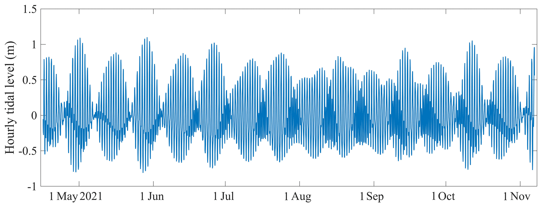
Figure 7 The tidal oscillations were constructed using the harmonic analysis method (Pan et al., 2018) and the harmonic constants of E et al. (2013). The temporal resolution of this dataset is 1 h.

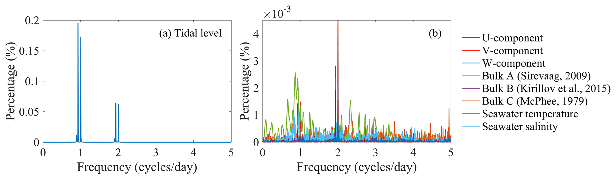
Figure 8 (a) The results of the spectral analysis of the tidal oscillations and the observed ocean variables, and (b) the calculated F_w. The periodogram method was used to detect the periodicity (Welch, 1967).

In April, the observed seawater temperature and salinity exhibited a special pattern; that is, the water was relatively warm and fresh in the equilibrium tide state, while it was cold and salty in the low and high tide states (Fig. 9a, b), which may have been related to the efficient horizontal heat transport when the surrounding area was not completely covered by ice. However, in the other months, the larger observed vertical velocity enhanced the vertical mixing, and therefore no significant variations in the seawater temperature and salinity and the oceanic heat flux were observed during the same period.

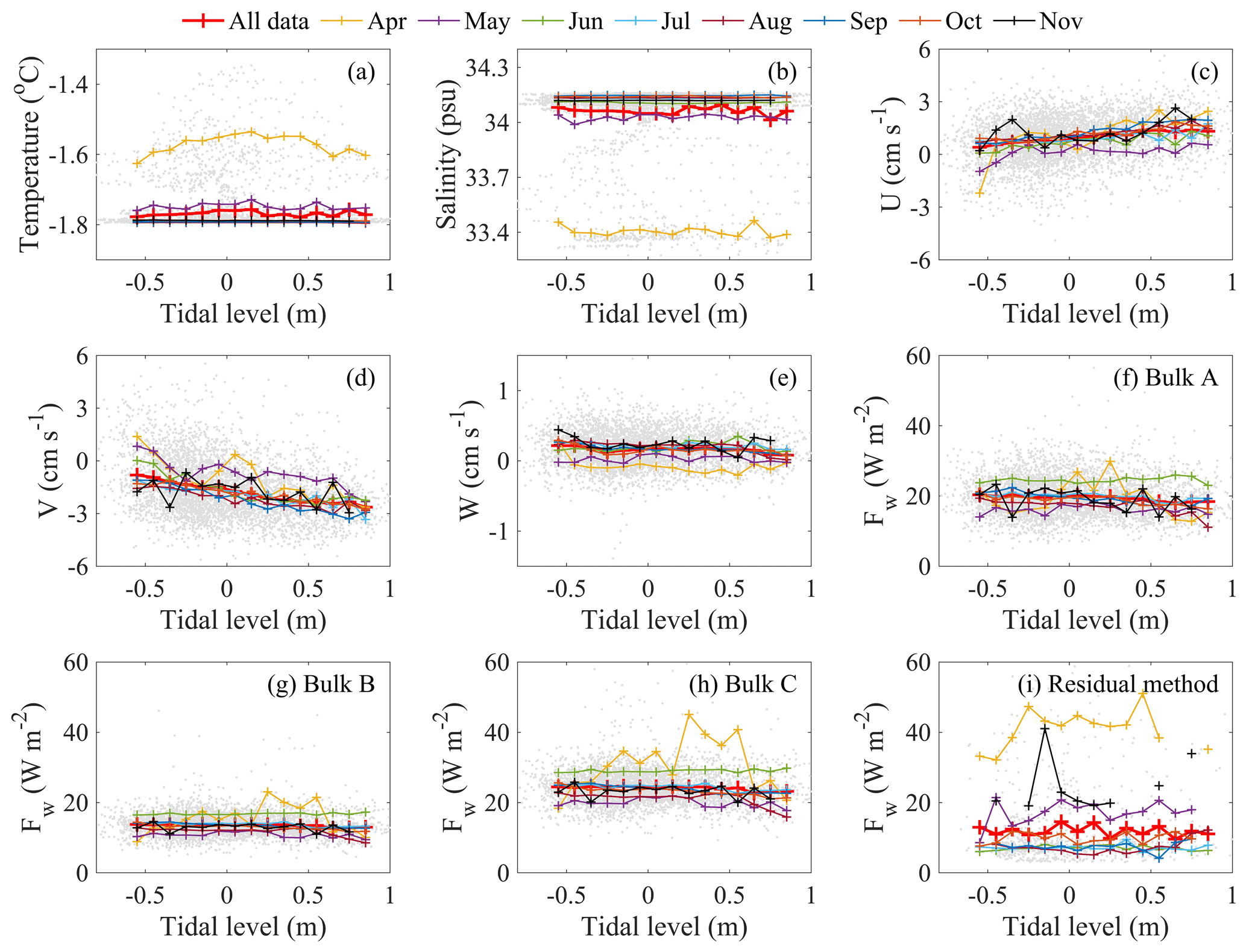
Figure 9 Scatter plots of the tidal level versus the oceanic variables: (a) seawater temperature, (b) seawater salinity, (c) U-component velocity, (d) V-component velocity, (e) W-component velocity, and (f–i) F_w from the Bulk A, B, C, and residual methods. The grey dots are the hourly mean values of the variables, and the different lines represent the monthly mean values for 0.1 m tidal-level bins.

Furthermore, when the tide level changed from low to high, the hourly U changed from a slightly positive distribution (0.7 ± 1.2 cm s⁻¹) to a deeply positive distribution (1.2 ± 1.1 cm s⁻¹), indicating predominantly eastward flow during the high-tide-level conditions (Fig. 9c). V changed from a slightly negative distribution (−1.3 ± 1.6 cm s⁻¹) to an intensely negative distribution (−2.1 ± 1.3 cm s⁻¹), suggesting that the southward flow became stronger when the tide level was high (Fig. 9d). W did not vary prominently, and the mean values were almost the same, 0.2 ± 0.3 cm s⁻¹ and 0.2 ± 0.2 cm s⁻¹ during the low and high tide levels, respectively (Fig. 9e).

4.2 Relationships between large-scale and local phenomena

Prydz Bay was covered by sea ice in the cold season. Ice floes appeared widely in March, and landfast ice started to form 1 month later in April near Zhongshan Station. From May to October, ice floes completely covered Prydz Bay, except for several large polynyas (Fig. 10d), e.g. Davis Polynya (DaP) and Four Ladies Bank Polynya (FLBP) on the eastern side and Mackenzie Bay Polynya (MBP) and Cape Darnley Polynya (CDP) on the western side (Hou and Shi, 2021; Nihashi and Ohshima, 2015; Williams et al., 2016). In addition, the landfast ice gradually extended to around 100 km along the zonal direction. In November, the ice floe concentration decreased, and the landfast ice cover reached the maximum extent (Fig. 10). The open water area accounted for nearly 80 % of the entire ocean grid in March, allowing more solar heat flux to be absorbed by the ocean, which was the energy basis for the warm ocean in April (Fig. 11). The large-scale circulation in Prydz Bay indicated the existence of a westward current along the Antarctic coastline, which was stronger in the ice-free and low-ice-concentration months and weaker in the high-ice-concentration months. In April, the large-scale current carried the warm water from low latitudes to high latitudes, contributing to the observed rise in the ocean temperature near Zhongshan Station. From then on, the large-scale current weakened, and the horizontal heat transport decreased.

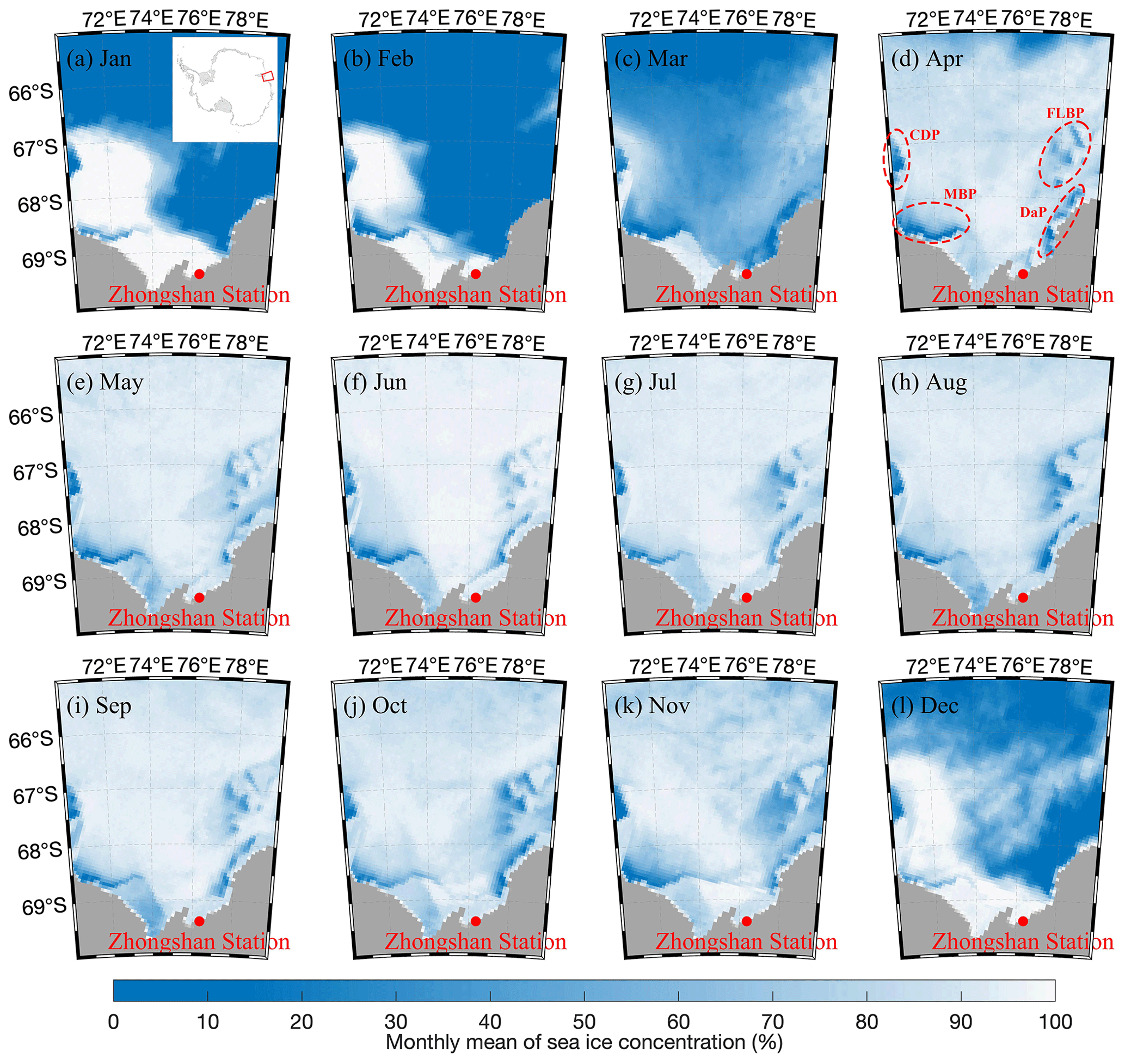
Figure 10 (a–i) Evolution of the monthly sea ice concentration in Prydz Bay from January to December 2021. The domain of Prydz Bay (70–80^∘ E, 65–70^∘ S) in Antarctica is shown in the top-right corner of panel (a). The sea ice concentration dataset was retrieved from the AMSR2 product provided by Bremen University (https://seaice.uni-bremen.de, last access: 24 February 2023), with a spatial resolution of 6.25 km. The locations of four large polynyas are marked in panel (d), i.e. the Davis Polynya (DaP) and Four Ladies Bank Polynya (FLBP) on the eastern side and the Mackenzie Bay Polynya (MBP) and Cape Darnley Polynya (CDP) on the western side.

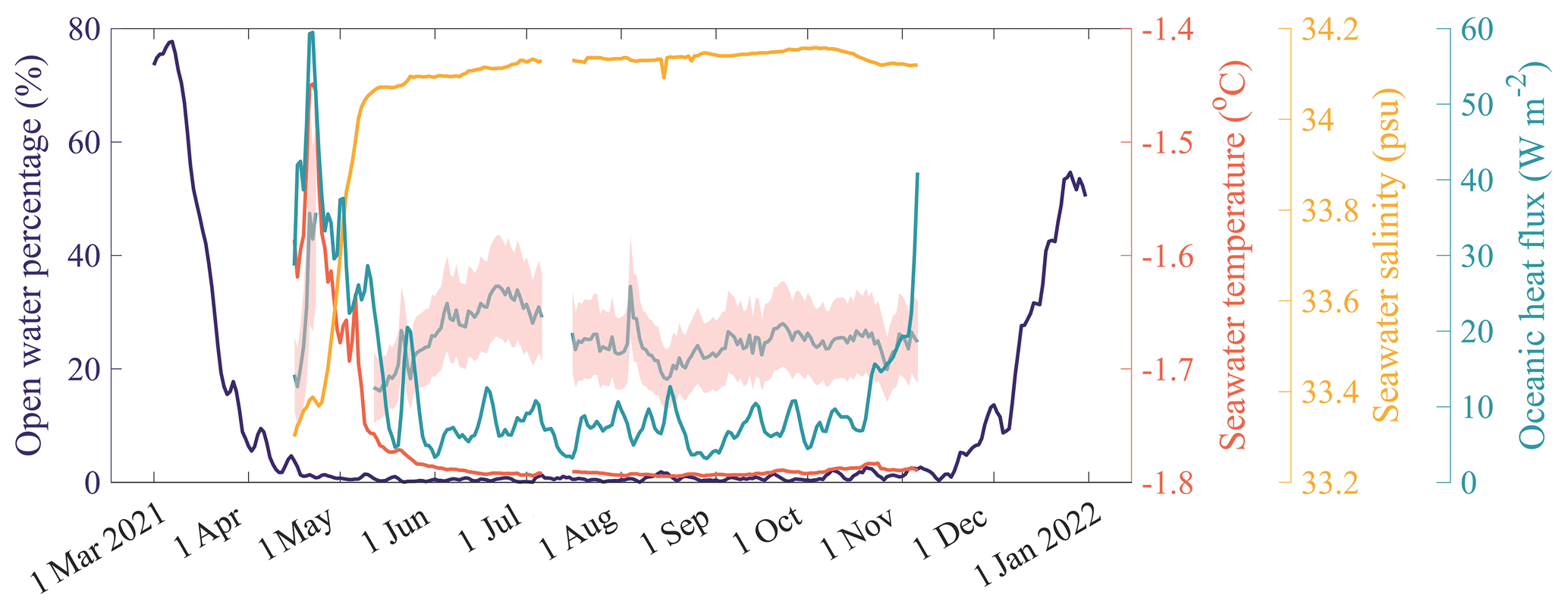
Figure 11 The time series of the daily percentage of open water (purple lines) relative to the domain of Prydz Bay (shown in Fig. 10) and the seawater temperature (red lines), seawater salinity (yellow lines), mean oceanic heat flux from the Bulk A, B, and C methods (grey lines with rose shading), and the oceanic heat flux from the residual method (green lines). The open water area was defined as the sum of the grid cells where the sea ice concentration was less than 15 %. The rose shading indicates ±1 standard deviation.

The four large polynyas shown in Fig. 10d started to form in April, which led to the release of a large amount of salt through new ice production during their existence. As a result, the ocean mixed layer in the corresponding locations derived from Mercator global ocean reanalysis products exhibited obvious thickening from May to October (figure not shown). In addition, the thickening of the entire ice region in Prydz Bay contributed to the strengthened vertical mixing caused by the salt rejection as the sea ice continued to grow. The high seawater salinity observed by the CTD near Zhongshan Station (yellow lines in Fig. 11) confirms this assumption. Considering the reduced horizontal heat transport, the evolution of the ocean temperature was mainly affected by local factors. In this study, the observations were conducted close to the shore at a water depth of around 10 m, making full mixing of the shallow water possible. Therefore, the seawater temperature remained at a stable level from June to November (red lines in Fig. 11).

The water depth near the shoreline may have affected the vertical mixing capacity. The observations of the seawater temperature from the SIMBA sensors at 2 m beneath the ice surface and the CTD were obviously different (mean difference of −0.17 ± 0.03 ^∘C), which was largely beyond the errors of the instruments. The water depths of the SIMBA and CTD sensors were 4.5 and 13 m, respectively, and this difference is believed to have caused the different vertical mixing strengths and thus the different seawater temperatures.

5 Conclusions

The heat and momentum balances among the air, ice, and ocean are some of the most important processes in the polar regions. The air–ice interactions have been well investigated due to the fact that on-ice observations are relatively easy to conduct. However, the ice–ocean interactions have rarely been studied due to the difficulty and limitations of underwater observations. The oceanic boundary layer beneath sea ice plays an important role in the growth and melting of sea ice. In this study, an integrated ice–ocean observation system, including an ADV, CTD, and SIMBA, was deployed on the landfast ice 1 km from Zhongshan Station in Prydz Bay, East Antarctica. The ocean temperature, salinity, and velocity were observed with a 40 s resolution and an 8-month observation period and were investigated for the first time in this region.

The SIMBA temperature chain recorded the vertical temperature profiles of air–snow–ice–ocean, which were used to estimate the snow and ice thicknesses and oceanic heat flux using the residual method. The results show that 98 cm of landfast ice formed from April to October, with a mean growth rate of 0.5 ± 0.3 cm d⁻¹, and 4 cm melted in November, with a rate of −0.4 ± 0.2 cm d⁻¹ until the observation period ended. Approximately 6–8 cm of surface sublimation was observed in summer. The maximum snow thickness was around 30 cm in May and remained at 10–20 cm until August. The CTD recorded the 40 s resolution seawater temperature and salinity at a depth of 5 m beneath the ice surface. The seawater temperature rapidly increased from −1.62 to −1.30 ^∘C in April and then gradually decreased to −1.75 ^∘C in May. The seawater temperature remained stable from June to November, with a mean of −1.79 ± 0.01 ^∘C. In April, the landfast ice was 44–50 cm thick and the ice surface was snow free; therefore, the variations in the air temperature exerted a larger influence on the ice and seawater temperatures. The significant increases in the air and seawater temperatures led to an increase in the temperature of the bottom of the ice, which contributed to the sudden melting of 4 cm from the bottom of the ice observed by the SIMBA. The thick snow cover from May to August provided an isolation layer for the ice and ocean, which contributed to the stability of the seawater temperature during this period.

The seawater salinity increased from 33.34 in April to 34.08 psu in May, with a rate of 0.04 psu d⁻¹. From June to November, the seawater salinity was stable at around 34.13 ± 0.02 psu. The seawater density calculated from the observed seawater salinity increased from 1026.8 to 1027.4 kg m⁻³ from April to May and remained at 1027.5 ± 0.02 kg m⁻³ from then on. The current velocity was recorded by the ADV from April to November. The analysis of the 2 min resolution time series revealed that 79 % of the ocean velocity values were within 5–15 cm s⁻¹, and the mean values during the study period were 9.5 ± 3.9 cm s⁻¹. The maximum velocity of 29.8 cm s⁻¹ was observed on 25 June 2021. The dominant current direction was ESE (120^∘)–WSW (240^∘). The spectral analysis results suggest typical half-day periods for U, V, and W, which may be related to the tidal oscillations near Zhongshan Station. The meridional velocity V was dominated by the southward flow and became stronger when the tide level was higher.

The oceanic heat flux was estimated using the residual method and three different bulk parameterization methods. The results exhibit a similar peak of 60–80 W m⁻² in April–May and a decreasing trend to a stable level of 10–30 W m⁻² from then on. The mean values were 12.2 ± 10.9 W m⁻², 19.7 ± 5.3 W m⁻², 13.6 ± 3.1 W m⁻², and 24.4 ± 5.4 W m⁻², respectively, for the residual and Bulk A, B, and C methods. The large differences were mainly caused by the different formulas for the friction velocity, indicating the uncertainties of the empirical equations. The estimated results obtained in this study are consistent with those of previous studies, which were usually based on low-frequency ice thickness observations. The oceanic heat fluxes exhibited similar half-day periods, which are also believed to be related to the tidal oscillations.

The observations of seawater temperature, salinity, U, V, and W and the estimation of the seawater density and oceanic heat flux exhibited periods similar to those of the local tidal oscillations, suggesting that the tides were one of the main drivers of the oceanic variations near Zhongshan Station. The large-scale sea ice distribution and current transformation affected the absorption of solar radiation by the upper ocean and the horizontal heat transport, which was another main driver of the oceanic variations near Zhongshan Station. Both the local- and large-scale influences played important roles in the oceanic heat flux and thus the ice–ocean interactions.

In this study, the attainment of high-frequency oceanic measurements provided an opportunity to investigate the details of the ice–ocean interactions beneath landfast ice on the diurnal and seasonal scales. The bulk parameterization was used to estimate the oceanic heat flux near Zhongshan Station, providing more interesting information than the residual method does. The use of more ice and ocean equipment, such as ice radar, ocean temperature chains, and ice thickness gauges, will be considered in the future to fill the remaining data gap.