the Creative Commons Attribution 4.0 License.
the Creative Commons Attribution 4.0 License.
 | 17 Jan 2023
Estimating degree-day factors of snow based on energy flux components
Muhammad Fraz Ismail
Wolfgang Bogacki
Markus Disse
Michael Schäfer
Lothar Kirschbauer
Meltwater from mountainous catchments dominated by snow and ice is a valuable source of fresh water in many regions. At mid-latitudes, seasonal snow cover and glaciers act like a natural reservoir by storing precipitation during winter and releasing it in spring and summer. Snowmelt is usually modelled either by energy balance or by temperature-index approaches. The energy balance approach is process-based and more sophisticated but requires extensive input data, while the temperature-index approach uses the degree-day factor (DDF) as a key parameter to estimate melt of snow and ice merely from air temperature. Despite its simplicity, the temperature-index approach has proved to be a powerful tool for simulating the melt process especially in large and data-scarce catchments.
The present study attempts to quantify the effects of spatial, temporal, and climatic conditions on the DDF of snow in order to gain a better understanding of which influencing factors are decisive under which conditions. The analysis is based on the individual energy flux components; however, formulas for estimating the DDF are presented to account for situations where observed data are limited. A detailed comparison between field-derived and estimated DDF values yields a fair agreement with bias = 0.14 mm ∘C−1 d−1 and root mean square error (RMSE) = 1.12 mm ∘C−1 d−1.
The analysis of the energy balance processes controlling snowmelt indicates that cloud cover and snow albedo under clear sky are the most decisive factors for estimating the DDF of snow. The results of this study further underline that the DDF changes as the melt season progresses and thus also with altitude, since melting conditions arrive later at higher elevations. A brief analysis of the DDF under the influence of climate change shows that the DDFs are expected to decrease when comparing periods of similar degree days, as melt will occur earlier in the year when solar radiation is lower, and albedo is then likely to be higher. Therefore, the DDF cannot be treated as a constant parameter especially when using temperature-index models for forecasting present or predicting future water availability.
- Article
(8698 KB) - Full-text XML
-
Supplement
(774 KB) - BibTeX
- EndNote


Meltwater from snow- and ice-dominated mountainous basins is a main source of fresh water in many regions (Immerzeel et al., 2020). Seasonal snow cover and glaciers act as natural reservoirs which significantly affect catchment hydrology by temporarily storing and releasing water on various timescales (Jansson et al., 2003). In such river basins, snow and glacier melt runoff modelling is a valuable tool when predicting downstream river flow regimes, as well as when assessing the changes in the cryosphere associated with climate change (Hock, 2003; Huss and Hock, 2018). Therefore, a more accurate quantification of the snowmelt and ice melt processes and related parameters is the key to a successful runoff modelling of present and future water availability.
Two different approaches are common in snowmelt modelling. The energy balance approach is process-based but data-intensive, since melt is deduced from the balance of incoming and outgoing energy components (Braithwaite, 1995; Arendt and Sharp, 1999). On the contrary, temperature-index models, also called degree-day models, merely use the air temperature as an index to assess melt rates (Martinec, 1975; Bergström, 1976; Quick and Pipes, 1977; DeWalle and Rango, 2008). The degree-day approach is very common and popular since air temperature is an excellent surrogate variable for the energy available in near-surface atmosphere that governs the snowmelt process (Lang and Braun, 1990). The relationship between temperature and melt is defined by the degree-day factor (DDF) (Zingg, 1951; Braithwaite, 2008), which is the amount of melt that occurs per unit positive degree day (Braithwaite, 1995; Kayastha et al., 2003; Martinec et al., 2008). There are different methods by which the DDF can be determined, e.g. by measurements using ablation stakes (Zhang et al., 2006; Muhammad et al., 2020), by using snow lysimetric outflows (Kustas et al., 1994), by estimating daily changes in the snow water equivalent (Martinec, 1960; Rango and Martinec, 1979, 1995; Kane et al., 1997), or by using satellite-based snow cover data (Asaoka and Kominami, 2013; He et al., 2014).
The DDF is usually treated as a decisive parameter subject to model calibrations because sufficient direct observations are typically lacking in large catchments. Most commonly, for calibrating the DDF, runoff is used (Hinzman and Kane, 1991; Klok et al., 2001; Luo et al., 2013; Bogacki and Ismail, 2016). However, it is also important to note that the calibration of the DDF using runoff can be significantly affected by other model parameters due to their interdependency (Gafurov, 2010; He et al., 2014). Researchers also select DDF directly from other studies; hence, the spatial transferability is not always good (e.g. Carenzo et al., 2009; Wheler, 2009). Despite its simplicity, this approach has proved to be a powerful tool for simulating the complex melt processes especially in large and data-scarce catchments (Zhang et al., 2006; Immerzeel et al., 2009; Tahir et al., 2011; Lutz et al., 2016).
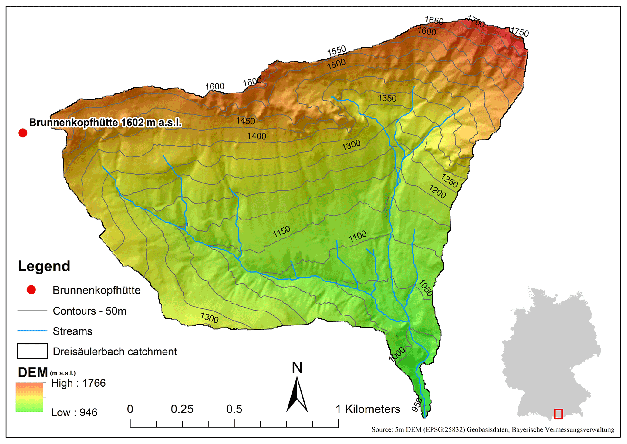
Figure 1Location of the Brunnenkopfhütte automatic snow and weather station in the Dreisäulerbach catchment – German Alps.
Extensive research has been devoted to the enhancement of the original degree-day approach. Braun (1984) introduced the temperature- and wind-index method by the inclusion of a wind-dependent scaling factor. A hybrid approach, which combines both temperature-index and energy balance methods, was introduced by Anderson (1973). Oerlemans (2001) introduced a simplified energy balance approach. Hock (1999) attempted to improve the simple temperature-index model by adding a term to consider potential incoming direct solar radiation for clear-sky conditions. The potential clear-sky solar radiation is calculated as a function of the position of the Sun, geographic location, and a constant atmospheric transmissivity (Hock and Noetzli, 1997; Hock, 1999). This model is comparable with the data requirements of a simple degree-day model. Pellicciotti et al. (2005) considered the net shortwave radiation instead of just incoming shortwave radiation by including snow albedo in their proposed degree-day model. Although all these enhancements focus on adding more physical foundation to the original degree-day method, the classical approach is still more popular because of its simplicity and merely dependence on air temperatures.
A weakness of the degree-day approach is the fact that it works well over longer time periods (e.g. 10 d, monthly, seasonal) but with increasing temporal resolution, in particular for sub-daily time steps, the accuracy decreases (Lang, 1986; Hock, 1999). In addition, the spatial variability of melt rates is not modelled accurately as the DDFs are usually considered invariant in space. However, melt rates can be subject to substantial small-scale variations, particularly in high-mountain regions due to topography (Hock, 1999). For example, topographic features (e.g. topographic shading, aspect, and slope angles) including altitude of a basin can influence the spatial energy conditions for snowmelt and lead to significant variations of the DDF (Hock, 2003; Marsh et al., 2012; Bormann et al., 2014). Under otherwise similar conditions, DDFs are expected to increase with (i) increasing elevation, (ii) increasing direct solar radiation input, and (iii) decreasing albedo (Hock, 2003).
Obviously, the DDF cannot be treated as a constant parameter as it varies due to the changes in the physical properties of the snowpack over the snowmelt season (Rango and Martinec, 1995; Prasad and Roy, 2005; Shea et al., 2009; Martinec et al., 2008; Ismail et al., 2015; Kayastha and Kayastha, 2020). The spatio-temporal variation in the DDF (Zhang et al., 2006; Asaoka and Kominami, 2013) not only affects the accuracy of snowmelt and ice melt modelling (Quick and Pipes, 1977; Braun et al., 1993; Schreider et al., 1997) but is also key to estimating heterogeneity of the snowmelt regime (Hock, 1999, 2003; DeWalle and Rango, 2008; Braithwaite, 2008; Schmid et al., 2012). Since melt depends on energy balance processes and topographic settings, changes in DDFs are a result of energy components that vary with different climatic conditions (Ambach, 1985; Braithwaite, 1995). Another topic that needs attention is the stationarity of the DDF under climate change (Matthews and Hodgkins, 2016). Moreover, it is important to consider the over-sensitivity of temperature-index models, often used by large-scale studies, to future warming (Bolibar et al., 2022; Vincent and Thibert, 2022). Future water availability under climate change scenarios is typically modelled with DDFs calibrated for the present climate, which increases the parametric uncertainty introduced by the hydrological models (Lutz et al., 2016; Ismail and Bogacki, 2018; Hasson et al., 2019; Ismail et al., 2020).
In order to allow for a more-process-based estimate of the DDF, the present study attempts to quantify the contribution of each energy balance component to snowmelt and subsequently to the overall DDF. Considering that degree-day models are typically utilised in large catchments with data-scarce conditions, we estimate energy balance components by formulas with minimum data requirement following the approach by Walter et al. (2005). Based on these formulas, the DDF contribution corresponding to the respective energy components is quantified in tables and graphs for common snowmelt conditions, which can be used for a rapid appraisal. The presented approach is open in the sense that if for any of the energy balance components observed data are available, or more sophisticated models are desired, these can easily replace each of the presented approximations.
The objective of this study is not to incorporate an energy-balance-based DDF approach into temperature-index models but rather to gain a quantitative insight on how different factors affect the DDF. Through this approach, we aim to obtain a good estimate and realistic limits for calibration of the DDF parameter to predict changes during the melt season for forecasting purposes or to study the effects of climate change.
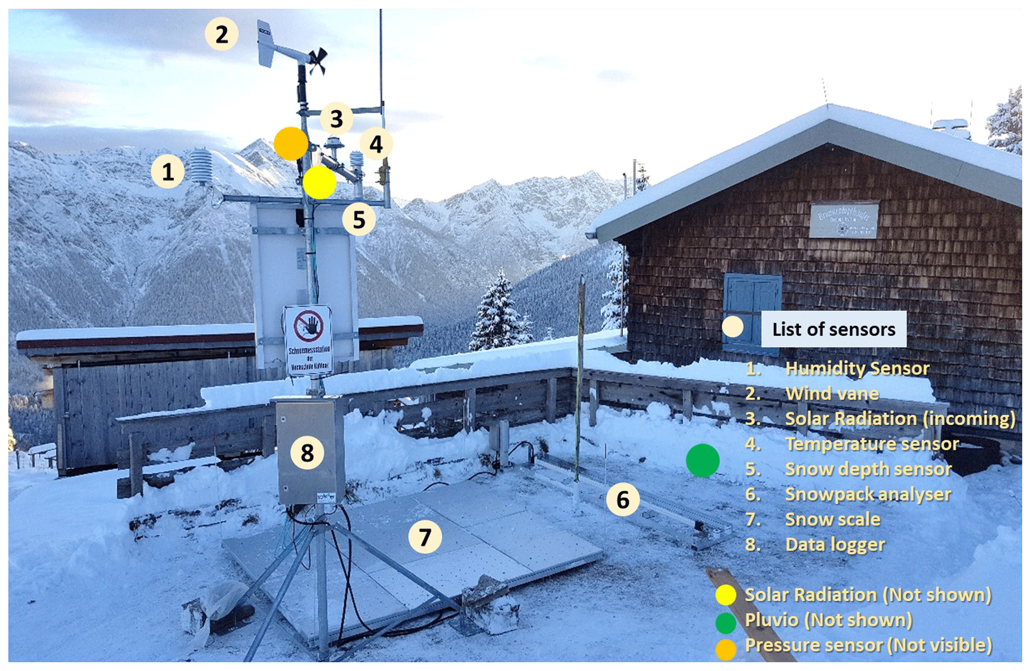
Figure 2Automatic snow and weather station at Brunnenkopfhütte, 1602 m a.s.l. (image credit: Wolfgang Bogacki).
2.1 Test site
The test site is located in the Dreisäulerbach catchment, which is a part of the Isar river system and lies in the sub-alpine region of Bavaria in the Ammergau Alps (Ammergauer Alpen), Germany. The Dreisäulerbach catchment approximately lies between latitudes 47∘34′55′′–47∘35′05′′ N and longitudes 10∘56′40′′–10∘57′07′′ E. It covers an area of about 2.3 km2 and has a mean hypsometric elevation of just over 1200 m a.s.l. (Fig. 1). The elevation ranges from about 950 m a.s.l. at the Linderhof gauging station up to 1768 m a.s.l. at the Hennenkopf station.
The area is mostly characterised by south-facing slopes but also contains northern slopes in southern parts of the catchment. The catchment is densely forested, which during the winter season is fully snow covered. The mean annual temperature in the observation period (i.e. November 2016–May 2021) is about 5.8 ∘C, and the long-term (i.e. 1961–2018) mean annual precipitation at the Ettal-Linderhof station of the Water Science Service Bavaria is reported to be 1676 mm (Kopp et al., 2019).
In order to observe the seasonal snow dynamics, snow measurement instruments in addition to a standard meteorological station have been installed at the Brunnenkopfhütte test site at an elevation of 1602 m a.s.l. (see Fig. 2). The installed station has various sensors that measure temperature, pressure, wind, solar radiation (incoming, outgoing), snow depth, snow scale, a snowpack analyser, and a pluviometer. Table 1 summarises the observed monthly meteorological data at Brunnenkopfhütte station. Figure 3 presents the observed snow water equivalent (SWE) at the test site.
Table 1Observed monthly average meteorological data at Brunnenkopfhütte (November 2016–May 2021).
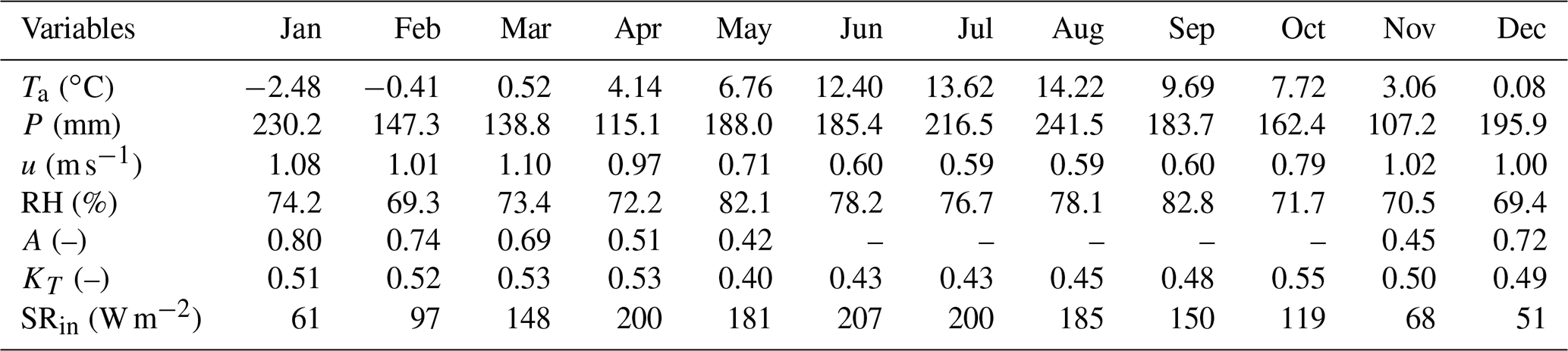
Ta: air temperature; P: precipitation; u: wind speed; RH: relative humidity; A: albedo (only considered when ground is snow covered); KT: clearness index; SRin: incoming shortwave radiation.
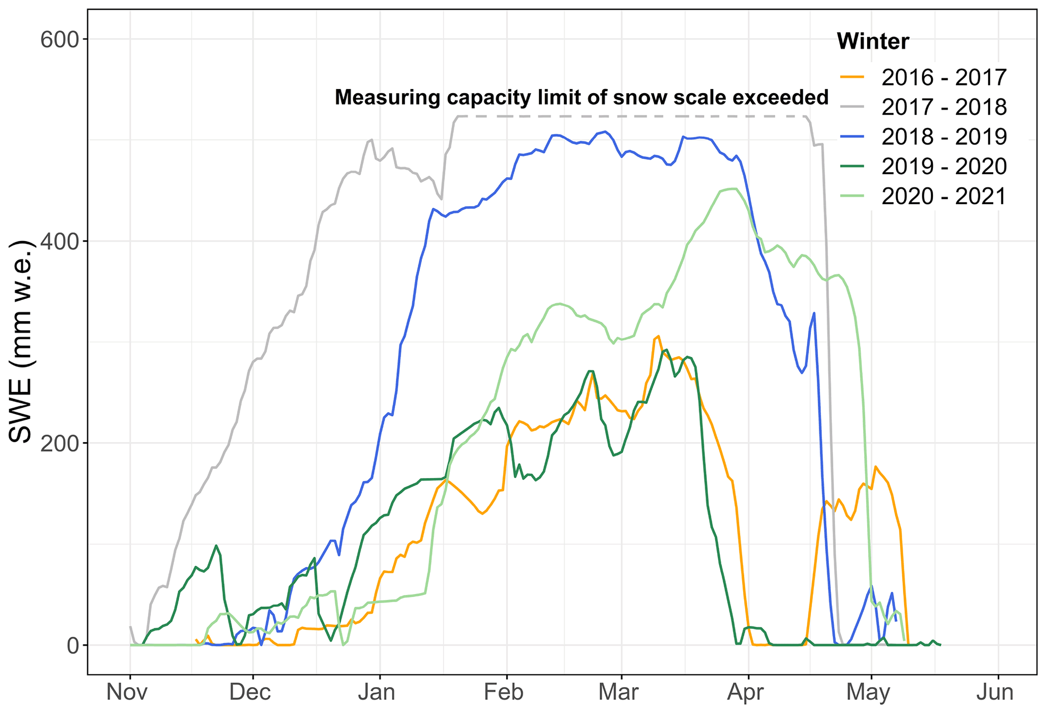
Figure 3Observed SWE (mm) at the Brunnenkopfhütte snow station (period: winter 2016/2017–2020/2021).
2.2 Datasets
The present study utilises three different datasets. Data sources and the aim of using these datasets are described below.
-
We use observed hydro-meteorological datasets from a test site (i.e. Brunnenkopfhütte) with the aim to show how the DDF of snow can be estimated for a specific site under naturally varying hydro-meteorological conditions.
-
In order to demonstrate the variation of the DDF over time, location, and altitude, as well as its significance for temperature-index modelling, we use elevation-zone temperature data of the upper Jhelum basin from a previous study (Bogacki and Ismail, 2016).
-
In the discussion section (Sect. 5), we perform a brief analysis in order to show the influence of climate change on the DDF in poorly monitored regions. In this specific analysis, projected changes in temperature are based on a previous study (Ismail et al., 2020). These projected changes in temperature are the median of four global climate models (GFDL-ESM2M, HadGEM2-ES, IPSL-CM5A-LR, and MIROC5) that are driven by two representative concentration pathways (RCP2.6 and RCP8.5). These data are provided by the Inter-Sectoral Impact Model Intercomparison Project (ISIMIP) (Hempel et al., 2013; Frieler et al., 2017).
The primary objective of this paper is to analyse the contribution of individual energy balance components to snowmelt, in order to better understand and predict how the lumped degree-day factor will vary with the season, latitude, altitude, and the actual meteorological conditions. In addition, we want to demonstrate following the approach of Walter et al. (2005) how these energy balance components can be estimated with minimal data requirements, as limited data availability is the major reason to apply temperature-index models.
3.1 Degree-day factor
The basic formulation of the degree-day method calculates daily snowmelt depth M (mm) by multiplying the number of degree days TDD (∘C d) with the degree-day factor DDF (mm ∘C−1 d−1) (Zingg, 1951; Braithwaite, 1995; Rango and Martinec, 1995).
Degree days TDD are only defined if a characteristic air temperature lies above a reference temperature T0; otherwise, TDD is set to 0 ∘C d. Typically, the freezing point T0 = 0 ∘C is chosen as reference temperature (DeWalle and Rango, 2008). Depending on the availability of temperature data, the characteristic air temperature is usually calculated as the mean of maximum and minimum daily air temperatures (Braithwaite, 1995) or the mean of hourly observations (Rango and Martinec, 1995; DeWalle and Rango, 2008). Other approaches like daily maximum temperature (Bagchi, 1983), integrating the positive part of a diurnal cycle (Ismail et al., 2015), or averaging the positive degree-day sum of m daily observations (Braithwaite and Hughes, 2022) are also common.
By a simple re-arrangement of Eq. (1) to
the DDF can be calculated for given degree days TDD, if the daily melt depth M is known either by observation or by calculation. Likewise, the portion of the degree-day factor DDFi associated with the melt depth Mi, which relates to any of the individual energy balance components (see Eq. 4), can be determined.
The energy needed to melt ice at 0 ∘C into liquid water at 0 ∘C is defined by the latent heat of fusion of ice (333.55 kJ kg−1). Thus the melt depth Mi caused by an energy flux Qi (W m−2) over a certain time period Δt (s) can be calculated from the relation (USACE, 1998; Hock, 2005)
where ρw is the density of water at 0 ∘C (999.84 kg m−3). In the context of degree-day factor models, the time period Δt is usually taken as 1 d = 86 400 s, though some authors (Hock, 1999; McGinn, 2012) have calculated degree-day factors also for sub-daily, e.g. hourly, periods. According to the relation given in Eq. (3), an energy flux of 1 W m−2 for a single day will result in a melt depth of 0.26 mm.
3.2 Energy balance
The energy flux available for snowmelt QM can be calculated from the balance of energy fluxes entering or leaving the snowpack and the change in the internal energy stored in the snowpack ΔQ (e.g. USACE, 1998):
where QS and QL are the net shortwave and longwave radiation, QH is the sensible heat, QE is the latent energy of condensation or vaporisation, QG is the heat conduction from the ground, and QP is the energy contained in precipitation (all terms in W m−2).
In the following sections, the individual components of the energy balance are discussed in more detail. As heat conduction from the ground into the snowpack is small and can be in general neglected except when first snow falls on warm ground (Anderson, 2006), the component QG is not considered in the further analysis.
3.2.1 Shortwave radiation
Shortwave radiation emitted from the Sun is usually the largest source of energy input to the snowpack. The net energy flux QS (W m−2) entering the snowpack by absorption of shortwave radiation is
where A is the snow albedo (–) and Si the incident solar radiation (W m−2) on the snow surface. A widely used approach (Masters, 2004; Yang and Koike, 2005; Badescu, 2008) to determine the incident solar radiation on Earth's surface is the introduction of a clearness index KT (–)
where S0 is the mean daily potential extraterrestrial solar radiation (W m−2) that would insolate a horizontal surface on the Earth's ground if no atmosphere would be present.
Potential insolation at the top of atmosphere
The potential insolation, which is only dependent on the changing position of the Sun during the year in relation to the geographic location of the incident point on the Earth's surface, can be calculated from the equation (Masters, 2004)
where GS is the solar constant (W m−2), dr the relative distance of the Earth to the Sun (–), ϕ the geographic latitude (rad) of the incident point, δ the solar declination (rad), and ωs the sunrise hour angle (rad). The solar constant GS is slightly varying with the occurrence of so-called sunspots. Measurements by Kopp and Lean (2011) indicate a present value of about 1361 W m−2.
Both Sun position variables, the relative distance of the Earth to the Sun and the solar declination, can be calculated quite exactly by rigorous astronomical algorithms (Meeus, 1991; Reda and Andreas, 2004), but for non-astronomical purposes, more simple formulas are sufficiently accurate. The relative distance of the Earth to the Sun, which varies throughout the year due to the elliptical orbit of the Earth, can be approximated by (Masters, 2004)
where J is the day number, with J = 1 on 1 January. The solar declination can be obtained from the sinusoidal relationship
which puts the spring equinox on day J = 81. Knowing the solar declination δ, the sunrise hour angle ωs can be calculated from
On the Northern Hemisphere, the maximum extraterrestrial radiation occurs at the summer solstice with a fairly identical mean daily energy flux of about 480 W m−2 over latitudes 30–60∘ N, as the Sun's lower-altitude angle at higher latitudes is compensated for by longer daylight hours. On the contrary, minimum extraterrestrial radiation at the winter solstice varies strongly with latitude, e.g. 227 W m−2 at 30∘ and only 24 W m−2 at 60∘ N.
Clearness index
When the solar radiation passes through the atmosphere, it is partly scattered and absorbed. While even on a clear day only about 75 % of the incoming radiation reaches the ground, by far the largest reflection is caused by clouds. A vast number of solar radiation models exist that parameterise this effect, which is denoted as clearness index KT or atmospheric transmissivity τ, as a function of meteorological variables. For a review see e.g. Evrendilek and Ertekin (2008), Ahmad and Tiwari (2011), or Ekici (2019).
A fundamental and widely used solar radiation model that is proposed in the context of evapotranspiration calculations (Allen et al., 1998) is the Ångström–Prescott model, which relates the clearness index to the relative sunshine duration
where n is the actual and N the maximal possible duration of sunshine (h), where the latter can be calculated from the sunrise hour angle ωs,
The parameters a and b in Eq. (11) are regression parameters that usually have to be fitted to observed global radiation. If no actual solar radiation data are available, the values a = 0.25 and b = 0.50 are recommended (Allen et al., 1998). Though the Ångström–Prescott model has the disadvantage that the parameters have to be fitted and the actual duration of sunshine has to be observed, it has the benefit that both parameters allow for a direct physical interpretation. The parameter a represents the clearness index KT on overcast days (n = 0), while their sum a+b gives the clearness index on clear days (n=N).
Commonly, in remote mountainous regions, only temperature data are available, due to which another group of solar radiation models is typically utilised. In these approaches the difference between daily maximum and minimum air temperature ΔT (∘C) is used as a proxy for cloud cover, as clear-sky conditions result in a higher temperature amplitude between day and night compared to overcast conditions. Typical models are the exponential approach proposed by Bristow and Campbell (1984) and its later modifications or the simple empirical equation by Hargreaves and Samani (1982).
with the empirical coefficient kH = 0.16 for inland and kH = 0.19 for coastal locations. Since the influence of cloud cover on the clearness index and thus on the DDF can be illustrated much more directly by Ångström–Prescott type models, this model type is used in the paper.
It is obvious that the attenuation of extraterrestrial solar radiation is a function of the distance the rays have to travel through the atmosphere, as absorption and scattering occurs all along the way. Several solar radiation models consider altitude as a variable, for which the models below were calibrated including high-altitude stations and are of Ångström–Prescott type; thus the altitude effects can be compared directly.
Jin et al. (2005):
Rensheng et al. (2006):
Liu et al. (2019):
For all models, z is the altitude (km) and ϕ the latitude (degree). In Eqs. (14) and (16) only the parameter a of Eq. (11) is a function of altitude z, while in Eqs. (15) and (17) also the parameter b is dependent on z.
In order to evaluate the altitude effect separately from other parameters, the clearness index KT is split into two components:
where is the clearness index at z = 0 m a.s.l. and Kz is a clearness altitude factor (–), which represents the increase in KT with altitude relative to . At sea level, Kz = 1 for all models and all values of relative sunshine duration . Though the clearness altitude factors Kz obtained from Eqs. (14)–(17) are different for each model, they all show a linear increase with altitude, the slope of which depends on the cloudiness (see Fig. 4). It should be noted that although Kz is higher for overcast than for clear-sky conditions, the absolute increase in the clearness index KT with altitude is higher under clear-sky conditions because of the higher base value . For example, at z = 2000 m a.s.l., the Jin (b) (Eq. 15) model has a clearness altitude factor Kz of 1.27 for overcast and 1.10 for clear-sky conditions. However, when multiplying by the respective clearness factors at sea level of 0.15 and 0.72, the resulting clearness indices KT at z= 2000 m a.s.l. increase by 0.04 under overcast and 0.07 under clear-sky conditions to an absolute value of 0.19 and 0.79, respectively.
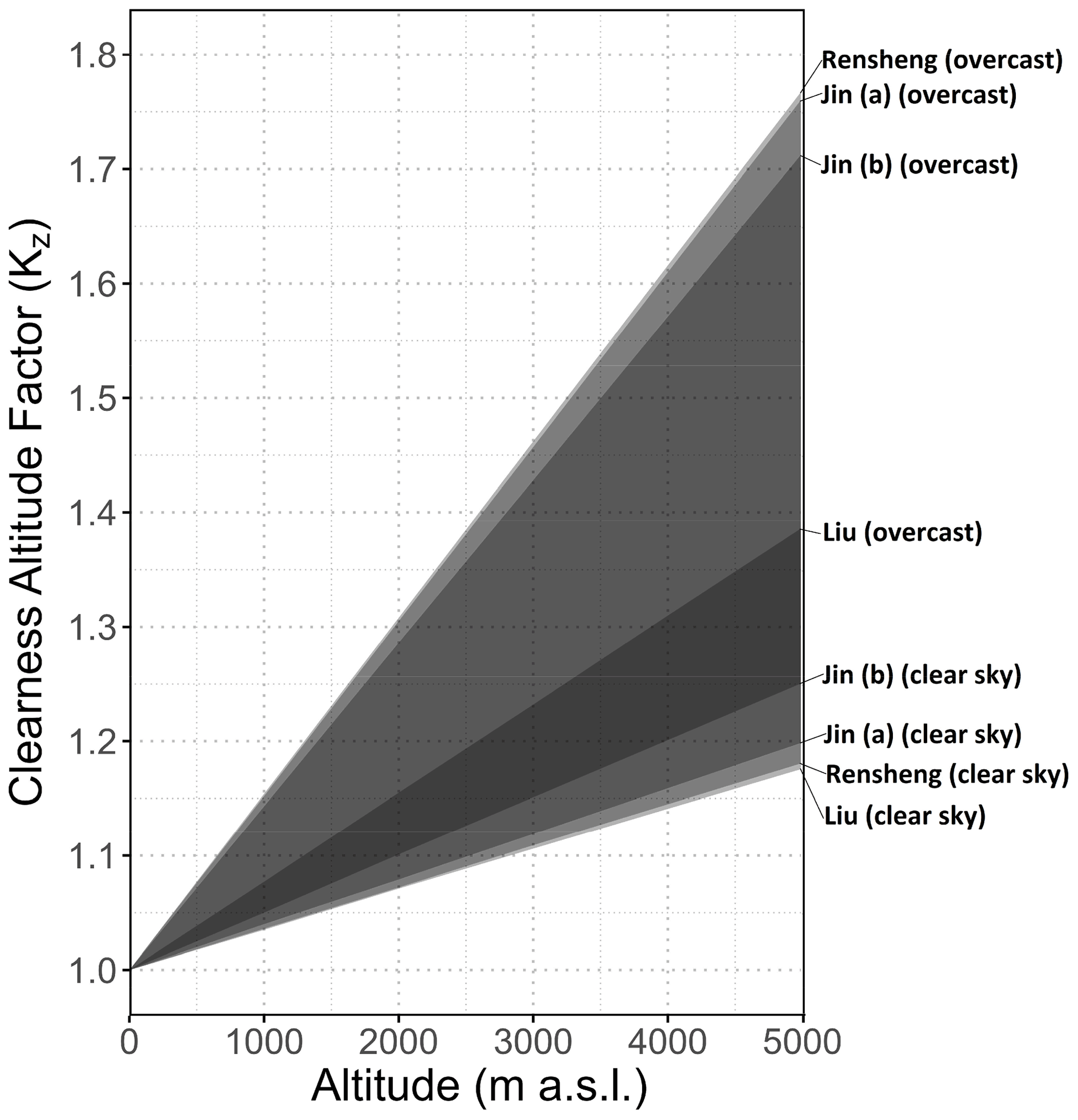
Figure 4Clearness altitude factor Kz for latitude 45∘ and different altitudes, based on different models presented in Eqs. (14)–(17) (i.e. Jin (a), Jin (b), Rensheng, and Liu).
Albedo
While the albedo of fresh snow is well above 0.9 (Hock, 2005), indicating that most of the shortwave radiation is reflected, it may drop significantly within a few days due to snow metamorphism. Well-aged snow generally has an albedo in the range of 0.4–0.5 (Anderson, 2006). Snow albedo is primarily dependent on the grain size of the snow crystals near the surface but also on aerosols in the snow and dust deposits. Respective snow albedo models are proposed by Wiscombe and Warren (1980), Warren and Wiscombe (1980), or Amaral et al. (2017). However, because of their data requirements, surrogate exponential decay models as formulated by USACE (1956) are commonly in use, which assumes the decrease in albedo as a function of time after the last significant snowfall. For example, Walter et al. (2005) use the empirical relationship
where An−1 is the albedo of the previous day and Amax is the maximum albedo (∼ 0.95) of fresh snow. Following Eq. (19), the snow albedo will decrease from 0.95 to 0.52 after 10 d and to 0.43 after 30 d if no new snowfall occurs.
3.2.2 Longwave radiation
The net longwave radiation flux over the snow surface QL (W m−2) is the balance between incoming longwave radiation that is emitted by the atmosphere QL,in (W m−2) and outgoing radiation from the snowpack QL,out (W m−2).
Longwave radiation is a function of the temperature of the emitting body and can be calculated with the Stefan–Boltzmann law:
where L is the radiative flux (W m−2), ε and T are the emissivity (–) and the absolute temperature (K) of the emitting body, respectively, and σ is the Stefan-Boltzmann constant ( W m−2 K−4).
In particular, fresh snow is nearly a perfect blackbody with respect to longwave radiation with a high emissivity of 0.99 (Warren, 1982; USACE, 1998; Anderson, 2006). For old snow, Brutsaert (1982) gives an emissivity value of 0.97. Given a melting snowpack having a surface temperature of 0 ∘C, the outgoing energy flux can be taken as constant with W m−2.
For the atmospheric longwave radiation, usually the air temperature Ta (K) is used in Eq. (21). However, while the snowpack longwave emissivity is virtually constant, the emissivity of the atmosphere is highly variable. Typical values under clear-sky conditions range from 0.6–0.8, primarily depending on air temperature and humidity (Anderson, 2006), whereas for overcast conditions it can be close to 1.0.
A number of empirical and more physically based approaches exist to estimate atmospheric longwave emissivity from standard meteorological data (see Hock, 2005, for a discussion). For clear-sky conditions, Brutsaert (1975) developed a theoretically based formula depending on air temperature and vapour pressure measured at screen level:
where εac is the clear-sky longwave emissivity (–), pv the actual vapour pressure (hPa), and Ta the air temperature (K). Later, Brutsaert reconciled Eq. (22) with an empirical approach proposed by Swinbank (1963),
that considers the strong correlation between vapour pressure and air temperature; thus, only air temperature is needed as input variable. Using the above relation, at an air temperature of 10 ∘C the atmospheric longwave radiation flux into the snowpack amounts to QL,in = 281 W m−2 under clear-sky conditions, which is less than the outgoing flux of 310 W m−2; i.e. the snowpack will lose energy in this situation.
The variability of atmospheric emissivity due to cloud cover, which increases the longwave emissivity, is significantly higher than variations under clear-sky conditions. Monteith and Unsworth (2013) give the simple linear relationship
where εa is the atmospheric longwave emissivity, c is the fraction of cloud cover (–), and εac is calculated by Eqs. (22) or (23). For overcast conditions and an air temperature of 10 ∘C, Eq. (24) yields an atmospheric emissivity of 0.96, which results in an atmospheric longwave radiation flux of QL,in = 351 W m−2 and thus a positive flux of QL = 41 W m−2 into the snowpack.
Although cloud cover is difficult to parameterise, as clouds can be highly variable in space and time and their effects on radiation depend on the different cloud genera, a strong correlation between cloud cover and sunshine duration is obvious. Doorenbos and Pruitt (1977) give a tabulated relation between cloudiness c and relative sunshine hours (see Eq. 11), which can be fitted by the quadratic regression
Nevertheless, in simple sky models usually a linear relation between cloudiness and relative sunshine hours is applied as a first approximation (e.g. Brutsaert, 1982; Annandale et al., 2002; Pelkowski, 2009), which, as Badescu and Paulescu (2011) showed by using probability distributions to develop relations between cloudiness and relative sunshine hours, is a first good estimate.
3.2.3 Sensible heat exchange
Sensible heat exchange describes the energy flux due to temperature differences between the air and the snow surface while air is permanently exchanged by wind turbulence. A frequent approach to parameterise turbulent heat transfer is the aerodynamic method, which explicitly includes wind speed as a variable (Braithwaite et al., 1998; Lehning et al., 2002; Hock, 2005):
where ρa is the air density (kg m−3), cp the specific (isobaric) heat capacity of air (1006 J kg−1 ∘C−1), CH the exchange coefficient for sensible heat (–), u the mean wind speed (m s−1), Ta the air temperature (∘C), and Ts the temperature at the snow surface (∘C).
The density of air ρa is a function of atmospheric pressure, air temperature, and humidity:
where p is the atmospheric pressure (Pa), pv the vapour pressure (Pa) (see Eq. 32), Ta the air temperature (K), Md the molar mass of dry air (0.02897 kg mol−1), R the universal gas constant (8.31446 J mol−1 K−1), and e the ratio of molar weights of water and dry air equal to 0.622. At usual air temperatures humidity has only a minor effect on the air density.
The decrease in atmospheric pressure with altitude z (m a.s.l.) can be estimated by the isothermal barometric formula
where p0 is the atmospheric pressure at sea level (Pa) and g the gravitational acceleration (m s−2). At an air temperature of 0 ∘C and a standard atmospheric pressure at sea level of 101.325 kPa, the air density is 1.29 kg m−3, while for example at an altitude of 2000 m a.s.l. the atmospheric pressure reduces to 78.9 kPa and the air density becomes 1.01 kg m−3.
The exchange coefficient CH can be approximated with (Campbell and Norman, 1998)
where k is the von Kármán constant 0.41 (–), zu and zT the height of wind and temperature observation above the snow surface (m), zm the momentum roughness parameter, and zh the heat roughness parameter. For a snow surface, the roughness parameters are given by Walter et al. (2005) as zm∼0.001 m and zh∼0.0002 m.
As it can be seen from Eq. (26), the sensible heat component depends mainly on wind speed and temperature. During stable clear weather periods with typically light winds, the turbulent exchange is smaller on average than the radiation components. For example, a wind speed of 1 m s−1 and an air temperature of 5 ∘C will result in a sensible heat flux of about 15.5 W m−2. However, at warm rain events or at föhn conditions with strong warm winds, turbulent exchange can significantly contribute to the melting process. For example, a föhn event of 14 h duration on 8 December 2006 at Altdorf (Switzerland, 440 m a.s.l.) with an average air temperature of about 16 ∘C, average relative humidity of 37 %, and average wind speed of 14.6 m s−1 resulted in a mean sensible heat flux of about 700 W m−2 during that duration.
3.2.4 Latent energy of condensation or vaporisation
The latent energy exchange reflects the phase change of water vapour at the snow surface, either by condensation of vapour contained in the air or by vaporisation of snow. Thus, it can either warm or cool the snowpack (Harpold and Brooks, 2018). The energy flux is dependent on the vapour gradient between the air and the snow surface and is, like the sensible heat exchange, a turbulent process that increases with the wind speed. Thus, the aerodynamic formulation is analogous to Eq. (26):
where λv is the latent heat of vaporisation of water at 0 ∘C (2.501×10⁶ J kg−1); CE the exchange coefficient for latent heat (–), which is assumed to be equal to the exchange coefficient for sensible heat CH; qa the specific humidity of the air (–); and qs the specific humidity at the snow surface (–).
The specific humidity qa can be derived from measurements of relative humidity or dew point temperature. In cases where such data are not available, Walter et al. (2005) approximate the dew point temperature by the minimum daily temperature. For any air temperature T (∘C), the saturation vapour pressure ps (Pa) can be calculated by an empirical expression known as the Magnus–Tetens equation in the general form (Lawrence, 2005)
where A, B, and C are coefficients after Allen et al. (1998): A = 17.2694, B = 237.3 ∘C, and C = 610.78 Pa. At the snow surface, according to Lehning et al. (2002) the air temperature can be assumed equal to the snow surface temperature, and Eq. (31) is applied with coefficients for saturation vapour pressure over ice: A = 21.8746, B = 265.5 ∘C, C = 610.78 Pa (Murray, 1967). At a temperature of 0 ∘C, both coefficient sets yield the same saturation vapour pressure of ps = 611 Pa.
Knowing the relative humidity ψ (–) and the saturation vapour pressure ps at a given air temperature, the actual vapour pressure pv (Pa) can be calculated through the relation
and subsequently the respective specific humidity by
with p the atmospheric pressure (Pa) and e the ratio of molar weights of water and dry air equal to 0.622 as in Eq. (27). Assuming melting conditions with a snow temperature Ts = 0 ∘C and saturated vapour conditions, the vapour pressure at the snow surface is (0 ∘C) = 611 Pa. While at positive air temperatures the sensible heat flux is always warming the snowpack, the latent heat flux can cool the snow by vaporisation if the relative humidity of the air is low. Even when assuming a relative humidity of 100 %, the latent heat flux into the snowpack will be comparatively small if wind speed is low, e.g. about 13 W m−2 at an air temperature of 5 ∘C and a wind speed of 1 m s−1.
3.2.5 Precipitation heat
The heat transfer into the snowpack by lowering the rain's temperature, which is usually assumed to be equal to the air temperature Ta (∘C), down to the freezing point at 0 ∘C can be estimated as
where cw is the specific heat capacity of water (4.2 kJ kg−1 ∘C−1) and P is the daily rainfall depth (kg m−2 d−1). The energy input from precipitation is usually quite small, and even during extreme weather conditions, like heavy warm rain storms with temperatures of 15 ∘C and a precipitation depth of 50 mm, that may occur, e.g. during early winter in the Alps, the mean daily energy flux from rain would be a moderate 36.5 W m−2.
3.2.6 Change in internal energy
The rate of change in the energy stored in the snowpack ΔQ (W m−2) represents the internal energy gains and losses due to changes in the snowpack's temperature profile and due to phase changes, i.e. melting of the ice portion or refreezing of liquid water in the snowpack. Until the snowpack temperature is isothermal at 0 ∘C, any melt produced in the surface layer that exceeds the liquid water holding capacity of the porous snow matrix will percolate downward and will be captured and refrozen in colder lower layers. This internal mass and energy transport process absorbs at least parts of the incoming energy, which reduces the energy available for melt and will thus reduce the actual DDF.
Under data-scarce conditions and particularly when only daily data are available, it is difficult to properly quantify the change in the internal energy of the snowpack (see discussion in Sect. 5.2.1). Therefore, in our study we focus on melt periods when the snowpack is “ripe”, i.e. when the snowpack temperature is isothermal at 0 ∘C and the residual volumetric water content of about 8 % (Lehning et al., 2002) is filled with liquid water. This assumption is not a limitation when analysing the contribution of each individual energy flux component towards a resulting DDF as presented in following sections, but the additional energy needed for warming the snowpack has to be taken into account when estimating the total DDF if a snowpack is not ripe (see Fig. 11).
In this section, the contribution of each energy flux component Qi to the lumped daily DDF is presented. For this purpose, the respective melt depth Mi is calculated according to Eq. (3) and further converted into the corresponding degree-day factor component DDFi using Eq. (2). For the following exemplary calculations, the air temperature is assumed to stay always above 0 ∘C; thus, degree days TDD (∘C d) in Eq. (2) have the same numerical value as the daily average air temperature Ta (∘C) used in the calculation of several energy flux components.
Besides demonstrating the dependency of the DDF components on decisive parameters of the energy flux components, the presented tables in the Supplement (“S” in numbering of figures and tables means that they are in the Supplement) and graphs in this section, which are based on the relationships given in Sect. 3, can be used to estimate the DDF component values if observed data are either not available or not sufficient for more sophisticated approaches. It should be noted that parameters are normalised where applicable, i.e. set to hypothetical values like clearness index KT = 1 or wind speed u = 1.0 m s−1; thus, final DDF values can be obtained by multiplying the given figures by the actual values of those parameters. Furthermore, all results are based on the assumption that the snowpack is isothermal at 0 ∘C and in a fully ripe state.
4.1 Shortwave radiation component – DDFS
Shortwave-radiation-induced melt is usually considered the largest DDF component, especially at higher elevations as well as under dry climates. The net energy flux QS is calculated using Eq. (5), which consists of three factors: (a) latitude, (b) albedo, and (c) clearness index KT. The dependency of DDFS on these factors is demonstrated in Fig. 5 for the period between winter solstice (21 December) and summer solstice (21 June). As shortwave radiation is independent of air temperature and hence of degree days, the corresponding melt is divided by a hypothetical degree-day value of 1 ∘C d to arrive at the presented DDFS values. In the event of actually higher degree days, the given DDFS values have to be divided accordingly.
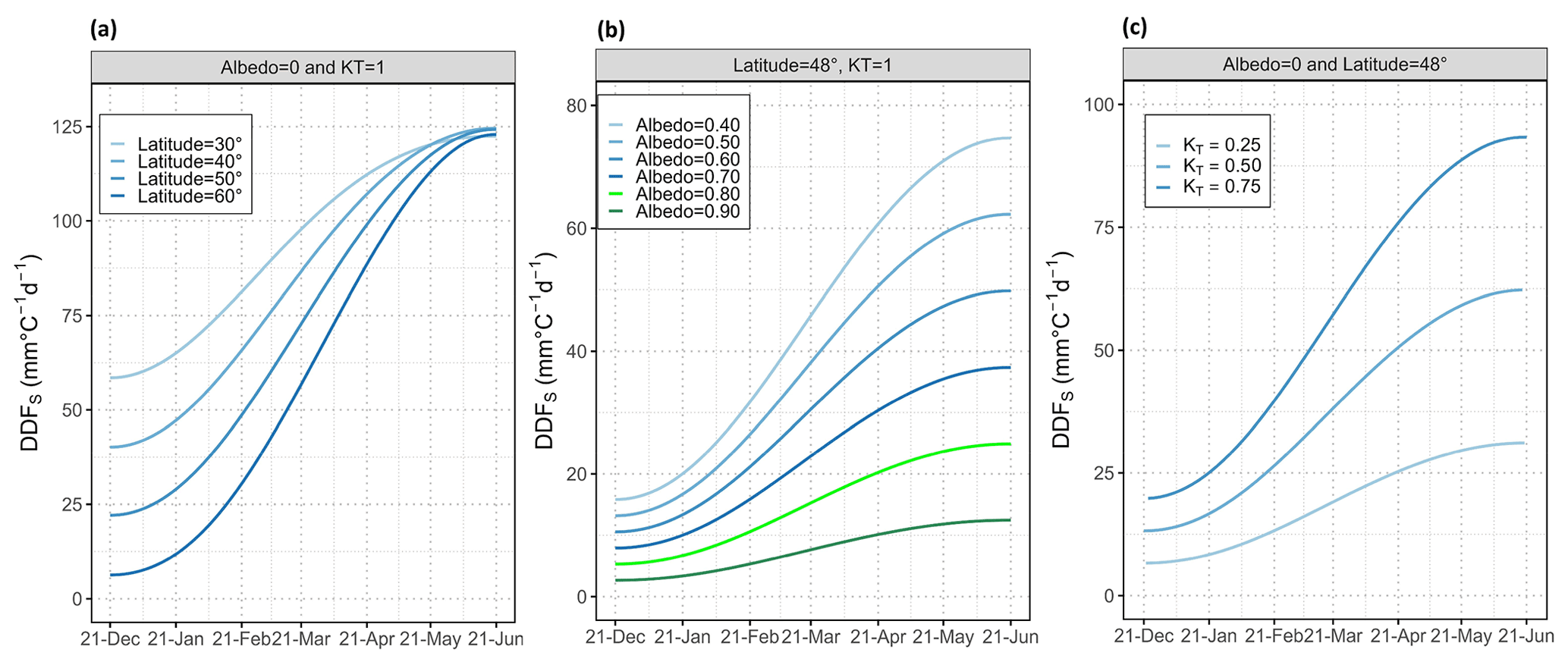
Figure 5Variation of solar-radiation-based DDFS for a degree-day value of 1 ∘C d for (a) different latitudes under constant snow albedo and clearness index, (b) snow albedos under constant latitude and clearness index, and (c) different clearness indices under constant latitude and snow albedo. The latitude = 48∘ corresponds to the location of the Brunnenkopfhütte test site.
Figure 5a shows the variation of DDFS depending on latitude for the range 30–60∘ N, while albedo (A = 0) and clearness index (KT = 1) are set constant. Obviously, there is a significant difference in DDFS for different latitudes around the winter solstice due to solar inclination, making latitude the predominant factor for DDFS at this time of the year. However, around the summer solstice, DDFS has nearly the same value at different latitudes because the lower solar angle at higher latitudes is counterweighted by a larger hour angle, i.e. longer sunlight hours. Thus, with the progress of the melting season, the factors albedo and clearness index become more important than latitude.
Figure 5b shows the influence of albedo on the DDFS at a given latitude (Brunnenkopfhütte test site – latitude 48∘) and normalised constant clearness index (KT = 1). Snow albedo varies between 0.9–0.4, covering the range between fresh and well-aged snow. As expected, the influence of albedo increases with increasing incoming solar radiation towards the summer solstice. A good estimate of albedo is therefore much more important when the snowmelt season progresses than in early spring. If for example the same degree-day value of 10 ∘C d is assumed on 21 March and on 21 May, the difference in DDFS between fresh (A = 0.9) and aged (A = 0.4) snow would be 0.8 and 4.6 mm ∘C−1 d−1 in March compared to 1.2 and 7.1 mm ∘C−1 d−1 in May, respectively.
The dependency of DDFS on the clearness index KT is shown in Fig. 5c. In line with Eq. (6), DDFS values under clear sky (KT = 0.75) are always higher than under overcast conditions (KT = 0.25). Similar to albedo, the influence of the clearness index becomes more pronounced, with increasing solar angle when the snowmelt season progresses.
The influence of altitude on DDFS in terms of increasing KT values can be assessed by multiplying a clearness index at sea level, which may be obtained by any of the numerous solar radiation models, with a clearness altitude factor Kz (see Eq. 18). Figure 4 shows the range of clearness altitude factors for latitude 45∘ derived from Eqs. (14)–(17). All Kz values show a linear increase with altitude, with the slope depending on cloudiness. It should be noted that although the increase in Kz relative to is higher under overcast than under clear-sky conditions, the absolute increase in the clearness index KT with altitude is larger for clear-sky conditions (see Sect. 3.2.1). When using the intersection of all models and sky conditions, which is indicated by the dark grey area in Fig. 4, in order to get one overall rough estimate of Kz for all conditions, the clearness altitude factor and thus the resulting DDFS are found to increase by about 6.4 % per each 1000 m of altitude.
4.2 Longwave radiation component – DDFL
The net longwave energy flux QL is calculated using Eq. (21), in which the outgoing radiation from the snowpack can be assumed to be constant. Thus, the contribution of the longwave radiation component DDFL is mainly dependent on the air temperature and the emissivity of the atmosphere (e.g. in particularly cloudiness conditions). Figure 6 and Table S1 present the DDFL as a function of degree days TDD and cloudiness. For a wide range of degree days, especially in conjunction with low cloudiness, the outgoing longwave energy flux is higher than the incoming, resulting in a theoretically negative degree-day factor that will reduce the total DDF. This means that the DDFL component under clear-sky conditions is usually contributing to a cooling of the snowpack rather than to melting. Under overcast conditions, the DDFL is relatively constant around 1 mm ∘C−1 d−1 with a maximum value of 1.3 mm ∘C−1 d−1 at TDD = 20 ∘C d. Although this contribution to the total DDF is small compared to the shortwave radiation component DDFS, it can be of importance at the onset of snowmelt in early spring, when the solar radiation is still low and the albedo of fresh snow is high.
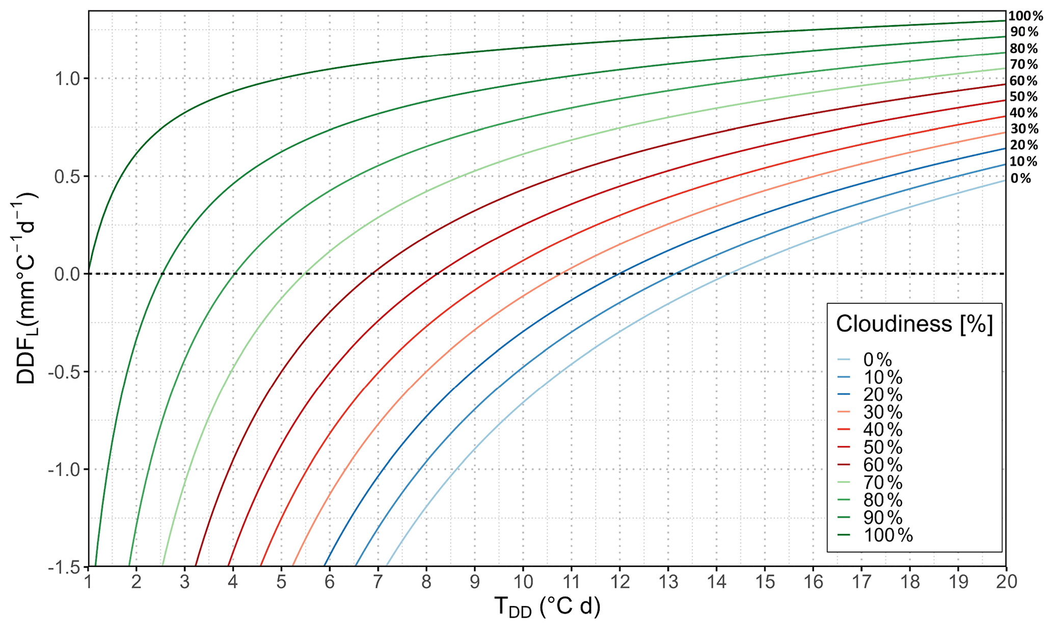
Figure 6Longwave radiation component (DDFL) for selected cloudiness (%) and degree days (∘C d).
4.3 Sensible heat component – DDFH
The sensible heat flux QH as given by Eq. (26) is mainly proportional to wind speed and the temperature difference between the air and the snow surface. Furthermore, air density, besides its dependency on temperature, is a function of relative humidity and atmospheric pressure, and thus of altitude (Eqs. 27 and 28). Since the influence of the relative humidity on air density is negligible, a relative humidity of RH = 0 % is assumed in the below analysis on the response of the DDFH to changes in temperature and degree days, wind speed, and altitude. It should be noted that this analysis assumes typical melt conditions with a snowpack temperature of Ts = 0 ∘C and positive air temperature, whereas negative air temperature would lead to a negative sensible heat flux resulting in a cooling of the snowpack and a decrease in total DDF.
Figure 7 and Table S2 show the variation in DDFH depending on altitude and degree days, while the wind speed is assumed to be constant at u=1 m s−1. The latter allows the DDFH to be easily calculated for any other wind speed by multiplying the given value by the actual wind speed. The DDFH principally decreases with altitude, with less pronounced differences due to temperature at higher altitudes. However, the most important factor is the wind speed. For example, with a daily average wind speed of u = 1.0 m s−1, e.g. at sea level z = 0 m a.s.l., the DDFH only decreases from 0.806 to 0.781 mm ∘C−1 d−1 when degree days increase from 1 to 10 ∘C d (see Fig. 7 and Table S2). In contrast, for a degree day of 1 ∘C d, the DDFH increases proportionally from 0.806 to 8.061 mm ∘C−1 d−1 when wind speed increases from 1 to 10 m s−1. Thus, wind speed is a decisive variable when estimating the DDFH.
If wind speed observations are not available, they may be roughly estimated based on the topographic and climate characteristics of the study area. However, average values may not represent the actual wind conditions and thus DDFH on a certain day. While for example the geometric mean of observed daily wind speed at the Brunnenkopfhütte station is about 0.8 m s−1, resulting in a DDFH of approx. 0.7 mm ∘C−1 d−1, the maximum daily average wind speed is about 4.5 m s−1, which increases DDFH to approx. 3.9 mm ∘C−1 d−1.

Figure 7Variation of sensible heat component (DDFH) at different altitude based on different degree days, RH = 0 %, and u = 1 m s−1.
4.4 Latent heat component – DDFE
The latent heat flux QE approximated by an aerodynamic model as in Eq. (30) indicates that the latent heat component DDFE is mainly dependent on the humidity gradient near the snow surface and on the wind speed. Additionally, altitude has an influence, as the air density decreases with altitude. Figure 8 and Table S3 give the resulting DDFE as a function of degree days for different values of relative humidity and at daily average wind of u = 1.0 m s−1, whereas air density values are assumed at an elevation of 0 m a.s.l. In line with the sensible heat component DDFH, DDFE for any other wind speed can be obtained by multiplication by the actual value. For relative humidity < 30 % the DDFE is negative over the whole range of degree days; hence, the latent heat component will reduce the total DDF under these conditions. Even if the air is humid and warm, contribution of latent heat is moderate, e.g. DDFE=1.0 mm ∘C−1 d−1 at a relative humidity of 100 % and TDD = 20 ∘C d.
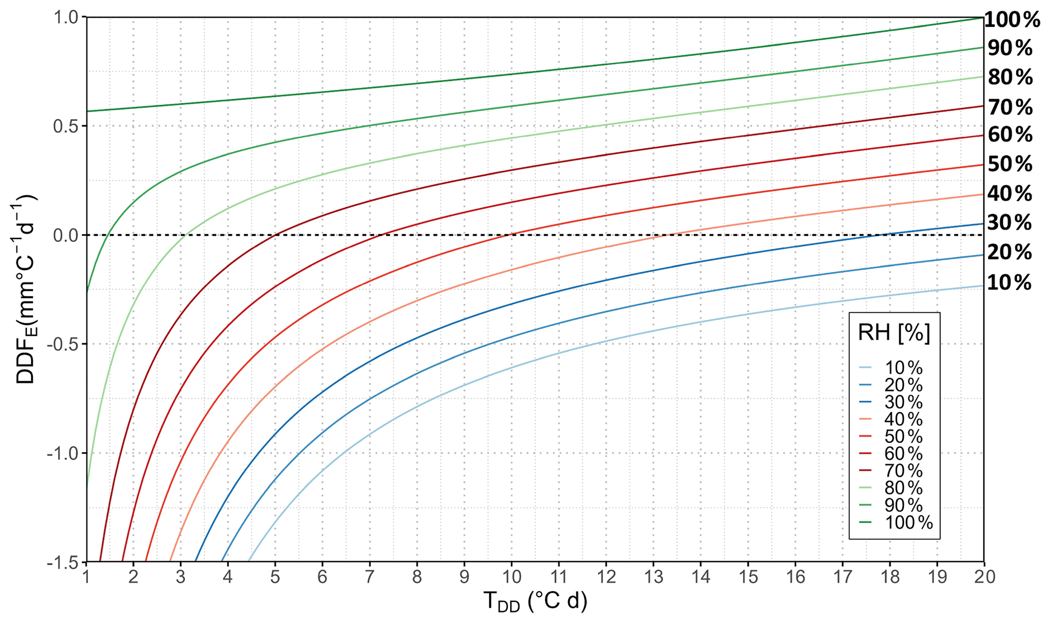
Figure 8Latent heat component (DDFE) for selected relative humidity (%), degree days (∘C d), and u = 1 (m s−1), These values are for u=1 m s−1; for a different wind speed these values can be multiplied for the desired wind speed. Air density values are assumed at an elevation of 0 m a.s.l.
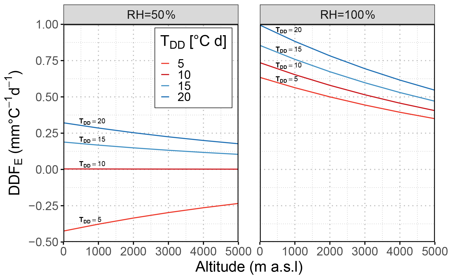
Figure 9Variation of latent heat component (DDFE) depending on altitude for different relative humidity values, degree days, and u = 1 m s−1.
Figure 9 shows the combined effect of altitude, relative humidity, and temperature on DDFE. At a high relative humidity (e.g. RH = 100 %), similar to the DDFH the DDFE values principally decrease with altitude, with less pronounced differences due to temperature at higher altitudes. At lower relative humidity (e.g. RH = 50 %), the altitude effect is less noticeable, and at low temperatures even a reversal of the effect can be observed. Thus, altitude reduces the positive DDFE associated with high humidity, while it also reduces the cooling effect of a negative latent heat flux, which is associated with low humidity and lower air temperature.
As the above analysis shows, humidity is the main variable influencing the DDFE. In general, humid air will promote condensation at a cooler snow surface, which releases latent energy and contributes to a positive DDF, while dry air will promote evaporation and sublimation from the snow surface, which abstracts energy from the snowpack. Thus, mainly depending on the humidity of the air, the latent heat energy flux is usually a heat sink, while only in the event of high humidity in conjunction with higher temperature it becomes a heat source to the snowpack. Especially in spring, when relative humidity is comparatively low in middle and northern latitudes, large parts of the incoming solar radiation can be consumed by evaporation from the snow surface, significantly reducing the energy available for melt and thus reducing the corresponding DDFs (Lang and Braun, 1990; Zhang et al., 2006).
4.5 Precipitation heat component – DDFP
Rainfall can affect the snowpack energy budget by adding sensible heat due to warm rain and by releasing latent heat if the rain refreezes in the snowpack (DeWalle and Rango, 2008). The latter effect is not considered in this study, as the snowpack is assumed at a 0 ∘C melting condition. Given that the precipitation heat QP is linearly dependent on air temperature in Eq. (34), a division by respective degree days makes DDFP independent of temperature and proportional to rainfall, resulting in a DDFP = 0.0125 mm ∘C−1 d−1 for a precipitation depth of 1 mm d−1. DDFP for any other precipitation can be obtained by respective multiplication. The exemplary values in Table 2 show, however, that the contribution of the precipitation heat component DDFP is modest compared to other DDF components. Even high rainfall of 50 mm d−1 would release only a small amount of sensible heat, resulting in a DDFP of 0.6 mm ∘C−1 d−1.
Table 2Precipitation heat component (DDFP) (mm ∘C−1 d−1) for selected precipitation (mm d−1).

While the previous section focuses on the characteristics of each individual energy-flux-based DDF component, this section mainly discusses the influence of spatial, seasonal, or meteorological conditions on the overall DDF. The discussion section bifurcates into two sub-sections: (i) influence of individual factors on the DDF, such as latitude, altitude, albedo, season, and rain on snow events, and (ii) application of energy-flux-based DDF estimates, discussing how this value can be estimated for a temperature-index model by using different available datasets and applied under varying meteorological and climate change conditions.
5.1 Influence of individual factors on the DDF
In this section all conclusions are under the assumption that the snowpack is isothermal at Ts=0 ∘C and in ripe condition; hence, all net incoming energy is available for melt and contributes to the total DDF. Apart from the discussed variables, we assumed the standard values of u = 1 m s−1, RH = 70 %, A=0.5, and P = 0 mm and typical melt conditions of TDD = 5 ∘C d, unless otherwise stated.
5.1.1 Influence of latitude
While topographic factors like slope, aspect, or shading in mountainous regions result in a high local variability of melt conditions, larger-scale regional patterns of DDFs (e.g. a dependency on latitude) could not be detected in a data review by Hock (2003). This observation is supported by a brief analysis of the effect of latitude below, where the DDF is compared not on the same date but on the same degree days. As an illustrative example, typical melt conditions of TDD = 5 ∘C d at a latitude of about 35∘ N in the upper Jhelum catchment (Bogacki and Ismail, 2016) are compared to similar conditions at a latitude of 48∘ N (Brunnenkopfhütte, 1602 m a.s.l.). As zone-wise temperature data (see Sect. 2.2) indicate, in the upper Jhelum catchment at an elevation zone of 1500–2000 m a.s.l., melting conditions usually occur around mid-February, while at Brunnenkopfhütte comparable degree days are obtained about 1 month later in mid-March. Figure 10a compares the energy-flux-based DDF components at both latitudes. The decisive solar radiation component is very similar at the two locations, both under clear-sky and overcast conditions; thus the total DDF is virtually identical at both latitudes. Therefore, at least in moderate latitudes and when compared under similar melt conditions, no significant effect of latitude on DDF could be found.
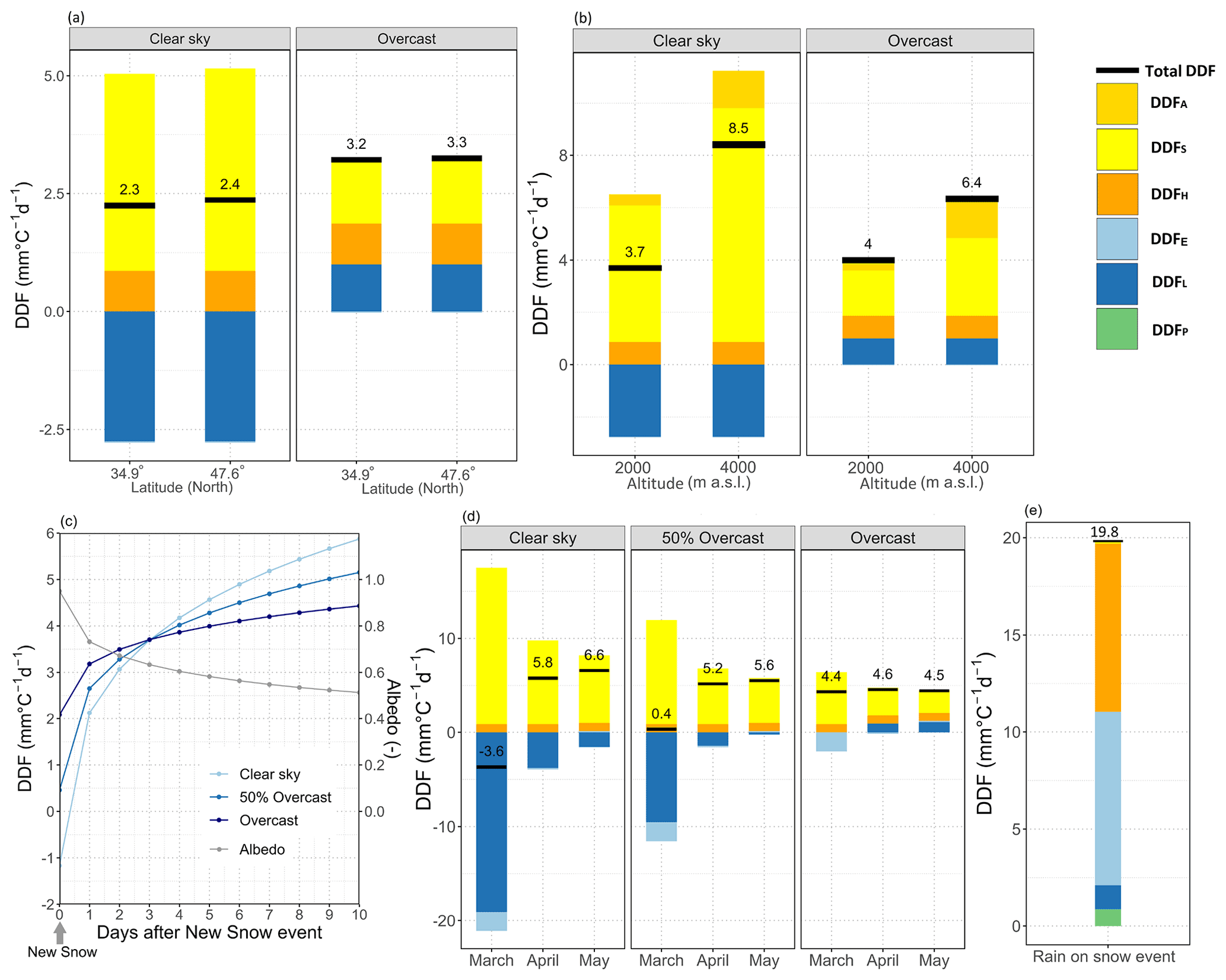
Figure 10Influence of (a) latitude, (b) altitude, (c) albedo, (d) season, and (e) rain on snow events on the DDF under clear-sky and overcast conditions. DDF components: shortwave radiation (DDFS), longwave radiation (DDFL), sensible heat (DDFH), latent heat (DDFE), precipitation heat (DDFP) and increase in shortwave component due to the increase in the clearness index with altitude (DDFA).
5.1.2 Influence of altitude
Contrary to the compensating effect in the case of latitude, the delayed onset of snowmelt due to altitude influences the DDF noticeably, which becomes important in temperature-index models where calculation is usually based on elevation bands. In order to demonstrate the influence of altitude on the DDF, two elevation zones with an altitude of 1500–2000 and 3500–4000 m a.s.l., respectively, are compared at 35∘ latitude in the upper Jhelum catchment. As indicated above, typical melt conditions of TDD = 5 ∘C d occur at 1500–2000 m a.s.l. usually around mid-February, while at 3500–4000 m a.s.l. similar degree days are obtained for mid-May. The resulting DDFs (see Fig. 10b) show a significant difference, both under clear-sky conditions and under overcast conditions, because of the different input in solar radiation caused by the alteration in solar angle between February and May. Figure 10b shows an additional term DDFA on top of the solar radiation component that represents the increase in incoming solar radiation due to the clearness altitude factor, which takes into account the increase in the clearness index with altitude (see Sect. 3.2.1). Averaging the factors proposed by different solar radiation models (see Fig. 4) results in an additional component DDFA of 0.4 and 1.4 mm ∘C−1 d−1 under clear-sky conditions and of 0.5 and 1.6 mm ∘C−1 d−1 under overcast conditions at 1500–2000 and 3500–4000 m a.s.l., respectively.
While snow albedo is assumed constant at 0.5 in Fig. 10b, taking into consideration the decrease in albedo as the snow ages (see Table 1, e.g. A=0.74 in February and A=0.42 in May) results in a more pronounced difference with altitude, i.e. a DDF of 0.3 compared to 10.5 mm ∘C−1 d−1 under clear-sky conditions and of 2.7 versus 7.3 mm ∘C−1 d−1 under overcast conditions for the two altitudes, respectively.
The increase in DDF with increasing altitude is in line with previous studies (e.g. Hock, 2003; Kayastha and Kayastha, 2020). For example, in the Nepalese Himalayan region, seasonal-average DDF increases from 7.7 to 11.6 mm d−1 ∘C−1 with respect to altitude ranging 4900 to 5300 m a.s.l. (Kayastha et al., 2000), whereas Kayastha and Kayastha (2020) found that the model-calibrated range of the DDF in the central Himalayan basin varies between 7.0–9.0 mm d−1 ∘C−1 over an approximate altitude range of 4000–8000 m a.s.l. As Kayastha et al. (2000) pointed out, higher values of the DDF usually occur at very low temperatures since at higher altitudes the major driving factor for melt is the energy input by solar radiation.
5.1.3 Influence of albedo
As already discussed in the sections before, snow albedo is a critical parameter for the DDF since according to Eq. (5) the albedo directly controls the net solar radiation flux into the snowpack. While albedo of fresh snow is well above 0.9, hence reflecting most of the incoming shortwave radiation, it drops rapidly when larger grains form due to snow metamorphism. Figure 10c demonstrates the effect of ageing snow after a new snow event, when a simple exponential decay model as given in Eq. (19) is used and typical melting conditions TDD = 5 ∘C d are assumed. Since directly after a new snow event (Day = 0) the fresh snow albedo is high (A=0.95), the overall DDF is generally small. Under clear-sky conditions, if longwave radiation cooling is larger than net shortwave radiation flux, even a negative DDF value, i.e. no melt, may occur. If there is no new snow event in between, albedo will decrease following the exponential decay model to 0.52 after 10 d, resulting in a DDF of 5.8 mm ∘C−1 d−1 under clear-sky conditions and 4.4 mm ∘C−1 d−1 under overcast conditions. The increase in the DDF with exponential decay in albedo is in agreement with the findings of MacDougall et al. (2011), who found that the DDF is sensitive to albedo with values of > 4.0 mm d−1 ∘C−1 at an albedo of 0.6. As described qualitatively in the literature (e.g. Hock, 2003), under all sky conditions the DDF continuously increases with decreasing albedo, with the increase, however, being more pronounced under clear-sky than under overcast conditions.
5.1.4 Influence of season
Since the solar angle rises from its minimum at the winter solstice in December to its maximum on 21 June, the solar radiation component DDFS increases during the snowmelt season, and thus the DDF is expected to increase. Figure 10d shows the influence of season on the DDF at the Brunnenkopfhütte test site during the melt period, assuming average degree days of 1, 4, and 7 ∘C d in March, April, and May, respectively (see Table 1). Under clear-sky conditions, the total DDF increases from a negative value of −3.6 mm ∘C−1 d−1 in March to 6.6 mm ∘C−1 d−1 in May. Under overcast conditions, however, the DDF is virtually stable, ranging from 4.4 to 4.5 mm ∘C−1 d−1 in the same period. The stability of the DDF under overcast conditions found in our study is in agreement with the study of Kayastha et al. (2000), where the DDFs observed during July–August are small compared to June because of prevailing cloud cover due to monsoon activity, which reduces the incoming shortwave radiation.
An evaluation of the individual DDF components shows that under clear-sky conditions the high impact of solar radiation in combination with low degree days at the onset of the snowmelt season is counterweighted by a strong negative longwave radiation component that decreases as the season progresses. Under overcast conditions, DDFL is neutral or slightly positive, while the DDFS component decreases because degree days rise faster than the input from solar radiation, which implies that sky conditions (i.e. overcast, and clear sky) are more decisive for an estimate of the DDF than the day of the year.
The effect of cloud cover is further amplified by the decrease in albedo while the melt season progresses, which becomes more significant under clear-sky conditions. In the present example (with the average monthly albedo as specified in Table 1) only 30 % of incoming solar radiation is contributing to melt in March, while it is about 60 % in May, enhancing the marked increase in the DDF under clear-sky conditions.
5.1.5 Influence of rain on snow events
In general, the precipitation heat component alone has only a minor effect on the DDF. However, in conjunction with certain weather conditions, like breaking in of warm and moist air, rain over snow events may lead to sudden melt and severe flooding.
Figure 10e shows the different DDF components resulting from a hypothetical rain over snow events assuming an air temperature of 15 ∘C, a precipitation of 70 mm d−1, a daily average wind speed of 10 m s−1, a relative humidity of 100 %, and overcast conditions. Although the amount of precipitation is substantial and the rain temperature is comparatively high, the contribution of DDFP is still modest. However, air temperature, relative humidity, and in particular wind speed associated with such events increase the sensible and latent heat components significantly. Thus, the resulting overall DDF is much higher than under usual melt conditions, which may lead to a considerable melt that adds to the runoff already caused by the heavy rain.
5.2 Application of energy-flux-based DDF estimates
5.2.1 DDF estimates under field conditions
In addition to the analysis of the influence of individual factors on the DDF, the dataset from the Brunnenkopfhütte test site is used to compare energy-flux-based estimates with field-derived DDFs in order to demonstrate how naturally varying meteorological conditions during the melt season, and in particular the cold content of the snowpack, affect the accuracy of DDF estimates.
For this purpose, daily melt was estimated from the daily difference of observed snow water equivalent during melt periods (see Fig. 3). Energy-flux-based melt was calculated by the formulas given in Sect. 3 using observed daily data from the Brunnenkopfhütte automatic snow and weather station (e.g. air temperature, wind speed; see Sect. 2.1) where applicable.
The daily degree-day sum is calculated from hourly air temperature data as proposed by Braithwaite and Hughes (2022). In general, operational degree-day models typically use constant degree-day factors for a certain time period (e.g. 10 d period). In this backdrop, both energy-flux-based and data-derived daily melt values were accumulated on a 10 d basis and divided by the degree days of the respective period. The 10 d averaging procedure also smooths daily noise in the observed data, in particular inaccuracies in the determination of daily melt and unrealistic DDF values because of daily temperature averages just above 0 ∘C.
The comparison between field-derived and estimated (energy-flux-based) DDFs (see Fig. 11) yields a fair agreement with bias = 0.14 mm ∘C−1 d−1 between estimated and field-derived values, and root mean square error (RMSE) = 1.12 mm ∘C−1 d−1. Noteworthy in Fig. 11 are the new snow events, where the snowpack is no longer ripe and a certain amount of the incoming energy is needed to bring the snowpack back to ripe state, thus does not contributing to melt. For these events all estimated DDFs considerably overestimate the field-derived ones and were thus excluded from the calculation of the error metrics.
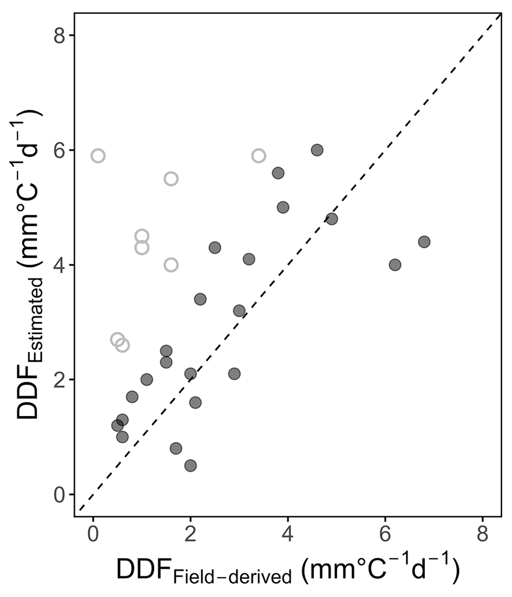
Figure 11Comparison of field-derived vs. estimated (energy-flux-based) 10 d DDF for the Brunnenkopfhütte test site (period: November 2016–May 2021) – hollow points represent DDFs during periods with new snow events (new snow: precipitation ≥ 5 mm d−1).
It is of interest to estimate DDFs also in cases where the snowpack is not ripe, e.g. because of new snow events or due to radiational cooling during clear cold nights. An approach to account for the snowpack's energy deficit, i.e. the energy needed to bring the snowpack temperature isothermal at 0 ∘C, is the concept of cold content (Marks et al., 1999; Schaefli and Huss, 2011). The cold content is usually either estimated as a function of meteorological parameters or calculated by keeping track of the residuals of the snowpack energy balance (Jennings et al., 2018). For the latter, the SNOWPACK model (Lehning et al., 2002) is an excellent tool, which provides a highly detailed simulation of the vertical mass, energy, and besides other state variables the snow temperature distribution inside a snowpack. However, SNOWPACK requires a considerable number of meteorological input variables and preferably at least hourly observations, both of which are usually not available in the context where degree-day models are employed.
Especially suited for data-scarce conditions, Walter et al. (2005) apply a lumped approach that accounts for the cold content by changing the (isothermal) snowpack temperature depending on the daily net energy flux. When the incoming energy flux is sufficient to raise the snow temperature to 0 ∘C or when it is already at 0 ∘C the day before, all additional available energy produces melt. This approach, which does not need any additional data, however, seems to significantly overestimate the snowpack temperature particularly in situations with negative energy fluxes at night but a positive daily net balance, as a comparison with SNOWPACK simulations using data from Brunnenkopfhütte shows (see Sect. S2 in the Supplement). Therefore, an appropriate parameterisation of the cold content under limited data availability that would enable satisfactory estimates of DDFs in situations when the snowpack is not completely ripe remains subject to further research.
5.2.2 DDF estimates for temperature-index modelling
Snowmelt runoff models using the temperature-index approach have proven to be useful tools for simulation and forecasting in large snow- or glacier-dominated catchments, particularly in remote mountainous regions where data are usually scarce. A good estimate of the degree-day factor as the decisive model parameter is important either to stay in a realistic range when calibrating this parameter or in the case of forecasting when estimating its changes while the season progresses. In order to demonstrate the alteration of DDFs over time and altitude, energy-flux-based DDFs are estimated using 10 d average temperature (i.e. period 2000–2015) for the key elevation zones in the upper Jhelum catchment (Bogacki and Ismail, 2016). In the current example, the upper Jhelum catchment is discussed because of elevation-zone-wise data availability in comparison to test site where only point data are available (for more details, see Sect. 2). Because of the lack of data other than temperature and precipitation, prevailing conditions during the melt season are crudely approximated by the standard conditions used in this section, assuming persistent clear-sky conditions and albedo declining according to Eq. (19) after the last fresh snow event just before the beginning of the melting period.
Figure 12 shows the overall picture of how the DDF for snow will change over time and under climate change (i.e. present, RCP2.6, and RCP8.5; for DDF estimates under climate change, see Sect. 5.2.3). For example, Fig. 12a shows the development of DDFs in the elevation zones over time. As expected, melt starts earlier in lower-elevation zones and successively progresses to higher altitudes. Interestingly, the DDF in the first 10 d period of melting in each elevation zone increases with altitude. This is a combined effect of (i) higher solar radiation input and decreasing albedo while the season progresses and (ii) the onset of melt in higher-elevation zones starting at a lower degree-day threshold than in lower zones. In contrast to Fig. 10d, the DDF in Fig. 12 decreases continuously in all elevation zones in the subsequent melting periods since air temperature and thus degree days rise faster than melt. The range of DDFs for snow estimated by the energy flux components is in good agreement with earlier studies for the Himalayan region, e.g. 7.7–11.6 mm d−1 ∘C−1 (Kayastha et al., 2000), 5–9 mm d−1 ∘C−1 (Zhang et al., 2006), 5–7 mm d−1 ∘C−1 (Tahir et al., 2011), and 7.0–9.0 mm d−1 ∘C−1 (Kayastha and Kayastha, 2020).

Figure 12(a) DDF estimates for a temperature-index modelling in the present climate; (b) influence of climate change – 2071–2100 under RCP2.6; (c) influence of climate change – 2071–2100 under RCP8.5.
5.2.3 DDF estimates under the influence of climate change
Climate change will ultimately influence snowmelt patterns depending on the projected changes in temperature and precipitation. In recent studies, usually model parameters including DDFs are considered as constant when assessing the climate change impact on future water availability from snow and glacier fed catchments (Lutz et al., 2016; Hasson et al., 2019; Ismail et al., 2020). However, due to the physical processes on which they depend, these parameters are subject to climate change. In this section, an attempt is made to estimate the influence of climate change on the DDFs in different elevation zones. For this analysis, results from ISIMIP data (see Sect. 2.2), which predict the temperature change for the period 2071–2100 to ΔT = 2.3 ∘C under RCP2.6 and ΔT = 6.5 ∘C under RCP8.5, are added to the temperatures in the present climate for each elevation zone.
The first effect to be observed in Fig. 12b and c is the common finding that snowmelt will start earlier under climate change as temperatures rise earlier above freezing. In addition, due to being earlier in the year, the DDFs in corresponding elevation zones are generally smaller compared to the current climate, though there are some outliers at the start of melting, due to division by low degree-day values. In the case of the pessimistic RCP8.5 scenario (Fig. 12c), a seasonal snow cover will no longer be established in the lowest elevation zone (i.e. 2500–3000 m a.s.l.) as air temperature at this elevation is projected to stay well above freezing throughout the winter. In general, the results of this brief analysis indicate that the DDFs are expected to decrease under the influence of climate change, as the snowmelt season will shift earlier in the year when solar radiation is small and snow albedo values are expected to be on the higher side. Musselman et al. (2017) highlight similar findings about slower snowmelt in a warmer world due to a shift of the snowmelt season to a time of lower available energy. These results may contribute the important aspect to the recent discussion on the linearity of temperature-index models used for glacier mass balance predictions (Bolibar et al., 2022; Vincent and Thibert, 2022) that the key impact of climate change on the DDF is the shift in the melt season. This effect should be larger on snowmelt because the entire melt season will be shifted to a time with lower solar radiation, while the period of glacial melt in the present climate will be preserved and will only start earlier and last longer under climate change.
Degree-day models are common and valuable tools for assessing present and future water availability in large snow- or glacier-melt-dominated basins, in particular when data are scarce like in the Hindu Kush–Karakoram–Himalayas mountain ranges. The present study attempts to quantify the effects of spatial, temporal, and climatic conditions on the degree-day factor (DDF), in order to gain a better understanding of which influencing factors are decisive under which conditions. While this analysis is physically based on the energy balance, formulas with minimum data requirement for estimating the DDFs are used to account for situations where observed data are limited. In addition, resulting tables (see Sect. S1 in the Supplement) and graphs for typical melt conditions are provided for a quick assessment. A comparison between field-derived and estimated DDFs at the Brunnenkopfhütte test site shows a fair agreement with bias = 0.14 mm ∘C−1 d−1 and RMSE = 1.12 mm ∘C−1 d−1 over periods without new snow events, since fresh snow increases the cold content of the snowpack and contradicts the condition of the snowpack being ripe and isothermal at 0 ∘C. Further research is needed for cases where, under the constraint of limited data availability, also changes in the cold content of the snowpack are to be considered, with a specific focus on approaches that parameterise the diurnal dynamics of vertical temperature distribution in the snowpack.
Furthermore, the use of these DDF estimates directly as a model parameter or the incorporation of an energy-balance-based DDF approach into a degree-day model is not intended. One important aspect of temperature-index models is that the DDF is a lumped parameter, which is usually subject to calibration and accounts for uncertainties in different variables and parameters, i.e. temperature estimates, runoff coefficients, etc. Thus, the DDFs estimated by the energy balance approach are rather aimed to validate the results of parameter calibration and to highlight necessary adjustments due to climate change.
The analysis of the energy-balance processes controlling snowmelt indicates that cloud cover is the most decisive factor for the dynamics of the DDF. Under overcast conditions, the contribution of shortwave radiation is comparatively low, whereas the other components are in general small. Therefore, the total DDF value is not very high, and variations due to other factors are usually limited, apart from exceptional rainstorm events, for which energy balance models are the more suitable approach.
Under clear-sky conditions, on the other hand, shortwave radiation is the most prominent component contributing to melt. The increase in solar angle while the melt season progresses in combination with declining albedo and a decreasing cooling effect by the longwave radiation component along with increasing air temperature leads to a pronounced temporal dynamic in the DDF. Whereas incoming solar radiation and net longwave radiation can be determined fairly accurate by under clear-sky conditions, albedo becomes the crucial parameter for estimating the DDF, especially when new snow events occur during the melt period.
Clear-sky conditions promote the effect of increasing DDF with altitude if similar melting conditions are compared, since melting temperatures arrive later in the season at higher altitudes. The opposite effect can be observed with regard to climate change. Under higher temperatures at a given altitude, climate change will shift the snowmelt season earlier in the year. Consequently, when comparing periods of similar degree days, our study suggests DDFs are to decrease, since solar radiation is to generally decrease and albedo to typically increase.
Therefore, and as pointed out by many researchers, the DDF cannot be considered as a constant model parameter. Rather, its spatial and temporal variability must be taken into account, especially when using temperature-index models for forecasting present or predicting future snowpack and glacier changes, as well as the resulting water availability projections.
Snow and meteorological station datasets used in this study can be acquired upon request from Lothar Kirschbauer (kirschbauer@hs-koblenz.de) of the Koblenz University of Applied Sciences.
The supplement related to this article is available online at: https://doi.org/10.5194/tc-17-211-2023-supplement.
MFI and WB conceived the study, performed the analysis, and wrote the paper. MD supervised the study as well as provided input in the review and editing process. MS and LK took part in several field campaigns acquiring in situ data and helped in the review process. All authors participated in the discussion of the results.
The contact author has declared that none of the authors has any competing interests.
Publisher's note: Copernicus Publications remains neutral with regard to jurisdictional claims in published maps and institutional affiliations.
We also thank Koblenz University of Applied Sciences for providing the snow and meteorological station data. We would like to thank all the reviewers and editor and in particular Roger Braithwaite for their valuable comments which helped to improve the manuscript considerably.
This work was supported by the German Research Foundation (DFG) and the Technical University of Munich (TUM) in the framework of the Open Access Publishing Program.
This paper was edited by Harry Zekollari and reviewed by Roger Braithwaite, Rijan Kayastha, Álvaro Ayala, and Lander Van Tricht.
Ahmad, M. J. and Tiwari, G. N.: Solar radiation models-A review, Int. J. Energy Res., 35, 271–290, https://doi.org/10.1002/er.1690, 2011.
Allen, R. G., Pereira, L. S., Raes, D., and Smith, M.: Crop evapotranspiration – guidelines for computing crop water requirements, FAO Irrigation and Drainage Paper 56, FAO, Rome, Italy, 300 pp., 1998.
Amaral, T., Wake, C. P., Dibb, J. E., Burakowski, E. A., and Stampone, M.: A simple model of snow albedo decay using observations from the Community Collaborative Rain, Hail, and Snow-Albedo (CoCoRaHS-Albedo) Network, J. Glaciol., 63, 877–887, https://doi.org/10.1017/jog.2017.54, 2017.
Ambach, W.: Characteristics of the Heat Balance of the Greenland Ice sheet for Modelling, J. Glaciol., 31, 3–12, https://doi.org/10.3189/S0022143000004925, 1985.
Anderson, E. A.: National Weather Service river forecast system-snow accumulation and ablation model. National Oceanographic and Atmospheric Administration (NOAA), Tech. Mem., NWS HYDRO-17, US Dept. of Commerce, Silver Spring, MD, 217 pp., https://repository.library.noaa.gov/view/noaa/13507 (last access: 3 January 2023), 1973.
Anderson, E. A.: Snow Accumulation and Ablation Model – SNOW-17, NOAA's National Weather Service, Office of Hydrologic Development, Silver Spring, https://www.weather.gov/media/owp/oh/hrl/docs/22snow17.pdf (last access: 3 January 2023), 2006.
Annandale, J., Jovanovic, N., Benadé, N., and Allen, R.: Software for missing data error analysis of Penman-Monteith reference evapotranspiration, Irrigation Sci., 21, 57–67, https://doi.org/10.1007/s002710100047, 2002.
Arendt, A. A. and Sharp, M. J.: Energy balance measurements on a Canadian high Arctic glacier and their implications for mass balance modelling, IAHS-AISH publication, 256, 165–172, 1999.
Asaoka, Y. and Kominami, Y.: Incorporation of satellite-derived snow-cover area in spatial snowmelt modeling for a large area: determination of a gridded degree-day factor, Ann. Glaciol., 54, 205–213, https://doi.org/10.3189/2013AoG62A218, 2013.
Badescu, V. (Ed.): Modeling solar radiation at the earth's surface: recent advances, Springer, Berlin, 517 pp., https://doi.org/10.1007/978-3-540-77455-6, 2008.
Badescu, V. and Paulescu, M.: Statistical properties of the sunshine number illustrated with measurements from Timisoara (Romania), Atmos. Res., 101, 194–204, https://doi.org/10.1016/j.atmosres.2011.02.009, 2011.
Bagchi, A. K.: Areal value of degree-day factor/Valeur spatiale du facteur degré-jour, Hydrolog. Sci. J., 28, 499–511, https://doi.org/10.1080/02626668309491991, 1983.
Bergström, S.: Development and application conceptual runoff model for scandinavian catchments, SMHI, Research Department, Hydrology, 162 pp., http://urn.kb.se/resolve?urn=urn:nbn:se:smhi:diva-5738 (last access: 3 January 2023), 1976.
Bogacki, W. and Ismail, M. F.: Seasonal forecast of Kharif flows from Upper Jhelum catchment, Proc. IAHS, 374, 137–142, https://doi.org/10.5194/piahs-374-137-2016, 2016.
Bolibar, J., Rabatel, A., Gouttevin, I., Zekollari, H., and Galiez, C.: Nonlinear sensitivity of glacier mass balance to future climate change unveiled by deep learning, Nat. Commun., 13, 409, https://doi.org/10.1038/s41467-022-28033-0, 2022.
Bormann, K. J., Evans, J. P., and McCabe, M. F.: Constraining snowmelt in a temperature-index model using simulated snow densities, J. Hydrol., 517, 652–667, https://doi.org/10.1016/j.jhydrol.2014.05.073, 2014.
Braithwaite, R. J.: Positive degree-day factors for ablation on the Greenland ice sheet studied by energy-balance modelling, J. Glaciol., 41, 153–160, https://doi.org/10.3189/S0022143000017846, 1995.
Braithwaite, R. J.: Temperature and precipitation climate at the equilibrium-line altitude of glaciers expressed by the degree-day factor for melting snow, J. Glaciol., 54, 437–444, https://doi.org/10.3189/002214308785836968, 2008.
Braithwaite, R. J. and Hughes, P. D.: Positive degree-day sums in the Alps: a direct link between glacier melt and international climate policy, J. Glaciol., 68, 901–911, https://doi.org/10.1017/jog.2021.140, 2022.
Braithwaite, R. J., Konzelmann, T., Marty, C., and Olesen, O. B.: Reconnaissance Study of glacier energy balance in North Greenland, 1993–94, J. Glaciol., 44, 239–247, https://doi.org/10.3189/S0022143000002586, 1998.
Braun, L., Grabs, W., and Rana, B.: Application of a Conceptual Precipitation Runoff Model in the Langtang Kfaola Basin, Nepal Himalaya, Snow and Glacier Hydrology, 1993.
Braun, L. N.: Simulation of snowmelt-runoff in lowland and lower alpine regions of Switzerland, PhD Thesis, ETH Zurich, https://doi.org/10.3929/ETHZ-A-000334295, 1984.
Bristow, K. L. and Campbell, G. S.: On the relationship between incoming solar radiation and daily maximum and minimum temperature, Agri. Forest Meteorol., 31, 159–166, https://doi.org/10.1016/0168-1923(84)90017-0, 1984.
Brutsaert, W.: On a derivable formula for long-wave radiation from clear skies, Water Resour. Res., 11, 742–744, https://doi.org/10.1029/WR011i005p00742, 1975.
Brutsaert, W.: Evaporation into the Atmosphere, Springer Netherlands, Dordrecht, https://doi.org/10.1007/978-94-017-1497-6, 1982.
Campbell, G. S. and Norman, J. M.: Introduction to environmental biophysics, 2nd Edn., Springer, New York, 286 pp., https://www.umfcv.ro/files/!/x/4/_/4_ Intro_Env_MED_.pdf (last access: 3 January 2023), 1998.
Carenzo, M., Pellicciotti, F., Rimkus, S., and Burlando, P.: Assessing the transferability and robustness of an enhanced temperature-index glacier-melt model, J. Glaciol., 55, 258–274, https://doi.org/10.3189/002214309788608804, 2009.
DeWalle, D. R. and Rango, A.: Principles of Snow Hydrology, Cambridge University Press, Cambridge, https://doi.org/10.1017/CBO9780511535673, 2008.
Doorenbos, J. and Pruitt, W. O.: Guidelines for predicting crop water requirements, Rev., Food and Agriculture Organization of the United Nations, Rome, 144 pp., https://www.posmet.ufv.br/wp-content/uploads/2015/08/LIVRO-385-Doorenbos-e-Pruitt-Guidelines-for-predicting-crop-water-requirements.pdf (last access: 3 January 2023) 1977.
Ekici, C.: Total Global Solar Radiation Estimation Models and Applications: A review, International Journal of Innovative Technology and Interdisciplinary Sciences, 2, 212–228, https://doi.org/10.15157/IJITIS.2019.2.2.212-228, 2019.
Evrendilek, F. and Ertekin, C.: Assessing solar radiation models using multiple variables over Turkey, Clim. Dynam., 31, 131–149, https://doi.org/10.1007/s00382-007-0338-6, 2008.
Frieler, K., Lange, S., Piontek, F., Reyer, C. P. O., Schewe, J., Warszawski, L., Zhao, F., Chini, L., Denvil, S., Emanuel, K., Geiger, T., Halladay, K., Hurtt, G., Mengel, M., Murakami, D., Ostberg, S., Popp, A., Riva, R., Stevanovic, M., Suzuki, T., Volkholz, J., Burke, E., Ciais, P., Ebi, K., Eddy, T. D., Elliott, J., Galbraith, E., Gosling, S. N., Hattermann, F., Hickler, T., Hinkel, J., Hof, C., Huber, V., Jägermeyr, J., Krysanova, V., Marcé, R., Müller Schmied, H., Mouratiadou, I., Pierson, D., Tittensor, D. P., Vautard, R., van Vliet, M., Biber, M. F., Betts, R. A., Bodirsky, B. L., Deryng, D., Frolking, S., Jones, C. D., Lotze, H. K., Lotze-Campen, H., Sahajpal, R., Thonicke, K., Tian, H., and Yamagata, Y.: Assessing the impacts of 1.5 °C global warming – simulation protocol of the Inter-Sectoral Impact Model Intercomparison Project (ISIMIP2b), Geosci. Model Dev., 10, 4321–4345, https://doi.org/10.5194/gmd-10-4321-2017, 2017.
Gafurov, A.: Water balance modeling using remote sensing information: focus on Central Asia, PhD Thesis, Inst. für Wasserbau, Stuttgart, 116 pp., 2010.
Hargreaves, G. H. and Samani, Z. A.: Estimating Potential Evapotranspiration, J. Irrig. Drain. Div., 108, 225–230, https://doi.org/10.1061/JRCEA4.0001390, 1982.
Harpold, A. A. and Brooks, P. D.: Humidity determines snowpack ablation under a warming climate, P. Natl. Acad. Sci. USA, 115, 1215–1220, https://doi.org/10.1073/pnas.1716789115, 2018.
Hasson, S., Saeed, F., Böhner, J., and Schleussner, C.-F.: Water availability in Pakistan from Hindukush–Karakoram–Himalayan watersheds at 1.5 ∘C and 2 ∘C Paris Agreement targets, Adv. Water Resour., 131, 103365, https://doi.org/10.1016/j.advwatres.2019.06.010, 2019.
He, Z. H., Parajka, J., Tian, F. Q., and Blöschl, G.: Estimating degree-day factors from MODIS for snowmelt runoff modeling, Hydrol. Earth Syst. Sci., 18, 4773–4789, https://doi.org/10.5194/hess-18-4773-2014, 2014.
Hempel, S., Frieler, K., Warszawski, L., Schewe, J., and Piontek, F.: A trend-preserving bias correction – the ISI-MIP approach, Earth Syst. Dynam., 4, 219–236, https://doi.org/10.5194/esd-4-219-2013, 2013.
Hinzman, L. D. and Kane, D. L.: Snow hydrology of a headwater Arctic basin: 2. Conceptual analysis and computer modeling, Water Resour. Res., 27, 1111–1121, https://doi.org/10.1029/91WR00261, 1991.
Hock, R.: A distributed temperature-index ice- and snowmelt model including potential direct solar radiation, J. Glaciol., 45, 101–111, https://doi.org/10.3189/S0022143000003087, 1999.
Hock, R.: Temperature index melt modelling in mountain areas, J. Hydrol., 282, 104–115, https://doi.org/10.1016/S0022-1694(03)00257-9, 2003.
Hock, R.: Glacier melt: a review of processes and their modelling, Prog. Phys. Geog., 29, 362–391, https://doi.org/10.1191/0309133305pp453ra, 2005.
Hock, R. and Noetzli, C.: Areal melt and discharge modelling of Storglaciären, Sweden, Ann. Glaciol., 24, 211–216, https://doi.org/10.3189/S0260305500012192, 1997.
Huss, M. and Hock, R.: Global-scale hydrological response to future glacier mass loss, Nat. Clim. Change, 8, 135–140, https://doi.org/10.1038/s41558-017-0049-x, 2018.
Immerzeel, W. W., Droogers, P., de Jong, S. M., and Bierkens, M. F. P.: Large-scale monitoring of snow cover and runoff simulation in Himalayan river basins using remote sensing, Remote Sens. Environ., 113, 40–49, https://doi.org/10.1016/j.rse.2008.08.010, 2009.
Immerzeel, W. W., Lutz, A. F., Andrade, M., Bahl, A., Biemans, H., Bolch, T., Hyde, S., Brumby, S., Davies, B. J., Elmore, A. C., Emmer, A., Feng, M., Fernández, A., Haritashya, U., Kargel, J. S., Koppes, M., Kraaijenbrink, P. D. A., Kulkarni, A. V., Mayewski, P. A., Nepal, S., Pacheco, P., Painter, T. H., Pellicciotti, F., Rajaram, H., Rupper, S., Sinisalo, A., Shrestha, A. B., Viviroli, D., Wada, Y., Xiao, C., Yao, T., and Baillie, J. E. M.: Importance and vulnerability of the world's water towers, Nature, 577, 364–369, https://doi.org/10.1038/s41586-019-1822-y, 2020.
Ismail, M. F. and Bogacki, W.: Scenario approach for the seasonal forecast of Kharif flows from the Upper Indus Basin, Hydrol. Earth Syst. Sci., 22, 1391–1409, https://doi.org/10.5194/hess-22-1391-2018, 2018.
Ismail, M. F., Bogacki, W., and Muhammad, N.: Degree-day factor models for forecasting the snowmelt runoff for Naran watershed, Sci. Int., 27, 1951–1960, 2015.
Ismail, M. F., Naz, B. S., Wortmann, M., Disse, M., Bowling, L. C., and Bogacki, W.: Comparison of two model calibration approaches and their influence on future projections under climate change in the Upper Indus Basin, Climatic Change, 163, 1227–1246, https://doi.org/10.1007/s10584-020-02902-3, 2020.
Jansson, P., Hock, R., and Schneider, T.: The concept of glacier storage: a review, J. Hydrol., 282, 116–129, https://doi.org/10.1016/S0022-1694(03)00258-0, 2003.
Jennings, K. S., Kittel, T. G. F., and Molotch, N. P.: Observations and simulations of the seasonal evolution of snowpack cold content and its relation to snowmelt and the snowpack energy budget, The Cryosphere, 12, 1595–1614, https://doi.org/10.5194/tc-12-1595-2018, 2018.
Jin, Z., Yezheng, W., and Gang, Y.: General formula for estimation of monthly average daily global solar radiation in China, Energ. Convers. Managem., 46, 257–268, https://doi.org/10.1016/j.enconman.2004.02.020, 2005.
Kane, D. L., Gieck, R. E., and Hinzman, L. D.: Snowmelt Modeling at Small Alaskan Arctic Watershed, J. Hydrol. Eng., 2, 204–210, https://doi.org/10.1061/(ASCE)1084-0699(1997)2:4(204), 1997.
Kayastha, R. B. and Kayastha, R.: Glacio-Hydrological Degree-Day Model (GDM) Useful for the Himalayan River Basins, in: Himalayan Weather and Climate and their Impact on the Environment, edited by: Dimri, A. P., Bookhagen, B., Stoffel, M., and Yasunari, T., Springer International Publishing, Cham, 379–398, https://doi.org/10.1007/978-3-030-29684-1_19, 2020.
Kayastha, R. B., Ageta, Y., and Nakawo, M.: Positive degree-day factors for ablation on glaciers in the Nepalese Himalayas: case study on Glacier AX010 in Shorong Himal, Nepal, Bulletin of Glaciological Research, 17, 1–10, 2000.
Kayastha, R. B., Yutaka, A., Masayoshi, N., Koji, F., Akiko, S., and Yoshihiro, M.: Positive degree-day factors for ice ablation on four glaciers in the Nepalese Himalayas and Qinghai-Tibetan Plateau, Bulletin of Glaciological Research, 20, 7–14, 2003.
Klok, E. J., Jasper, K., Roelofsma, K. P., Gurtz, J., and Badoux, A.: Distributed hydrological modelling of a heavily glaciated Alpine river basin, Hydrolog. Sci. J., 46, 553–570, https://doi.org/10.1080/02626660109492850, 2001.
Kopp, G. and Lean, J. L.: A new, lower value of total solar irradiance: Evidence and climate significance: FRONTIER, Geophys. Res. Lett., 38, L01706, https://doi.org/10.1029/2010GL045777, 2011.
Kopp, M., Tuo, Y., and Disse, M.: Fully automated snow depth measurements from time-lapse images applying a convolutional neural network, Sci. Total Environ., 697, 134213, https://doi.org/10.1016/j.scitotenv.2019.134213, 2019.
Kustas, W. P., Rango, A., and Uijlenhoet, R.: A simple energy budget algorithm for the snowmelt runoff model, Water Resour. Res., 30, 1515–1527, https://doi.org/10.1029/94WR00152, 1994.
Lang, H.: Forecasting Meltwater Runoff from Snow-Covered Areas and from Glacier Basins, in: River Flow Modelling and Forecasting, edited by: Kraijenhoff, D. A. and Moll, J. R., Springer Netherlands, Dordrecht, vol. 3, 99–127, https://doi.org/10.1007/978-94-009-4536-4_5, 1986.
Lang, H. and Braun, L.: On the information content of air temperature in the context of snow melt estimation, IAHS-AISH P., 190, 347–354, 1990.
Lawrence, M. G.: The Relationship between Relative Humidity and the Dewpoint Temperature in Moist Air: A Simple Conversion and Applications, B. Am. Meteorol. Soc., 86, 225–234, https://doi.org/10.1175/BAMS-86-2-225, 2005.
Lehning, M., Bartelt, P., Brown, B., and Fierz, C.: A physical SNOWPACK model for the Swiss avalanche warning, Cold Reg. Sci. Technol., 35, 169–184, https://doi.org/10.1016/S0165-232X(02)00072-1, 2002.
Liu, Y., Tan, Q., and Pan, T.: Determining the Parameters of the Ångström-Prescott Model for Estimating Solar Radiation in Different Regions of China: Calibration and Modeling, Earth Space Sci., 6, 1976–1986, https://doi.org/10.1029/2019EA000635, 2019.
Luo, Y., Arnold, J., Liu, S., Wang, X., and Chen, X.: Inclusion of glacier processes for distributed hydrological modeling at basin scale with application to a watershed in Tianshan Mountains, northwest China, J. Hydrol., 477, 72–85, https://doi.org/10.1016/j.jhydrol.2012.11.005, 2013.
Lutz, A. F., Immerzeel, W. W., Kraaijenbrink, P. D. A., Shrestha, A. B., and Bierkens, M. F. P.: Climate Change Impacts on the Upper Indus Hydrology: Sources, Shifts and Extremes, PLoS ONE, 11, e0165630, https://doi.org/10.1371/journal.pone.0165630, 2016.
MacDougall, A. H., Wheler, B. A., and Flowers, G. E.: A preliminary assessment of glacier melt-model parameter sensitivity and transferability in a dry subarctic environment, The Cryosphere, 5, 1011–1028, https://doi.org/10.5194/tc-5-1011-2011, 2011.
Marks, D., Domingo, J., Susong, D., Link, T., and Garen, D.: A spatially distributed energy balance snowmelt model for application in mountain basins, Hydrol. Process., 13, 1935–1959, https://doi.org/10.1002/(SICI)1099-1085(199909)13:12/13<1935::AID-HYP868>3.0.CO;2-C, 1999.
Marsh, C. B., Pomeroy, J. W., and Spiteri, R. J.: Implications of mountain shading on calculating energy for snowmelt using unstructured triangular meshes: Implication of Mountains shading for snowmelt, Hydrol. Process., 26, 1767–1778, https://doi.org/10.1002/hyp.9329, 2012.
Martinec, J.: The degree-day factor for snowmelt-runoff forecasting, IAHS Commission of Surface Waters, 51, 468–477, 1960.
Martinec, J.: Snowmelt – runoff model for stream flow forecasts, Nord. Hydrol., 6, 145–154, 1975.
Martinec, J., Rango, A., and Roberts, R.: Snowmelt Runoff Model (SRM) User's Manual, 180 pp., https://jornada.nmsu.edu/bibliography/08-023.pdf (last access: 3 January 2023), 2008.
Masters, G. M.: Renewable and efficient electric power systems, John Wiley & Sons, Hoboken, NJ, 654 pp., http://www.a-ghadimi.com/files/Courses/Renewable Energy/REN_Book.pdf (last access: 3 January 2023), 2004.
Matthews, T. and Hodgkins, R.: Interdecadal variability of degree-day factors on Vestari Hagafellsjökull (Langjökull, Iceland) and the importance of threshold air temperatures, J. Glaciol., 62, 310–322, https://doi.org/10.1017/jog.2016.21, 2016.
McGinn, R. A.: Degree-day snowmelt runoff experiments; Clear Lake Watershed, Riding Mountain National Park, Geographical Essays, 15, ISSN 1911-5814, https://pcag.uwinnipeg.ca/Prairie-Perspectives/PP-Vol15/McGinn.pdf (last access: 3 January 2023), 2012.
Meeus, J.: Astronomical algorithms, 1st English Edn., Willmann-Bell, Richmond, Va, 429 pp., https://www.agopax.it/Libri_astronomia/pdf/Astronomical Algorithms.pdf (last access: 3 January 2023), 1991.
Monteith, J. L. and Unsworth, M. H.: Principles of environmental physics: plants, animals, and the atmosphere, 4th Edn., Elsevier/Academic Press, Amsterdam, Boston, 401 pp., https://denning.atmos.colostate.edu/readings/Monteith.and.Unsworth.4thEd.pdf (last access: 3 January 2023), 2013.
Muhammad, S., Tian, L., Ali, S., Latif, Y., Wazir, M. A., Goheer, M. A., Saifullah, M., Hussain, I., and Shiyin, L.: Thin debris layers do not enhance melting of the Karakoram glaciers, Sci. Total Environ., 746, 141119, https://doi.org/10.1016/j.scitotenv.2020.141119, 2020.
Murray, F. W.: On the Computation of Saturation Vapor Pressure, J. Appl. Meteorol., 6, 203–204, https://doi.org/10.1175/1520-0450(1967)006<0203:OTCOSV>2.0.CO;2, 1967.
Musselman, K. N., Clark, M. P., Liu, C., Ikeda, K., and Rasmussen, R.: Slower snowmelt in a warmer world, Nat. Clim. Change, 7, 214–219, https://doi.org/10.1038/nclimate3225, 2017.
Oerlemans, J.: Glaciers and climate change, A.A. Balkema Publishers, Lisse, Exton (PA), 148 pp., 2001.
Pelkowski, J.: A physical rationale for generalized Ångström–Prescott regression, Sol. Energy, 83, 955–963, https://doi.org/10.1016/j.solener.2008.12.011, 2009.
Pellicciotti, F., Brock, B., Strasser, U., Burlando, P., Funk, M., and Corripio, J.: An enhanced temperature-index glacier melt model including the shortwave radiation balance: development and testing for Haut Glacier d'Arolla, Switzerland, J. Glaciol., 51, 573–587, https://doi.org/10.3189/172756505781829124, 2005.
Prasad, V. H. and Roy, P. S.: Estimation of Snowmelt Runoff in Beas Basin, India, Geocarto Int., 20, 41–47, https://doi.org/10.1080/10106040508542344, 2005.
Quick, M. C. and Pipes, A.: U.B.C. Watershed model/Le modèle du bassin versant U.C.B, Hydrolog. Sci. Bull. 22, 153–161, https://doi.org/10.1080/02626667709491701, 1977.
Rango, A. and Martinec, J.: Application of a Snowmelt-Runoff Model Using Landsat Data, Hydrol. Res., 10, 225–238, https://doi.org/10.2166/nh.1979.0006, 1979.
Rango, A. and Martinec, J.: Revisiting the degree-day method for snowmelt computations, J. Am. Water Resour. Assoc., 31, 657–669, https://doi.org/10.1111/j.1752-1688.1995.tb03392.x, 1995.
Reda, I. and Andreas, A.: Solar position algorithm for solar radiation applications, Sol. Energy, 76, 577–589, https://doi.org/10.1016/j.solener.2003.12.003, 2004.
Rensheng, C., Shihua, L., Ersi, K., Jianping, Y., and Xibin, J.: Estimating daily global radiation using two types of revised models in China, Energ. Convers. Manage., 47, 865–878, https://doi.org/10.1016/j.enconman.2005.06.015, 2006.
Schaefli, B. and Huss, M.: Integrating point glacier mass balance observations into hydrologic model identification, Hydrol. Earth Syst. Sci., 15, 1227–1241, https://doi.org/10.5194/hess-15-1227-2011, 2011.
Schmid, M.-O., Gubler, S., Fiddes, J., and Gruber, S.: Inferring snowpack ripening and melt-out from distributed measurements of near-surface ground temperatures, The Cryosphere, 6, 1127–1139, https://doi.org/10.5194/tc-6-1127-2012, 2012.
Schreider, S. Yu., Whetton, P. H., Jakeman, A. J., and Pittock, A. B.: Runoff modelling for snow-affected catchments in the Australian alpine region, eastern Victoria, J. Hydrol., 200, 1–23, https://doi.org/10.1016/S0022-1694(97)00006-1, 1997.
Shea, J. M., Dan Moore, R., and Stahl, K.: Derivation of melt factors from glacier mass-balance records in western Canada, J. Glaciol., 55, 123–130, https://doi.org/10.3189/002214309788608886, 2009.
Swinbank, W. C.: Long-wave radiation from clear skies, Q. J. Roy. Meteor. Soc., 89, 339–348, https://doi.org/10.1002/qj.49708938105, 1963.
Tahir, A. A., Chevallier, P., Arnaud, Y., and Ahmad, B.: Snow cover dynamics and hydrological regime of the Hunza River basin, Karakoram Range, Northern Pakistan, Hydrol. Earth Syst. Sci., 15, 2275–2290, https://doi.org/10.5194/hess-15-2275-2011, 2011.
US Army Corps of Engineers (USACE): Snow hydrology: Summary report of the snow investigations, US Army Corps of Engineers, North Pacific Division, Portlandm https://usace.contentdm.oclc.org/digital/collection/p266001coll1/id/4172/ (last access: 3 January 2023), 1956.
US Army Corps of Engineers (USACE): Runoff from Snowmelt, Engineer Manual reference no. 1110-2-1406, 142 pp., https://www.publications.usace.army.mil/Portals/76/Publications/EngineerManuals/EM_1110-2-1406.pdf (last access: 3 January 2023), 1998.
Vincent, C. and Thibert, E.: Brief communication: Nonlinear sensitivity of glacier-mass balance attested by temperature-index models, The Cryosphere Discuss. [preprint], https://doi.org/10.5194/tc-2022-210, in review, 2022.
Walter, M. T., Brooks, E. S., McCool, D. K., King, L. G., Molnau, M., and Boll, J.: Process-based snowmelt modeling: does it require more input data than temperature-index modeling, J. Hydrol., 300, 65–75, 2005.
Warren, S. G.: Optical properties of snow, Rev. Geophys., 20, 67–89, https://doi.org/10.1029/RG020i001p00067, 1982.
Warren, S. G. and Wiscombe, W. J.: A Model for the Spectral Albedo of Snow. II: Snow Containing Atmospheric Aerosols, J. Atmos. Sci., 37, 2734–2745, https://doi.org/10.1175/1520-0469(1980)037<2734:AMFTSA>2.0.CO;2, 1980.
Wheler, B. A.: Glacier melt modelling in the Donjek Range, St. Elias Mountains, Yukon Territory, MS thesis, Dept. of Earth Sciences, Simon Fraser University, 283 pp., 2009.
Wiscombe, W. J. and Warren, S. G.: A Model for the Spectral Albedo of Snow. I: Pure Snow, J. Atmos. Sci., 37, 2712–2733, https://doi.org/10.1175/1520-0469(1980)037<2712:AMFTSA>2.0.CO;2, 1980.
Yang, K. and Koike, T.: A general model to estimate hourly and daily solar radiation for hydrological studies: GENERAL SOLAR RADIATION, Water Resour. Res., 41, W10403, https://doi.org/10.1029/2005WR003976, 2005.
Zhang, Y., Liu, S., Xie, C., and Ding, Y.: Application of a degree-day model for the determination of contributions to glacier meltwater and runoff near Keqicar Baqi glacier, southwestern Tien Shan, Ann. Glaciol., 43, 280–284, https://doi.org/10.3189/172756406781812320, 2006.
Zingg, T.: Beziehung zwischen Temperature und Schmelzwasser und ihre Bedeutung für Niederschlags- und Abflussfragen, Publication of Association of Hydrological Sciences, 32, 266–269, 1951.