A model of the weathering crust and microbial activity on an ice-sheet surface

Shortwave radiation penetrating beneath an ice-sheet surface can cause internal melting and the formation of a near-surface porous layer known as the weathering crust, a dynamic hydrological system that provides home to impurities and microbial life. We develop a mathematical model, incorporating thermodynamics and population dynamics, for the evolution of such layers. The model accounts for conservation of mass and energy, for internal and surface-absorbed radiation, and for logistic growth of a microbial species mediated by nutrients that are sourced from the melting ice. It also accounts for potential melt–albedo and microbe–albedo feedbacks, through the dependence of the absorption coefficient on the porosity or microbial concentration. We investigate one-dimensional steadily melting solutions of the model, which give rise to predictions for the weathering crust depth, water content, melt rate, and microbial abundance, depending on a number of parameters. In particular, we examine how these quantities depend on the forcing energy fluxes, finding that the relative amounts of shortwave (surface-penetrating) radiation and other heat fluxes are particularly important in determining the structure of the weathering crust. The results explain why weathering crusts form and disappear under different forcing conditions and suggest a range of possible changes in behaviour in response to climate change.

1 Introduction

The weathering crust on the surface of the south-western Greenland ice sheet affects the transport and storage of meltwater and microbes, as well as the albedo of the ice sheet (Muller and Keeler, 1969; Cooper et al., 2018; Irvine-Fynn et al., 2021). The weathering crust is a layer, around a metre thick, of very porous ice at the surface of the ice sheet, with impermeable ice below (Cooper et al., 2018) (see Fig. 1). The porous structure is formed by shortwave radiation penetrating below the surface, causing “internal” melting. The weathering crust responds to changes in weather conditions. Clear, sunny conditions favour formation of the weathering crust, whereas weathering crust removal typically occurs during periods of cloud cover, warm air temperatures, and strong winds (Muller and Keeler, 1969; Schuster, 2001). Most of the thickness of the weathering crust is saturated with meltwater, forming what is known as the “weathering crust aquifer” (e.g. Christner et al., 2018).

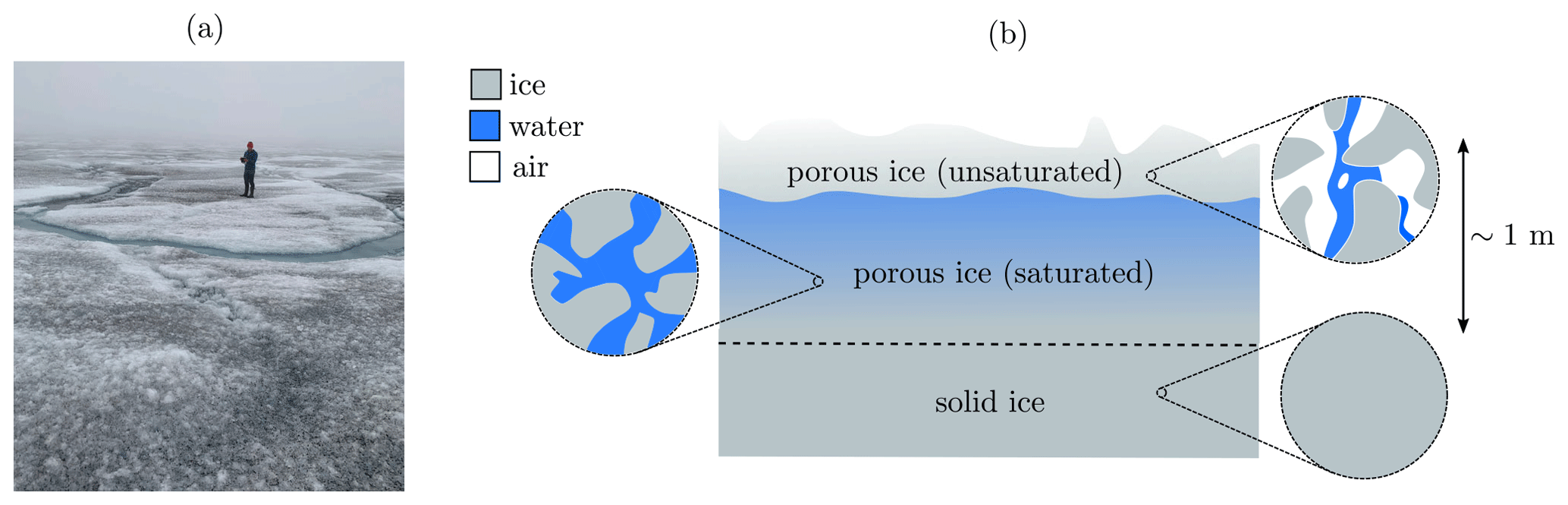
Figure 1 (a) Photo of a weathering crust (credit: Eva Doting). (b) Schematic of a weathering crust – a near-surface layer of porous ice (above the dashed line), below which the ice is impermeable (though the “solid” ice shown here may contain small, closed-off air bubbles). The porosity of the weathering crust decreases with depth. Much of it is saturated with meltwater, with a thin unsaturated layer at the surface. The saturated layer is known as the “weathering crust aquifer”. Schematic based on Cooper et al. (2018); Moure et al. (2022).

The weathering crust is home to many microorganisms, including dark-coloured glacier ice algae at the surface (following the naming convention recommended by Cook et al., 2019, and Hotaling et al., 2021) and algae and bacteria in the weathering crust aquifer (Irvine-Fynn et al., 2021). The growth and transport of these microbes affects the cycling of nutrients such as carbon (e.g. Stibal et al., 2012) and nitrogen (e.g. Telling et al., 2012). For example, microbial activity affects whether an ice-sheet surface is a source or a sink of CO₂, and microbes and nutrients can be transported by the flow of meltwater, impacting downstream habitats such as oceans and soils (Stibal et al., 2012).

The weathering crust can transiently store meltwater and affect how the water is transported across the ice-sheet surface (Cooper et al., 2018). Moreover, the presence of the weathering crust can affect the amount of meltwater produced, since it modulates how much shortwave radiation is reflected or absorbed by the ice. For example, the weathering crust reflects more radiation than the glazed, bare ice left behind when the crust is removed (Tedstone et al., 2020).

In addition to changes to the ice-sheet surface, biological factors – including glacier ice algae (Benning et al., 2014) – contribute to the darkening of the Greenland ice sheet (Hotaling et al., 2021), lowering the albedo and increasing melting. Work has been done to assess and quantify the contribution of glacier ice algae to albedo and surface runoff (e.g. Cook et al., 2017, 2020; Tedstone et al., 2020; Chevrollier et al., 2022). For example, Cook et al. (2020) estimated that 10 %–13 % of the total runoff from south-western Greenland in summer 2017 could be attributed to algae growth. However, it is difficult to isolate the biological impact from the impact due to changes to the weathering crust structure, as well as other factors including non-biological impurities (Tedesco et al., 2016; Cook et al., 2017; Tedstone et al., 2020). The potential positive feedback loop associated with glacier ice algae and melting, whereby increased melting enables more algal growth, demonstrates the intrinsic link between the structure of the weathering crust and the microbial activity within it (Tedstone et al., 2020; McCutcheon et al., 2021). All of this emphasises the need to understand the microbial community and the ice structure as one.

In this paper, we develop a continuum model for the evolution of the weathering crust, to which we couple a model for microbes and nutrients in the weathering crust aquifer. We reduce our model to one dimension and focus on steadily melting solutions in which constant radiation and atmospheric conditions cause the surface to lower at a constant rate. We investigate how the structure of the weathering crust, the amount of melting, and the amount and distribution of microbes are affected by the forcing conditions. In Sect. 2 we describe the model in the absence of any microbes, and we discuss solutions for the weathering crust structure. In Sect. 3 we extend the model to include microbes and nutrients and discuss solutions for the microbial and nutrient distributions as well as the influence of radiative forcings. In Sect. 4, we use our model to investigate feedbacks between microbial growth, albedo, and melting. Finally, in Sect. 5 we discuss our results and conclude.

2 Weathering crust model

2.1 Model

Firstly, we present a model for the evolution of the structure of the weathering crust without any microbes or nutrients present. We use a continuum model, in contrast to the layer model used by Schuster (2001) – the only existing attempt to model the weathering crust that we are aware of. We model the weathering crust as porous ice with upper surface z=h(t). The pores can contain both water and air. The ice takes up a volume fraction 1−ϕ, where ϕ is the porosity. The saturation S describes the proportion of the pore space taken up by water, so ϕS is the volume fraction of water and ϕ(1−S) is the volume fraction of air. The porosity and saturation can evolve by the ice melting internally at a rate m_int (with negative m_int corresponding to water freezing in the pores) and by the water flowing through the porous ice. The internal melting is driven by shortwave (solar) radiation penetrating below the ice surface. We now present the governing equations.

2.1.1 Mass conservation

Mass conservation equations for the ice, water, and air, respectively, are

$$\begin{array}{}\text{(1)}& {\displaystyle \frac{\partial }{\partial t}}\left(\right(\mathrm{1}-\mathit{\varphi }\left){\mathit{\rho }}_{\mathrm{i}}\right)+\mathrm{\nabla }\cdot \left(\right(\mathrm{1}-\mathit{\varphi }\left){\mathit{\rho }}_{\mathrm{i}}{\mathit{u}}_{\mathrm{i}}\right)=-m_{\mathrm{int}},\text{(2)}& {\displaystyle \frac{\partial }{\partial t}}\left(\mathit{\varphi }S{\mathit{\rho }}_{\mathrm{w}}\right)+\mathrm{\nabla }\cdot \left(\mathit{\varphi }S{\mathit{\rho }}_{\mathrm{w}}{\mathit{u}}_{\mathrm{w}}\right)=m_{\mathrm{int}},\text{(3)}& {\displaystyle \frac{\partial }{\partial t}}\left(\mathit{\varphi }\right(\mathrm{1}-S\left){\mathit{\rho }}_{\mathrm{a}}\right)+\mathrm{\nabla }\cdot \left(\mathit{\varphi }\right(\mathrm{1}-S\left){\mathit{\rho }}_{\mathrm{a}}{\mathit{u}}_{\mathrm{a}}\right)=\mathrm{0},\end{array}$$

where ρ_i, ρ_w, and ρ_a are the densities of ice, water, and air, respectively, and u_i, u_w, and u_a are their velocities. Since air is much less dense than ice and water (${\mathit{\rho }}_{\mathrm{a}}\ll {\mathit{\rho }}_{\mathrm{i}},{\mathit{\rho }}_{\mathrm{w}}$), we can neglect Eq. (3). A relationship between the ice and water velocities could come from Darcy's law for flow through a porous medium, and u_i could be prescribed to account for the upward advection of ice in the ablation zone. However, for our purposes in this study, we will later set both u_i and u_w to zero for the specific one-dimensional solution we consider.

2.1.2 Energy equation

We also need to model the temperature T, which we assume to be homogeneous across the ice–water–air mixture. We assume that if water is present ($\mathit{\varphi }>\mathrm{0},S>\mathrm{0}$) then the region is at the melting temperature T_m. If there is no water present (S=0), then the ice can be below the melting temperature T≤T_m.

Conservation of energy leads to the following equation:

$$\begin{array}{}\text{(4)}& \begin{array}{rl}{\displaystyle \frac{\partial }{\partial t}}& \left[\left((\mathrm{1}-\mathit{\varphi }){\mathit{\rho }}_{\mathrm{i}}{c}_{\mathrm{i}}+\mathit{\varphi }S{\mathit{\rho }}_{\mathrm{w}}{c}_{\mathrm{w}}\right)T\right]\\ & +\mathrm{\nabla }\cdot \left[\left((\mathrm{1}-\mathit{\varphi }){\mathit{\rho }}_{\mathrm{i}}{c}_{\mathrm{i}}{\mathit{u}}_{\mathrm{i}}+\mathit{\varphi }S{\mathit{\rho }}_{\mathrm{w}}{c}_{\mathrm{w}}{\mathit{u}}_{\mathrm{w}}\right)T\right]\\ & =\mathrm{\nabla }\cdot \left[\left(k_{\mathrm{i}}(\mathrm{1}-\mathit{\varphi })+k_{\mathrm{w}}\mathit{\varphi }S\right)\mathrm{\nabla }T\right]-\mathrm{\nabla }\cdot \mathit{F}-\mathcal{L}{m}_{\mathrm{int}}.\end{array}\end{array}$$

The terms on the left-hand side represent the rate of change and advection of heat energy. The terms on the right-hand side correspond to heat conduction according to Fourier's law, the heat source provided by internal shortwave radiation F (discussed further below), and the energy available for melting the ice. Here, c_i and c_w are the specific heat capacities and k_i and k_w are the thermal conductivities for ice and water, respectively, and ℒ is the latent heat of fusion of water. Consistent with assuming negligible density of air, we ignore both the heat content and the conductive heat flux in the air. We have assumed a simple volume averaging for the effective thermal conductivity of the combined ice–water mixture.

The energy equation captures two cases. Firstly, when the system is below the melting temperature (T<T_m), there cannot be any internal melting (m_int=0) and there is no water present (S=0). The energy Eq. (4) determines the temperature. Alternatively, when the system is at the melting temperature (T=T_m), melting is possible (m_int≥0) and water can be present (S≥0). Since we know that T=T_m, the energy Eq. (4) instead determines the internal melt rate m_int.

2.1.3 Radiation model

The internal melting of the ice is caused by some of the shortwave radiation from the sun penetrating and being absorbed below the surface of the ice, acting as an internal heat source. We model the internal shortwave radiation flux F following the two-stream approximation (e.g. Perovich, 1990; Liston et al., 1999; Taylor and Feltham, 2004, 2005). We assume that the net radiation flux can be decomposed into upward F₊ and downward F₋ travelling components. The net radiation flux is then $\mathit{F}=(F_{+}-F_{-})\widehat{\mathit{k}}$, where $\widehat{\mathit{k}}$ is the upward-pointing unit vector, with F_± satisfying

$$\begin{array}{}\text{(5)}& {\displaystyle \frac{\partial F_{+}}{\partial z}}=-(\mathit{\alpha }+r)F_{+}+r{F}_{-},\text{(6)}& {\displaystyle \frac{\partial F_{-}}{\partial z}}=(\mathit{\alpha }+r)F_{-}-r{F}_{+},\end{array}$$

where α and r are absorption and scattering coefficients, respectively, with $\mathit{\alpha },r>\mathrm{0}$. We assume that α and r represent bulk properties of the ice–water mixture and, for now, we also assume that α and r are constant. These equations tell us that, as we move through the ice, F₊ is decreased by some of this radiation being absorbed and reflected but increased by some of F₋ being reflected (and thus changing from a downward to an upward flux). A similar argument applies for F₋.

2.1.4 Kinematic conditions

The kinematic conditions for the ice and the water at the surface z=h(t) are, respectively,

$$\begin{array}{}\text{(7)}& {\displaystyle }{\mathit{\rho }}_{\mathrm{i}}(\mathrm{1}-\mathit{\varphi })\left({\mathit{u}}_{\mathrm{i}}\cdot \widehat{\mathit{k}}-\dot{h}\right)={\mathit{\rho }}_{\mathrm{w}}{m}_{\mathrm{surf}}\text{at}z=h\left(t\right),\text{(8)}& {\displaystyle }{\mathit{\rho }}_{\mathrm{w}}\mathit{\varphi }\left({\mathit{u}}_{\mathrm{w}}\cdot \widehat{\mathit{k}}-\dot{h}\right)={\mathit{\rho }}_{\mathrm{w}}(r_{\mathrm{off}}-m_{\mathrm{surf}})\text{at}z=h\left(t\right),\end{array}$$

where ${\mathit{u}}_{\mathrm{i}}\cdot \widehat{\mathit{k}}$ and ${\mathit{u}}_{\mathrm{w}}\cdot \widehat{\mathit{k}}$ are the upward ice and water velocities (which, in the case of water, we expect to be negative), $\dot{h}=\mathrm{d}h/\mathrm{d}t$ is the velocity of the surface, m_surf is the rate of surface melting, and r_off is the rate of runoff.

We assume that any water at the surface drains down into the ice below, provided that the ice is unsaturated. If the surface becomes saturated, we assume that any excess water immediately runs off. In reality, this must be assumed to happen via horizontal flow to other parts of the ice surface and ultimately into the ocean. The runoff term r_off is therefore only non-zero when the surface is saturated.

2.1.5 Surface energy balance

The energy balance at the surface z=h(t) is (see, for example, Hoffman et al., 2008; van den Broeke et al., 2008, 2011)

$$\begin{array}{}\text{(9)}& \begin{array}{rl}-\left(\right(\mathrm{1}-\mathit{\varphi })k_{\mathrm{i}}& +\mathit{\varphi }S{k}_{\mathrm{w}}){\displaystyle \frac{\partial T}{\partial z}}+\mathit{\chi }(\mathrm{1}-a)Q_{\mathrm{si}}-\mathit{ϵ}\mathit{\sigma }{T}^{\mathrm{4}}+Q_{\mathrm{li}}\\ & +C(T_{\mathrm{a}}-T)={\mathit{\rho }}_{\mathrm{w}}\mathcal{L}{m}_{\mathrm{surf}}\mathrm{at}z=h\left(t\right),\end{array}\end{array}$$

where the terms in order from left to right represent conduction of heat from the porous ice, incoming shortwave radiation absorbed at the surface (Q_si is the incoming shortwave (solar) radiation, a is the albedo, χ is the proportion of the total shortwave radiation absorbed by the ice which is absorbed at the surface, discussed further below), emitted longwave radiation given by the Stefan–Boltzmann law for a black body (ϵ is the surface emissivity, a correction for the fact that the ice is not a true black body, and σ is the Stefan–Boltzmann constant), incoming longwave radiation (for example, from reflection off clouds), turbulent heat transfer (C is a turbulent heat transfer coefficient, and T_a is the reference air temperature 2 m above the ice surface), and latent heat flux available for surface melting at rate m_surf.

The turbulent heat flux term takes into account the fact that, if the air is warmer than the surface, winds can cause turbulent eddies that transfer heat from the air to the surface. For simplicity, we are neglecting latent heat transfer due to evaporation and ablation since van den Broeke et al. (2008, 2011) showed this contribution to be small compared to the other terms, at least in the ablation zone of the western Greenland ice sheet.

Often, it is assumed that shortwave radiation incident on an ice-sheet surface is either absorbed at the surface or reflected straight back out, with no radiation being transmitted below the surface. This assumption results in a (1−a)Q_si term in the surface energy balance. However, a key part of weathering crust formation is the penetration of shortwave radiation below the ice surface. Hence, based on methods used by Hoffman et al. (2014) and Law et al. (2020), we introduce the parameter χ<1 – the proportion of the total amount of shortwave radiation absorbed by the ice which is absorbed at the surface – to allow some of the shortwave radiation to penetrate into the subsurface ice, where we model it explicitly as the internal shortwave radiation flux F (see discussion around Eqs. 5 and 6). In particular, this means that the downward internal radiation flux F₋ at the surface z=h(t) is $(\mathrm{1}-\mathit{\chi }(\mathrm{1}-a\left)\right)Q_{\mathrm{si}}$. The upward flux F₊ is aQ_si. Note that in this model the albedo a is not an independent parameter. It is a result of the internal radiation calculation, dependent on the scattering and absorption coefficients α and r (see Sect. 2.3).

By linearising about the melting temperature, the surface energy balance can be re-written as

$$\begin{array}{}\text{(10)}& \begin{array}{rl}-\left(\right(\mathrm{1}-\mathit{\varphi })k_{\mathrm{i}}& +\mathit{\varphi }{k}_{\mathrm{w}}){\displaystyle \frac{\partial T}{\partial z}}+\mathit{\chi }(\mathrm{1}-a)Q_{\mathrm{si}}+Q_{\mathrm{0}}\\ & -\mathit{\upsilon }(T-T_{\mathrm{m}})={\mathit{\rho }}_{\mathrm{w}}\mathcal{L}{m}_{\mathrm{surf}}\mathrm{at}z=h\left(t\right),\end{array}\end{array}$$

where $Q_{\mathrm{0}}=Q_{\mathrm{li}}-\mathit{ϵ}\mathit{\sigma }{T}_{\mathrm{m}}^{\mathrm{4}}+C(T_{\mathrm{a}}-T_{\mathrm{m}})$ is a combination of longwave radiation and turbulent heat flux, which we will prescribe as a function of time, and $\mathit{\upsilon }=C+\mathrm{4}\mathit{ϵ}\mathit{\sigma }{T}_{\mathrm{m}}^{\mathrm{3}}$ is an effective heat transfer coefficient, combining turbulence and radiation.

2.1.6 Model summary

The full weathering crust model is given by the mass conservation Eqs. ( 1) and (2) for ice and water, the energy Eq. (4), and the two-stream Eqs. (5) and (6) for the internal shortwave radiation, along with a prescription of the ice and water velocities u_i and u_w and suitable boundary conditions. As well as the kinematic conditions in Eqs. (7) and (8), the surface energy balance Eq. (10), and the condition for downward-travelling radiation F₋ at the surface, we also require a condition on the upward-travelling radiation F₊ and the temperature T in the far-field (discussed below). The incoming shortwave radiation Q_si and the “other” surface radiation Q₀ (a combination of longwave radiation and turbulent heat fluxes) are prescribed functions of time, representing the climate forcing. In addition to the temperature T, porosity ϕ, and saturation S, additional outputs from the model are the surface and internal melt rates, m_surf and m_int, and surface runoff, r_off. The default parameter values used in the model are shown in Table 1.

Table 1 Default values of the parameters in the model. Unless otherwise stated, these are the parameter values used.

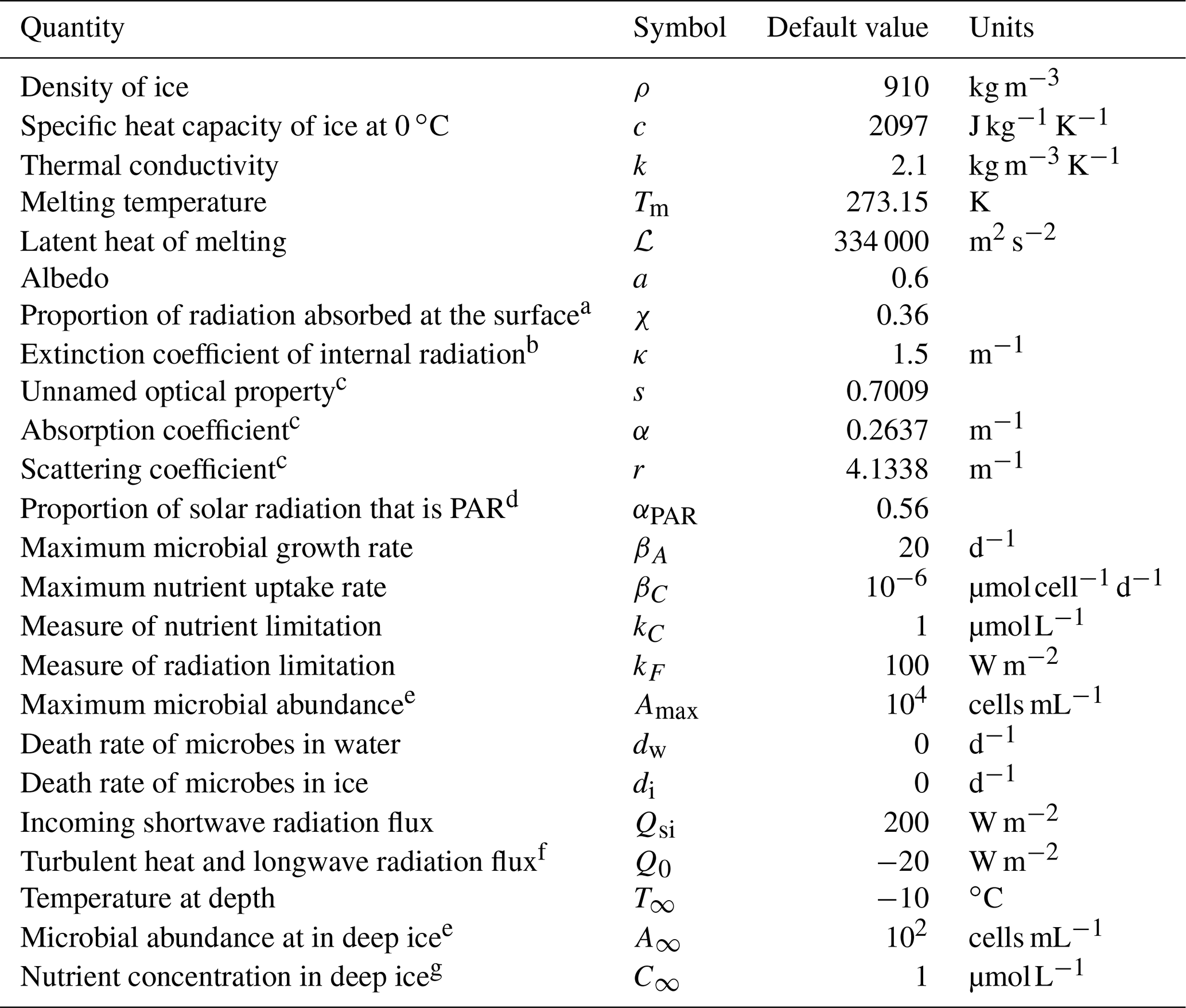
^a Motivated by Hoffman et al. (2014). ^b Taylor and Feltham (2005). ^c Calculated from κ, a, and χ using Eq. (24) and definitions of κ and s. ^d Jørgensen and Bendoricchio (2001). ^e Motivated by Christner et al. (2018). ^f Inferred from van den Broeke et al. (2011). ^g Motivated by Holland et al. (2019). Many of the ice properties are taken from Cuffey and Paterson (2010).

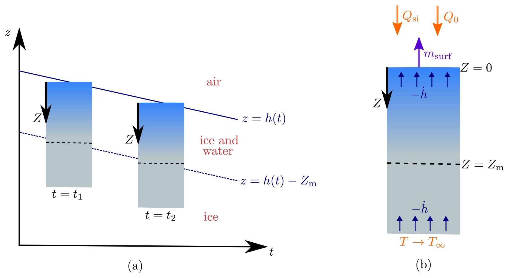
Figure 2 Schematic of the steadily melting setup. Panel (a) shows how the surface of the ice z=h(t) lowers over time in the steadily melting state, with the ice melting in such a way that it looks like the ice column is simply being translated downwards. Panel (b) shows this column of ice in the $Z=h\left(t\right)-z$ frame. The forcings Q_si, Q₀, and T_∞ and the surface melt rate m_surf are also shown.

2.2 Steadily melting states

We now make some simplifications to our model. Firstly, we make the approximation that the ice and water have the same properties, introducing a shared density $\mathit{\rho }={\mathit{\rho }}_{\mathrm{i}}={\mathit{\rho }}_{\mathrm{w}}$, thermal conductivity $k=k_{\mathrm{i}}=k_{\mathrm{w}}$, and specific heat capacity $c=c_{\mathrm{i}}=c_{\mathrm{w}}$. Further, we reduce our model to one dimension considering a vertical column of ice. We also assume that the porous ice is saturated (S=1) and that there is no flow of ice or water (${\mathit{u}}_{\mathrm{i}}={\mathit{u}}_{\mathrm{w}}=\mathbf{0}$). Some of these simplifications could quite easily be relaxed but implementing them allows for a more transparent interpretation of the model solutions.

We now seek what we will refer to as “steadily melting” solutions. These are solutions in which the surface is lowering at a constant rate ($-\dot{h}$), with the subsurface ice melting at exactly a rate m_int to maintain a steady porosity profile below the surface. Therefore, relative to the surface, the solution looks the same at each snapshot in time, as if the column of porous ice is simply being translated downwards, as shown in Fig. 2a. However, this effect is produced by internal and surface melting, not by the ice moving (recall that the ice velocity is zero, by assumption; in reality the downward melting of the ice surface may be counteracted by the upward advection of ice from the interior of the ice sheet). The steadily melting states correspond to an equilibrium between internal melting and surface lowering, which Schuster (2001) observed can occur on cloudy days when the crust is transitioning between growth and decay. It is not expected that this equilibrium lasts long; the weathering crust is very changeable, growing and decaying over a few hours as weather conditions change (Schuster, 2001). Therefore, it would be preferable to have a time-dependent model that can capture this variation. However, for simplicity and to gain some initial insight, we chose to use steady forcings.

The steadily melting setup suggests a natural change of coordinates to

$$\begin{array}{}\text{(11)}& Z=h\left(t\right)-z,\end{array}$$

where Z is the depth below the surface z=h(t) (see Fig. 2). Note that Z points downwards. In the Z frame, the melting surface of the ice is fixed at Z=0, and the ice below gets advected upwards towards the surface at rate $-\dot{h}$, as shown in Fig. 2b. Making this transformation and using the simplifications previously discussed, we can turn our general weathering crust equations into equations for the steadily melting solution. The two-stream Eqs. (5) and (6) for the internal radiation $F=F_{-}-F_{+}$ become

$$\begin{array}{}\text{(12)}& {\displaystyle \frac{\mathrm{d}{F}_{+}}{\mathrm{d}Z}}=(\mathit{\alpha }+r)F_{+}-r{F}_{-},\text{(13)}& {\displaystyle \frac{\mathrm{d}{F}_{-}}{\mathrm{d}Z}}=-(\mathit{\alpha }+r)F_{-}+r{F}_{+}.\end{array}$$

Both the ice and water mass conservation Eqs. (1) and (2) reduce to

$$\begin{array}{}\text{(14)}& \mathit{\rho }\dot{h}{\displaystyle \frac{\mathrm{d}\mathit{\varphi }}{\mathrm{d}Z}}=m_{\mathrm{int}},\end{array}$$

and the energy Eq. (4) becomes

$$\begin{array}{}\text{(15)}& \mathit{\rho }c\dot{h}{\displaystyle \frac{\mathrm{d}T}{\mathrm{d}Z}}=k{\displaystyle \frac{{\mathrm{d}}^{\mathrm{2}}T}{\mathrm{d}{Z}^{\mathrm{2}}}}-{\displaystyle \frac{\mathrm{d}F}{\mathrm{d}Z}}-\mathcal{L}{m}_{\mathrm{int}}.\end{array}$$

The advection terms $\dot{h}\mathrm{d}/\mathrm{d}Z$ come from the time derivatives under the transformation of z→Z. As for boundary conditions, the kinematic conditions (7) and (8) tell us that

$$\begin{array}{}\text{(16)}& -\dot{h}(\mathrm{1}-\mathit{\varphi })=m_{\mathrm{surf}}\mathrm{at}Z=\mathrm{0},\end{array}$$

and that the runoff rate is

$$\begin{array}{}\text{(17)}& r_{\mathrm{off}}=-\dot{h}.\end{array}$$

The linearised surface energy balance (10) becomes

$$\begin{array}{}\text{(18)}& k{\displaystyle \frac{\mathrm{d}T}{\mathrm{d}Z}}+\mathit{\chi }(\mathrm{1}-a)Q_{\mathrm{si}}+Q_{\mathrm{0}}=\mathit{\rho }\mathcal{L}{m}_{\mathrm{surf}}\mathrm{at}Z=\mathrm{0},\end{array}$$

where we have used the fact that T=T_m at the surface in order for surface melting to be possible. In addition to these, we also prescribe a cold temperature T_∞<T_m at depth, so

$$\begin{array}{}\text{(19)}& T\to T_{\mathrm{\infty }}\mathrm{as}Z\to \mathrm{\infty }.\end{array}$$

Finally, the boundary conditions for the two-stream Eqs. (12) and (13) become

$$\begin{array}{}\text{(20)}& F_{-}=(\mathrm{1}-\mathit{\chi }(\mathrm{1}-a\left)\right)Q_{\mathrm{si}}\mathrm{at}Z=\mathrm{0},\end{array}$$

and

$$\begin{array}{}\text{(21)}& F_{+}\to \mathrm{0}\mathrm{as}Z\to \mathrm{\infty },\end{array}$$

since we assume there is no source of shortwave radiation at depth. We also have

$$\begin{array}{}\text{(22)}& F_{+}=a{Q}_{\mathrm{si}}\mathrm{at}Z=\mathrm{0},\end{array}$$

which serves to determine the albedo a (which is defined as the overall ratio of the reflected and incident shortwave radiation). Note that in some cases it may be more natural to prescribe the albedo a as a known (i.e. measured) quantity. In this model, the albedo is related to χ, α, and r, so independently prescribing a would mean that one of these other parameters must be prescribed consistently (see Eq. 24 below).

There are three forcings in our model, which we prescribe. These are the incoming shortwave radiation Q_si, the combined longwave radiation and turbulent heat fluxes Q₀, and the temperature of the ice at depth T_∞. The outputs of the model are the internal shortwave radiation F, porosity ϕ and temperature T, the internal melt rate m_int, surface melt rate m_surf, runoff r_off, and rate of change of surface height $-\dot{h}$. We choose values of the forcings such that the surface is melting (m_surf>0) and the deep ice is cold. Therefore, as shown in Fig. 2, we expect there to be a temperate region $\mathrm{0}<Z<Z_{\mathrm{m}}$ near the surface where the ice is porous (ϕ>0) and at the melting temperature (T=T_m). This region is the weathering crust. In Z>Z_m, the ice is solid (ϕ=0) and cold (T<T_m). We refer to Z_m as the weathering crust thickness or the melting depth, which must also be determined by the model. Note that having impermeable, solid ice at Z=Z_m, combined with our assumption that the ice is saturated with water, justifies our assumption of no water flow (u_w=0), at least in the vertical direction. Furthermore, Irvine-Fynn et al. (2021) have observed lateral flow through the weathering crust to be slow (less than about 0.13 m d⁻¹), which somewhat justifies neglecting horizontal water velocities and using a one-dimensional model.

2.3 Results

In the case where we have constant absorption coefficient α, scattering coefficient r, and albedo a, we can find the steadily melting solution analytically. Firstly, the two-stream Eqs. (12) and (13) can be solved with boundary conditions (20) and (21) to find that the internal radiation $F=F_{-}-F_{+}$ decreases exponentially with depth,

$$\begin{array}{}\text{(23)}& F_{-}=(\mathrm{1}-\mathit{\chi }(\mathrm{1}-a\left)\right)Q_{\mathrm{si}}{e}^{-\mathit{\kappa }Z},F_{+}=s{F}_{-},\end{array}$$

where the extinction coefficient κ is related to the absorption and scattering coefficients α and r by $\mathit{\kappa }=\sqrt{{\mathit{\alpha }}^{\mathrm{2}}+\mathrm{2}\mathit{\alpha }r}$ and $s=(\mathit{\kappa }-\mathit{\alpha })/(\mathit{\kappa }+\mathit{\alpha })$ (e.g. Taylor and Feltham, 2004, 2005). The extra boundary condition (22) for F₊ tells us that

$$\begin{array}{}\text{(24)}& a=s(\mathrm{1}-\mathit{\chi }(\mathrm{1}-a\left)\right).\end{array}$$

This is the relationship telling us that we can only prescribe three of α, r, a, and χ (or equivalently, three of κ, s, a, and χ). Using the condition (24), we can eliminate s from F₊ to obtain

$$\begin{array}{}\text{(25)}& F=F_{-}-F_{+}=(\mathrm{1}-a)(\mathrm{1}-\mathit{\chi })Q_{\mathrm{si}}{e}^{-\mathit{\kappa }Z}.\end{array}$$

This is the familiar Beer's law, previously used to model radiation attenuation in sea ice (e.g. Maykut and Untersteiner, 1971) and glaciers (e.g. Kelliher et al., 1996). We chose to use the two-stream approximation to model the internal radiation rather than assuming Beer's law straight away so that our model can later be extended to non-constant absorption and scattering coefficients α and r. We also note that Cooper et al. (2021) recently made observations of the spectral attenuation of light through bare ice on the Greenland ice sheet, observing that attenuation is greater than through pure ice due to the presence of impurities. However, since our model considers a single band of wavelengths of radiation, we choose to follow Taylor and Feltham (2005) in using κ=1.5 m⁻¹. This is towards the lower end of the range of values observed by Cooper et al. (2021) (∼0.9–8 m⁻¹ for 350–750 nm), but it is at least in the right ballpark.

We can now analytically solve for the steadily melting temperature T, porosity ϕ, and internal melt rate m_int. As mentioned previously, we seek solutions with a temperate region $\mathrm{0}<Z<Z_{\mathrm{m}}$ above a cold region Z>Z_m. The boundary conditions between the two regions are

$$\begin{array}{}\text{(26)}& \mathit{\varphi }=\mathrm{0},T=T_{\mathrm{m}},{\displaystyle \frac{\mathrm{d}T}{\mathrm{d}Z}}=\mathrm{0}\mathrm{at}Z=Z_{\mathrm{m}},\end{array}$$

where the final condition comes from continuity of conductive heat flux. Also, since T=T_m everywhere in $\mathrm{0}<Z<Z_{\mathrm{m}}$, there is no conductive heat flux at the surface, so the surface energy balance Eq. (18) directly tells us the surface melt rate:

$$\begin{array}{}\text{(27)}& m_{\mathrm{surf}}={\displaystyle \frac{\mathit{\chi }(\mathrm{1}-a)Q_{\mathrm{si}}+Q_{\mathrm{0}}}{\mathit{\rho }\mathcal{L}}}.\end{array}$$

In the cold region, we integrate the temperature Eq. (4) and apply the far-field condition (19), along with the fact that a uniform far-field temperature means that the heat flux tends to zero, to obtain

$$\begin{array}{}\text{(28)}& \mathit{\rho }c\dot{h}T-k{\displaystyle \frac{\mathrm{d}T}{\mathrm{d}Z}}+F=\mathit{\rho }c\dot{h}{T}_{\mathrm{\infty }},\end{array}$$

for Z>Z_m. Evaluating this at Z=Z_m and using the boundary conditions (26) gives us an expression which can be rearranged to tell us Z_m in terms of $\dot{h}$:

$$\begin{array}{}\text{(29)}& Z_{\mathrm{m}}=-{\displaystyle \frac{\mathrm{1}}{\mathit{\kappa }}}\log \left({\displaystyle \frac{-\mathit{\rho }c\dot{h}(T_{\mathrm{m}}-T_{\mathrm{\infty }})}{(\mathrm{1}-\mathit{\chi })(\mathrm{1}-a)Q_{\mathrm{si}}}}\right).\end{array}$$

The expression (28) can be integrated once more using the boundary condition (26) for T to find that the temperature is

$$\begin{array}{}\text{(30)}& T=\left\{\begin{array}{l}{T}_{\mathrm{m}},\mathrm{0}<Z<Z_{\mathrm{m}},\\ T_{\mathrm{m}}-\frac{(\mathrm{1}-\mathit{\chi })(\mathrm{1}-a)Q_{\mathrm{si}}}{k\mathit{\kappa }+\mathit{\rho }c\dot{h}}\cdot (e^{-\mathit{\kappa }Z}-e^{-\mathit{\kappa }{Z}_{\mathrm{m}}}{e}^{\frac{\mathit{\rho }c\dot{h}}{k}(Z-Z_{\mathrm{m}})})\\ +T_{\mathrm{\infty }}(\mathrm{1}-e^{\frac{\mathit{\rho }c\dot{h}}{k}(Z-Z_{\mathrm{m}})}),Z>Z_{\mathrm{m}}.\end{array}\right.\end{array}$$

In the temperate region, the energy Eq. (15) determines the internal melt rate m_int from the internal radiation F as follows:

$$\begin{array}{}\text{(31)}& m_{\mathrm{int}}=\left\{\begin{array}{ll}{\displaystyle \frac{\mathit{\kappa }(\mathrm{1}-\mathit{\chi })(\mathrm{1}-a)Q_{\mathrm{si}}}{\mathcal{L}}}{e}^{-\mathit{\kappa }Z},& \mathrm{0}<Z<Z_{\mathrm{m}},\\ \mathrm{0},& Z>Z_{\mathrm{m}}.\end{array}\right.\end{array}$$

In turn, ϕ can be calculated from m_int using the mass conservation Eq. (14), giving

$$\begin{array}{}\text{(32)}& \mathit{\varphi }=\left\{\begin{array}{ll}-\frac{(\mathrm{1}-\mathit{\chi })(\mathrm{1}-a)Q_{\mathrm{si}}}{\mathit{\rho }\dot{h}\mathcal{L}}(e^{-\mathit{\kappa }Z}-e^{-\mathit{\kappa }{Z}_{\mathrm{m}}}),& \mathrm{0}<Z<Z_{\mathrm{m}},\\ \mathrm{0},& Z>Z_{\mathrm{m}}.\end{array}\right.\end{array}$$

Finally, the kinematic condition (16) determines the rate of change of surface height $\dot{h}$ as follows:

$$\begin{array}{}\text{(33)}& \dot{h}=-{\displaystyle \frac{(\mathrm{1}-a)Q_{\mathrm{si}}+Q_{\mathrm{0}}}{\mathit{\rho }\mathcal{L}+\mathit{\rho }c(T_{\mathrm{m}}-T_{\mathrm{\infty }})}},\end{array}$$

which can be substituted into the expression (29) for the melting depth to give

$$\begin{array}{}\text{(34)}& Z_{\mathrm{m}}={\displaystyle \frac{\mathrm{1}}{\mathit{\kappa }}}\log \left(\right({\displaystyle \frac{(\mathrm{1}-a)(\mathrm{1}-\mathit{\chi })Q_{\mathrm{si}}}{\mathit{\rho }c(T_{\mathrm{m}}-T_{\mathrm{\infty }})}})/({\displaystyle \frac{(\mathrm{1}-a)Q_{\mathrm{si}}+Q_{\mathrm{0}}}{\mathit{\rho }\mathcal{L}+\mathit{\rho }c(T_{\mathrm{m}}-T_{\mathrm{\infty }})}}\left)\right).\end{array}$$

As is automatic from Eq. (17), the surface runoff in this situation is equal to the rate of surface lowering, $r_{\mathrm{off}}=-\dot{h}$. Example solutions for temperature, porosity, internal radiation, and internal melt rate are shown in Fig. 3 for two different values of the deep-ice temperature T_∞. Unsurprisingly, a colder deep-ice temperature (blue lines) leads to a smaller porous region, with the dotted lines indicating Z=Z_m.

Figure 3 Example solution for $T_{\mathrm{\infty }}=-\mathrm{10}$ ^∘C (dark blue) and $T_{\mathrm{\infty }}=-\mathrm{1}$ ^∘C (grey). The dotted lines show the melting depth Z_m, with Z_m≈1.8 m when $T_{\mathrm{\infty }}=-\mathrm{10}$ ^∘C and Z_m≈3.3 m when $T_{\mathrm{\infty }}=-\mathrm{1}$ ^∘C. The rate of change in surface height is $\dot{h}\approx -\mathrm{1.6}$ cm d⁻¹ when $T_{\mathrm{\infty }}=-\mathrm{10}$ ^∘C and $\dot{h}\approx -\mathrm{1.7}$ cm d⁻¹ when $T_{\mathrm{\infty }}=-\mathrm{1}$ ^∘C. The surface melt rate is m_surf≈0.25 cm d⁻¹ in both cases. The other parameter values are those shown in Table 1. The shaded region on the left panel corresponds to the smaller region shown in the other panels.

For our assumption that the surface is melting to be valid, we need the surface melt rate m_surf to be positive. Using the expression (27) for m_surf, this gives a restriction on the possible values of the prescribed radiations Q_si and Q₀,

$$\begin{array}{}\text{(35)}& \mathit{\chi }(\mathrm{1}-a)Q_{\mathrm{si}}+Q_{\mathrm{0}}>\mathrm{0}.\end{array}$$

Furthermore, the solution found here, with a porous ice region occupying $\mathrm{0}<Z<Z_{\mathrm{m}}$, is only valid if the calculated Z_m is positive, and hence the argument of the logarithm in Eq. (34) must be greater than 1. Physically, this can be interpreted as requiring that the raising of the internal temperature dominates the surface lowering, as we will now explain.

Firstly, as more of the internal ice is raised to the melting temperature, the size of the porous region (and hence Z_m) increases. This is represented by the term

$$\begin{array}{}\text{(36)}& {\displaystyle \frac{(\mathrm{1}-a)(\mathrm{1}-\mathit{\chi })Q_{\mathrm{si}}}{\mathit{\rho }c(T_{\mathrm{m}}-T_{\mathrm{\infty }})}},\end{array}$$

in the expression (34) for Z_m. The numerator is the amount of radiation absorbed internally, i.e. the energy available to heat and melt the internal ice. The denominator represents the energy needed to raise the ice temperature from T_∞ at depth to the melting temperature, i.e. the energy required to raise the internal ice to the melting temperature. Therefore, the fraction (36) can be thought of as a measure of raising the internal ice to the melting temperature.

On the other hand, as the surface lowers, the size of the porous region (and hence Z_m) decreases, since the porous ice at the surface gets removed as meltwater. Surface lowering is represented by the term

$$\begin{array}{}\text{(37)}& {\displaystyle \frac{(\mathrm{1}-a)Q_{\mathrm{si}}+Q_{\mathrm{0}}}{\mathit{\rho }\mathcal{L}+\mathit{\rho }c(T_{\mathrm{m}}-T_{\mathrm{\infty }})}},\end{array}$$

in the expression (34) for Z_m. The numerator is the total amount of radiation absorbed by the ice, accounting for both internal and surface absorption. This is the total energy available for melting the ice (both at the surface and internally). The denominator represents the energy required to melt cold ice; the temperature must first be raised from T_∞ to T_m, then latent heat is needed to effect the phase change. Indeed, it is this fraction that also gives the surface lowering rate $-\dot{h}$ in Eq. (33). It is different from the surface melt rate m_surf, since melting occurs in two stages: first the ice can melt internally, lowering the porosity, then the remaining ice melts at the surface.

As previously mentioned, we expect Z_m>0 when raising the internal temperature dominates surface lowering. Using the above interpretations of the fractions (36) and (37), this happens when

$$\begin{array}{}\text{(38)}& {\displaystyle \frac{(\mathrm{1}-a)(\mathrm{1}-\mathit{\chi })Q_{\mathrm{si}}}{\mathit{\rho }c(T_{\mathrm{m}}-T_{\mathrm{\infty }})}}>{\displaystyle \frac{(\mathrm{1}-a)Q_{\mathrm{si}}+Q_{\mathrm{0}}}{\mathit{\rho }\mathcal{L}+\mathit{\rho }c(T_{\mathrm{m}}-T_{\mathrm{\infty }})}},\end{array}$$

and Eq. (34) then gives Z_m>0.

The conditions (35) and (38) tell us the range of parameter values for which we can have steadily melting solutions with a non-trivial porous region, i.e. for which a weathering crust exists. Figure 4a illustrates this graphically, showing the range of values of shortwave radiation Q_si and combined longwave radiation and turbulent heat fluxes Q₀ for which the steadily melting states with a non-trivial weathering crust are possible (blue to yellow region). For a fixed amount of shortwave radiation Q_si, increasing the other surface radiation Q₀ increases the amount of surface lowering but not the internal heating. This is because Q₀ is completely absorbed at the surface. If Q₀ is too large, surface lowering is so large that ice gets advected to the surface so quickly that it does not have the chance to get heated up to the melting temperature internally first. Hence there is no internal melting. If Q₀ is too small, there is not enough energy to melt the surface.

Figure 4 (a, b) The range of Q_si and Q₀ values for which steadily melting states with both internal and surface melting are possible, as well as the regions for which there is no surface melting and no internal melting (grey). Contours of (a) rate of surface lowering $-\dot{h}$ and (b) weathering crust thickness Z_m are shown, ranging from $-\dot{h}=\mathrm{0}$ cm d⁻¹ to $-\dot{h}=\mathrm{20}$ cm d⁻¹ and from Z_m=0 m to Z_m=1.9 m with 1 cm d⁻¹ and 0.1 m spacing between contours, respectively. (c) The dependence of Z_m on the shortwave radiation Q_si when Q₀=20 W m⁻², $Q_{\mathrm{0}}=-\mathrm{20}$ W m⁻², and Q₀=0 W m⁻². The other parameter values are those shown in Table 1.

The weathering crust thicknesses Z_m found from our model broadly agree with the ice core measurements taken by Cooper et al. (2018) in the south-western Greenland ice sheet ablation zone. They found the weathering crust in that region to be at least 1 m and up to about 2 m thick, in line with our results in Fig. 4b. Moreover, Fig. 4b and c show how the weathering crust thickness Z_m depends on the incoming shortwave radiation Q_si and the combined longwave radiation and turbulent heat fluxes Q₀. There is a qualitative difference between the behaviour of Z_m with Q_si, depending on the sign of Q₀. We see that Z_m increases with Q_si when Q₀>0 but decreases with Q_si when Q₀<0. The reason for this relates back to our interpretation of Z_m being determined by a balance between internal heating and surface lowering. If Q₀<0, doubling Q_si doubles the internal heating term (36) and more than doubles the surface lowering term (37). Therefore, as Q_si increases, surface lowering becomes more significant compared to internal heating, so the porous region (and hence Z_m) decreases. On the other hand, if Q₀>0, surface lowering becomes less significant as Q_si increases, so the porous region (and hence Z_m) increases. In both cases, a weathering crust can only exist if the shortwave radiation Q_si is large enough. Physically, positive Q₀ corresponds to conditions of warm air temperature, strong wind, and cloud cover, when the ice surface would melt even in the absence of solar radiation. Such conditions favour removal of the weathering crust (Muller and Keeler, 1969; Schuster, 2001), as we observe in Fig. 4 when Q₀ becomes too large. Negative Q₀ corresponds to conditions when the surface would freeze in the absence of solar radiation. In the ablation zone of the western Greenland ice sheet, we would typically expect the net longwave radiation to be negative and the turbulent heat fluxes to be positive, with the combination giving Q₀ as slightly negative (van den Broeke et al., 2008, 2011). An exception is in regions near the margin where ice-free tundra causes positive turbulent heat fluxes to dominate (van den Broeke et al., 2008, 2011). However, the weather conditions on the Greenland ice sheet are very changeable (e.g. Fausto et al., 2021), rapidly changing between clear, sunny conditions that favour weathering crust formation and cloudy, windy, and warm weather that favours removal of the crust (Muller and Keeler, 1969; Schuster, 2001). Therefore, we choose to investigate both positive and negative Q₀ to explore the different behaviours exhibited during these changeable conditions. The sensitivity of the weathering crust thickness Z_m to the values of Q_si and Q₀, demonstrated by our model might partly explain why the weathering crust tends to form and be removed by changing weather conditions.

3 Microbes and nutrients model

3.1 Model

We now extend our model to include microbes and nutrients. Our model focusses on the microbes within the weathering crust aquifer and does not account for the ice algae found right on the ice-sheet surface (see Sect. 5 for further discussion). In order to keep things simple, we model a single “representative” nutrient, the concentration of which influences the microbial growth. In reality, there may be multiple sources of such nutrients located within the modelled space. The microbial growth will also depend on the shortwave radiation flux F. We also model a single representative type of phototrophic microbe (a microbe that obtains energy from solar radiation), rather than separately considering different primary and secondary producers (see discussion in Sect. 5). We assume that both the microbes and the nutrients can exist in both the ice and the water, and when the ice melts they are transferred from the ice to the water. Microbes in the water can consume nutrients from the water but not from the ice, and microbes in the ice cannot consume any nutrients (see Fig. 5). Therefore, only microbes in the water are able to proliferate. We model the microbial abundance of microbes in the water A_w and ice A_i (cells mL⁻¹) separately, and we do the same for the nutrient concentrations C_w and C_i (µmol L⁻¹).

Figure 5 Schematic illustration of how microbes (big purple dots) and nutrients (small pink dots) are included in the model. Both are transferred from ice (grey) to water (blue) as the ice melts (red arrows), and the microbes in the water then consume nutrients in the water (bright blue arrow).

To model the water microbial abundance A_w, we adapt a simple logistic growth model (Murray, 1993),

$$\begin{array}{}\text{(39)}& \begin{array}{rl}{\displaystyle \frac{\partial }{\partial t}}& \left(\mathit{\varphi }{A}_{\mathrm{w}}\right)+\mathrm{\nabla }\cdot \left(\mathit{\varphi }{A}_{\mathrm{w}}{\mathit{u}}_{\mathrm{w}}\right)\\ & =g(F,\mathit{\varphi }{C}_{\mathrm{w}})\mathit{\varphi }{A}_{\mathrm{w}}\left(\mathrm{1}-{\displaystyle \frac{A_{\mathrm{w}}}{A_{max}}}\right)-d_{\mathrm{w}}\mathit{\varphi }{A}_{\mathrm{w}}\\ & +{\displaystyle \frac{A_{\mathrm{i}}}{{\mathit{\rho }}_{\mathrm{i}}}}max(m_{\mathrm{int}},\mathrm{0})-{\displaystyle \frac{A_{\mathrm{w}}}{{\mathit{\rho }}_{\mathrm{w}}}}min(m_{\mathrm{int}},\mathrm{0}).\end{array}\end{array}$$

On the left-hand side, we have the time derivative and an advection term, with the microbes being advected at the water velocity u_w. On the right-hand side we have a growth term, a death term (with a death rate d_w), and source and sink terms due to melting and freezing, respectively. The growth term, of the form $g\mathit{\varphi }{A}_{\mathrm{w}}(\mathrm{1}-A_{\mathrm{w}}/A_{max})$, is the standard form for logistic growth, with A_max being the maximum microbial abundance. We base the form of the logistic growth rate g on that used by Jørgensen and Bendoricchio (2001) for algal growth, in which g depends on the intensity of photosynthetically active radiation, the volume-averaged nutrient concentration ϕC_w and the temperature, since these are limiting factors for growth of photosynthetic microbes. (We can ignore the temperature dependence, since we assume that the water is always at the melting temperature.) We follow Jørgensen and Bendoricchio (2001) in using a Michaelis–Menten form of the growth term,

$$\begin{array}{}\text{(40)}& g(F,\mathit{\varphi }{C}_{\mathrm{w}})={\mathit{\beta }}_A\left({\displaystyle \frac{{\mathit{\alpha }}_{\mathrm{PAR}}F}{k_{\mathrm{PAR}}+{\mathit{\alpha }}_{\mathrm{PAR}}F}}\right)\left({\displaystyle \frac{\mathit{\varphi }{C}_{\mathrm{w}}}{k_C+\mathit{\varphi }{C}_{\mathrm{w}}}}\right),\end{array}$$

where α_PAR=0.56 is the proportion of the total incident solar radiation that is photosynthetically active (i.e. that can be used for photosynthesis). Photosynthesis, like weathering crust formation, is driven by shortwave radiation. Here, the broadband radiation F represents all wavelengths of shortwave radiation. The factor α_PAR accounts for the fact that the two processes in fact use slightly different (overlapping) parts of the spectrum. k_PAR and k_C are constants used to represent the fact that, above a certain limit, increasing the radiation or nutrient concentration further will no longer lead to increased algal growth. β_A is also a constant, which represents the growth rate if there is abundant radiation and nutrients (in which case the two bracketed factors are essentially 1). We refer to β_A as the growth rate constant.

The ice microbial abundance equation is simpler. We assume that the microbes in the ice cannot grow but can die (with a death rate d_i) and are fixed within the ice (so they are advected at the ice velocity u_i). Hence A_i satisfies

$$\begin{array}{}\text{(41)}& \begin{array}{rl}{\displaystyle \frac{\partial }{\partial t}}& \left(\right(\mathrm{1}-\mathit{\varphi }\left)A_{\mathrm{i}}\right)+\mathrm{\nabla }\cdot \left(\right(\mathrm{1}-\mathit{\varphi }\left)A_{\mathrm{i}}{\mathit{u}}_{\mathrm{i}}\right)\\ & =-d_{\mathrm{i}}(\mathrm{1}-\mathit{\varphi })A_{\mathrm{i}}-{\displaystyle \frac{A_{\mathrm{i}}}{{\mathit{\rho }}_{\mathrm{i}}}}max(m_{\mathrm{int}},\mathrm{0})+{\displaystyle \frac{A_{\mathrm{w}}}{{\mathit{\rho }}_{\mathrm{w}}}}min(m_{\mathrm{int}},\mathrm{0}).\end{array}\end{array}$$

We expect that d_i≥d_w, meaning that the death rate of microbes in the ice is greater than the death rate in the water.

Nutrients are transported through the weathering crust aquifer, often from nutrient-rich cryoconite holes (Cook et al., 2016). To model the nutrient transport in the water, we use similar ideas to those used to model bioreactors (e.g. Shakeel et al., 2013). The nutrients in the water can be advected and consumed by microbes. The melting of ice provides a source of nutrients into the water (and a sink from the ice), and water freezing provides a corresponding sink. The nutrients in the ice are advected with the ice but cannot be consumed because microbes cannot access the nutrients in the ice. The equations describing this are

$$\begin{array}{}\text{(42)}& \begin{array}{rl}{\displaystyle \frac{\partial }{\partial t}}& \left(\mathit{\varphi }{C}_{\mathrm{w}}\right)+\mathrm{\nabla }\cdot \left(\mathit{\varphi }{C}_{\mathrm{w}}{\mathit{u}}_{\mathrm{w}}\right)\\ & =-{\mathit{\beta }}_C\mathit{\varphi }{A}_{\mathrm{w}}\left({\displaystyle \frac{{\mathit{\alpha }}_{\mathrm{PAR}}F}{k_{\mathrm{PAR}}+{\mathit{\alpha }}_{\mathrm{PAR}}F}}\right)\left({\displaystyle \frac{\mathit{\varphi }{C}_{\mathrm{w}}}{k_C+\mathit{\varphi }{C}_{\mathrm{w}}}}\right)\\ & +{\displaystyle \frac{C_{\mathrm{i}}}{{\mathit{\rho }}_{\mathrm{i}}}}max(m_{\mathrm{int}},\mathrm{0})-{\displaystyle \frac{C_{\mathrm{w}}}{{\mathit{\rho }}_{\mathrm{w}}}}min(m_{\mathrm{int}},\mathrm{0}),\end{array}\end{array}$$

for the nutrients in the water and

$$\begin{array}{}\text{(43)}& \begin{array}{rl}{\displaystyle \frac{\partial }{\partial t}}& \left(\right(\mathrm{1}-\mathit{\varphi }\left)C_{\mathrm{i}}\right)+\mathrm{\nabla }\cdot \left(\right(\mathrm{1}-\mathit{\varphi }\left)C_{\mathrm{i}}{\mathit{u}}_{\mathrm{i}}\right)\\ & =-{\displaystyle \frac{C_{\mathrm{i}}}{{\mathit{\rho }}_{\mathrm{i}}}}max(m_{\mathrm{int}},\mathrm{0})+{\displaystyle \frac{C_{\mathrm{w}}}{{\mathit{\rho }}_{\mathrm{w}}}}min(m_{\mathrm{int}},\mathrm{0}),\end{array}\end{array}$$

for the nutrients in the ice. The uptake term has a similar form to the growth rate in Eq. (39) since we expect the consumption of nutrients to be related to the growth rate of the microbes. The constant β_C represents a maximum nutrient uptake rate and controls the degree to which microbes influence the nutrient concentration.

A further assumption we make is that microbes and nutrients get instantaneously removed in surface runoff. This would need to be modified if we extended our model to include surface ice algae, which are able to persist on the ice surface, even in the presence of surface runoff (see Sect. 5).

Equations (39), (41), (42), and (43) for the microbial abundances A_w and A_i and nutrient concentrations C_w and C_i are coupled to Eqs. (1), (2), (4), (5), and (6) for the weathering crust evolution since they depend on both porosity ϕ and radiation F.

3.2 Steadily melting equations

We now return to the steadily melting states considered in Sect. 2.2. Under these same assumptions and making the same change of coordinates (11), Eqs. (39) and (42) for the microbial abundance and nutrient concentration in the water become

$$\begin{array}{}\text{(44)}& {\displaystyle }\begin{array}{rl}\dot{h}{\displaystyle \frac{\mathrm{d}}{\mathrm{d}Z}}\left(\mathit{\varphi }{A}_{\mathrm{w}}\right)& ={\mathit{\beta }}_A\mathit{\varphi }{A}_{\mathrm{w}}\left({\displaystyle \frac{{\mathit{\alpha }}_{\mathrm{PAR}}F}{k_{\mathrm{PAR}}+{\mathit{\alpha }}_{\mathrm{PAR}}F}}\right)\cdot \left({\displaystyle \frac{\mathit{\varphi }{C}_{\mathrm{w}}}{k_C+\mathit{\varphi }{C}_{\mathrm{w}}}}\right)\left(\mathrm{1}-{\displaystyle \frac{A_{\mathrm{w}}}{A_{max}}}\right)\\ & -d_{\mathrm{w}}\mathit{\varphi }{A}_{\mathrm{w}}+{\displaystyle \frac{A_{\mathrm{i}}{m}_{\mathrm{int}}}{\mathit{\rho }}},\end{array}\text{(45)}& {\displaystyle }\dot{h}{\displaystyle \frac{\mathrm{d}}{\mathrm{d}Z}}\left(\mathit{\varphi }{C}_{\mathrm{w}}\right)=-{\mathit{\beta }}_C\mathit{\varphi }{A}_{\mathrm{w}}\left({\displaystyle \frac{{\mathit{\alpha }}_{\mathrm{PAR}}F}{k_{\mathrm{PAR}}+{\mathit{\alpha }}_{\mathrm{PAR}}F}}\right)\cdot \left({\displaystyle \frac{\mathit{\varphi }{C}_{\mathrm{w}}}{k_C+\mathit{\varphi }{C}_{\mathrm{w}}}}\right)+{\displaystyle \frac{C_{\mathrm{i}}{m}_{\mathrm{int}}}{\mathit{\rho }}}.\end{array}$$

As an additional simplification, we make the assumption that the microbes in the water and in the ice do not die, so $d_{\mathrm{w}}=d_{\mathrm{i}}=\mathrm{0}$. In this particular situation, Eqs. (41) and (43) for A_i and C_i simply tell us that the microbial abundance and nutrient concentration in the ice are constant. Since we prescribe the microbial abundance and nutrient concentration in the deep ice to be A_∞ and C_∞, respectively, this leads to A_i=A_∞ and C_i=C_∞ everywhere.

Referring back to Fig. 2, water is only present in the porous region $\mathrm{0}<Z<Z_{\mathrm{m}}$, so it is in this region that we solve Eqs. (44) and (45) for A_w and C_w. For continuity at the interface Z=Z_m between the porous ice and the solid ice, we prescribe

$$\begin{array}{}\text{(46)}& {\displaystyle }{A}_{\mathrm{w}}=A_{\mathrm{i}}\mathrm{at}Z=Z_{\mathrm{m}},\text{(47)}& {\displaystyle }{C}_{\mathrm{w}}=C_{\mathrm{i}}\mathrm{at}Z=Z_{\mathrm{m}}.\end{array}$$

For simplicity, we assume for now that absorption of shortwave radiation is independent of microbial abundance (with this assumption being removed in Sect. 4). As a result, the microbe and nutrient problem decouples from the weathering crust problem. The analytical solution to the weathering crust problem found in Sect. 2.3 can first be used to calculate ϕ, m_int, $\dot{h}$, and Z_m. Then, using these results, Eqs. (44) and (45) can be solved (numerically) with the boundary conditions (46) and (47) for A_w and C_w. We do this using the boundary value problem solver bvp4c in MATLAB. Our code is made available at https://doi.org/10.5281/zenodo.7199159(Woods, 2022).

Before looking at some solutions, we discuss what we expect to be typical values of the microbial abundance and nutrient concentrations. Motivated by Christner et al. (2018), we choose $A_{max}={\mathrm{10}}^{\mathrm{4}}$ cells mL⁻¹ and A_∞=10² cells mL⁻¹ as sensible values for the maximum microbial abundance and the microbial abundance deep in the ice. The nutrient concentration deep in the ice C_∞ gives the maximum value of C_w in the steadily melting model. To estimate a value for C_∞, we note that Holland et al. (2019) measured concentrations of dissolved organic and inorganic nitrogen, phosphorous, and carbon near the surface of the Greenland ice sheet dark zone varying in orders of magnitude from about 0.1 µmol L⁻¹ to over 100 µmol L⁻¹. The nutrient concentration of interest will be that of the most limiting nutrient, which could potentially be any of these. Therefore, as a ballpark figure, we take C_∞=1 µmol L⁻¹. In fact, the actual numerical values of nutrient concentration are not particularly important to the model, and we will show the nutrient concentration solutions normalised by C_∞.

3.3 Results

3.3.1 Effect of microbial growth rate

Figure 6 shows an example solution of how the volume-averaged microbial abundance ϕA_w and nutrient concentration ϕC_w vary with depth in the weathering crust shown in Fig. 3. The solutions are shown for two different values of microbial growth rate: β_A=20 d⁻¹ (dark blue line) and β_A=5 d⁻¹ (grey line). The latter value is loosely based on observed doubling times of algal blooms on the Greenland ice sheet (Stibal et al., 2017; Williamson et al., 2018). We note that these observations are of lateral spreading of algal blooms on the ice-sheet surface, not microbial growth within the weathering crust. Therefore, our approximate values of β_A are crude but still serve to demonstrate the key behaviour it is possible to capture with our model. Even in the porous region (above the dotted line showing where Z=Z_m), there is an inner region where the microbial abundance A_w and nutrient concentration C_w are still approximately their deep-ice values, and hence $\mathit{\varphi }{A}_{\mathrm{w}}/A_{max}\approx \mathit{\varphi }{A}_{\mathrm{\infty }}/A_{max}$ (=0.01ϕ) and $\mathit{\varphi }{C}_{\mathrm{w}}/C_{\mathrm{\infty }}\approx \mathit{\varphi }$. Above this, A_w increases towards the surface and C_w decreases. This is because there is more shortwave radiation nearer the surface, enabling more microbial growth. In turn, more microbes mean that more nutrients get consumed. We can see that, as we would expect, there are more microbes when the growth rate is higher (dark blue line). The turning point in the nutrient profiles is the point above which the nutrient concentration C_w changes significantly from the deep-ice value C_∞, causing the bulk nutrient concentration ϕC_w to move off the exponential porosity profile.

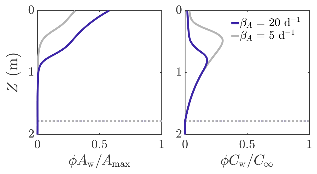
Figure 6 Volume-averaged microbial abundance ϕA_w and nutrient concentration ϕC_w solutions scaled with the maximum concentrations A_max and C_∞. Solutions correspond to the weathering crust solutions (dark blue lines) in Fig. 3. The solutions are shown for β_A=20 d⁻¹ (dark blue line) and β_A=5 d⁻¹ (grey line). The dotted line shows Z=Z_m. The other parameter values are those shown in Table 1.

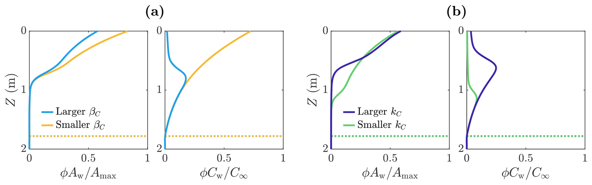
Figure 7 Volume-averaged microbial abundance ϕA_w and nutrient concentration ϕC_w solutions scaled with the maximum concentrations A_max and C_∞. Panel (a) shows the solutions for ${\mathit{\beta }}_C/C_{\mathrm{\infty }}={\mathrm{10}}^{-\mathrm{3}}$ mL cell⁻¹ d⁻¹ (light blue) and ${\mathit{\beta }}_C/C_{\mathrm{\infty }}={\mathrm{10}}^{-\mathrm{5}}$ mL cell⁻¹ d⁻¹ (yellow). Panel (b) shows the solutions for k_C=2C_∞ (dark blue) and k_C=0.2C_∞ (green). These solutions correspond to the weathering crust solutions (dark blue lines) in Fig. 3. The dotted lines show the melting depth Z_m≈1.78 m. The other parameter values are those shown in Table 1.

3.3.2 Effect of nutrient parameters

We now investigate how the distribution of microbes is affected by parameters related to the uptake of the nutrient. In particular, we look at the parameters β_C and k_C. Firstly, β_C is the maximum nutrient uptake rate, with a larger value of β_C meaning that the microbes consume more nutrients to achieve the same amount of growth. Figure 7a shows the distribution of microbial abundance A_w and nutrient concentration C_w with depth for two values of β_C – one 100 times larger (light blue) than the other (yellow). Consistent with our interpretation of β_C, the nutrient concentration C_w is lower when β_C is larger. Correspondingly, the microbial abundance A_w is lower because the nutrient has been used up more quickly by the microbes, so less nutrient is available for further microbial growth.

The second nutrient parameter k_C is a measure of the point at which the nutrient stops being a limiting factor for the microbes. The larger k_C is, the higher the volume-averaged nutrient concentration ϕC_w must be before the microbial growth rate becomes independent of ϕC_w. Equivalently, the smaller k_C is, the lower the volume-averaged nutrient concentration must get before the nutrient becomes a limiting factor. Figure 7b shows the distribution of microbial abundance A_w and nutrient concentration C_w with depth for two values of k_C – one 10 times larger (dark blue) than the other (green). The effect of decreasing k_C is to increase the size of the region in which there is a significant number of microbes. This is because the porosity decreases with depth, which in turn means the volume-averaged nutrient concentration ϕC_w decreases with depth in the region near Z=Z_m where C_w≈C_∞. Therefore, as k_C becomes smaller, the depth at which the nutrient becomes a limiting factor (controlled by the size of ϕC_w relative to k_C) increases, so the microbes spread deeper into the ice. Note that decreasing β_C does not affect the depth to significant microbial growth because the size of β_C does not change the conditions required for microbial growth – it only affects the rate at which nutrients are consumed.

3.3.3 Total microbial abundance

As we did for the weathering crust, we can examine how the steadily melting solution varies with radiative forcing, assuming fixed microbe and nutrient parameters. Firstly, we show solutions for different Q₀ and Q_si in Fig. 8. Secondly, we look at the dependence of the total amount of microbes in the water A_tot,w, defined as

$$\begin{array}{}\text{(48)}& A_{\mathrm{tot},\mathrm{w}}=\underset{\mathrm{0}}{\overset{Z_{\mathrm{m}}}{\int }}\mathit{\varphi }{A}_{\mathrm{w}}\mathrm{d}Z.\end{array}$$

This has units of cells m⁻². As discussed at the end of Sect. 2.3, changing weather conditions (represented by the radiative forcings Q_si and Q₀ in our model) lead to the formation and removal of the weathering crust. Therefore, we choose to investigate the response of microbes to changes in both Q_si and Q₀, including positive and negative Q₀, to capture the range of conditions experienced by microbes in the weathering crust. For a weathering crust to form, the shortwave radiation Q_si must be large enough. Positive Q₀ corresponds to conditions of high turbulent heat flux (warm, cloudy, windy), which promote removal of the weathering crust. Negative Q₀ means that the surface would freeze in the absence of shortwave radiation. The observed behaviour is quite different in these two cases.

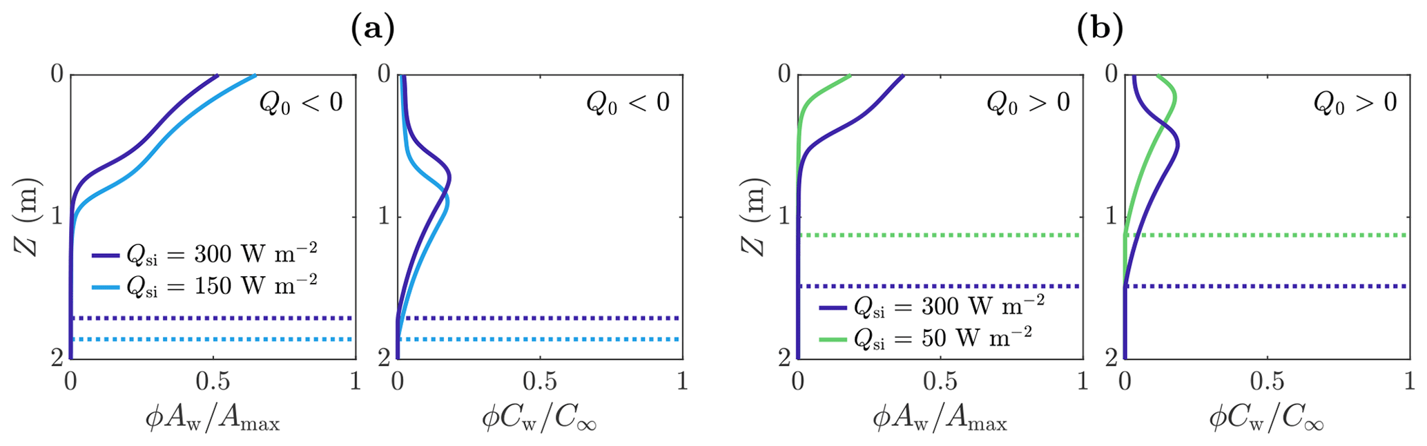
Figure 8 The effect of Q_si and Q₀ on volume-averaged microbial abundance ϕA_w and nutrient concentration ϕC_w solutions scaled with the maximum concentrations A_max and C_∞. Panel (a) shows the solutions for $Q_{\mathrm{0}}=-\mathrm{20}$ W m⁻² (negative) in the case of Q_si=150 W m⁻² (light blue) and Q_si=300 W m⁻² (dark blue). Panel (b) shows the solutions for Q₀=20 W m⁻² (positive) in the case of Q_si=50 W m⁻² (green) and Q_si=300 W m⁻² (dark blue). The dotted lines show the weathering crust thickness Z_m. The other parameter values are those shown in Table 1.

Figure 9a shows that when Q₀>0 and for small values of Q_si – below the critical value required to produce internal melting – there are no water microbes because there is no water. Then, as Q_si increases, A_tot,w increases due to the increase in internal radiation leading to an increase in microbial growth and an increase in the size of the weathering crust Z_m (i.e. the region in which microbes can grow). As shown in Fig. 9c, if Q_si is increased further (to less physical values), the total amount of microbes A_tot,w starts to decrease again. This is because the internal radiation reaches the level above which it is no longer a limiting factor for the microbes. Increasing the shortwave radiation further does not increase the microbial growth but does continue to increase the surface lowering and runoff, meaning that the removal of microbes in runoff begins to dominate microbial growth, causing a reduction in A_tot,w.

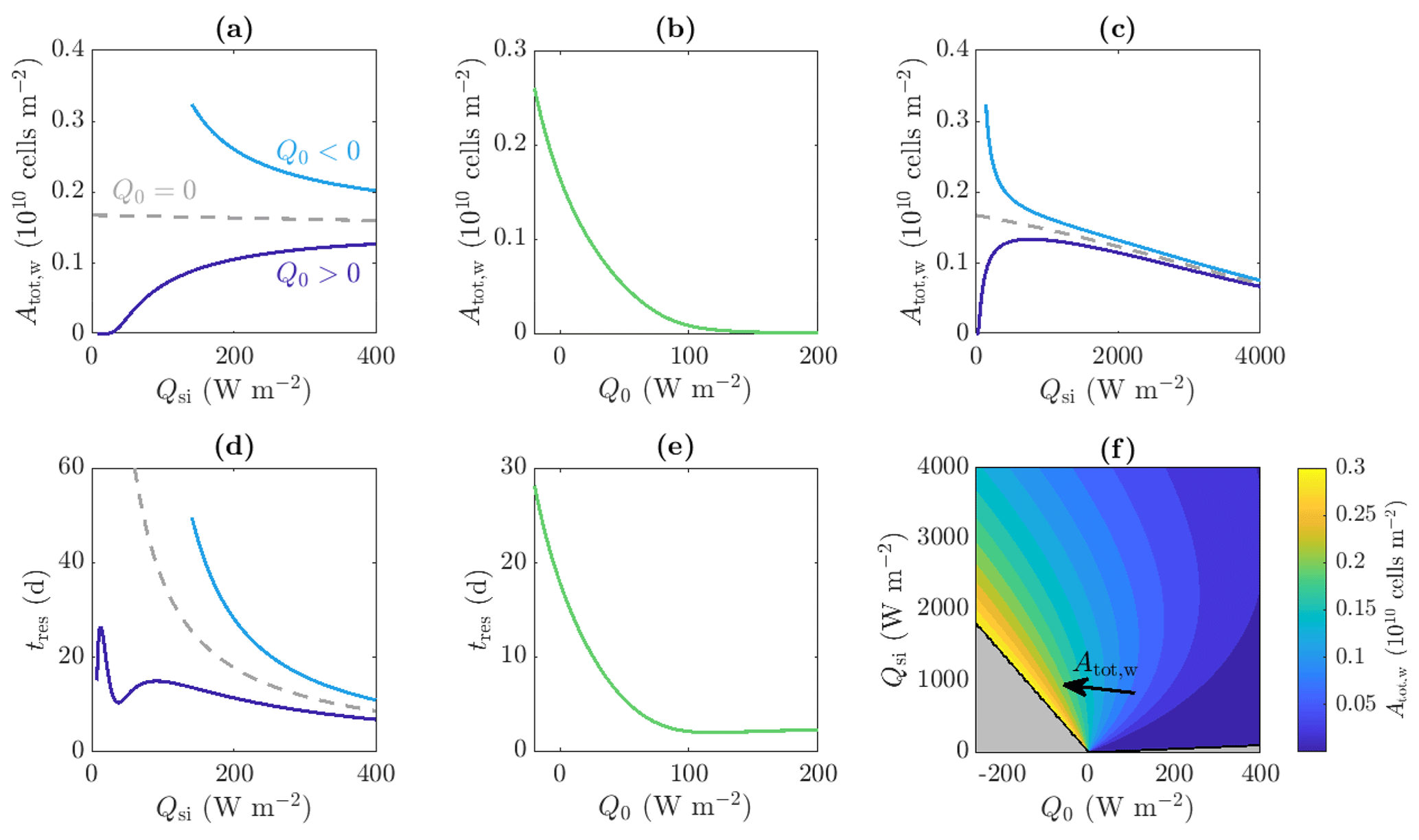
Figure 9 Dependence of (a, b, c, f) total amount of microbes in the water A_tot,w and (d, e) approximate residence time of the microbes t_res on the incoming shortwave radiation Q_si and other surface radiation Q₀. Panels (a), (c), and (d) show the solutions for Q₀=20 W m⁻² (dark blue line), $Q_{\mathrm{0}}=-\mathrm{20}$ W m⁻² (light blue line), and Q₀=0 W m⁻² (grey dashed line), respectively. Panels (b) and (e) show solutions with Q_si=200 W m⁻². Panel (c) is an extension of panel (a) to larger Q_si values. Panel (f) shows contours of A_tot,w in the region for which steadily melting states with both internal and surface melting are possible. The contour spacing is 0.02×10¹⁰ cells m⁻². The regions for which there is no surface melting and no internal melting are also shown (grey, see Fig. 4). The other parameter values are those shown in Table 1.

However, when Q₀<0, the total number of microbes A_tot,w decreases monotonically with increasing Q_si (compared to increasing when Q₀>0). The reason for this relates back to Fig. 4. As previously discussed, when Q₀<0, the melting depth Z_m decreases as Q_si increases because surface lowering increases at a faster rate than internal melting. Therefore, the region in which microbes can grow gets smaller, with the microbe distribution shifting upwards, as shown in Fig. 8a.

Figure 9b also shows how A_tot,w depends on the other surface radiation Q₀, which is a combination of net longwave radiation and turbulent heat fluxes, for a fixed value of shortwave radiation Q_si. We see that A_tot,w is a decreasing function of Q₀. This is because increasing Q₀ increases the surface melting without affecting the internal melting or microbial growth. Hence, the surface runoff increases without microbial growth increasing to compensate. When Q₀ gets large enough, there is no time for any microbial growth before the microbes get removed in runoff, so the microbial abundance remains close to the small background value A_∞.

The combined effect of Q_si and Q₀ on A_tot,w is shown in the contour plot in Fig. 9f. In addition to the behaviour captured by Fig. 9a–c, this shows how increasing Q₀ to more positive values causes the maximum of the blue A_tot,w against Q_si curve in Fig. 9c to decrease and move to a higher value of Q_si. As discussed, the total number of microbes A_tot,w is determined by a balance between the microbial growth in the interior and removal of microbes at the surface in runoff, with the position of the maximum being controlled by the point past which increasing Q_si further no longer increases the microbial growth significantly. When Q₀ is more positive, this point is delayed to larger Q_si because the size of the region in which microbial growth is possible, Z_m, takes longer to tend to its maximum value (see Fig. 4). Hence, for more positive Q₀, Qsi must get larger before A_tot,w starts decreasing with Q_si.

Importantly, the key result from Fig. 9f is that the total number of microbes in the water is largest when Q₀ is negative and Q_si is just large enough to allow surface melting, which are the conditions under which weathering crust growth is most favoured.

3.3.4 Residence times

Another quantity of interest is the residence time of the microbes – that is, how long the microbes remain in the weathering crust before being removed in runoff. This is of interest because it affects the carbon fluxes from the ice sheet – in particular whether or not the ice sheet is a net source or sink of CO₂. Cook et al. (2012) showed the Greenland ice sheet to be in a stable state of autotrophy (net removal of CO₂ from the atmosphere) due to the presence of cryoconite and surface algae, with increased warming leading to increased biomass and carbon fixation. However, they warned that too much warming could lead to the removal of microbes in runoff, reducing the removal of CO₂ from the atmosphere.

In our steadily melting model, we approximate the average residence time by

$$\begin{array}{}\text{(49)}& t_{\mathrm{res}}={\displaystyle \frac{A_{\mathrm{tot},\mathrm{w}}}{q}},\end{array}$$

where

$$\begin{array}{}\text{(50)}& q=-\dot{h}\mathit{\varphi }{A}_{\mathrm{w}}{|}_{Z=\mathrm{0}},\end{array}$$

is the microbial runoff rate at the surface. Equation (49) for t_res is the ratio between the amount of microbes in the water of the weathering crust and the rate at which the microbes are removed from the weathering crust. Therefore, we can think of t_res as being the average amount of time it would take to remove all the microbes from the weathering crust water. We can also interpret this as the average amount of time each microbe spends in the weathering crust, i.e. the residence time. Figure 9d shows the dependence of t_res on the incoming shortwave radiation Q_si. This is shown for positive (dark blue line) and negative (light blue line) values of Q₀. As with the total number of microbes A_tot,w, the observed behaviour is quite different depending on the sign of Q₀.

When Q₀>0, the global behaviour (ignoring the local minimum in Fig. 9d which we will discuss shortly) is that as Q_si increases, t_res initially increases then decreases again, for the same reasons as those just discussed around A_tot,w: as Q_si initially increases, the microbial growth rate increases so there are more microbes in the water, and these have to wait longer until they can be removed. Once Q_si is large enough to no longer be a limiting factor, the removal of microbes at the surface starts to dominate. This agrees with the previously discussed behaviour expected by Cook et al. (2012): increased warming leads to increased biomass (and residence times) until the microbes get removed by runoff. The local minimum observed in Fig. 9d occurs because the microbial abundance in the ice is small, $A_{\mathrm{i}}/A_{max}=A_{\mathrm{\infty }}/A_{max}=\mathrm{0.01}$. As Q_si increases, the microbial abundance A_w initially does not increase very much from A_∞ (seen from the flat section in Fig. 9a for small Q_si). When significant microbial growth does begin, growth first occurs at the surface, with the surface microbial abundance becoming quite large before the region of significant growth spreads downwards. When near-surface growth dominates, the microbial runoff rate q (which depends on the surface value of the microbial abundance) grows much more rapidly with Q_si than the total number of microbes A_tot,w because the microbial abundance is only growing significantly near the surface. Hence, the residence time t_res decreases. Once significant microbial growth begins spreading into the interior, A_tot,w grows more quickly than q, so t_res increases again.

However, when Q₀<0, t_res decreases monotonically with increasing Q_si (as does A_tot,w). The residence time decreases for the same reason that it decreases for large Q_si when Q₀>0 – increasing Q_si increases the surface lowering but does not increase the growth rate because radiation is high enough that it is no longer limiting. The non-monotonic behaviour for smaller Q_si is missed because Q_si cannot take such small values when Q₀<0, otherwise surface melting, and hence steadily melting states, would not be possible (see Fig. 4 and surrounding discussion in Sect. 2.3).

Figure 9e also shows that the approximate residence time t_res is a decreasing function of Q₀ for a fixed value of Q_si. This is for the same reasons (already discussed) that A_tot,w is a decreasing function of Q₀ for a fixed value of Q_si.

3.3.5 Summary

Our steadily melting state model has shown that microbial abundance in the weathering crust generally decreases with depth, as expected by Cook et al. (2016) and observed by Christner et al. (2018). This is because the radiation – which the microbes need to grow – decreases with depth. We have seen that significant microbial growth often only occurs in a top portion of the weathering crust, with the size of this region being controlled by microbial growth and nutrient parameters.

Furthermore, we have seen that the radiative forcings Q_si and Q₀ have a significant impact on the total number of microbes in the weathering crust and their residence time. This impact is via the balance between internal radiation (which favours growth of microbes and the weathering crust) and surface radiation (which increases surface melting and removal of microbes via runoff). In general, increasing internal radiation at a greater rate than surface radiation leads to an increase in the number of microbes and their residence time. In line with this, we observe different behaviour depending on the size of the shortwave radiation Q_si and the sign of the combined longwave radiation and turbulent heat fluxes Q₀, suggesting that the behaviour of the microbial population varies during the changeable conditions that lead to the formation and removal of the weathering crust. Recall that Q_si must be large enough for weathering crust formation to occur and that Q₀>0 favours removal (Muller and Keeler, 1969).

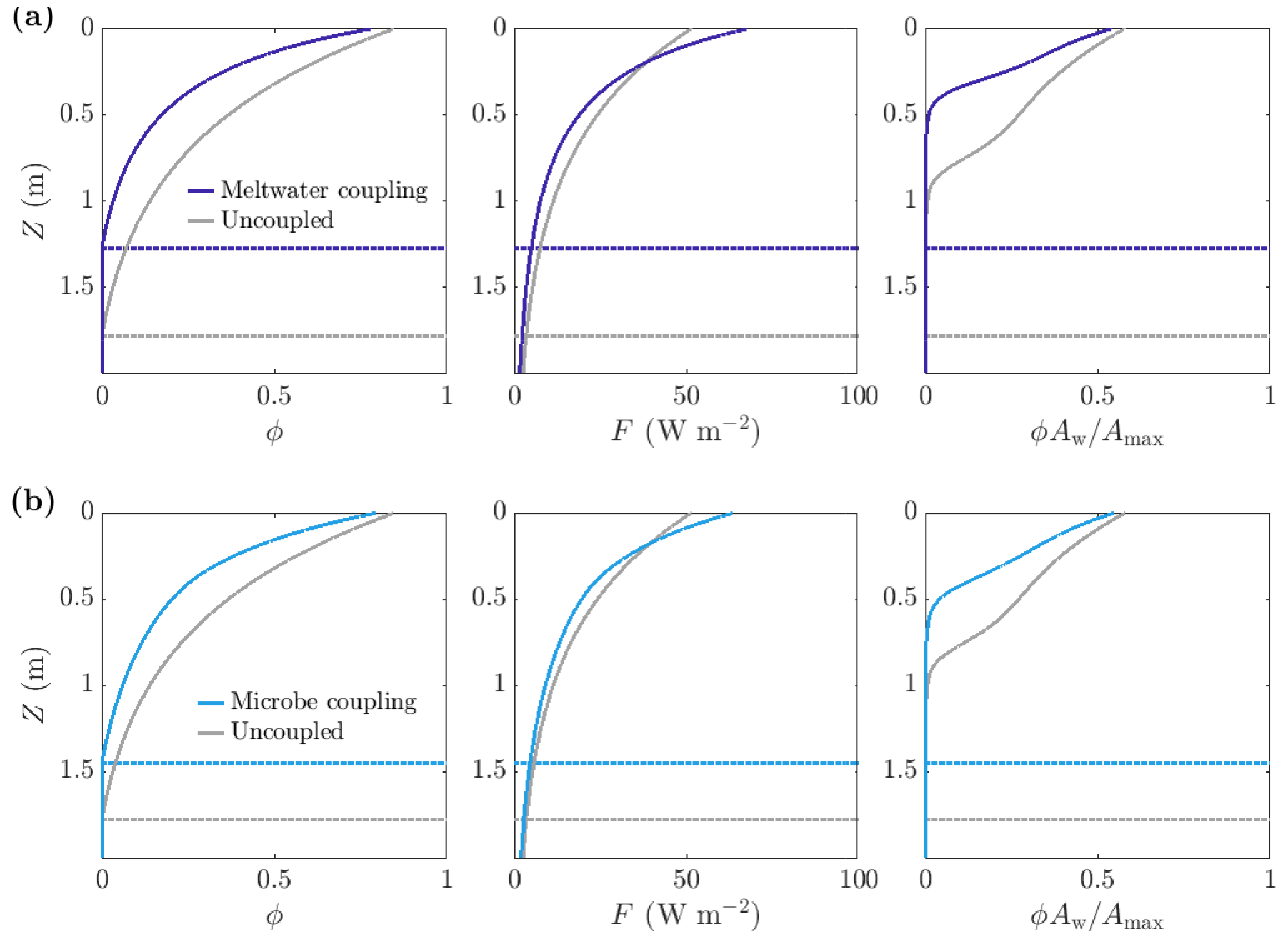
Figure 10 Comparison of steadily melting solutions with (dark and light blue) and without (grey) albedo feedbacks. Panel (a) shows meltwater coupling, where $\mathit{\alpha }={\mathit{\alpha }}_{\mathrm{0}}(\mathrm{1}+\mathrm{3}\mathit{\varphi })$, so that the absorption increases with water content. The albedo in the coupled case is 0.47, compared to 0.6 in the uncoupled case. Panel (b) shows microbe coupling, where $\mathit{\alpha }={\mathit{\alpha }}_{\mathrm{0}}(\mathrm{1}+\mathrm{3}\mathit{\varphi }(A_{\mathrm{w}}-A_{\mathrm{\infty }}\left)\right)$, so that the absorption increases with the bulk microbial abundance. The albedo in the coupled case is 0.51. The dotted lines show the melting depth Z_m. The parameter values are those shown in Table 1.

4 Feedbacks between microbial growth, albedo, and melting

The weathering crust and the microbes within it give rise to some potential albedo feedbacks that can lead to amplified reductions in albedo and increases in melting. Here we will discuss the melt–albedo feedback (e.g. Box et al., 2012) and the microbe–albedo feedback (e.g. Tedstone et al., 2020; McCutcheon et al., 2021) and explore the ability of our model to capture and quantify these feedbacks. We first briefly outline the potential feedbacks.

As the surface of an ice sheet melts, the surface transitions from snow covered to bare ice to having meltwater on the surface. The change in surface type from snow-covered to water-covered surfaces leads to a reduction in the albedo. This in turn means that more radiation is absorbed, so more melting occurs, reducing the albedo further. The result is a positive feedback: the melt–albedo feedback (e.g. Box et al., 2012).

The surface of ice sheets can also be made darker by biological factors, especially glacier ice algae and cryoconite (Hotaling et al., 2021), with glacier ice algae thought to be a key contributor to the darkening of the Greenland ice sheet (Benning et al., 2014). There is thought to be a potential positive feedback between ice algae and meltwater, whereby the presence of algae on the ice-sheet surface lowers the albedo, increasing melting, which releases nutrients that had been frozen in the ice, enabling more algal growth (e.g. Tedstone et al., 2020; McCutcheon et al., 2021). The darkening effect is particularly strong for surface ice algae because the algae have a special dark pigment to protect them from high levels of UV and photosynthetically active radiation (Williamson et al., 2019, 2020). However, a similar, but weaker, feedback can be expected for microbes in the weathering crust. Furthermore, the framework we provide here for studying microbe–albedo feedback in the weathering crust can be easily adapted to ice algae.

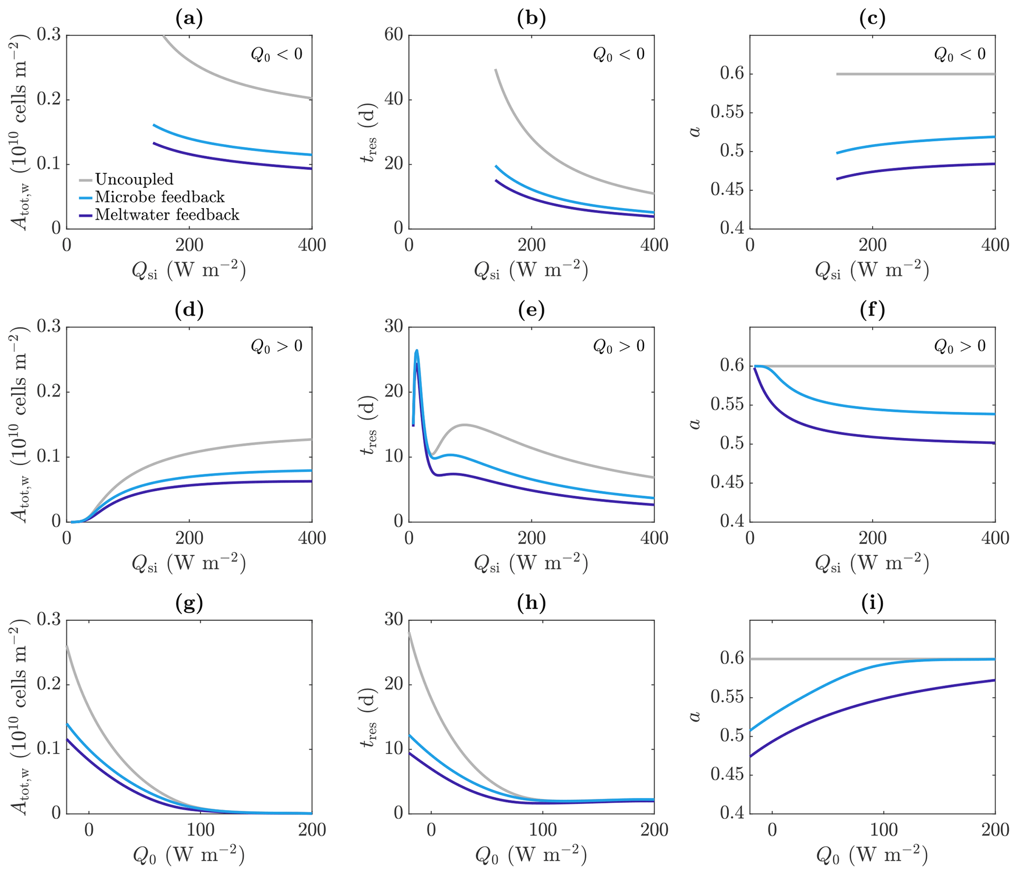
Figure 11 Dependence of (a, d, g) total amount of microbes in the water A_tot,w, (b, e, h) approximate residence time of the microbes t_res, and (c, f, i) albedo a on the incoming shortwave radiation Q_si (a–f) and other surface radiation Q₀ (e–g), in the uncoupled (grey), meltwater coupling (dark blue), and microbe coupling (light blue) cases. The value of Q₀ is −20 W m⁻² (negative) in (a)–(c) and 20 W m⁻² (positive) in (d)–(f). The value of Q_si is 200 W m⁻² in (g)–(i). The other parameter values are those shown in Table 1.

4.1 Model

To introduce the melt–albedo and microbe–albedo feedbacks into our steadily melting model, we make the absorption coefficient α a linearly increasing function of either the porosity ϕ or the bulk microbial abundance $A_{\mathrm{bulk}}=\mathit{\varphi }{A}_{\mathrm{w}}+(\mathrm{1}-\mathit{\varphi })A_{\mathrm{i}}$. This captures the fact that more shortwave radiation is absorbed when there is more water (compared to ice) or when there are more microbes. The albedo a is then calculated as an output of the model from the additional boundary condition (22), as discussed in Sect. 2. The absorption coefficient functions we chose are

$$\begin{array}{}\text{(51)}& \mathit{\alpha }={\mathit{\alpha }}_{\mathrm{0}}(\mathrm{1}+\mathrm{3}\mathit{\varphi }),\end{array}$$

to capture the melt–albedo feedback and

$$\begin{array}{}\text{(52)}& \mathit{\alpha }={\mathit{\alpha }}_{\mathrm{0}}(\mathrm{1}+\mathrm{3}(A_{\mathrm{bulk}}-A_{\mathrm{\infty }}\left)\right)={\mathit{\alpha }}_{\mathrm{0}}(\mathrm{1}+\mathrm{3}\mathit{\varphi }(A_{\mathrm{w}}-A_{\mathrm{\infty }}\left)\right),\end{array}$$

to capture the microbe–albedo feedback, where we have used that A_i=A_∞ in our steadily melting setup. Here, α₀ is the absorption coefficient of pure ice containing the small background abundance of microbes A_∞. The specific forms of Eqs. (51) and (52) have been chosen as a simple way to include the feedbacks in our model. The value 3 we have chosen in Eqs. (51) and (52) is arbitrary and using other positive values leads to qualitatively the same results. We are not aware of any literature detailing the dependence of the absorption coefficient on porosity and microbial abundance.

4.2 Results

By making the absorption coefficient a function of the porosity ϕ and/or the microbial abundance A_w, the steadily melting weathering crust problem can no longer be solved analytically. Furthermore, a dependence on A_w fully couples the microbe and nutrient problem to the weathering crust problem, meaning that we can no longer solve the weathering crust problem on its own first. Therefore, we must solve the full problem numerically. It is still possible to find the solution in Z>Z_m analytically, whereas the solution in Z<Z_m is found numerically using the boundary value problem solver bvp4c in MATLAB. Our code is made available at https://doi.org/10.5281/zenodo.7199159 (Woods, 2022).

As expected, making the absorption of shortwave radiation increase with water content or microbial abundance causes a reduction in albedo in our model (Fig. 11c). We find that including the meltwater coupling (Eq. 51) reduces the albedo to 0.47 compared to 0.6 in the uncoupled case with α=α₀. Similarly, the microbe coupling (Eq. 52) reduces the albedo of the steadily melting solution to 0.51 from 0.6.

Figure 10 shows a comparison between the porosity, internal radiation, and microbial abundance distributions in the coupled and uncoupled cases. The effects of including meltwater coupling and microbe coupling are similar. In both cases, more radiation is absorbed by the ice than in the uncoupled case (seen in the reduction in albedo). However, the internal radiation does not increase everywhere – it is higher than the uncoupled case near the surface but lower at depth. This is because there is more water and more microbial biomass near the surface, so absorption of radiation is greatest near the surface, which in turn means that there is less radiation left to penetrate deeper into the ice.

The overall effect of including the coupling is to decrease the size of the weathering crust (decrease Z_m), lower the porosity, and reduce the total amount of microbes (Fig. 10). This might seem counter-intuitive; the feedbacks previously discussed would suggest that making the absorption depend on water content or microbial abundance would lead to an increase in water content and microbial abundance since more water and microbes leads to greater absorption, resulting in even more melting and microbial growth. However, we are observing the previously discussed removal of microbes in runoff proposed by Cook et al. (2012). The increase in absorption has led to an increase in surface melting, lowering, and runoff, with enhanced removal of microbes in runoff dominating any increase in microbial growth. Therefore, including the coupling leads to an upward translation of the microbial abundance distribution, as we saw in Sect. 3.3.2.

Figure 11 reproduces the plots of the total number of microbes in the water A_tot,w and residence time t_res as a function of Q_si from Fig. 9; this time it shows the results for meltwater coupling, microbe coupling, and the uncoupled case from Fig. 9 (grey). The variation with Q_si for Q₀<0 (top row) and Q₀>0 (middle row) is shown, as well as the variation with Q₀ (bottom row). These show that including the meltwater or microbe coupling reduces the total number of microbes and reduces their residence time, with the main effect when Q₀>0 being to reduce the second local maximum. This is because the region of significant algal growth is smaller with coupling (Fig. 10), so the increase in t_res from the local minimum to the second local maximum, which corresponds to the spread of the significant microbial growth region deeper into the ice (discussed around Fig. 9), is reduced.

Note that Fig. 11 shows that the total number of microbes, residence time and albedo are all lower with meltwater coupling than microbe coupling, but this should not be read into too much. The forms of the absorption coefficient functions (51) and (52) are illustrative only and could easily be modified such that the microbe coupling has a larger effect (e.g. by replacing 3 in Eq. (52) with a larger value). The main point to take away from this investigation is that including coupling between meltwater, microbes, and radiation absorption can lead to a reduction in albedo but also a reduction in the size of the weathering crust and the total microbial abundance within the weathering crust aquifer. Due to excluding surface ice algae from our model, we are unable to draw any conclusions about the total microbial abundance of the whole system, comprised of both microbes in the weathering crust aquifer and algae on the ice surface.

5 Discussion and conclusion

We have presented a mathematical model for the weathering crust and the microbes within it, as well as a nutrient for the microbes. We have focussed on one-dimensional steadily melting solutions, where the internal and surface melt rates balance to produce a weathering crust of a steady size. We have assumed that all surface meltwater runs off, removing any microbes or nutrients that were in the water. In reality, the lateral flow of meltwater across the ice-sheet surface and through the weathering crust is important for the transport of nutrients and microbes across the ice (e.g. Stibal et al., 2012), but our one-dimensional model is unable to capture this.

We have made a number of simplifications in order to produce a reduced problem from which we can gain informative insights. One simplification of reality is our treatment of the microbes and their nutrients. We have assumed that there is a single type of phototrophic microbe and a single representative nutrient for the microbe. In reality, the weathering crust contains a range of different microbes: primary producers (e.g. algae and filamentous cyanobacteria), which use solar radiation as their energy source, and heterotrophs, which use autochthonous organic carbon produced by the primary producers as their energy source (Stibal et al., 2012). Our model could be thought of as describing a single representative type of primary producer, which requires both solar radiation and nutrients for growth. Alternatively, it could be interpreted as modelling (crudely) the combined influence of all microbes. Clearly there are more complex interactions that could be added at the expense of introducing further parameters and potentially losing interpretability.

Similarly, the reality is that microbes require multiple nutrients to survive and grow, namely carbon (C), nitrogen (N), phosphorous (P), and a variety of micronutrients. The representative nutrient in our model can be interpreted as whichever of the three macronutrients (C, N, or P) is limiting. In the case of glacier ice algae and cryoconite microbial communities, P is usually the limiting nutrient (McCutcheon et al., 2021; Stibal and Tranter, 2007; Bagshaw et al., 2013).

Our model has given insight into the porosity and microbe distributions in the weathering crust. Our model shows that the porosity decreases non-linearly with depth, in agreement with previous observations (Schuster, 2001; Cooper et al., 2018) and modelling (Schuster, 2001). However, the surface values of porosity in our model are larger than observed by Schuster (2001) and Cooper et al. (2018) (∼0.85 compared to ∼0.65). This could be due to our assumption that the entire crust is saturated, neglecting the observed unsaturated surface layer. The presence of near-surface water in our model leads to increased absorption and melting compared to if the near-surface was unsaturated. Furthermore, we would expect the crust to disintegrate once the porosity gets above a certain limit, but this is not included in our model. We have also found the microbial abundance in the weathering crust generally decreases with depth. This agrees with the expectation of Cook et al. (2016) and the observations of Christner et al. (2018). Since radiation decreases with depth, it is expected that there will be more primary producers (with protective pigments) near the surface and more heterotrophs (which are less adapted to light) deeper down (Cook et al., 2016). The decrease in radiation with depth also leads to a decrease in porosity and melting with depth.

Furthermore, we have observed that the climate forcing (represented by the shortwave radiation Q_si and combined longwave radiation and turbulent heat fluxes Q₀ in our model) has a clear impact on the size of the weathering crust and the residence time and abundance of microbes in the weathering crust. Our model shows that it is the balance between internally absorbed radiation and surface forcings that controls these quantities. The relationship is complex, but, in general, increasing the surface forcings relative to internal radiation (for example, increasing the turbulent heat fluxes and longwave radiation Q₀) causes the size of the weathering crust, the residence time, and the total number of microbes in the crust to all decrease. This is due to enhanced surface melting and runoff causing removal of the weathering crust and the microbes within it. This is in line with the observation that warm, windy, overcast conditions (high turbulent heat fluxes) favour weathering crust removal (Muller and Keeler, 1969), as well as the suggestion that excessive warming could lead to a removal of microbes in runoff, threatening the Greenland ice sheet's state of autotrophy (net removal of CO₂) (Cook et al., 2012).

Our model also allows for the investigation of positive feedbacks. We have explored melt–albedo and microbe–albedo feedbacks by making the absorption of shortwave radiation a function of the water and microbe content of the weathering crust, respectively. These feedbacks lead to enhanced melting of the ice-sheet surface. Our model suggests that both feedbacks act to reduce the weathering crust size and number of microbes in the weathering crust aquifer, as well as their residence times. This is due to enhanced melting leading to an increased runoff rate, so more microbes get removed from the surface. Hence, these feedbacks are self-limiting – the reduction in albedo cannot keep going unlimited because the increased melting will lead to the removal of the microbes and meltwater that cause the albedo reduction.

However, we caution that we have focussed on microbes that live within the weathering crust aquifer (transported by meltwater), and have ignored the glacier ice algae that live on the surface of the weathering crust (affixed to the ice). An area for future work is to extend our model to include a population of surface algae that can persist in the presence of meltwater runoff, necessitating a removal of our assumption that all microbes get washed away in runoff. This would enable more to be said about the total system microbial abundance of the weathering crust, including that stored on the surface. Moreover, the surface algae provide a major contribution to the albedo via the algal blooms that occur on the south-western Greenland ice sheet. Extending our modified surface ice algae model to higher dimensions would enable an investigation of the spatio-temporal dynamics of algal blooms and their impact on albedo.

In a similar vein, our model could be used to investigate the temporal dynamics of the weathering crust across a full melt season at locations in the field, such as in the “dark zone” on the south-western Greenland ice sheet. This would allow us to better understand the changeable behaviour of the weathering crust in response to variable weather conditions. Another benefit would be to provide a physical approach to developing a bare-ice albedo scheme. The bare-ice albedo schemes used in major climate models are often very simple and do not compare well with in situ observations (e.g. Fettweis et al., 2017), so alternative approaches are desirable.

In conclusion, we have shown that a mathematical model can be used to capture and explore key characteristics and behaviours of the weathering crust and the microbes within it. In particular, even with a number of simplifications, it shows that the response of the weathering crust and its microbial community to changes in atmospheric forcing is complex, and can lead to both increases and decreases in microbial abundance. We acknowledge that the model has crudely approximated many aspects of the dynamics but hope that this study can provide a framework into which more detailed biogeochemistry and physics can be incorporated in the future.