Geothermal heat flux is the dominant source of uncertainty in englacial-temperature-based dating of ice rise formation

Ice rises are areas of locally grounded, slow-moving ice adjacent to floating ice shelves. Temperature profiles measured through ice rises contain information regarding changes to their dynamic evolution and external forcings, such as past surface temperatures, past accumulation rates and geothermal heat flux. While previous work has used borehole temperature–depth measurements to infer one or two such parameters, there has been no systematic investigation of parameter sensitivity to the interplay of multiple external forcings and dynamic changes. A one-dimensional vertical heat flow forward model developed here examines how changing forcings affect temperature profiles. Further, using both synthetic data and previous measurements from the Crary Ice Rise in Antarctica, we use our model in a Markov chain Monte Carlo inversion to demonstrate that this method has potential as a useful dating technique that can be implemented at ice rises across Antarctica. However, we also highlight the non-uniqueness of previous ice rise formation dating based on temperature profiles, showing that using nominal values for forcing parameters, without taking into account their realistic uncertainties, can lead to underestimation of dating uncertainty. In particular, geothermal heat flux represents the dominant source of uncertainty in ice rise age estimation. For instance, in Crary Ice Rise higher heat flux values (i.e. about 90 mW m⁻²) yield grounding timing of 1400 ± 800 years, whereas lower heat flux of around 60 mW m⁻² implies earlier ice rise formation and lower uncertainties in the ice rise age estimations (500 ± 250 years). We discuss the utility of this method in choosing future ice drilling sites and conclude that integrating this technique with other indirect dating methods can provide useful constraints on past forcings and changing boundary conditions from in situ temperature–depth measurements.

1 Introduction

Present-day englacial temperatures are the product of the millennial-scale histories of ice flow and thermal boundary conditions experienced by an ice sheet (Robin, 1955). Temperature measurements from boreholes drilled through ice sheets have been widely used to extract important palaeoclimatic archives, such as surface temperature and accumulation history, as well as information about the conditions at the base of an ice sheet (i.e. glacial thermal regime and geothermal heat flux), both in Antarctica and Greenland (see Dahl-Jensen and Johnsen, 1986; Dahl-Jensen et al., 1998; Engelhardt, 2004a; Orsi et al., 2012; Cuffey et al., 2016). In Antarctica, the ice sheet contains ice rises – regions of slow-flowing, locally elevated grounded ice embedded within or adjacent to fast-flowing, floating ice shelves; one way they form is through an ice-shelf grounding on marine bed (e.g. Martin and Sanderson, 1980; Matsuoka et al., 2015; Wearing and Kingslake, 2020). This shift in boundary condition at the base of an ice sheet results in a transient evolution of the temperature–depth profile within an ice rise (MacAyeal and Thomas, 1980; Bindschadler et al., 1990). Therefore, due to their proximity to the marine ice-sheet periphery and negligible horizontal flow, ice rises can retain an imprint of past grounding line migration on millennial timescales, a record that is otherwise largely inaccessible beneath the ice sheet or its fringing ice shelves (e.g. Conway et al., 1999; Matsuoka et al., 2015; Kingslake et al., 2018; Neuhaus et al., 2021).

Past work used temperature–depth measurements within ice rises in Antarctica to estimate the timing of ice-shelf grounding. For instance, Bindschadler et al. (1990) developed an advection–diffusion thermal model of Crary Ice Rise, West Antarctica (Fig. 1). The model calculated the initial steady-state ice-shelf temperature profile from the specified set of parameters, including ice thickness, surface temperatures and accumulation rates. The steady-state ice-shelf profile was perturbed using thermal properties of the bed (geothermal heat flux, diffusivity and conductivity of the bedrock) and a specified vertical ice velocity function to calculate transient thermal evolution after ice-shelf grounding. The modelled temperature profiles were then compared to in situ borehole measurements at Crary Ice Rise, and minimising the mismatch between the measured and synthetic profiles yielded the best age estimate of the ice rise in its thickest part to be 1100 years. Recent work by Neuhaus et al. (2021) built upon the model of Bindschadler et al. (1990) to evaluate the timing of grounding at three sites in the Ross Sea sector of Antarctica, where previous measurements showed anomalously high basal temperature gradients (Engelhardt, 2004a). These results largely corroborate hypotheses of late Holocene re-advance in the region (Kingslake et al., 2018) and associated grounding at these sites between 1100 and 500 years ago (Neuhaus et al., 2021).

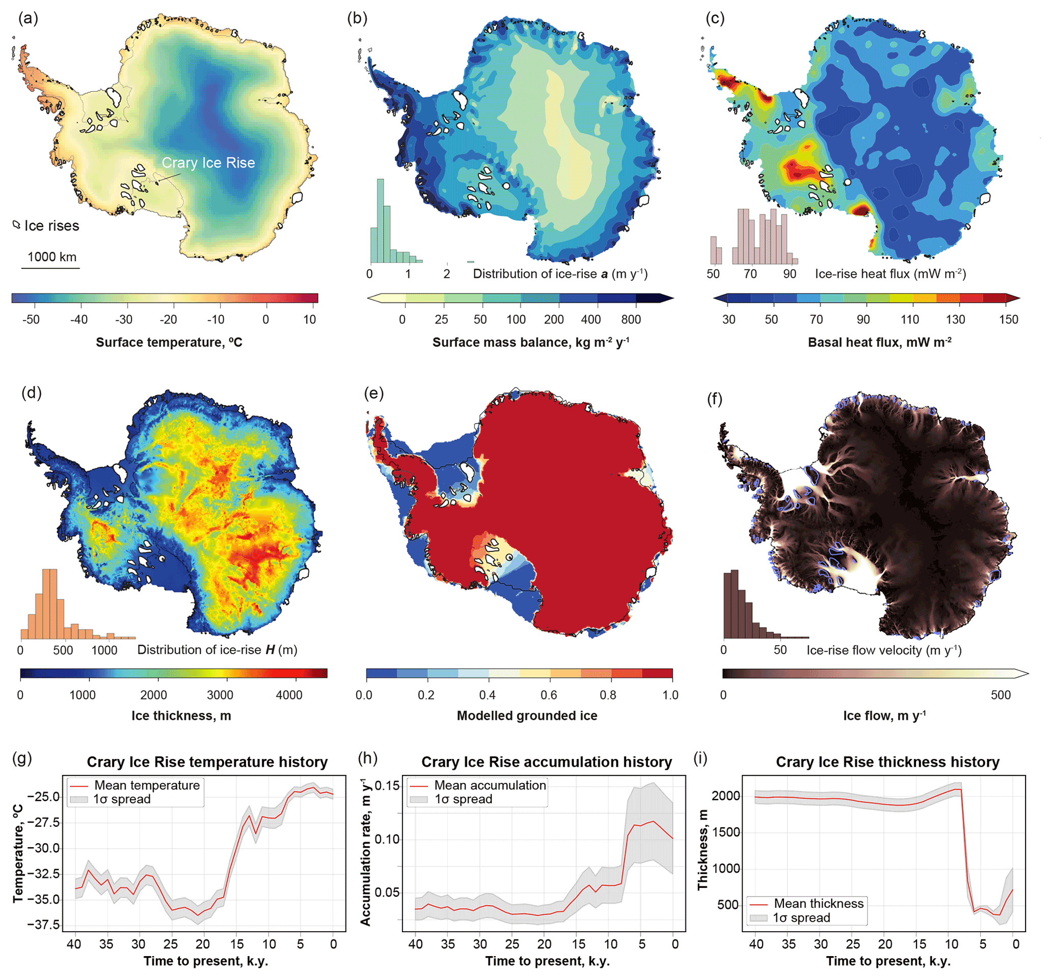
Figure 1 Present-day distribution of key parameters affecting temperature–depth profiles in Antarctica. (a) ERA-Interim annual mean surface temperatures (Albrecht et al., 2020a). White areas in (a)–(e) indicate locations of ice rises from an Antarctic-wide inventory presented in Matsuoka et al. (2015). (b) Mean surface mass balance (that is, the difference between accumulation and ablation at the ice-sheet surface) for the period 1979–2015 (Agosta et al., 2019) and distribution of approximate accumulation rates extracted for all ice rise locations. (c) Basal geothermal heat flux reconstructed from magnetic data (Martos et al., 2017) and distribution of heat flux below ice rises. (d) Ice thickness and ice rise thickness distribution (Fretwell et al., 2013). (e) Ensemble-score-weighted grounded mask for the present-day ice sheet, reflecting possible histories of grounding line migration since deglaciation (Albrecht et al., 2020b). Red colour indicates grounded areas which are covered by grounded ice in all simulations. Blue colour indicates areas which are covered by few simulations with low scores. (f) Ice-flow surface velocity (Arthern et al., 2015). The grounding line and coastlines are shown in black. Arrow on (a) shows the location of Crary Ice Rise, where previously the timing of grounding was inferred using borehole temperature measurements (Bindschadler et al., 1990). (g–i) Forty-million-year histories of surface temperature, accumulation and thickness in the vicinity (i.e. within about 200 km) of Crary Ice Rise obtained from large-scale Parallel Ice Sheet Model (PISM) simulations (Kingslake et al., 2018; Albrecht et al., 2020a, b).

Thus, the methods used in these studies have potential if future boreholes are drilled at Antarctic ice rises in locations suspected of undergoing significant dynamic changes. Yet, the uncertainties inherent in these approaches must be carefully assessed to target drilling, maximise the utility of borehole drilling and increase the accuracy of ice dynamics inferences and palaeoclimatic inferences. Previous work has included sensitivity tests where some predefined variables, such as accumulation, ice thickening and melt rate, were assigned several different values to examine how they affected the final temperature profile and their relation to inferred timing of grounding (Bindschadler et al., 1990; Neuhaus et al., 2021). Yet, there is a lack of systematic investigations of temperature profile sensitivity to the cumulative effects of multiple external forcings and dynamic changes, particularly given that some parameters (e.g. geothermal heat flux) have considerable uncertainties (e.g. Fudge et al., 2019). In addition, time-variable parameters, such as ice thickness, accumulation and surface temperature may significantly increase the dimensionality of the problem, solutions to which need optimised inversion methods, as opposed to exhaustive global search algorithms where highly dimensional inversion tasks become computationally unfeasible (Mosegaard and Tarantola, 1995).

Here we use forward modelling to investigate how the interplay between forcings and parameters (i.e. surface temperature, accumulation rate, heat flux and thickness history) affects the englacial temperatures. Using previous measurements from the Crary Ice Rise, West Antarctica (Fig. 1), we also implement a Markov chain Monte Carlo inversion to explore the contributions of multiple uncertainties to the inferred timing of ice rise formation.

2 Methods

In this section we outline the numerical forward model and inversion method. The forward model builds upon and extends the models used by Alley and Koci (1990), Orsi et al. (2012), and Neuhaus et al. (2021). The inversion method is similar to that previously used to reconstruct past surface temperatures in Greenland and Antarctica (e.g. Dahl-Jensen et al., 1998, 1999). Extending previous work, we include the effects of different vertical velocity functions, we use an optimised set of some parameters (e.g. pressure melting/freezing point of ice/seawater), and we introduce temporal variability to ice thickness, surface temperature and accumulation rates, as well as multiple phases of grounding and ungrounding and corresponding changes to the boundary conditions.

2.1 Forward model

2.1.1 Model equations

We use the following form of the vertical diffusion–advection equation to simulate the time and depth evolution of temperature T:

$$\begin{array}{}\text{(1)}& {\displaystyle \frac{\partial T}{\partial t}}=\mathit{\alpha }{\displaystyle \frac{{\partial }^{\mathrm{2}}T}{\partial z}}-w{\displaystyle \frac{\partial T}{\partial z}},\end{array}$$

where t is time, z is height above the bed, w is vertical ice velocity (positive upwards) and α is thermal diffusivity.

$$\begin{array}{}\text{(2)}& \mathit{\alpha }={\displaystyle \frac{k}{\mathit{\rho }c}},\end{array}$$

where ρ is density, k is the thermal conductivity and c is the specific heat capacity. We assume that α is uniform and constant, and the internal heat production can be neglected due to insignificant horizontal ice flow (Dahl-Jensen et al., 1999), typically on the scale of metres per year (e.g. Matsuoka et al., 2015; Kingslake et al., 2016).

For sensitivity experiments, we implement three analytical approximations for vertical velocity w within grounded ice. The Dansgaard and Johnsen (1969) vertical flow approximation can be formulated as

$$\begin{array}{}\text{(3)}& {\displaystyle }w(z,z_k)=-w_{\mathrm{s}}\left(t\right){\displaystyle \frac{\mathrm{2}z-z_k}{\mathrm{2}H-z_k}}\text{ for }{z}_k\le z\le H,\text{(4)}& {\displaystyle }w(z,z_k)=-w_{\mathrm{s}}\left(t\right){\displaystyle \frac{z^{\mathrm{2}}}{(\mathrm{2}H-z_k)z_k}}\text{ for }\mathrm{0}\le z\le z_k,\end{array}$$

where w_s is time-varying vertical velocity at the surface, z=0 represents the ice–bedrock interface, H is the ice thickness and z_k is a free parameter (Martín and Gudmundsson, 2012). Lliboutry (1979) provides another commonly used approximation (Wearing and Kingslake, 2019; Fudge et al., 2019):

$$\begin{array}{}\text{(5)}& \begin{array}{rl}w(z,t)& =w_{\mathrm{s}}\left(t\right)\left[\mathrm{1}-{\displaystyle \frac{n+\mathrm{2}}{n+\mathrm{1}}}\left(\mathrm{1}-{\displaystyle \frac{z}{H\left(t\right)}}\right)\right.\\ & \left.+{\displaystyle \frac{\mathrm{1}}{n+\mathrm{1}}}{\left(\mathrm{1}-{\displaystyle \frac{z}{H\left(t\right)}}\right)}^{n+\mathrm{2}}\right],\end{array}\end{array}$$

where n is a rheological parameter (Glen's flow law exponent, n=3).

Finally, a simplified approximation where vertical velocity varies linearly with depth from zero at the base to a maximum value at the surface, following Bindschadler et al. (1990), was implemented for sensitivity experiments and estimation of associated uncertainties:

$$\begin{array}{}\text{(6)}& w(z,t)=w_{\mathrm{s}}\left(t\right){\displaystyle \frac{z}{H\left(t\right)}}.\end{array}$$

When time-varying ice thickness is introduced, the difference between accumulation and thickening rates determines the vertical velocity at the surface:

$$\begin{array}{}\text{(7)}& w_{\mathrm{s}}\left(t\right)=a\left(t\right)-{\displaystyle \frac{\partial H\left(t\right)}{\partial t}}.\end{array}$$

For temperature calculations within the underlying bedrock, no vertical advection is assumed (w=0), reducing Eq. (1) to only account for heat diffusion.

2.1.2 Spatiotemporal domain and boundary conditions

We define a one-dimensional spatial domain that extends vertically from the bedrock base to the ice surface. The vertical coordinate is z, which increases upwards, and z_b and z_s are the elevations of the ice base and ice surface, respectively. We implement a simple finite-difference scheme to solve Eq. (1). We discretise the spatial domain with a minimum of 50 nodes within the ice column and 50 nodes with fixed 10 m vertical spacing in the subjacent bedrock (Neuhaus et al., 2021). We used a time step of 1 year. In a scenario where ice thickness varies through time, vertical grid spacing in the ice column is adapted and temperature values are interpolated accordingly at each time step. The model can be run under two different assumptions about whether the ice column is a part of a grounded ice rise or a floating ice shelf.

In the ice-shelf scenario (Fig. 2a) boundary conditions at the ice surface are set by time-variable surface temperatures T(t) and accumulation rates a(t). The temperature at the top of the bedrock/base of ice column T(z=z_b) is forced to equal the freezing point of seawater (calculated as a function of ice thickness to account for its pressure dependence), and the temperature gradient in the bedrock is calculated based on the geothermal heat flux G (Millero, 1978; Determann and Gerdes, 1994). We assume that the rates of accumulation and basal melting balance the depth-uniform vertical velocity (Holland and Jenkins, 1999).

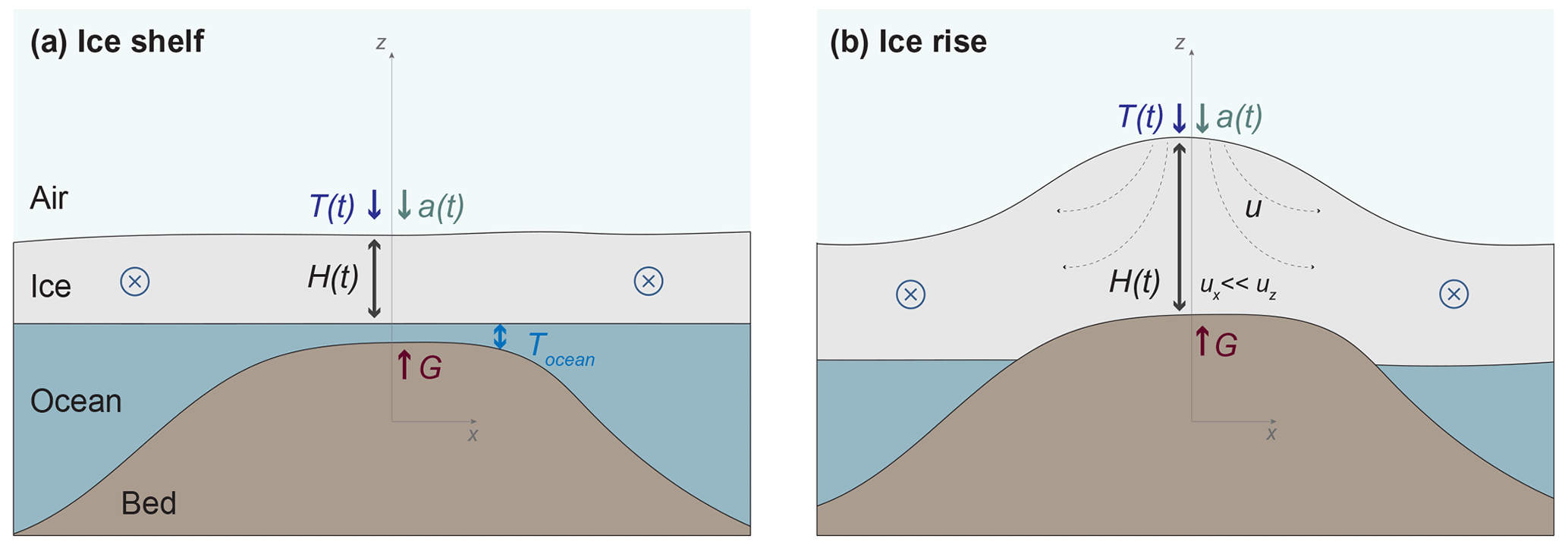
Figure 2 Geometry of the ice shelf and ice rise heat flow model. The simple one-dimensional vertical model is implemented along a stationary crest of hypothetical ice rise (z axis on the figure) and bedrock beneath it. T(t) and a(t) indicate surface temperature and accumulation forcings, respectively. G is geothermal heat flux, and u is ice-flow velocity (along the crest of ice rise, horizontal flow velocity u_x is negligibly small comparable to its vertical component u_z or w).

When modelling temperatures within a grounded ice sheet (i.e. an ice rise; see Fig. 2b), the boundary condition at the base of the ice column is set such that the vertical gradient in T corresponds to a diffusive heat flux (there is no advection because w(z_b)=0) that balances the geothermal heat flux G through the underlying bedrock. Thickness history H(t) and the vertical velocity function (Eqs. 3–6) within the ice rise are also used. The boundary conditions at the top of the ice column are prescribed based on the temperature and accumulation rate histories; prior values of parameters that dictate these boundary conditions are discussed further in Sect. 2.1.3.

2.1.3 Input parameters

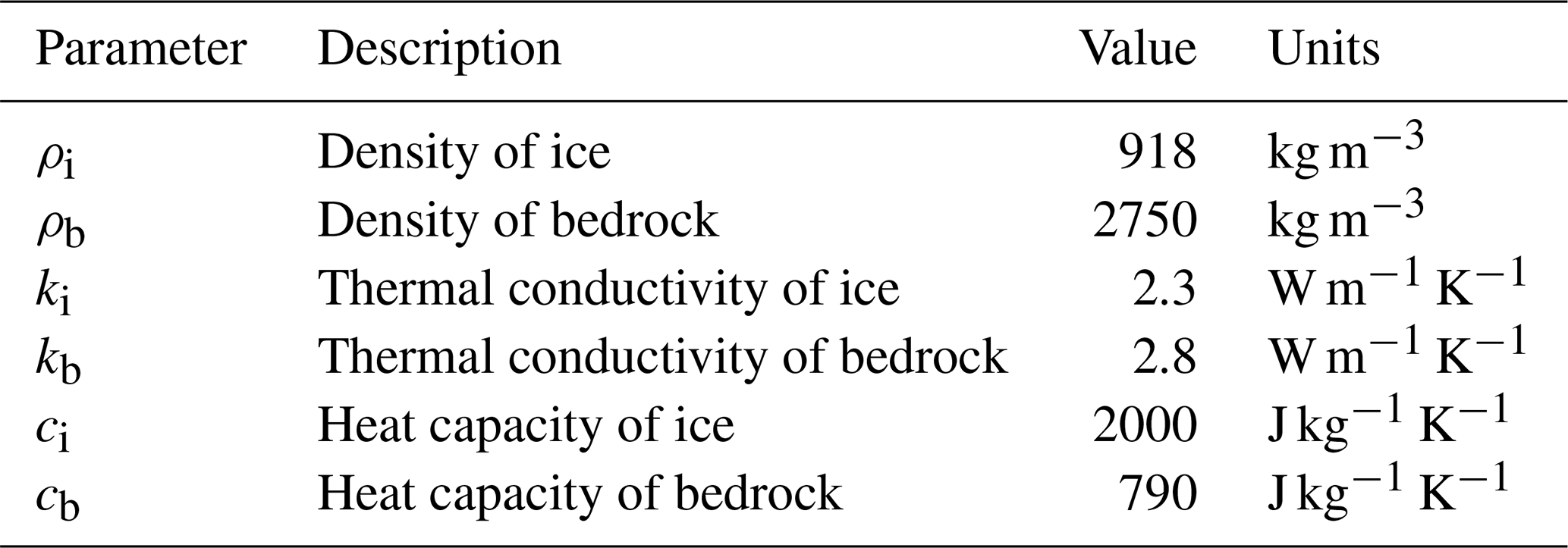
Parameters characterising the properties of ice and the bedrock are assumed to be constant (Table 1). Values of geothermal heat flux at specific locations are sampled from the Antarctic-wide heat flux data compilation derived from spectral analysis of airborne magnetic data (Martos et al., 2017). Surface temperature evolution, accumulation rate histories and ice-thickness histories are sampled from distributions provided by an ensemble of simulations using the Parallel Ice Sheet Model (PISM) (Fig. 1g–i; Kingslake et al., 2018; Albrecht et al., 2020a, b). PISM is a three-dimensional, thermomechanical ice-sheet model that solves a hybrid shallow approximation of Stokes flow. PISM produces continental-scale (16 km grid cell size), long-term (multi-millennia length) simulations of ice-sheet thickness. Associated with these fields are surface temperatures reconstructed from the West Antarctic Ice Sheet (WAIS) divide ice core (Cuffey et al., 2016), scaled by modelled ice-surface elevation and accumulation patterns simulated by the regional climate model RACMOv2.1 (Ligtenberg et al., 2013) and scaled by 2 % per degree of temperature change from present (Kingslake et al., 2018). Other specifications and parameters used for the chosen PISM model output, including mantle viscosity and flexural rigidity, are described in detail in Kingslake et al. (2018). Despite inherent uncertainties associated with large-scale numerical models, which have relatively coarse resolution compared to the length scales of ice rises, PISM outputs provide first-order estimates of prior information about the time-variable parameters (i.e. temperature, accumulation and ice thickness) at any specified location on the Antarctic Ice Sheet (AIS) (Fig. 1e–f).

Table 1 Numerical values of the parameters used in the simulations.

2.1.4 Experimental design and computational environment

Prior to imposing time-variable forcings, we allow the simulation to reach a steady state using surface temperatures, thicknesses and accumulation rates equal to their values at the beginning of the chosen simulation period (Fig. 1e–g). The transient temperature profile is then simulated using the histories of surface temperatures, ice thickness and accumulation rates throughout the specified period. During the transient simulation, once a grounding/ungrounding event is introduced, the boundary conditions at the base of the ice column switch accordingly (see Sect. 2.1.2). The calculated temperature profile at the last time step of the chosen period represents the final product of a single simulation. For forward sensitivity experiments, we perform an ensemble of simulations in which uncertain parameters are perturbed. The resultant temperature profiles are then compared to examine how altering our prior parameters affected the final temperature profiles. In order to evaluate the fit between two temperature profiles, we used a root-mean-squared mismatch:

$$\begin{array}{}\text{(8)}& \mathrm{rms}=\sqrt{{\displaystyle \frac{\sum _{i=\mathrm{1}}^n(T_{{\mathrm{m}}_i}-T_{{\mathrm{p}}_i}{)}^{\mathrm{2}}}{n}}},\end{array}$$

where $T_{{\mathrm{m}}_i}$ and $T_{{\mathrm{p}}_i}$ are the measured and predicted temperatures at grid point i, and n is the number of grid points.

To increase computation efficiency in our forward simulations where the Monte Carlo approach is used (i.e. where parameters are repeatedly randomly sampled from a range of their prior distributions), we use Dask, a flexible library for parallel computing in Python, which is implemented using cloud-based computing clusters provided by the Pangeo project (Odaka et al., 2019). Pangeo is a developing ecosystem of scalable, open-source tools for cloud-based parallel computation and interactive large-scale computation and data analysis. Automatic parallelisation on tens to hundreds of workers significantly increases computation performance, as compared to a standard approach using a desktop computer, and is particularly applicable to tasks that are easily parallelised, such as forward Monte Carlo simulations.

2.2 Inverse model

Where borehole temperature–depth measurements are available, they can be used to infer the history of dynamic change and evolution of boundary conditions (e.g. Dahl-Jensen et al., 1999) via inversion (e.g. Mosegaard and Tarantola, 1995). In this section, we outline what observational data and inversion methods we use to infer past ice rise evolution.

2.2.1 Temperature–depth data

Among numerous ice rises mapped across the AIS, only a few have been sampled by borehole temperature measurements (Matsuoka et al., 2015). These sites include Siple Dome and Crary Ice Rise of the Ross Ice Shelf, as well as Mill Island of the Shackleton Ice Shelf in East Antarctica (e.g. Koci and Bindschadler, 1989; Engelhardt, 2004b; MacGregor et al., 2007; Roberts et al., 2013). We digitised Bindschadler et al.'s (1990) temperature observations from Crary Ice Rise and used them as input data for our Bayesian inversion method (i.e. probabilistic data analysis that involves using the prior information and computing the posterior probability distribution for the parameters of the model; see Sect. 2.2.2). Due to the quality of available data, digitisation implies inherent uncertainties (up to 0.1 ^∘C rms difference between independently digitised temperature profiles). Furthermore, as uncertainties associated with measurement calibrations can reach up to 0.1 ^∘C (e.g. Orsi et al., 2012), we consider 0.1 ^∘C as an upper threshold value for estimating the degree of fit between measured and predicted temperature profiles. In addition, we used the forward model outlined in Sect. 2.1 with predetermined parameters to produce synthetic temperature–depth data. These synthetic profiles were then used as an input for validation of our inverse method.

2.2.2 Markov chain Monte Carlo inverse method

The Markov chain Monte Carlo (MCMC) method tests randomly selected combinations of prior variables using a random walk through a high-dimensional parameter space. The variables are assumed to be “unknown” parameters and are prescribed prior distributions (or simply a range of realistic prior values). The forward model uses these parameters from their prior distributions as inputs, and its output is compared to the measured (or synthetic) temperature profiles. In each step of random walk with predefined length, a perturbed model of the current model is proposed. The MCMC then uses a likelihood function to estimate the agreement between the modelled and measured profiles (Mosegaard and Tarantola, 1995; Dahl-Jensen et al., 1998):

$$\begin{array}{}\text{(9)}& L=-\mathrm{0.5}\sum _{i=\mathrm{1}}{\displaystyle \frac{(T_{{\mathrm{m}}_i}-T_{{\mathrm{p}}_i}{)}^{\mathrm{2}}}{T_{\mathrm{error}}^{\mathrm{2}}}},\end{array}$$

where $T_{{\mathrm{m}}_i}$ and $T_{{\mathrm{p}}_i}$ are the measured and predicted temperatures for each point of the grid, and T_error is the uncertainty of measurements.

The perturbed model is either “rejected”, in which case a new random perturbation is applied from the same starting location in parameter space, or “accepted”, in which case this location becomes the new starting location for the next random perturbation. Even when a new perturbation yields better fit to the observations, the model may be rejected, or if the new perturbation produces larger misfit, the model may be accepted. Whether a model is accepted is based on an acceptance probability (see Dahl-Jensen et al., 1999), which introduces a degree of stochasticity, ensuring that the random walk avoids entrapment in local likelihood maxima (Mosegaard and Tarantola, 1995). Eventually, the paths converge towards the regions corresponding to model parameters that yield the lowest misfit between modelled and observation temperature profiles.

In practice, MCMC can be used to infer any inputs to the forward model. For instance, in the Dye 3 borehole drilled through the 3 km thick Greenland Ice Sheet, the unknown temperature history has been divided into 125 intervals, which, together with heat flux (also assumed to be unknown), yielded a 126-dimensional parameter space (Dahl-Jensen et al., 1999). Here, we focus on inferring past dynamic changes (i.e. timing of grounding) but also assume heat flux, temperature, accumulation and thickening rates to be unknown in order to explore the possible combinations of realistic parameter values that could provide a close fit between the field observations and modelled temperature–depth profiles. To perform the MCMC we used Emcee, a Python-based software package which implements the affine-invariant ensemble sampler (Goodman and Weare, 2010; Foreman-Mackey et al., 2013).

3 Results

3.1 Inverse modelling

3.1.1 Synthetic data

Prior to using actual borehole measurements, we tested the MCMC inversion method on a synthetic temperature profile calculated using a simplified forward model that uses the Lliboutry vertical velocity function and assumes a hypothetical 1000 m thick, 1 kyr old ice rise (i.e. formed when an ice shelf grounded 1000 years ago), forced by a heat flux of 50 mW m⁻², a constant surface temperature of −30 ^∘C and an accumulation of 0.1 m yr⁻¹. This experiment also allows us to evaluate some aspects of temperature–depth variability that may result from changing forcing parameters (Fig. 3). The variables are prescribed the widest range of possible values as their prior distributions. From sampling of 100 000 different combinations of these variables from their prior range, over 9000 yield an rms mismatch with the synthetic temperature profile of less than 0.1 ^∘C, with best-fit samples (rms ∼ 0.01 ^∘C) yielding parameters that very closely match the parameters used to produce the synthetic profile (Fig. 3). Nevertheless, even in this idealised setup, a wide range of ice rise age estimations (mean ± standard deviation of ∼ 1200 ± 580 years) closely match the synthetic profile (i.e. rms < 0.1 ^∘C). Moreover, while derived accumulation rates and surface temperatures are tightly clustered (i.e. within a few percent) of their prescribed values, heat flux values are more widely distributed (50 ± 20 mW m⁻²) (Fig. 3d). In addition, we ran a synthetic inversion while making the assumption that thermal diffusivity of ice and bedrock are unknown (James, 1968; Fuchs et al., 2021). Our results show that closely matching temperature profiles can be reproduced using a wide range of thermal diffusivity values, although their effect on inferred grounding time is negligible (Fig. S1 in the Supplement). In summary, these synthetic tests show that our inverse approach effectively recovers surface parameters (accumulation and temperature), but uncertainty inherent in the system may introduce unavoidable uncertainty in estimated geothermal heat fluxes and ice rise grounding times.

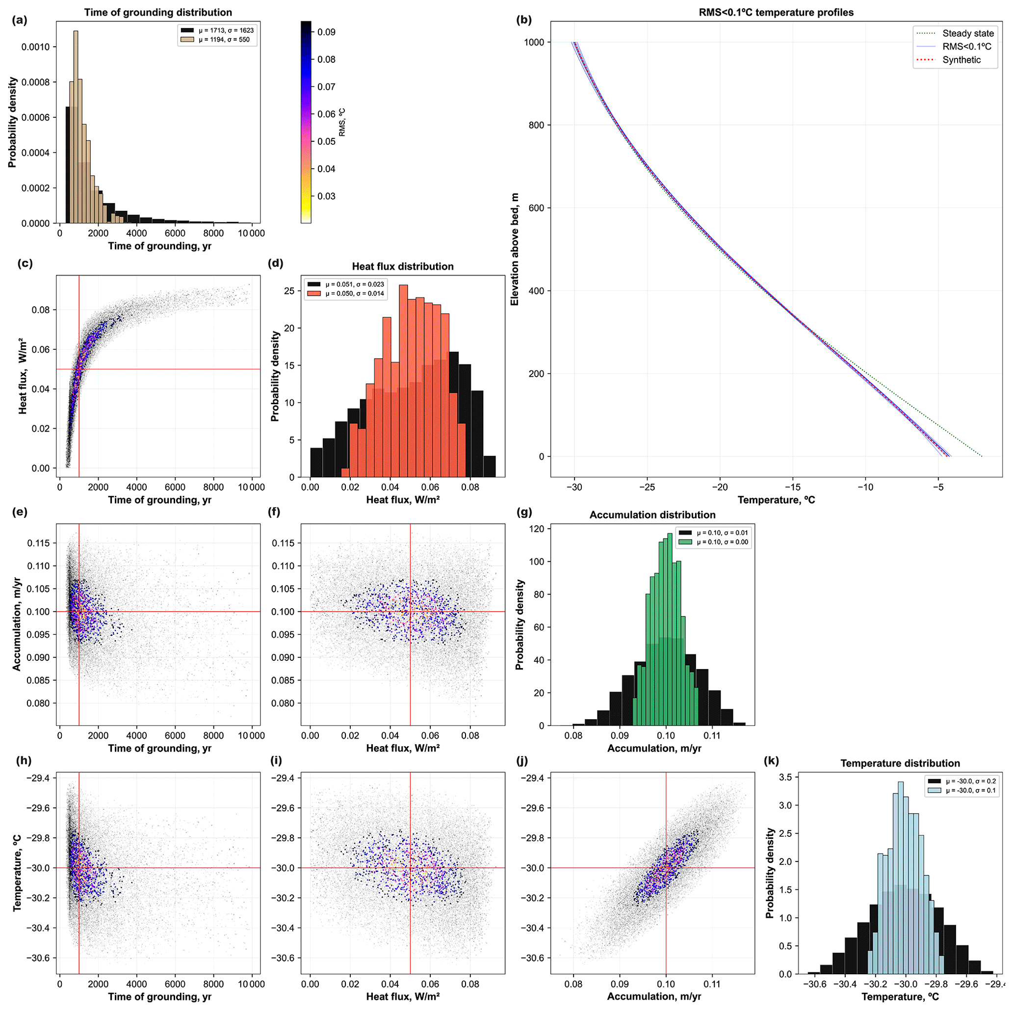
Figure 3 Inversion of the synthetic temperature profile data. Synthetic temperature–depth profile (dotted red line in panel b) was produced using the prescribed set of parameter values (shown by the intersection of solid red lines in the scatter plots, c, e, f, h–j). The scatter plots illustrate the random walk in the parameter space: in grey are the tested combinations of parameter values that yielded a less than 0.3 ^∘C rms misfit with synthetic temperature profile, while in colour is the combination of parameter values that yielded best-fit with synthetic profile (i.e. < 0.1 ^∘C rms). The colour of the points indicate the rms. Diagonally placed histograms (a, d, j, k) show posterior distributions for each parameter: black bars show parameter distributions that yielded rms < 0.3 ^∘C rms; coloured bars show distributions of parameter values that yielded best-fit with synthetic temperature profile (i.e. < 0.1 ^∘C rms). Insets in histograms display the mean, μ, and standard deviation, σ, of each distribution. (b) Randomly selected resultant temperature profiles for 0.1 ^∘C rms misfits.

3.1.2 Crary Ice Rise borehole measurements

To implement our MCMC inversion with englacial temperature data from Crary Ice Rise, we prescribe a wide range of prior values for model parameters. This allows us to probabilistically evaluate the possible combinations of realistic parameter values that could closely match the measured temperature–depth profiles (Fig. 4). For example, instead of assigning a heat flux of 77 mW m⁻², as used by Bindschadler et al. (1990), we obtain prior distributions of these values within a 200 km region around Crary Ice Rise using Martos et al.'s (2017) heat flux reconstruction (Sect. 2.1.3). Similarly, based on large-scale PISM model simulation outputs in the Crary Ice Rise area, we allow accumulation rates to vary between 5 and 20 cm yr⁻¹ (Fig. 4e–g). Here, our results are based on tests of 250 000 combinations of five parameters: surface temperature, accumulation rate, initial thickness, timing of grounding and geothermal heat flux.

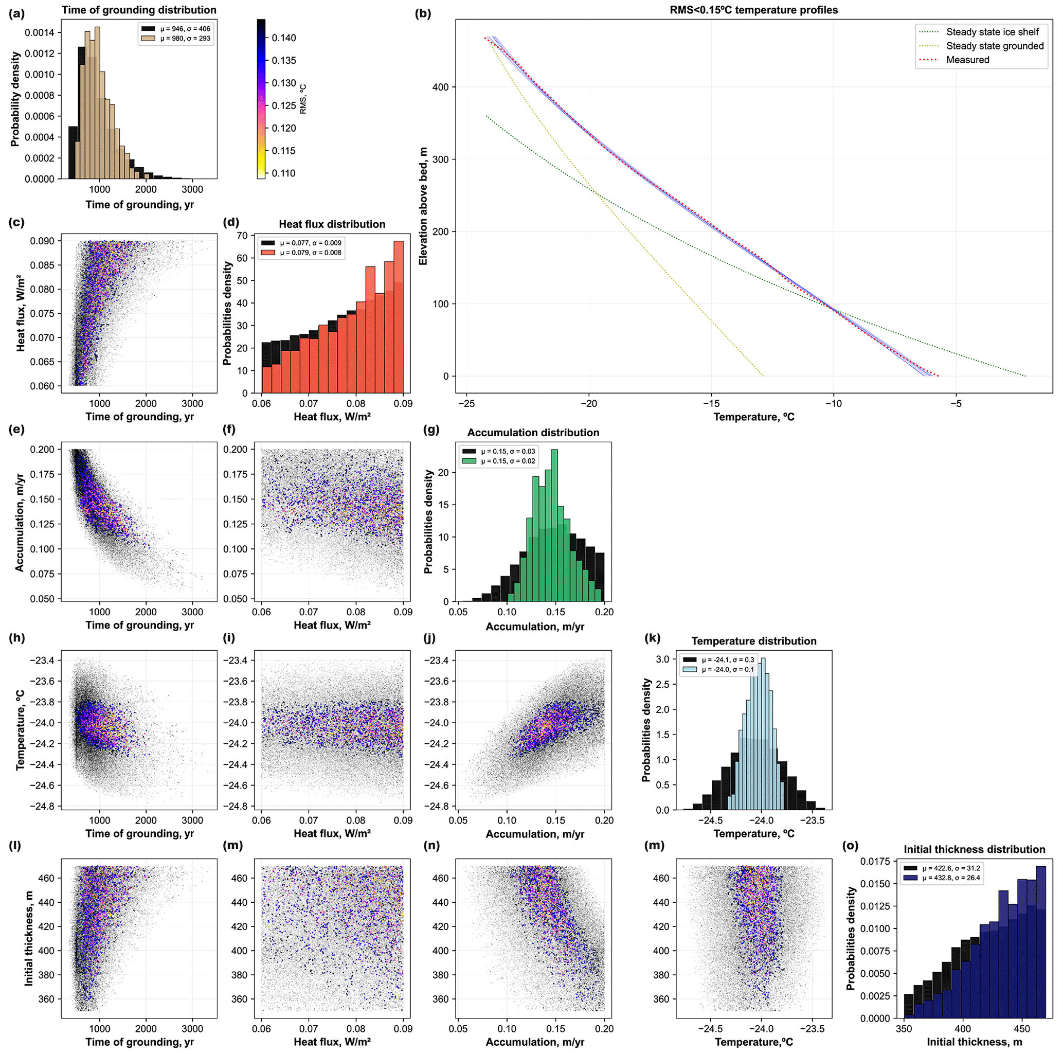
Figure 4 Inversion of the temperature–depth measurements near Crary Ice Rise Site D. Grey cloud of points illustrates the random walk in the parameter space, showing the tested combinations of parameter values that yielded a less than 0.3 ^∘C rms misfit with observations, while the coloured data points show the combination of parameter values that yields best-fit with measured temperature profile (i.e. less than 0.15 ^∘C rms). The colour of the points indicate the rms. Diagonally placed histograms (a, d, j, k, p) show posterior distributions for each parameter: black bars show parameter distributions that yielded rms < 0.3 ^∘C rms; coloured bars show distributions of parameter values that yielded best-fit with measured temperature profile (i.e. < 0.15 ^∘C rms). Insets in histograms display the mean, μ, and standard deviation, σ, of each distribution. (b) Randomly selected resultant temperature profiles for 0.3 and 0.15 ^∘C rms misfits.

Within the assigned prior parameter limits, the results show a wide range of posteriors that fit the observed temperature–depth measurements to within measurement errors reported by Bindschadler et al. (1990) (i.e. rms ∼ 0.1 ^∘C). Thus, over 25 000 samples yield a relatively low mismatch (i.e. 0.1 ≤ rms ≤ 0.15 ^∘C) with Crary Ice Rise measurements, with timing of grounding of 1000 ± 300 years (mean ± standard deviation; see Fig. 4a).

The distributions of the coloured points in the scatter plots in Fig. 4 provide insight into the dependence of each parameter and its uncertainty on the other parameters. For example, as with synthetic data inversion (Sect. 3.2.1), the inferred age of ice rise formation is strongly dependent on heat flux (Fig. 4c). Higher heat flux (i.e. about 90 mW m⁻²) yields grounding timing of 1400 ± 800 years, whereas lower heat flux of around 60 mW m⁻² implies earlier ice rise formation and lower uncertainties in the ice rise age estimations (500 ± 250 years). For comparison, using their deterministic least-square approach with fixed parameter values, Bindschadler et al. (1990) estimated an age of ice rise formation of 1100 years with a standard error between measured and simulated temperature profiles of 0.08 ^∘C. Our best-fit (i.e. rms of 0.1 ^∘C) temperature profile is inferred when the timing of grounding is 1300 years (with heat flux of 86 mW m⁻², accumulation of 0.14 m yr⁻¹ and initial thickness of 460 m being the estimated best-fit values). Here, we focus on the interplay between all parameters and do not assess the inferred initial thickness required to explain grounding at a particular Crary Ice Rise site. However, more extra information on past sea level, as well as the history of bedrock isostatic fluctuations, could easily be incorporated into our model to improve initial thickness estimation. Our MCMC inversion experiments highlight that the inferring timing of ice rise formation from englacial temperature measurements requires accurate knowledge of heat flux. However, Figs. 3 and 4 show that the inverse approach does not in full illustrate the sensitivity of the temperature profile to model parameters, and we discuss this in Sect. 3.2.

3.2 Englacial temperature profile sensitivity

To explore temperature profile sensitivity to model parameters and to identify which parameters are particularly important for ice rise dating and borehole thermometry, a series of forward simulations (Figs. 5a–c, 6) and Monte Carlo experiments (Fig. 5d–f) were conducted for each parameter under consideration. The resultant temperature profiles (Fig. 5a–c) were then directly compared for different ice thicknesses (Fig. 5d–f).

Figure 5 Englacial vertical temperature profile sensitivity to model parameters. (a, b, c) Example of five temperature profiles (with differences in the inset) obtained using a forward model for grounded ice with only the following parameter varied, while other variables remain constant at their mean value: (a) accumulation rate, (b) timing of grounding and (c) heat flux. (d, e, f) Results of forward simulations showing how a change (termed “delta” on the vertical axis label) in (d) accumulation rate of 0.01 m kyr⁻¹, (e) timing of grounding of 500 years and (f) geothermal heat flux of 1 mW m⁻² affects temperature profiles within grounded ice (expressed as root-mean-squared (rms) change between two profiles).

Figure 6 Englacial vertical temperature profile sensitivity to vertical velocity function and accumulation/surface temperature temporal variability. (a) Comparison of three temperature profiles obtained using a forward model for grounded ice with the Lliboutry, Dansgaard–Johnsen (with different values of “kink height” parameter z_k) and linear-vertical velocity approximations. (b) Comparison of four temperature profiles obtained using forward model for grounded ice with and without temporal variability of surface temperature and accumulation. (c) Comparison of three temperature profiles obtained using a forward model for grounded ice assuming three different thickening rates. (d, e, f) Results of forward simulations showing how much a range of ice-thicknesses temperature profiles differ depending on (d) various vertical velocity models, (e) temporally variable and constant parameters, and (f) ice thickening rates.

Temperature effects of changing heat flux and surface temperatures by a fixed value are similar for ice of a given thickness (e.g. for ∼ 2 km thick ice (average in Antarctica), a 1 mW m⁻² change in heat flux yields about 0.4 ^∘C (rms) change in temperature profile; see Fig. 5f). In contrast, fixed changes to accumulation rates and timing of grounding reflect a more complicated relation to resultant temperature profiles (Fig. 5d, e). For example, a 0.01 m yr⁻¹ accumulation change yields a considerably larger effect on englacial temperatures when accumulation rates are low (e.g. for a 2 km thick ice, about 0.4 ^∘C (rms) per 0.01 m yr⁻¹ for accumulation rates around 0.1 m yr⁻¹, compared to 0.1 ^∘C (rms) for accumulation rates of about 0.4 m yr⁻¹). In addition, higher accumulation rates lead to faster downward advection of surface temperatures and therefore increases the sensitivity of basal temperature to surface temperatures (Fig. 5a). Similarly, Fig. 5e shows that the temperature profiles are much more sensitive to grounding time for younger ice rises. Finally, changing temperature-dependent thermal conductivity value from 2 W m⁻¹ K⁻¹ (for ice close to the pressure melting point) to 2.6 W m⁻¹ K⁻¹ (for ice at −30 ^∘C) yields up to 0.3 ^∘C rms difference between the resultant temperature profiles for ice that is 500 m thick.

We also investigate how different velocity functions and temporal variability of thickness, accumulation and surface temperatures may affect the distribution of temperature within grounded ice of various thicknesses (Fig. 6). For these simulations, variable temperature and accumulation for the last 40 kyr were obtained from PISM simulation outputs (Fig. 1g–i). Advection effects of vertical velocity approximations on englacial temperature profiles are illustrated in Fig. 6a and d. Temperatures are affected most in the lower part of the ice column (Fig. 6a). Deviations between profiles produced with Dansgaard and Johnsen (1969) and Lliboutry (1979) velocity approximations also increase with ice thickness. For example, in 500 m thick ice the rms difference between two profiles is 0.18 ^∘C, while in 1800 m thick ice this difference is 2.55 ^∘C (Fig. 6d).

Inversion experiments described in Sect. 3.1 assumed constant surface temperatures, T_s, and accumulation rates, a, over the simulation period. To examine how temporal variability of these parameters impacts the temperature–depth data, we ran forward simulations and compared resultant profiles for four scenarios (T_s and a constant, T_s constant and a variable in time, a constant and T_s variable in time, both variable in time; see Fig. 6b). These experiments reveal considerable deviations between profiles forced only by one time-variable parameter, and while these effects typically do not exceed 1 ^∘C rms for ice thinner than 1 km, they result in as much as a few degrees rms difference between two profiles within ice about 3 km thick (Fig. 6b, e). The effect of the ice thickening rate is most significant in relatively thin ice (up to 2 ^∘C rms change for ice 500 m thick; see Fig. 6c, f) but decreases rapidly as ice becomes thicker.

Overall, forward sensitivity experiments outlined in this section provide insight into what model parameters have the strongest effect on the ice column, how these effects manifest in the shape of temperature profile and how this is affected by ice thickness. For thick ice, more likely to be found in the ice-sheet interior, parameters such as accumulation rates and the vertical velocity profile affect the temperature profile more strongly compared to thinner ice, more characteristic of ice-sheet periphery, including ice rises (Fig. 6). These results highlight the importance of careful vertical velocity parameterisation for borehole thermometry experiments in thick ice-sheet settings. In contrast, knowledge of ice-sheet thickening history is more important for dating shallow ice rises (Fig. 6c).

4 Discussion

4.1 Inversion of ice rise age

Bayesian inversion of englacial temperature–depth profiles indicates that inferences of ice rise age (i.e. timing of grounding) may significantly vary depending on the values of other forcing parameters. Among these, geothermal heat flux may have a significant effect on the inferred timing of grounding, with lower heat flux yielding earlier age estimates, along with much smaller corresponding uncertainties (that is, narrower range of solutions acceptable within a prescribed degree of misfit; see Figs. 3, 4). In the case of the Crary Ice Rise inversion experiment, we infer a range of possible ice rise age that encompasses the value of 1100 years previously reported by Bindschadler et al. (1990) but increases from 500 ± 250 to 1400 ± 800 years ago, as the corresponding values of heat flux decrease (assumed here to vary between 60 and 90 mW m⁻²).

The effect of heat flux may be significant when prior knowledge about its values is poor or unconstrained. For instance, in the synthetic data inversion experiment with prescribed grounding timing of 1000 years, heat flux of 30 mW m⁻² yields ice rise age estimation of 520 ± 80 years, whereas a value of 80 mW m⁻² corresponds to ice grounding 4030 ± 610 years ago, with both combinations falling within misfit of 0.1 ^∘C rms (Figs. 3, 7). This result is important, because previous deterministic approaches, for example, the one implemented by Bindschadler et al. (1990), assumed a fixed value of heat flux. However, recent studies have shown that despite its importance to understanding ice-sheet evolution (Pollard et al., 2005; Seroussi et al., 2017), heat flux beneath ice sheets remains relatively poorly constrained, with discrepancies between continental-scale reconstructions and targeted heat flux measurements and associated uncertainties of up to ±15 mW m⁻² (e.g. An et al., 2015; Martos et al., 2017; Fudge et al., 2019). Furthermore, heat flux at the base of an ice sheet may show substantial lateral variations (i.e. up to 200 mW m⁻²) over relatively short distances of less than 100 km, as for example observed below the Whillans Ice Stream (Begeman et al., 2017), as well as in other locations beneath the Antarctic and Greenland ice sheets (e.g. Cuffey et al., 1995; Dahl-Jensen et al., 2003; Schroeder et al., 2014; White-Gaynor et al., 2019). Careful estimation of heat flux uncertainties and their incorporation in temperature–depth inverse models are therefore essential for accurate estimation of past dynamic changes to ice rises.

Figure 7 Uncertainties associated with ice rise age inversion from temperature–depth profiles. (a) Combinations of values of heat flux and timing of grounding used in the synthetic inversion experiment that yield 0.1^∘ rms (mean indicated by orange line with light grey band around it indicating standard deviation) and 0.05 ^∘C rms (mean indicated by blue line with dark grey band around it indicating standard deviation) misfit with “measured” temperature profiles, respectively. (b) Temperature profile difference curves showing potential detectability of grounding-induced changes in the lower part of the ice column by repetitive englacial thermometry (for a time interval between measurements of 30 years for four different timings of grounding).

The uncertainties in ice rise age estimates are also determined by the degree of accepted misfit between predicted and measured temperature profiles, which in turn relies on the accuracy of englacial borehole thermometry. Depending on the instrumentation used, previous temperature–depth data have been collected with typical uncertainties of around 0.1 ^∘C (Orsi et al., 2012; Yang et al., 2017; Fudge et al., 2019) and occasionally up to 0.05 ^∘C and even 0.02 ^∘C, as demonstrated by work on the Antarctic Ice Sheet and Himalayan glaciers (Van Ommen et al., 1999; Miles et al., 2018; Talalay et al., 2020). Improvements in accuracy of measurements can put tighter constraints on inverted parameters: for example, in our synthetic data inversion experiments, decreasing uncertainties from 0.1 to 0.05 ^∘C more than doubles the accuracy of the inferred timing of grounding, as well as significantly narrows the range of accepted heat flux values (Fig. 7a).

Higher accuracy of englacial thermometry implies that the grounding-induced evolution of the temperature profile can be detected with two measurements separated by a few decades, which could potentially be utilised in previously drilled boreholes (Fig. 7b). In the case of Crary Ice Rise, a series of forward models shows that a 30-year increase in the timing of grounding (e.g. difference between temperature profiles within 1030 and 1000-year-old ice rise) may yield a difference in englacial temperatures that could be detected in the lower part of the ice column, as well as the upper section of the underlying sediment/bedrock (Fig. 7b). Therefore, if a sufficiently deep borehole is drilled, measurements through the underlying bedrock may provide useful additional constraints on both the heat flux and the timing of ice rise formation. However, following grounding, rapid attenuation of temperature differences with time implies that this method could only be applicable for ice rises that experienced recent grounding (i.e. less than around 1 ka), assuming measurement uncertainties of 0.02 ^∘C, as reported from a borehole drilled through the Dome Summit South in East Antarctica (Van Ommen et al., 1999). This loss of temporal resolution also implies increasing uncertainties associated with inferring the timing of grounding for ice rises that are older than approximately 4 kyr (Fig. 5e). Additionally, we do not take into account variations of thermal conductivity through the ice column. Temperature-dependent conductivity may yield a slight but measurable effect on the shape of englacial temperature profile, thus contributing to cumulative uncertainty in ice rise dating. Furthermore, our model does not account for the heating effects that may occur due to basal friction upon regrounding, as well as the freezing of groundwater and its corresponding effect on cooling. A more sophisticated forward model that takes this into account would be required to investigate this effect in water-saturated bedrock or sediments with high porosity.

4.2 Inversion of time-variable forcings

The Bayesian inversion method presented here has potential use in providing information about other model parameters, including time-variable thickness, temperature and accumulation rates, as previously done in multiple locations in Greenland and Antarctica (e.g. Dahl-Jensen et al., 1998, 1999; Waddington et al., 2005; Orsi et al., 2012; Cuffey et al., 2016). Since the addition of temporal variability to external forcings significantly increases the dimensionality of the inverse problem, with associated exponential growth of the computation cost, here we largely focus on thermal effects of dynamic ice rise evolution. However, our forward simulations show the variable impact of these forcings on englacial temperature distribution and their variability with ice thickness and depth within the ice column (Figs. 5, 6). For example, the effects of relatively small perturbations to accumulation rates are generally greater for thicker ice, whereas the opposite is true for timing of grounding and thickening rates, which play a more important role when ice is thin. Anomalies associated with changes to most parameters under consideration typically increase with depth (insets of Figs. 5a–c and 6a–d), with the exception of surface temperatures, which exert a strong influence on the temperature–depth distribution in the upper part of the ice column (e.g. Dahl-Jensen et al., 1998). This implies that the upper part of the ice column is likely to contain a more recent and less diffused record of past surface temperatures (e.g. Orsi et al., 2012).

Matsuoka et al.'s (2015) Antarctic ice rise inventory shows that ice rises rarely exceed 500 m in thickness (Fig. 1d), suggesting that these features may store a stronger signal of past dynamic changes and thickening history, whereas thick, permanently grounded ice domes may retain more information about accumulation and temperature histories and are thus more appropriate locations for palaeoclimatic inferences from englacial temperature measurements (e.g. Dahl-Johnsen et al., 1999; Engelhardt, 2004b; Orsi et al., 2012; Cuffey et al., 2016). Forward model experiments with different vertical velocity approximations show that the impact of vertical ice flow parameterisation becomes more significant for thicker ice (Fig. 6a, d). Yet, previous studies from Greenland and Antarctica have also shown that analytical ice flow approximations from Dansgaard and Johnsen (1969) and Lliboutry (1979) cannot fully capture the nonlinearity of vertical velocity profiles in ice divide/ice rise settings, and phase-sensitive radar measurements can provide useful additional constraints on vertical ice-sheet velocities (e.g. Gillet-Chaulet et al., 2011; Kingslake et al., 2014; Buizert et al., 2021). Therefore, integration of these techniques would help improve inferences of external forcings from borehole temperatures, in particular surface temperature and accumulation histories from deep boreholes.

4.3 Implications for choosing borehole drilling sites

Building on Bindschadler et al.'s (1990) foundational work and Neuhaus et al.'s (2021) more recent study, we have demonstrated how this method has potential as a useful dating technique that can be implemented at ice rises across Antarctica where direct geological sampling methods are inaccessible (e.g. Bentley et al., 2010; Spector et al., 2018). Integrating this technique with other methods, such as (1) indirect estimates of timing of grounding from radar observations and modelling (e.g. Schroeder et al., 2014; Kingslake et al., 2016; Wearing and Kingslake, 2019); (2) parameterisation of vertical velocities (Kingslake et al., 2014); and (3) adoption of more tightly restricted, informative prior constraints from geochemical ice-core data (e.g. for past temperature proxies; Cuffey et al., 2016) will allow for more accurate inferences of dynamic ice-rise/ice-sheet evolution and grounding line migration (e.g. Orsi et al., 2012). Moreover, we have demonstrated an approach for better quantifying uncertainties in these inferences. Borehole measurements through the upper tens of metres of underlying sediment/bedrock could place additional important constraints on both the geothermal heat flux and ice-rise evolution. This technique could even provide insights into dynamic ice-sheet evolution if future boreholes are drilled through floating ice and sediment in the vicinity of the grounding line, in places where recent ungrounding has left a pronounced vertical temperature anomaly within both ice and sediment/bedrock columns.

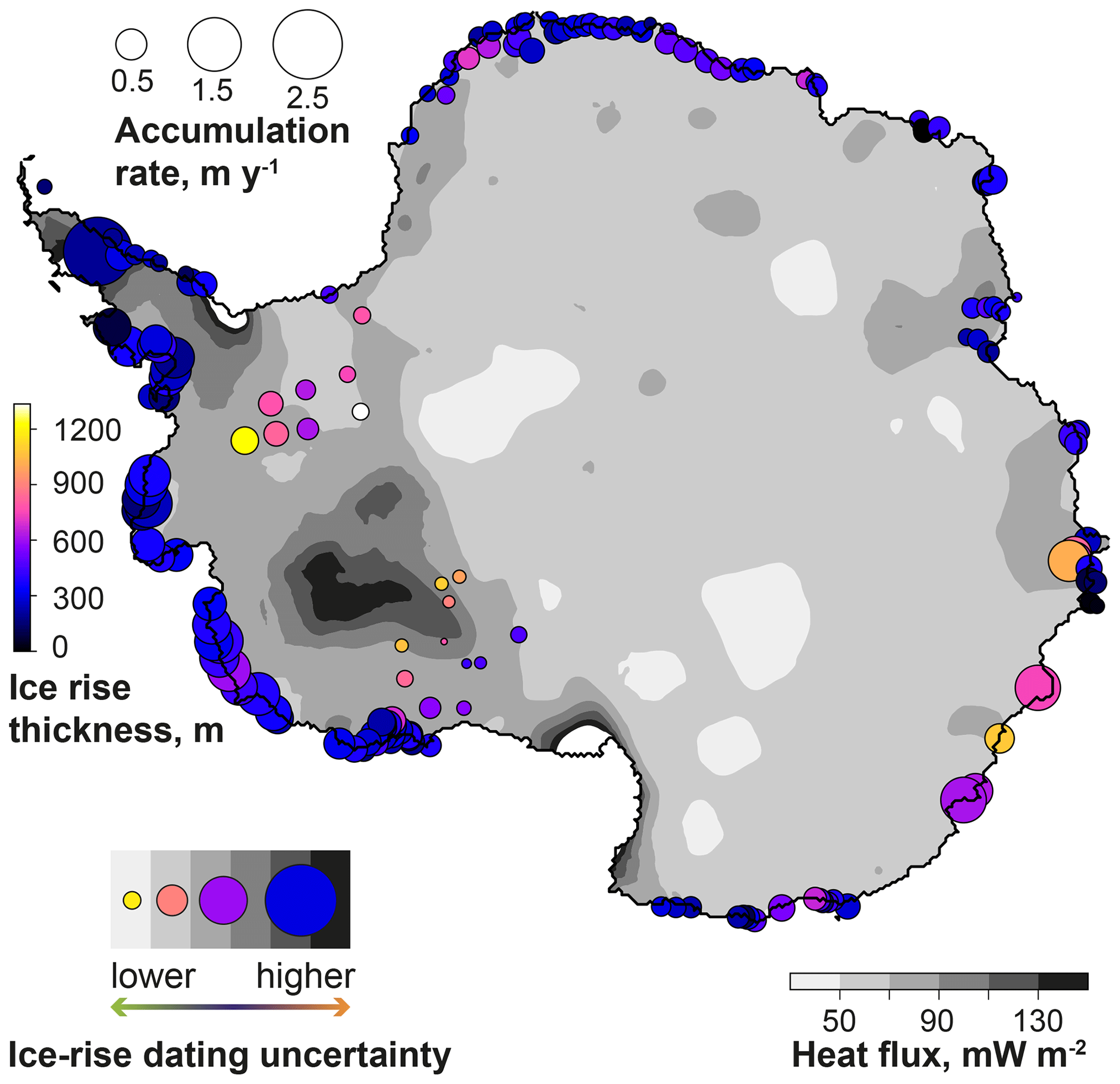
Figure 8 Antarctic ice rises and their suitability for dating of the potential Holocene ice-sheet regrounding. Circles correspond to the locations of ice rises from an Antarctic-wide inventory presented in Matsuoka et al. (2015). Sizes of the circles correspond to the mean present-day accumulation rates at their locations. Basemap shows distribution of basal geothermal heat flux presented in Martos et al. (2017). Areas where ice rise inverse dating techniques could be best applied are characterised by low heat flux, high ice thickness and low accumulation rates.

Our results prompt the question of what characteristics make a location favourable for borehole drilling and measuring temperature–depth data within an ice rise. Due to the diffusive nature of the englacial thermal signal, and as synthetic data experiments have shown, the temporal resolution decreases with time since grounding (Figs. 3, 5b, e, 7a). Therefore, ages of ice rises that are over 4 kyr old may be difficult to determine accurately, subject to other parameters like heat flux and thickening rates. Areas that are located close to the present-day grounding line, (and thus more likely to have been formed relatively recently) with well-constrained, low values of heat flux and low thickening rates, could represent optimal locations for implementation of this method and could yield accurate (i.e. on the order of 10 %) ice rise age estimations. Kingslake et al. (2018), Venturelli et al. (2020) and Neuhaus et al. (2021) have shown evidence of potential regrounding across large areas of West Antarctica. Preliminary investigations, juxtaposing these maps of potential grounding line migrations (Kingslake et al., 2018; Albrecht et al., 2020b) with Matsuoka et al.'s (2015) ice rise inventory (Fig. 1a–d) and Martos et al.'s (2017) heat flux model (Fig. 8) shows several ice rises where ice is relatively thick and accumulation rates are relatively low, for example Korff Ice Rise in the Ronne Ice Shelf area (Kingslake et al., 2016) and small ice rises to the east of the Weddell Sea. These ice rises could prove to be optimal locations for application of this technique. Future work could systematically quantify the suitability of these locations following this approach.

5 Conclusions

In this paper, we combine Bayesian inversion and forward modelling to make an evaluation of uncertainties inherent in inferences of ice rise dynamic evolution from temperature–depth profiles. Tested with both synthetic datasets and borehole temperature measurements from Crary Ice Rise, Ross Sea Embayment, our method explores the interplay between surface temperature, rates of accumulation and thickening, geothermal heat flux, and parameterised vertical velocities. We show that depending on the accuracy of borehole thermometry, the same temperature profile (within the accuracy of measurements) may result from a range of forcing parameters, of which geothermal heat flux through underlying bedrock plays a particularly important role. The key implication is that careful model parameterisation and evaluation of uncertainties are essential to infer dynamic ice rise evolution from borehole thermometry. We highlight that uncertainties in inferred ice-formation time may increase significantly with ice rise age. Accuracy of inversion relies on the low measurement uncertainties (i.e. < 0.05 ^∘C) and can be high (i.e. uncertainties < 10 %) for relatively young ice rises (i.e. formed < 4 ka) that are grounded in areas where heat flux is low, and its value is well constrained.