the Creative Commons Attribution 4.0 License.
the Creative Commons Attribution 4.0 License.
 | 05 May 2023
Impact of tides on calving patterns at Kronebreen, Svalbard – insights from three-dimensional ice dynamical modelling
Felicity A. Holmes
Eef van Dongen
Riko Noormets
Michał Pętlicki
Nina Kirchner
Understanding calving processes and their controls is of importance for reducing uncertainty in sea level rise estimates. The impact of tidal fluctuations and frontal melt on calving patterns has been researched through both modelling and observational studies but remains uncertain and may vary from glacier to glacier. In this study, we isolate various different impacts of tidal fluctuations on a glacier terminus to understand their influence on the timing of calving events in a model of Kronebreen, Svalbard, for the duration of 1 month. In addition, we impose a simplified frontal melt parameterisation onto the calving front in order to allow for an undercut to develop over the course of the simulations. We find that calving events show a tidal signal when there is a small or no undercut, but, after a critical point, undercut-driven calving becomes dominant and drowns out the tidal signal. However, the relationship is complex, and large calving events show a tidal signal even with a large modelled undercut. The modelled undercut sizes are then compared to observational profiles, showing that undercuts of up to ca. 25 m are plausible but with a more complex geometry being evident in observations than that captured in the model. These findings highlight the complex interactions occurring at the calving front of Kronebreen and suggest further observational data and modelling work is needed to fully understand the hierarchy of controls on calving.
- Article
(6957 KB) - Full-text XML
- BibTeX
- EndNote


Worldwide, glaciers have been losing mass during recent decades, with these mass losses contributing to eustatic sea level rise. Different elements of the cryosphere are contributing varying amounts; between 2006 and 2015, Greenland contributed 0.77 mm yr−1, glaciers non-peripheral to Greenland and Antarctica (including Svalbard) 0.61 mm yr−1, and Antarctica 0.43 mm yr−1 (IPCC, 2022). One of the biggest hurdles to effective management of and adaptation to rising sea levels is having good projections of the future. To produce those, increased understanding of certain glaciological processes is required, especially along the marine ice margins. Mass loss originating from these areas is of significance; it is estimated that between 32 % and 67 % of mass loss from Greenland is due to calving (Rignot and Kanagaratnam, 2006; Enderlin et al., 2014). When considering both calving and submarine melt (which, when combined with subaerial melt and sublimation at the calving front, constitutes frontal ablation), around one-third of Greenland's net mass loss between 2000 and 2012 can be attributed to their combined effect (King et al., 2020). Since 2013, this contribution has been over 50 % as a result of a less negative surface mass balance (King et al., 2020). For Svalbard, estimates have put the contribution of calving in the range of 17 %–25 % of total mass loss (Błaszczyk et al., 2009). No more recent studies have been conducted to give updated estimates of calving fluxes for the whole of Svalbard, but the retreat of Svalbard's tidewater glaciers over recent decades implies significant calving (Braun et al., 2016; Schuler et al., 2020). Added to this, studies on individual glaciers have shown considerable variability in calving losses with, for example, the 2012–2013 Austfonna surge potentially causing a doubling in the frontal ablation losses from Svalbard for this period and highlighting the need for updated estimates of frontal ablation (Dunse et al., 2012; Schuler et al., 2020). Also, there is evidence that submarine melting may be of considerable importance for the frontal ablation of Svalbard glaciers (e.g. Luckman et al., 2015). In Antarctica, both melting from the ocean and calving and/or ice-shelf collapse have had large impacts on overall mass loss in recent decades (Shepherd et al., 2018). Between 1992 and 2017, submarine melt led to an annual increased ice loss in West Antarctica of 106 ± 55 ×109 t (Shepherd et al., 2018). During the same time period, ice-shelf collapse led to an increased mass loss of 26 ± 29 ×109 t yr−1 from the Antarctic Peninsula (Shepherd et al., 2018). Improved understanding of calving events and their triggers is crucial as calving and frontal melt have been shown to impact upstream glacier dynamics, through a positive feedback loop causing acceleration, thinning, and further retreat as earlier described for Jakobshavn Isbrae after the breakup of its ice tongue (Holland et al., 2008; Price et al., 2011; Christoffersen et al., 2011).
Mass losses at the ice–ocean interface from calving and submarine melt have been linked to increasing ocean temperatures (Christoffersen et al., 2011; Luckman et al., 2015; Holmes et al., 2019). However, atmospheric temperatures are also of importance through their ability to increase surface melt levels. This surface melt can then make its way into the subglacial hydrological system, where it is combined with water produced by basal melting (Karlsson et al., 2021). These waters subsequently exit the glacier at its terminus as a buoyant plume which rises through the water column whilst turbulently entraining warm waters residing at depth, if present, and exacerbating melt (Jenkins, 2011; Slater et al., 2017).
Alongside ocean and atmospheric temperatures, various other variables can act to trigger or modulate frontal ablation. For example, fjord topography and bathymetry can stabilise glacier fronts or block the intrusion of warm waters which might otherwise reach the grounding line where they could cause enhanced submarine melt (Jakobsson et al., 2020; Holmes et al., 2021). Sea level fluctuations, most notably due to tidal phase (falling vs. rising tide), and ice mélange buttressing are examples of other factors which have received interest with regards to their importance for modulating the occurrence of calving (e.g. Todd and Christoffersen, 2014; Bartholomaus et al., 2015; How et al., 2019) with potential knock-on impacts on frontal glacier velocity (Walters and Dunlap, 1987; Walters, 1989; Podrasky et al., 2014).
Here, we aim to provide some insight into how changing sea levels and frontal melt may influence calving patterns at Kronebreen, Svalbard, via the use of numerical modelling. We start from a simulation where the combined effects of tidal variations, frontal melt, and calving are all included. We use tidal input data from August 2016 due to the availability of observations of both the subaerial and submarine portions of calving front morphology from the 16 August 2016, providing a rare opportunity to compare modelled and observed calving front geometry. However, due to simplifications in the model set-up that allow us to isolate tidal impact, the results are best viewed as a conceptual study that allows comparison of undercut magnitude rather than a direct representation of conditions during this time period. The various impacts of tidal fluctuations on calving are then investigated, with the effects of changing back pressure, changing water levels in crevasses, and changing frontal melt locations all being tested separately. Through the use of various different frontal melt scenarios, the experiments presented here additionally allow for an evaluation of the impact of terminus geometry on modelled calving patterns, something which has not been extensively studied previously.
Kronebreen, located on the west coast of Spitsbergen at 78.8∘ N, 12.6∘ E, is a fast-flowing, grounded glacier (see Fig. 1). Near its ca. 3.6 km wide terminus (Holmes et al., 2019), Kronebreen shares a lateral margin with the much slower neighbouring glacier Kongsvegen, with both glaciers then terminating in Kongsfjorden. Kronebreen is fed by Holtedahlfonna and Infantfonna, with a total combined area of 372 km2 (Schellenberger et al., 2015). In Kronebreen's lower reaches, it is heavily crevassed with flow speeds that can reach up to 5 m d−1 during summer (Schellenberger et al., 2015). Velocities, however, vary both seasonally and interannually, with these fluctuations attributed to the seasonal development of the basal hydrological system and variations in surface melt (Schellenberger et al., 2015; Vallot et al., 2017). Kronebreen has experienced increasing levels of melt in recent decades, with surface melt during 2000–2012 having increased by 21 % when compared to data from 1961–1999 – likely as a consequence of increased atmospheric temperatures (Van Pelt et al., 2012). Kongsfjorden has a length of 22 km and a width of between 4 and 12 km, making it wide enough for the Coriolis force to impact on circulation (Svendsen et al., 2002; Trusel et al., 2010). Kongsfjorden does not have a defined sill but does exhibit variable bathymetry that ranges from ca. 400 to ca. 60 m. The fact that there is no defined sill means that intrusions of warm Atlantic water (>3 ∘C) are able to enter Kongsfjorden and, potentially, reach the calving front of Kronebreen (Svendsen et al., 2002). Kongsfjorden's location on Svalbard's western coast means that it is in close proximity to the West Spitsbergen Current and so is subject to a wide range of different water masses (Nilsen et al., 2008). Previous work in the area has confirmed the presence of Atlantic waters in the fjord, with potential impacts for Kronebreen and neighbouring glacier Kongsvegen (Cokelet et al., 2008; Promińska et al., 2017). The water masses present in the fjord vary both seasonally and between years as the proportions of Arctic waters, Atlantic waters, and glacially derived waters do not remain constant. Due to this variability, Kongsfjorden can either be in a “cold mode” or a “warm mode” depending on the amount of Atlantic water present (Cottier et al., 2005). From investigation of optical satellite imagery, two distinct subglacial plumes can be identified at the terminus of Kronebreen: one in the north and one in the south (see Fig. 1). Previous studies have found that the frontal ablation rate of Kronebreen is strongly correlated with fjord water temperatures, suggesting that fjord circulation and the aforementioned subglacial plumes are likely important drivers of mass loss at the terminus (Luckman et al., 2015; Holmes et al., 2019). In addition, a mass budget for Kronebreen between 2009 and 2014 found that frontal ablation accounted for around 84 % of total mass loss (Deschamps-Berger et al., 2019).
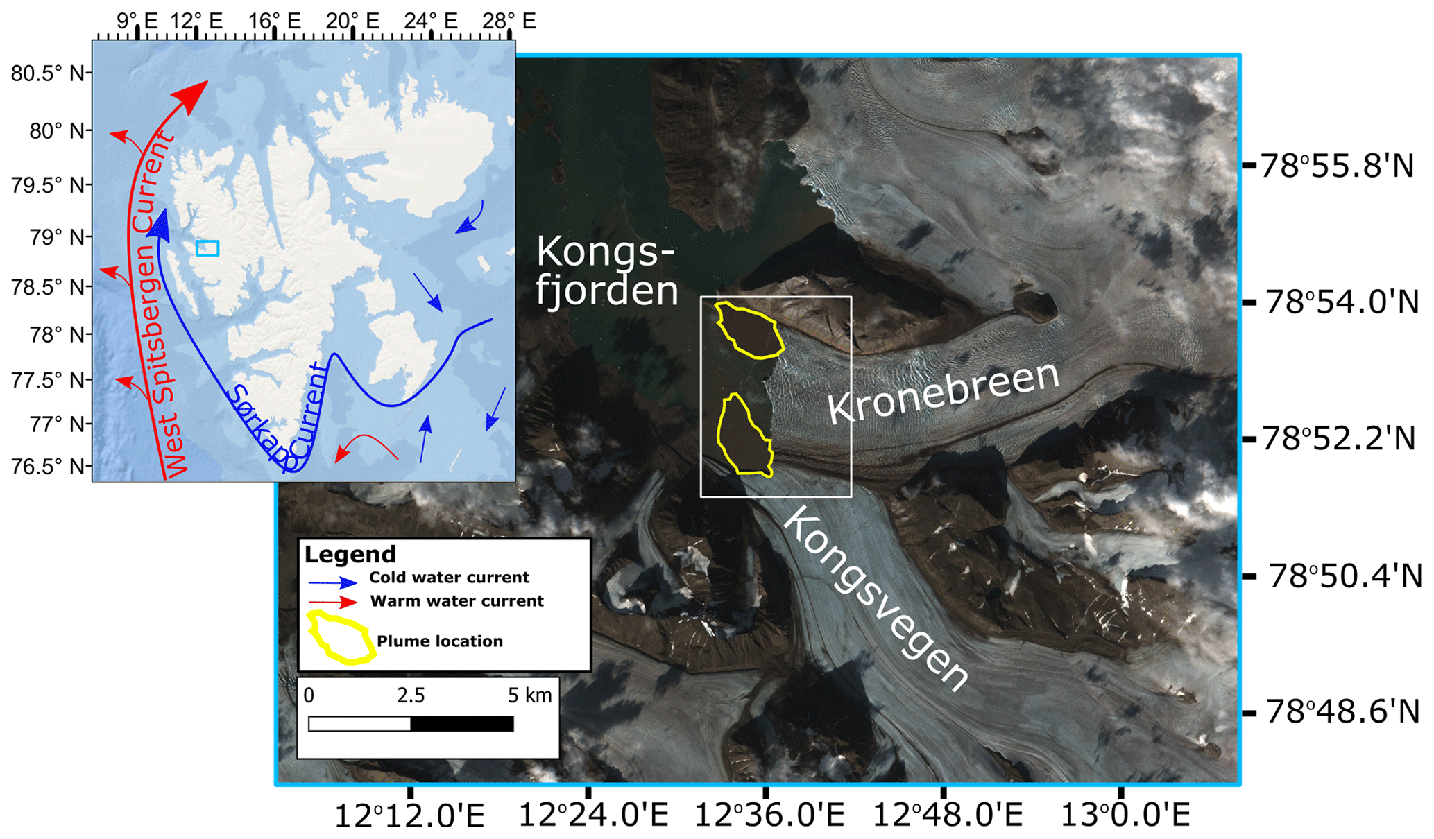
Figure 1Location of Kronebreen on Svalbard (inset) and close-up showing the heavily crevassed frontal section of Kronebreen, as well as Kongsfjorden and Kongsvegen from August 2016 (right). The West Spitsbergen Current (warm waters, red) and Sørkapp Current (cold waters, blue) are adapted from Sundfjord et al. (2017) and shown on the inset figure. Main image: the yellow polygons denote the location of subglacial plumes. The white box delineates the area shown in Fig. 4a. Main image source: Copernicus Sentinel data (2022). Retrieved from Copernicus Open Access Hub on 23 May 2022, processed by ESA. Inset background image source: Esri, DigitalGlobe, GeoEye, Earthstar Geographics, CNES/Airbus DS, USDA, USGS, AeroGRID, IGN, and the GIS user community.
Observational data from August 2016 provide motivation for the modelling experiments conducted here. These model experiments are, however, primarily designed to investigate model behaviour rather than to reproduce observed glacier behaviour.
3.1 Observational data
3.1.1 Calving front morphology
Two profiles showing the frontal geometry of Kronebreen were mapped using a Kongsberg EM2040 multibeam (MB) echosounder and a Riegl VZ-6000 terrestrial lidar on the 24 August 2016 (see Fig. 2). The MB was mounted on a small research vessel in Kongsfjorden and acquired imagery of the submarine morphology of the calving front. The lidar scanner was mounted on the southern shore of Kongsfjorden, at 78∘52′04.1′′ N, 12∘29′06.7′′ E, to image the calving front's geometry above the waterline.
The Riegl VZ-6000 lidar is equipped with a long-range near-infrared laser and uses the time-of-flight principle to calculate a distance to the measured object. For the Kronebreen subareal ice cliff survey, the pulse repetition rate (PRR) was set to 50 kHz, and the horizontal and vertical angular resolutions were set to 0.0045∘, resulting in a nominal spatial resolution of ca. 5 cm at the distance of 1.5 km. However, due to unfavourable meteorological conditions, the survey geometry, and poor reflection from the ice cliff, the effective resolution was limited to ca. 80 cm in horizontal direction and approx. 30 cm in the vertical. The instrument has a nominal distance accuracy of 10 mm and precision of 15 mm at a range of 150 m. The lowermost part of the cliff, in constant contact with wave action and water spray, has very low reflectivity in the near-infrared part of the spectrum, and therefore no laser return was obtained at the waterline. Overall, based on previously published surveys of the ice cliffs, we conservatively estimate the measurement uncertainty at 30 cm.
The EM2040 is a wide-band, high-resolution, shallow-water MB echosounder with one 0.4∘ wide transmit beam and 256 0.7∘ wide receiver beams, operated at a frequency of 200 kHz. Sampling frequency varied between 5 and 10 Hz and was limited by water depth. The range resolution was usually within 1 to 2 cm. The EM2040 was coupled with Kongsberg’s Seapath 330+ Global Navigation and Satellite System positioning and motion reference units. Positioning was aided by a local real-time-kinematic reference station placed on a nearby coastal area. As a result, positioning accuracy was better than 10 cm.
The two profiles, one shown in green and one in orange in Fig. 2, consist of 1211 and 1006 points respectively, with both transects running from easting 448000 to 448060 (UTM zone 33N). Soundings were taken between northings 8756133 and 8756134 (green profile) and northings 8756633 and 8756634 (orange profile). These data allow for comparison of undercut sizes between the model and observations, but, due to the conceptual nature of the model, smaller-scale morphologies cannot be compared. The green profile corresponds to the location of a subglacial plume, as identified from satellite imagery. The orange profile does not correspond to a satellite-identified plume location.
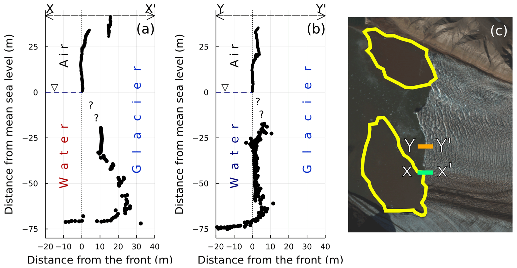
Figure 2(a) Frontal geometry at the X–X′ (green) profile of Kronebreen as observed from MB and lidar at the location denoted by the green line on panel (c). (b) Frontal geometry at the Y–Y′ (orange) profile of Kronebreen as observed from MB and lidar at the location denoted by the orange line on panel (c). Panel (c) shows the location of the two profiles, as well as of the subglacial plumes identified from satellite imagery (yellow polygons). Background image: Copernicus Sentinel data (2022) from 22 August 2016, 2 d before the MB/lidar data were collected. Image retrieved from Copernicus Open Access Hub on 23 May 2022, processed by ESA.
3.1.2 State of Kronebreen and surrounding areas during 2016
To guide the model set-up and evaluation, several observational and model-derived data sets were compiled. This included glacier velocities, 2 m air temperatures, and tidal fluctuation data.
Ice surface velocities are calculated from Sentinel-1 GRDH SAR (ground-range-detected high-resolution synthetic aperture radar) images (Copernicus Sentinel data, 2016) via offset tracking (e.g. Strozzi et al., 2002) of orbitally corrected and co-registered image pairs with a grid azimuth and range spacing of 10 pixels, corresponding to a resolution of 100 m. A summer (3–15 July 2016) and a winter (30 November to 6 December 2016) velocity field were calculated. The errors of the frontal surface velocity fields were estimated at around 0.3 m d−1 by looking at movement vectors on known stationary objects such as mountains. In addition, a time series of velocities and frontal ablation during 2016–2017 are presented by Holmes et al. (2019) and can be used to compare bulk frontal ablation rates between the model and observations.
Surface air temperature (2 m), as well as surface mass balance (SMB) and its component parts (snowfall, rain, runoff, refreezing and retention, and melt), are provided in a data set by Noël et al. (2020) at a 500 m spatial and daily temporal resolution and cover both summer 2016 and winter 2016–2017.
Tidal fluctuations from measurements taken every 10 min at Ny-Ålesund, Svalbard (ca. 17 km from Kronebreen's terminus), were collected from https://kartverket.no (last access: February 2022) and define the temporal changes of sea level in the model. The data from kartverket.no are provided with reference to the mean water level observed during the period 1996–2014.
3.2 Modelling domain and set-up
This modelling study was carried out using Elmer/Ice (version 9.0), a finite-element, full-Stokes, three-dimensional ice-sheet and glacier-flow model (Gagliardini et al., 2013), with a calving implementation based on the calving depth criterion (Benn et al., 2007; Todd et al., 2018). The code for Elmer/Ice is open source and freely available at https://github.com/ElmerCSC/elmerfem (last access: February 2022).
The model domain (Fig. 3) is based on that used by Vallot et al. (2018) but altered to give the calving front its satellite-derived summer 2016 position. This was done to provide some consistency between the model domain and the tidal forcing, which is derived from observations taken in August 2016. However, the model set-up is designed to be diagnostic of how tides impact calving in the Elmer/Ice calving model rather than to represent a certain time period as accurately as possible. The calving model in Elmer/Ice ignores the yield stress required to open crevasses but, as a result of Kronebreen being heavily crevassed near its terminus, this can be justified (Todd et al., 2018). Mesh resolution varied from 100 m at the front to 2000 m at locations furthest from the calving front (Fig. 3). A separate 2D planar mesh is created over the frontal area in order to determine crevasse propagation (Todd et al., 2018), and, for this planar mesh, a higher resolution of 10 m was used to allow for small calving events to be identified. The main 3D mesh was internally extruded to have 10 vertical layers, rendering a resolution of ca. 10 m at the front. Five different types of mesh boundaries were implemented: an ice–ocean boundary (at the calving front), an ice–ice boundary (e.g. the confluence of Kongsvegen and Kronebreen), an ice–rock boundary (at the fjord walls), and the basal and the upper surface of the glacier, derived from data by Lindbäck et al. (2018) over the course of several years, implying some mismatch between glacier thickness in the model and in reality and thus providing motivation for viewing the results as primarily indicative of model behaviour. At the ice–ice boundaries (for instance the confluence of Kronebreen with Kongsvegen), velocities were prescribed to match those derived from offset tracking of satellite images (see Sect. 3.1.2). At the ice–rock boundaries, velocities were set to 0.0 under the assumption that movement is very limited here. In the majority of simulations, a linear-type Weertman (1974) friction law is applied at the base, as has been done for several previous studies investigating calving using Elmer/Ice (e.g. Todd et al., 2018, 2019; Cook et al., 2020). However, in light of evidence that a Weertman-type sliding law can be problematic at Kronebreen (Vallot et al., 2017) and that tidal response may depend on effective pressure (Amundson et al., 2022), a simulation was also run with a Coulomb sliding law (Schoof, 2005; Gagliardini et al., 2007). In all simulations, stress-free conditions are prescribed at the surface. For each tidal simulation, the entire month of August 2016 was simulated using a 10 min time step. Different time step sizes and simulation lengths were used for the spin-up and relaxation simulations (see Sect. 3.4).
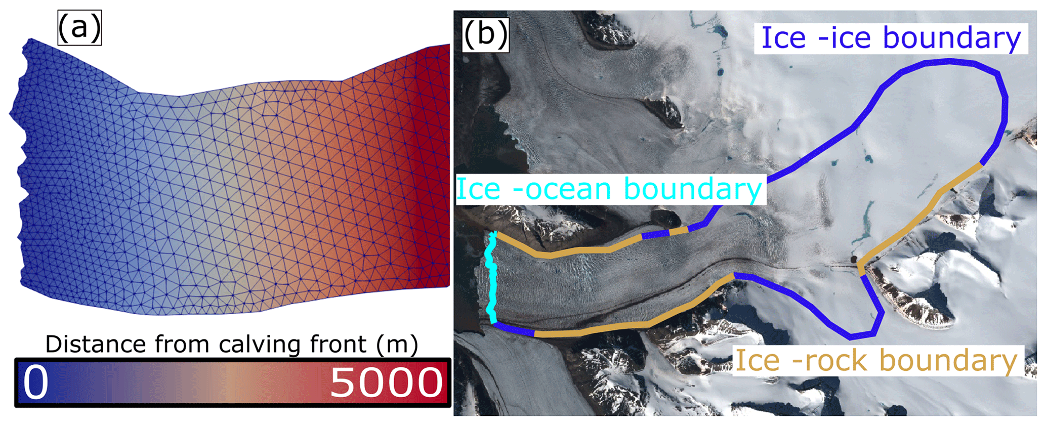
Figure 3(a) View of frontal part of the mesh from above, with the different element sizes shown, which are smallest at the calving front and get larger with distance from the calving front. (b) The mesh domain and boundaries are shown, overlain on a Sentinel-2 satellite image. The glacier margin is ca. 3.3 km wide and the distance along a central flowline is ca. 28 km. Background image for panel (b): Copernicus Sentinel data 2016, retrieved from Copernicus Open Access Hub on 23 May 2022, processed by ESA.
3.3 Model inputs
For model initiation and model forcing during the simulations, four variables are of particular relevance: satellite-derived surface glacier velocities (for basal friction inversions and inflow velocities at the ice–ice boundaries), surface temperatures (for use in the thermodynamic spin-up), sea level (tidal) fluctuations (for use as a forcing in the main suite of simulations), and submarine frontal melt (FM; to account for the impact of oceanic heat on processes at the calving front). No subaerial melting or sublimation of the calving front above the waterline was included. The required velocities, air temperatures, and tidal fluctuations were harvested from the data sources specified in Sect. 3.1.2.
As the tidal fluctuations cover an entire month, tidal amplitude varies over the course of the simulations with both spring and neap tides being present. For the isolation of tidal impacts, changing water levels in the model imply changes relating to the following:
-
where sea pressure (SP) is exerted, with sea pressure exerted over a greater proportion of the calving front when the tide is high, leading to greater overall pressure exerted on the calving front during high tides;
-
where frontal melt (FM) occurs, with a greater proportion of the calving front experiencing frontal melt during high tides – changes in fjord circulation or ocean heat transport as a result of tidal fluctuations are not included;
-
the depth to which crevasses must propagate to cause a calving event (CD), as calving occurs when crevasses reach sea level, and this required propagation distance is minimised when sea level is higher as a result of high tide.
For simulations where FM was applied, its location and magnitude were kept constant during the simulations. The background level of melt was set to 500 m yr−1, and the high-melt (plume) level was set to 1500 m yr−1. As such, frontal melt was prescribed across the entire submerged part of the terminus. Previous estimates of FM at Kronebreen have suggested winter lows ranging from ca. 30 to ca. 400 m yr−1 and summer highs ranging from ca. 300 to ca. 2300 m yr−1 (Holmes et al., 2019; Köhler et al., 2019). As a summer scenario is in focus here, the background and plume melt values were chosen so that they fit within the summer FM estimate range. However, the FM parameterisation used here is simple, and further study is needed to better constrain frontal melt rates at Kronebreen. The location of the high-melt (plume) areas along the calving front (Fig. 1) was informed by the visual inspection of optical Landsat 8 satellite images from 2016 and 2017. Around one-third of the submerged calving front was subject to the higher plume melt rates, but this proportion varied as a consequence of calving events changing the total surface area of the terminus. FM is, by definition, only applied below the waterline, with values of 0 m yr−1 prescribed for subaerial parts of the terminus. These FM values allowed for an undercut to develop during the course of the simulations, providing insight into how frontal morphology may impact calving. However, the simplified melt parameterisation is likely to lead to sharp corners and associated high stresses which may lead to an overestimation of calving.
3.4 Simulation workflow
The workflow consisted of five stages: (I) inversions for basal friction; (II) a fixed-geometry 500-year thermodynamic spin-up; (III) a 125 d relaxation simulation with calving and front movement permitted; (IV) the main simulations, a suite of 10 runs, with a freely evolving ice surface and fully active calving front; and (V) post-processing, during which the percentage of calving events in each simulation occurring on a rising tide and a falling tide was investigated, both for calved icebergs of any size and for large (>500 m3) icebergs. In addition, the absolute water depth at which calving events occurred was investigated, and calving frequency was related to tidal amplitude.
In numerical ice flow simulations, basal friction has to either be prescribed or be computed from observed ice surface velocities using inverse approaches (e.g. Gillet-Chaulet et al., 2012; Vallot et al., 2017). Here, we follow Arthern and Gudmundsson (2010), who employed the Robin inverse method to invert surface velocities for basal friction, now distributed as part of Elmer/Ice (cf. Sect. A1 and Fig. A1). Separate inversions were done for winter and summer using velocity fields derived from offset tracking (see Sect. 3.3), as levels of basal and surface melt vary seasonally and can lead to large variations in basal friction at Kronebreen (Vallot et al., 2017). Basal friction, a parameter in the Weertman sliding law, was subsequently modelled as a sinusoidally varying curve with the two inverted fields as maximum and minimum values during stages II and III. The maximum field was from winter (30 November 2016 to 6 December 2016) and the minimum field from summer (3 July 2016 to 15 July 2016; see Fig. A2). In the simulation with a Coulomb sliding law, the friction coefficient was determined by a re-scaling of the inverted basal friction field in order to match observed velocities at Kronebreen (e.g. Joughin et al., 2019).
A fixed geometry spin-up simulation with temperature forcing corresponding to average temperatures for the years 2000–2018 was then run. The only output variables that were allowed to develop with time were velocity and temperature (e.g. Sato and Greve, 2012; Seddik et al., 2012). The spin-up was run for 500 years at monthly time steps until reaching a steady state, which was identified from the lack of a directional trend in the time series of temperatures and velocities (cf. Sect. A1). The temperature field was forced with surface temperatures, and took frictional heating into account, but does not include firn warming by refreezing of meltwater despite its recorded importance for Svalbard glaciers (van Pelt et al., 2016).
As fixed geometry spin-ups can lead to artificial drift after surfaces are allowed to evolve (Le clec'h et al., 2019), a relaxation simulation was run for 500 time steps of 0.25 d each after the spin-up (cf. Sect. A1 and Fig. A2). In this step and for all further steps, the temperature field was set to be constant and equalled the results of step II. For the relaxation simulation, there was still no SMB forcing, but calving and frontal melt (at a constant 500 m yr−1) were activated to allow for relaxation of the terminus geometry. These simulations used the Calving3D solver, which is based on the calving depth criterion (Benn et al., 2007), implemented into Elmer/Ice and evaluated for Store Glacier, central West Greenland, by Todd et al. (2018). This solver facilitates calving via one of two mechanisms: either surface crevasses and basal crevasses meet and imply fracture from the surface to the base (mechanism “base”) or surface crevasses extend to the waterline where crevasse propagation to the ice base takes place through hydrofracture (mechanism “surf”). To accommodate for changes in calving front geometry induced by calving events, the 3D mesh is updated after each calving event. In this stage, only limited calving was permitted by limiting the area over which calving could occur to points within 50 m of the terminus.
The modelled configuration of Kronebreen at the end of stage III served as a starting point for the 10 main simulations in stage IV (see Fig. A2). These have in common that they were each run for 31 d, at a time step of 10 min wall clock time. No SMB forcing was included, and frontal melt (now including plumes) was kept temporally constant throughout each of the simulations in order to allow for isolation of the tidal impacts. The 31 d of modelled glacier evolution in each simulation span the month of August 2016 but, due to model design, are not a direct analogue for conditions during this period and should instead be viewed as diagnostic simulations.
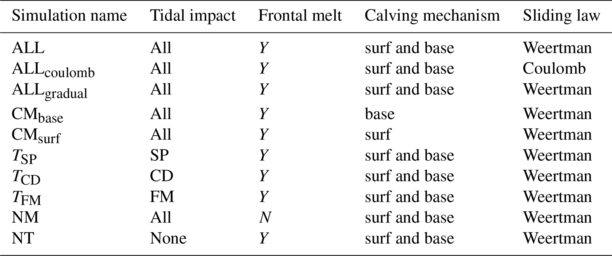
The 10 runs are summarised in Table 1. Simulation ALL serves as a control run and includes all identified tidal impacts described in Sect. 3.3 (FM, CD, and SP), both calving mechanisms (surf and base), and frontal melt. By switching off selected mechanisms (see Sect. 3.3), six different simulations are designed to isolate the impacts of calving mechanisms (CMbase, CMsurf), tidal fluctuations (TSP, TCD, TFM), and (absence of) frontal melt (NM). In addition, the ALLcoulomb simulation was run, which is identical to the ALL simulation except in the fact that a Coulomb sliding law, rather than a Weertman sliding law, was prescribed at the base. A simulation was also run with a frontal melt which gradually increased from the waterline down to 30 m, in order to create a more gradual undercut (ALLgradual). Finally, one simulation was run with no tidal fluctuations in water level (NT).
For step V, post-processing, the occurrence of calving events was related to tidal cycles in a number of different ways. Firstly, the percentage of calving events occurring on rising or falling tides was calculated for both icebergs of all sizes and for large (>500 m3) icebergs. This threshold was chosen as it corresponds to 5 % of total icebergs. For these results, hypothesis testing (binomial distribution, one-tailed) was conducted with any results, where p<0.05 was considered statistically significant.
In addition, the water depth (deviance from mean sea level) at which calving events occurred was investigated to look for a pattern between, e.g. low or high water levels and calving regardless of whether water levels are rising or falling. By looking at temporal variations in calving, the occurrence of calving was also related to tidal amplitude (spring vs. neap tides).
Finally, a frontal ablation rate was calculated for each simulation by taking the total ice volume loss (m3) from both calving and frontal melt and converting it into metres per day (m d−1) by using estimates of Kronebreen's terminus geometry (width and height).
Table 1Summary of processes included in the suite of tidal simulations. Possible tidal impacts are SP (sea pressure), CD (crevasse depth), and FM (frontal melt) and are described in more detail in Sect. 3.2. The calving mechanisms “surf” and “base” are described in more detail in Sect. 3.3.
For all 10 main simulations (Table 1), the percentage of calving events occurring on a rising tide and a falling tide are shown in Table 2, with separate values for all icebergs and for large icebergs. Percentages are used to quantify the occurrences because the absolute number of calving events differs between simulations. The mean number of calving events in all 10 simulations was 2074, corresponding to an average of 67 events per day or 2.8 events per hour. It can be seen that, when considering icebergs of all size, there is no clear preference for calving on a particular tidal phase. However, when focusing on large icebergs, a clear tidal signal can be seen in most of the simulations. Specifically, ALL, CMbase, and NM show a preference for a rising tide, whereas CMsurf, TSP, TCD, TFM, and ALLgradual show a preference for a falling tide. All the simulations exhibited a similar frontal ablation rate, except for NM where the frontal ablation rate was lower.
4.1 Calving mechanisms
The CMsurf and CMbase simulations provide insight into how tidal fluctuations may have differential impacts on calving occurring from different calving mechanisms.
When considering the percentage of all calving events occurring on a falling and rising tide (Table 2), both the CMsurf and CMbase simulations show a very small preference for calving on a falling tide. However, when only large icebergs are considered, a strong and statistically significant preference for calving on a falling tide is seen for the CMsurf simulation, whilst a small preference for calving on a rising tide is shown by the CMbase simulation. A greater percentage of icebergs in CMsurf was considered larger than in CMbase (40 % compared to 5 %, respectively), but the overall frontal ablation rate/margin change between the two simulations was similar due to significantly fewer CMsurf calvings as is shown in Fig. 4. In panels b and c of Fig. 4, the relation between calving events and tidal water level is shown. These panels show the deviance from mean sea level at which all calving events occurred during the CMsurf and CMbase simulations, as well as whether they occur on a rising or falling tide. It is clear that calving events from CMsurf preferentially occur when water levels are higher, whereas no such pattern is found for CMbase. Even when just considering large icebergs, CMsurf calving events still preferentially occur when water levels are high but, in addition, predominantly take place when the tide is falling. The calving events for both simulations occur, for the most part, in the same areas. However, there are two areas where CMbase events cluster but where CMsurf events are rare. These areas correspond to the approximate locations of the sub-glacial plumes (cf. Fig. 4a).
Table 2Summary results of all simulations, showing the percentage of calving events occurring during different tidal phases in each simulation. The percentages from some simulations (TCD and NM, all icebergs) only add up to 99 because some calving events occurred when the gradient of the tide was exactly 0.0, meaning neither rising nor falling. The percentages of time steps corresponding to a rising tide and a falling tides were both 50 %. Results which are statistically significant (p<0.05) are presented in bold. Large icebergs refers to icebergs with a volume greater than 500 m3. The frontal ablation rate in metres per day (m d−1) for all the simulations is also shown.
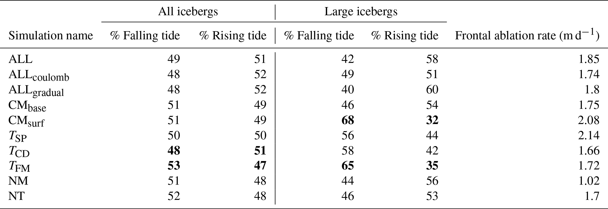
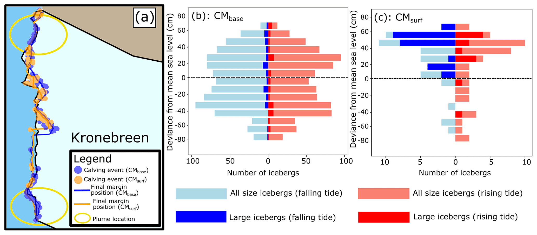
Figure 4Comparison of the results from CMbase and CMsurf. (a) Location of calving events in CMsurf (orange) and CMbase (blue) superimposed over the margin position from the beginning of the simulations (black), the end of CMsurf (orange), and the end of CMbase (blue). The locations of the plumes are indicated by the yellow ovals. (b, c) All size calving events (pale bars) and large calving events (dark bars) plotted with regards to the water depth at which they occurred, given in 10 cm intervals. The length of each bar denotes the number of icebergs occurring during each 10 cm water depth interval. Blue (red) bars indicate calving events on falling (rising) tide. Panel (b) shows results from CMbase, and panel (c) shows results from CMsurf, where significantly fewer calving events were modelled.
4.2 Impact of tides on calving
The occurrence of calving events from the simulations isolating tidal impacts (TSP, TFM, and TCD) during rising and falling tides is summarised in Table 2. When considering calvings of all sizes, TFM shows a statistically significant inclination to calve preferentially on a falling tide. In contrast, both TCD and TSP do not show a preference for any tidal phase. However, the large icebergs from all three simulations (corresponding to 5 % of the total icebergs) showed a preference for calving on a falling tide, with the TFM simulation showing the strongest and only statistically significant signal.
The relation between calving events and water depth (deviance from mean sea level) can reveal a more complex picture than can be garnered from considering the percentage of events occurring during different tidal phases. Instead, these data reveal if there is a relation between when calving occurs and absolute water levels (high or low) without consideration of the tidal phase. In Fig. 5c, data from TCD are shown. Close inspection of these results shows that large calving events in the TCD simulation tend to cluster around both high and low tides. No such relation was found between water depth and calving for the TSP and TFM simulations or for the TCD simulation and all size icebergs. The frontal ablation in all three simulations was similar, with a range of 0.48 m d−1. Additionally, the frontal ablation rate in these simulations was similar to that of the NT simulation, where no tidal fluctuations were included in the model set-up.
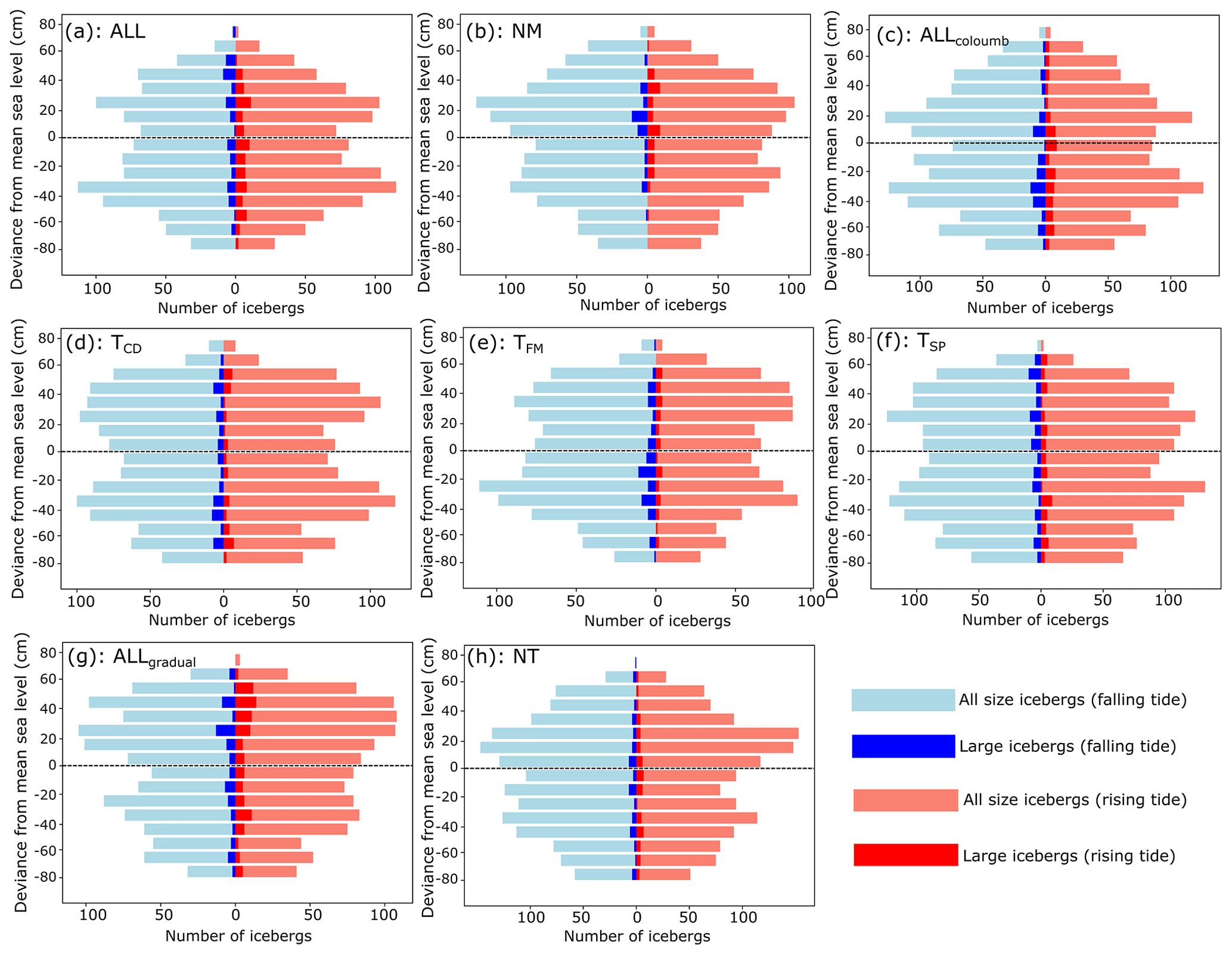
Figure 5All size calving events (pale bars) and large calving events (dark bars) plotted with regards to water depth (given in 10 cm intervals). The length of the line denotes the number of icebergs at a given 10 cm water depth interval. Blue bars denote that the calving event occurred on falling tide, and red bars denote the calving event occurred on a rising tide. Panel (a) shows results from ALL, panel (b) from NM, panel (c) from ALLcoulomb, panel (d) from TCD, panel (e) from TFM, panel (f) from TSP, panel (g) from ALLgradual, and panel (h) from NT.
4.3 Impacts of frontal melt and terminus geometry on calving
In the NM simulation, which is the only simulation without frontal melt included, a slight preference for calving on a falling tide is shown when considering all icebergs, and a larger preference is shown for calving on a rising tide when considering large icebergs (see Table 2 and Fig. 5). In terms of temporal trends, calving frequency is low in the first third of the simulation until 7 August, before picking up. Low calving frequencies are seen once more during the first neap tide (11 to 15 August), after which they increase again as the tidal amplitude increases.
This is in contrast to CMsurf, where a low calving frequency is seen throughout (Fig. 4). In addition, this is in contrast to all other simulations, where the general temporal trend is that calving frequency is initially high, after which a period of relative stability ensues. Around the middle of the simulation, calving activity picks up once again (an example from the TSP simulation is shown in Fig. 6). The NM simulation has some similarities to these other simulations but is distinct due the earlier onset of increased calving frequency and the correlation with tidal amplitude. The NM simulation has a lower frontal ablation rate than all the other simulations, likely at least in part due to the lack of frontal melt.
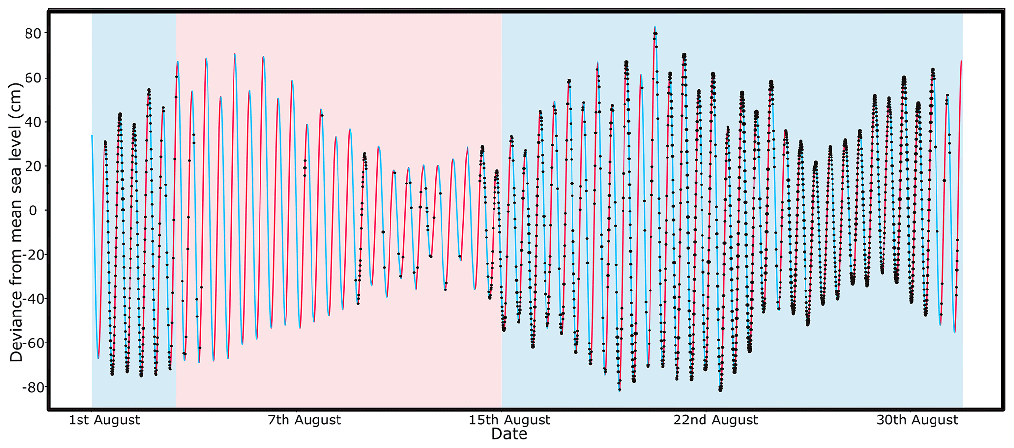
Figure 6Changes in water depth due to tides during August 2016, with rising tides shown as red lines and falling tides as blue lines. Calving events from the SP simulation are denoted by black dots. The blue shaded areas denotes the periods at the beginning of the simulation and between 15 and 31 August when calving activity is generally higher, whilst the red shaded areas denote lower calving frequencies. Neap tides can be seen between 11 and 15 August as well as between 26 and 30 August.
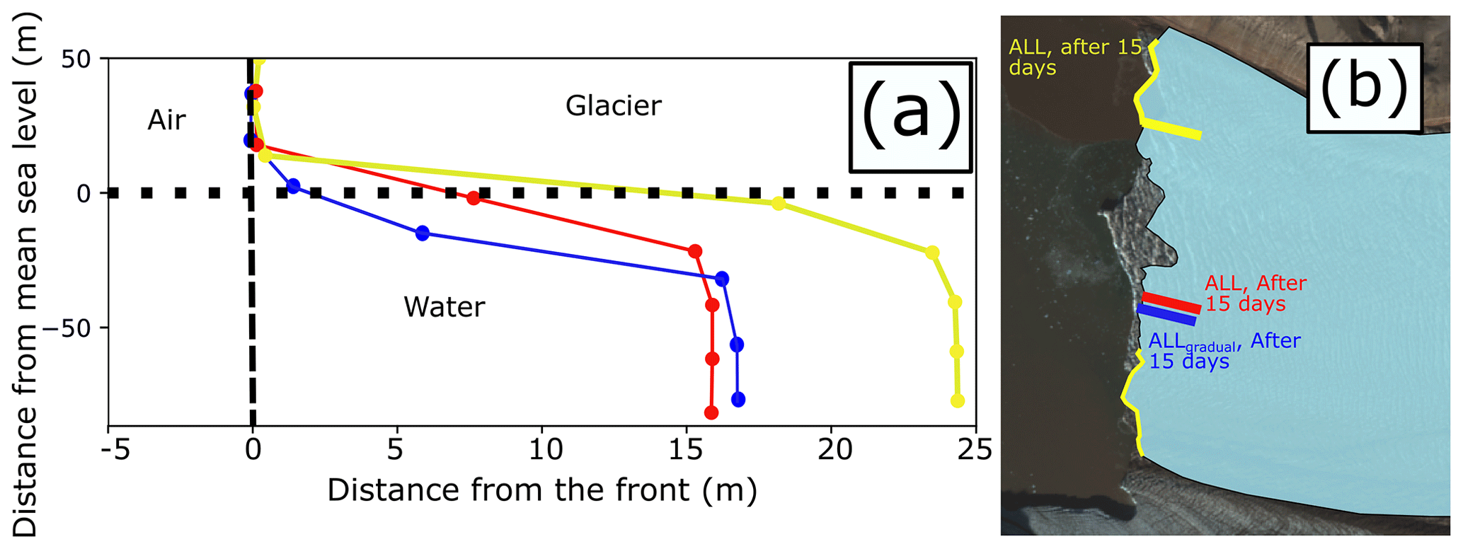
Figure 7(a) Undercut profiles from several simulations and locations normal to the orientation of the calving front of Kronebreen as denoted by the coloured lines and corresponding time labels in panel (b). The profiles show the modelled frontal morphology from 15 d into the ALL or ALLgradual simulation. The yellow profile corresponds to a plume location, and the red and blue profiles correspond to a non-plume location. The dotted black line denotes the mean water level, and the dashed black line denotes the front of the glaciers. (b) Modelled glacier outline from the midpoint of the simulation, with the location of the profiles (coloured lines) and plumes (yellow areas) shown. Background image: Copernicus Sentinel data (2022), retrieved from Copernicus Open Access Hub on 23 May 2022, processed by ESA.
The increase in calving frequency in all simulations except NM coincides with the development of a well-defined (ca. 20 m) melt-driven undercut at the terminus (cf. Fig. 7). The size of this modelled undercut varies throughout the simulations, with calving events leading to periodic reductions in size as part of the overhanging ice is removed. Modelled undercut sizes also vary spatially due to the differences in frontal melt rates across the calving front (Fig. 7). These spatial differences are also seen in the observational data, where an undercut of ca. 25 m is observed near a plume compared to only ca. 10 m in a non-plume area. The undercut size at which the modelled uptick in calving frequency occurs is similar in size to the ca. 25 m undercut seen in the green (X to X′) observational profile (see Fig. 2). This increase in calving activity was seen in the ALLgradual simulation, where a less angular undercut was modelled. However, the increase in frequency was more gradual and less well defined.
When focusing on the observed calving front morphology (Fig. 2), many small-scale geometries can be seen. In particular, both observed profiles show an undercut between the waterline and −20 m after which a straight front is seen. For the northern (orange) profile this straight front lasts for ca. 40 m whereas for the southern (green) profile this only lasts for ca. 10 m. Near the bottom of the ice cliff, both profiles show another undercut.
4.4 Impacts of sliding law on calving
The results from the Allcoulomb simulation can be compared to the results from the ALL simulation to understand the impact that sliding law choice has on calving dynamics in this model set-up. The number of icebergs occurring at each given water depth and on each tidal phase is shown in Fig. 5. Here, it can be seen that there is little difference between ALL and ALLcoulomb, with both simulations showing a relatively even amount of calving events on each tidal phase, with no statistically significant propensity to calve on a specific tidal phase. The total number of calving events was also similar for the two simulations. The frontal ablation rate was slightly lower in ALLcoulomb than ALL, but the difference was very small at 0.09 m d−1.
Additionally, both simulations showed the same temporal pattern of mainly low-frequency calving in the first half of the simulation, followed by high-frequency calving in the second half of the simulation (see Fig. 6 and Sect. 4.3).
The model results presented above provide insights into how the calving module in Elmer/Ice behaves and into which parameters the model is particularly sensitive to. However, as a result of both simplifications in the model set-up and general limitations of numerical models (detailed below), and despite the study being motivated by observational data from August 2016, the results should not be interpreted as a wholly accurate representation of calving at Kronebreen during August 2016. Notably, the model set-up did not prescribe any SMB during the course of the simulations.
5.1 Model limitations
Models are always an imperfect representation of reality, and there are several limitations of the model set-up used here which should be considered before inferences are made from the results.
Firstly, a viscous flow law not including purely elastic deformation was used to describe ice rheology. A viscous flow law of Glen type has been used in many modelling applications (e.g. Todd et al., 2018, 2019; Cook et al., 2020) and captures overall ice flow dynamics well. However, when approaching the calving front, material behaviour other than viscous may become important, too. For instance, both tidal cycles and individual calving events occur on short timescales and are, as such, related to both viscous and elastic deformation (e.g. Christmann et al., 2016, 2021; Reeh et al., 2003), raising the option to invoke a more complicated flow law than a purely viscous one. However, as the former will most certainly be computationally more expensive than the viscous flow law, improvements expected from using a better-suited flow law have to be seen in the context of the numerical experiments' feasibility and computational costs. Therefore, we here opted to run the simulations with a viscous flow law, as it allowed for a whole month of tidal cycles to be investigated which would not have been possible otherwise. However, this likely has some impact on the results, with previous work on a idealised geometry finding that larger and more frequent calving occurred when using an elastic model (Mosbeux et al., 2020).
Similarly, it can be asked why a continuous model is employed at a heavily crevassed and hence discontinuous glacier terminus, that could also be modelled with, for example, particle element modelling approaches (Åström et al., 2014; Prasanna et al., 2022). Elmer/Ice's Calving3D, however, also requests, by construction, a glacier with a heavily crevassed near-terminus region when employed, and where the yield strength required for fractures to initiate is ignored (Todd et al., 2018). However, crevasse advection from the upstream regions of the glacier towards the calving front is not taken into account, despite the fact that this process has been found to be important in certain situations (Berg and Bassis, 2022). Collectively, the choice of solvers, modules, and flow law made here implies that one should not necessarily expect reliable results at the scale of individual calving events but rather that the thousands of modelled calving events provide the opportunity to assess the broad patterns of calving behaviour and how this modelled behaviour may be impacted by, for example, tidal fluctuations.
Secondly, a rather simple melt parameterisation, kept constant during the course of the simulations, was chosen here as tidal cycles were the primary focus of this study. Notably, a simplified parameterisation of melt is likely to lead to undercut geometries which may not be representative of realistic ones and which, because of a distinct angular shape, may promote calving events as a result of unrealistically high stresses at the waterline. The model set-up also assumed that there was no melting or sublimation of the calving front above the waterline. Ignoring any such mass loss above the waterline may lead to an overestimation of undercut sizes, as in reality some melting of the calving front would also occur across the subaerial sections of the ice cliff, thus rendering the undercut less pronounced. Unfortunately, due to a lack of multibeam/lidar data from around the waterline, it is not clear what the terminus geometry of Kronebreen is like in reality. However, evidence from other glaciers suggests that a more gradual undercut is likely (Fried et al., 2015; Slater et al., 2021). The ALLgradual simulation provides some indication of the sensitivity of modelled calving events to undercut geometry and thus helps to negate some of the issues with the simple melt parameterisation. Furthermore, the impact of the angular geometry is the same regardless of whether the tide is rising or falling and so should have a limited impact on the results which relate calving activity to tidal phase.
Finally, notorious difficulties associated with representing processes in the inaccessible basal environment beneath a glacier would undoubtedly justify a more-in-depth analysis of the role of basal water pressure and spatio-temporal variations in basal friction (Vallot et al., 2018), as well as their representation in friction laws, on modelled results. While this is beyond the scope of the numerical experiments performed, a first indication of possible result sensitivity to the choice of sliding law can be obtained from comparing example simulations conducted with not only a Weertman-type sliding law, but also with a Coulomb-type one.
5.2 Calving mechanisms
When considering the CMsurf simulation, a clear preference is seen for large icebergs to be produced on a falling tide. When additionally taking into account the relationship between calving occurrence and absolute water depth (Fig. 4), it appears clear that calving in the CMsurf simulation preferentially occurs when water levels are higher. This makes sense; a higher water level makes it easier for the criterion of the “surf” calving mechanism to be satisfied. This relationship is not seen as clearly for the other simulations, but, in the majority of results, a bimodal distribution is seen in calving activity, with above-average water levels being associated with one of the peaks in calving activity. This suggests that there is some sensitivity in the model to water level, with higher water levels making it easier for the surface calving mechanism to be satisfied.
In contrast, the CMbase simulation shows a slight preference for large calvings on a rising tide, with this potentially being linked to increased buoyancy forces on a rising tide. However, this preference is not as clear as for other simulations and may well be an artefact of the model. Calving in CMbase is related to the propagation of both surface and basal crevasses, with calving activity particularly high in areas with plume melt (see Fig. 4a). This suggests that changes to the stress regime as a consequence of melt-driven undercutting may be of importance for modelled calving when considering the base calving mechanism.
5.3 Impacts of tides on calving
A preference for the calving of large icebergs during falling tide was shown in the TSP, TFM, and TCD simulations (Table 2, Sect. 4.2), with statistical significance only in the case of TFM (all size and large icebergs) and TCD (all size icebergs, with a preference for calving on a rising tide).
The relationship between the timing of calving in the TCD simulation and tidal phase is likely linked to the “surf” calving mechanism. Here, a high or rising tide reduces the distance that surface crevasses have to propagate to cause calving. The results displayed in Fig. 5d show that calving events tend to cluster around either high or low tides, which could point to different events being triggered by the two different calving mechanisms at play. Calving events which occur at high tide may be related to the propagation of surface crevasses, preferentially occurring when water levels are higher. However, the more numerous calving events occurring due to basal crevassing may instead preferentially occur at low tide and confuse the tidal signal. This clustering of calving events at low and high tide has been previously identified from observational data at Helheim Glacier, with the amount of water in crevasses and moulins being a potentially important factor for determining calving frequency (Vaňková and Holland, 2016). The influence of water level in surface crevasses in our simulations was not as strong as found in previous studies such as that by Cook et al. (2012), where the amount of water in surface crevasses was varied to look at the impact on calving. In Cook et al. (2012), the presence of increased water in crevasses led to a large increase in calving; an additional few metres of water caused the glacier to switch to a retreat of 1.9 km yr−1 from an advance of 3.5 km yr−1. It is important to note that this does not explicitly model tidal cycles but instead just considers the influence of water in crevasses.
It must also be noted that, in our model, water level in crevasses is assumed to be in equilibrium with tidal water level. Yet, it is possible that there is instead a delay in the connection between the fjord and crevasse water levels. This is an important factor to consider; a previous modelling study looking at calving found that crevasse opening is greatest at low tides (Van Dongen et al., 2020). However, this relationship is complex; it was the difference in water level between the crevasse and ocean that was most important, with maximum opening rates occurring when this difference was at least 4 m, as can occur when there is a delay in water drainage between the glacier and ocean (Van Dongen et al., 2020). Thus, further observational studies to determine how water levels in crevasses at Kronebreen vary are important for better constraining the influence of tides.
In the TFM simulation, a statistically significant preference to calve on a falling tide was seen – regardless of iceberg size. This is likely linked to undercut development, with the largest undercut sizes being seen on a falling tide as a result of accumulated frontal melt. The linkages between frontal melt, undercutting, and calving are discussed in more detail in Sect. 5.4.
In terms of TSP, no statistically significant relationship was found between calving and tidal phase. Previous research has found that a falling tide can promote calving by causing a reduction in the amount of back (sea) pressure exerted on the calving front. This mechanism has been documented at Tunabreen, Svalbard, where How et al. (2019) conducted a time lapse study and found that 68 % of calving events occurred on a falling tide. Changes in the water level during the study period led to a 2 % reduction in back stress during low tide, with this small change being sufficient to cause increased numbers of calving events. Another observational study found similar results, with large calvings at Yahtse Glacier, Alaska, being significantly more likely during low or falling tides than during high or rising tides – but with this impact only being clear for large icebergs (Bartholomaus et al., 2015). Additional studies have also linked changes in back pressure to velocity variations, with peaks in velocity associated with low tide as well as variations in ice mélange back pressure (Voytenko et al., 2015). However, whilst modelled changes in back pressure have an impact on the terminus stress regime and thus crevasse propagation, our results presented here do not suggest a sensitivity to this. As such, we are unable to demonstrate the strong linkage between changing back stress and calving that is suggested from observational studies at other glaciers. Site-specific conditions at Kronebreen could be partly responsible, but this remains speculative. The lack of correlation is likely partly a result of the absence of elastic strain in the model set-up used for this study. This is due to the fact that changes in stress regime as a result of changes in the exertion of sea pressure over a tidal cycle are transmitted too slowly by the purely viscous model used here to have an impact on crevasse propagation and, as such, calving.
5.4 Impacts of frontal melt and terminus geometry on calving
The results presented in Sect. 4.3 show that the development of a melt-driven undercut is associated with an increase in the calving frequency in all simulations except CMbase and NM, highlighting the role terminus geometry plays in glacier tidal response.
Previous modelling work at Store glacier, Greenland, found that basal crevasse propagation was much higher across parts of the glacier front which were floating (Todd et al., 2018). In this study, also conducted using the Calving3D module in Elmer/Ice, buoyancy forces acting on the floating parts of the terminus were seen to promote basal crevassing and subsequent calving. This often occurred in conjunction with changes in the stress regime as precipitated by melt undercutting (Todd et al., 2018). This links to the TFM simulation, where the proposed mechanism for more frequent calving on the falling tide is that frontal melt accumulates during both the rising and falling tides, leading to the largest undercuts occurring during the falling tide. When the undercuts are largest, basal crevasses are able to propagate due to higher basal water pressures and so can lead to increased calving on a falling tide (Todd et al., 2018). Given that large calving events from the TFM simulation showed one of the strongest tidal signals, combined with the fact that all size calving and large calving statistics from TFM were significant, it appears that melt-driven undercutting has a particularly strong impact on calving patterns in the model.
In this model set-up, we propose that a similar mechanism to that described by Todd et al. (2018) for Store glacier is at play. At Kronebreen, the development of a well-defined undercut of around 20 m is suggested to lead to accelerated basal crevassing and calving. Evidence for this comes from the fact that the calving frequency in all of the simulations except for CMsurf and NM increases in the latter half of the simulation once the undercut has reached this critical size. In addition, calving during the CMbase simulation increasingly clusters around plume locations as time goes on, where the modelled undercuts are largest (Fig. 6 and Sect. 4.1). A greater proportion of calving events occurring due to basal crevasse propagation were considered small than events occurring from surface crevasse propagation. This suggests that the smaller, more frequent calving events in the model of Kronebreen are primarily controlled by undercut development and may be independent of tidal fluctuations.
The temporal pattern of increased calving around the midpoint of the simulations was additionally seen in the ALLgradual simulation, but here it was less defined and the onset of higher calving frequencies occurred more gradually than in other scenarios. This suggests that, as a result of the angular undercuts in the majority of the simulations, the temporal patterns displayed by the model are likely exaggerated.
In the absence of any frontal melt, the NM simulation shows increased large iceberg calving during rising tides. We suggest that, in the absence of an undercut, calving events in the model are predominantly caused by surface crevasse propagation. In this scenario, a high or rising water level makes it easier for these surface crevasses to reach the waterline. There is also some indication that tidal amplitude is important for calving in NM, as calving frequency drops during the first neap tide before picking back up again as the tidal amplitude increases (see Sect. 4.3 and tidal cycles in Fig. 6). This could be due to the fact that, when tidal amplitudes are higher, the distance that a surface crevasse must propagate to reach water level is at a minimum. However, during the second neap tide the reduction in calving frequency is less defined, suggesting a complex relationship. This type of nuanced pattern has some basis in reality; observations at LeConte glacier, Alaska, suggested that calving was correlated to the amplitude of tidal cycles (O'Neel et al., 2003). As with our model data, evidence was found for increased calving during spring tides (O'Neel et al., 2003).
The development of a ca. 20 m undercut was a key determinant of calving frequency in the model, raising the question of how well the modelled undercut geometry corresponds to observations. Consideration of the observed profiles of Kronebreen's frontal geometry (Fig. 2) shows that the calving front morphology is, in reality, much more complex than that achieved by our simple melt parameterisation. The presence of an undercut just below the waterline at around −20 m is likely due to warm waters, with sound velocity profiles presented by Holmes et al. (2019) showing that the warmest waters (ca. 6 ∘C) during mid August 2016 were located at or around a depth of 20 m. The undercuts near the base of the profiles are instead likely a consequence of sub-glacial discharge, with a more pronounced undercut on the southern (green) profile where a subglacial plume can be identified on satellite imagery. Incorporation of these more nuanced frontal melt patterns would be beneficial for further understanding the controls on calving at Kronebreen and for running simulations to investigate the impact of calving events of glacier dynamics similarly to e.g. Amundson et al. (2022). This is particularly important because a small change to the terminus geometry (as in the ALLgradual simulation) can alter the temporal patterns in calving seen in the model results. The lack of data from the 20 m section under the waterline hinders evaluation of undercut geometry, but future studies which include the use of uncrewed vehicles that can get closer to the calving front will likely allow a greater proportion of the ice cliff to be imaged.
In terms of undercut magnitude, the observational MB/lidar data show that undercut size at Kronebreen can be around 25 m at plume locations and around 10 m at non-plume locations (see Fig. 2). The modelled plume undercut at the midpoint of the simulations corresponds well to the size of the observed plume undercut, with this being the time point at which calving frequency tends to increase in the model (Fig. 7). At non-plume locations, the model overestimates undercut size (17.5 m compared to 10 m). However, the observations only show two in situ profiles – it is thus not clear how variable the undercut size can be, either temporally or spatially. Previous studies have found evidence for large spatial variability in undercut sizes at other glaciers, making it likely that the same holds true for Kronebreen (Fried et al., 2015; Rignot et al., 2015). The modelled undercut reaches a mean of ca. 40 m in size by the end of the simulations, which is likely larger than reality. However, we do not observe any further changes in calving patterns as the undercut continues to grow.
Our modelled undercuts are generally smaller than those modelled by Vallot et al. (2018). There, undercuts at Kronebreen were also modelled using Elmer/Ice, and sizes of up to ca. 150 m were found for a high-discharge plume area and up to ca. 40 m for a low-discharge plume area (Vallot et al., 2018). However, Vallot et al. (2018) note that the undercuts were allowed to develop with no calving implemented, which likely makes them overestimates. Further work is thus needed to better understand the frontal morphology of Kronebreen and its impacts for calving patterns. Despite this, both the observational and model data presented here suggest that frontal melt is significant at Kronebreen, agreeing with previous studies and adding weight to the argument that frontal melt exerts a first-order control on its calving dynamics (Luckman et al., 2015; Holmes et al., 2019). In addition, the results presented here provide evidence for terminus geometry being an important modulator of calving behaviour and suggest that future modelling experiments should include realistic terminus geometries, where observational data are available to guide this.
5.5 Impacts of sliding law on calving
Very little difference was found between the results from simulations ALL and ALLcoulomb, with an approximately even split between calving events on each tidal phase, and similar frontal ablation rates and temporal trends in calving frequency.
This suggests that the modelled calving patterns are not particularly sensitive to the sliding law used. This could be partly due to the timescale of the simulations, with 1 month being too short for clear differences to be identified. Yet, the short timescale helps to reduce any errors associated with the Weertman friction law and the high variability of basal friction at Kronebreen (Vallot et al., 2017). Previous studies have highlighted the importance of effective pressure for tidal response, leading to an expectation that the differences between the Weertman and Coulomb simulations should be larger (Waiters and Survey, 1989; Amundson et al., 2022). However, there is also evidence that there are certain regimes where the effect of tides on effective pressure is small, and that could be the case here (Amundson et al., 2022). Conducting longer-term simulations with different sliding laws and, additionally, SMB forcing included to allow for thinning of the ice cliff not modelled here will help elucidate further how sensitive model results are to the choice of basal conditions.
5.6 Frontal ablation rates
Modelled and observed frontal ablation rates can be compared to give an indication on whether the model is able to reproduce general glacier behaviour. Frontal ablation rates at Kronebreen have been previously calculated for various years and show a degree of temporal variation. For 2013 and 2014, Luckman et al. (2015) found summertime frontal ablation rates of between 4 and 8 m d−1. For the summers of 2016 and 2017, lower frontal ablation rates of between 2–7 m d−1 were found by Holmes et al. (2019). In this modelling study, the lowest frontal ablation rates were found in the NM simulation, at around 1 m d−1, with the rest of the simulations showing frontal ablation rates of between 1.66 and 2.14 m d−1. This is lower than observationally derived estimates of frontal ablation rates, likely as a result of the simple melt rate parameterisation (which is lower than some observationally derived estimates of submarine melt rates) or as a result of the lack of SMB forcing (Köhler et al., 2019). Further, the frontal ablation rate from the NT simulation was similar to other simulations, suggesting that even if the timing of calving events is impacted by tidal cycles, their inclusion in models is unlikely to lead to changes in bulk frontal ablation rates.
Tidal impacts on modelled calving at Kronebreen are complex, with a clear relationship only being seen when certain calving mechanisms or tidal impacts are considered. High water levels are seen to promote calving in the model by reducing the depth to which surface crevasses must propagate. However, the development of a melt-derived undercut of ca. 20 m leads to the increased propagation of basal crevasses and an increased frequency of calving events which do not show a tidal signal. This suggests that, when undercuts in the model reach a critical size, their presence exerts a first-order control on modelled calving. During these periods, tidal fluctuations constitute only a second-order control on calving dynamics.
These findings suggest that frontal melt may be of great importance for calving at Kronebreen and provide motivation for investigating model sensitivity to spatio-temporal variations in undercut sizes. Similarly, further modelling experiments which utilise more realistic frontal melt scenarios and undercut geometries, incorporate more investigation of sliding law choice, and look into the longer-term development of Kronebreen would constitute useful future modelling experiments.
A1 Results related to stages I to III, from inversion for basal friction to relaxed, spun-up state of Kronebreen
The Robin inverse method aims to minimise a cost function that measures the mismatch between modelled and observed velocities and is described in more detail by, for example, Gillet-Chaulet et al. (2012). A regularisation parameter, λ, is tuned in order to find the best compromise between the smoothness of the inverted field and the minimisation of the cost function. The parameter λ is chosen by creating an L curve (Fig. A1) and choosing the value at the base of the L (Hansen, 2001). The L-curve plots Jreg (smoothness of the inverted field) against JO (mismatch between the model and observations). The chosen value of λ in this study, 5.0×10⁹, ensures that the misfit between the modelled and observed velocities remains small whilst not causing too much smoothing of the basal friction field. The inverted summer basal friction field used for the suite of main simulations is shown in Fig. A2a. Here, lower friction values can be seen across the southern edge of Kronebreen, which is a similar pattern to that found by Vallot et al. (2018) during summer 2013.
The modelled summer velocities at the end of stage I (inversion) are shown in Fig. A2b, with frontal velocities reaching up to 750 m yr−1 (2.05 m d−1). This corresponds well to observed velocities from the summer of 2016, where mean frontal velocities reached highs of ca. 2 m d−1 (Holmes et al., 2019). At the end of stage II (spin-up), velocities show a similar maximum magnitude but extend over a greater proportion of the terminus area (see Fig. A2c). The mean frontal velocities from the area denoted by the black polygon in Fig. A2c are shown in Fig. A3. Note that, even in a steady state, seasonal variations in velocity are seen as a result of varying temperature forcing and basal friction (Fig. A3). The position of the calving front changes during stage III (relaxation), with the change in frontal and surface geometries occurring synchronously with a slowdown in velocity (Fig. A2d). The frontal velocities instead lie around 1.8–1.9 m d−1, which remains within the range of summer 2016 velocities observed at Kronebreen (Holmes et al., 2019). The results shown in Fig. A2d correspond to the initial conditions for all simulations in stage IV.
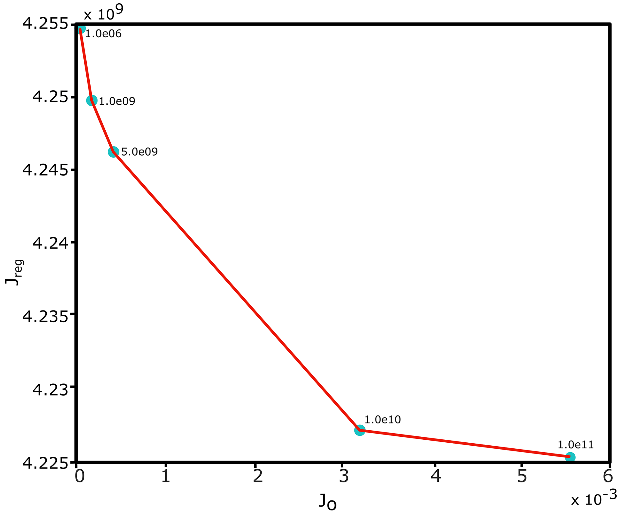
Figure A1L curve from the summer inversion, with the λ values shown next to the data points. The chosen value for λ is 5.0×10⁹. The x axis shows JO (mismatch between the model and observations), and the y axis shows Jreg (variable smoothness).
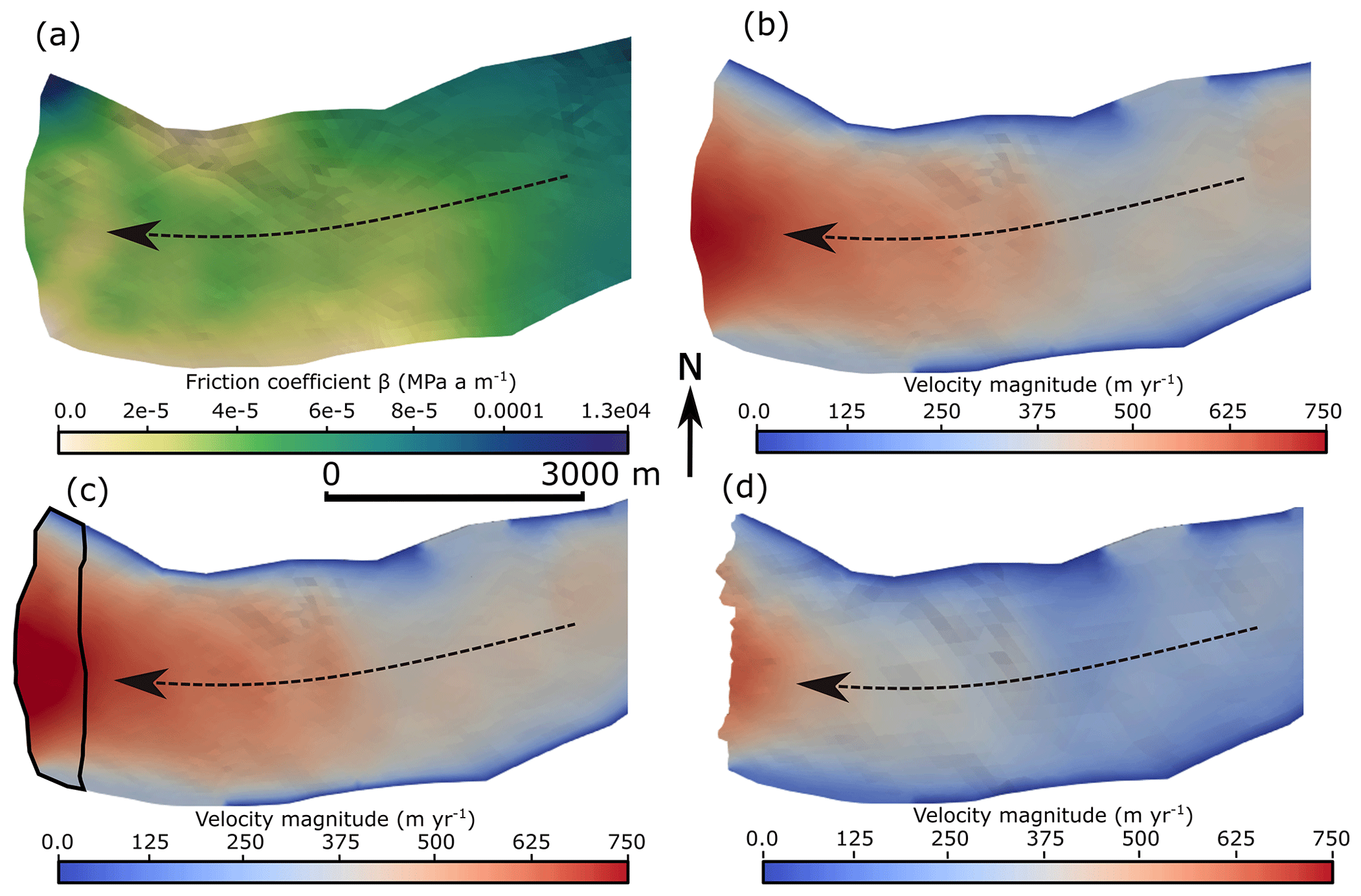
Figure A2Results from steps I to III of the simulation workflow for the frontal portion of Kronebreen. In all panels, the dotted lines shown the flow direction. (a) Inverted summer basal friction at Kronebreen. (b) Modelled summer velocities at Kronebreen at the end of stage I (inversion). (c) Modelled summer velocities at Kronebreen at the end of stage II (spin-up), with the black polygon denoting the area over which mean velocity values were calculated for plotting in Fig. A3. (d) Modelled summer velocities and margin position at the end of stage II (relaxation).
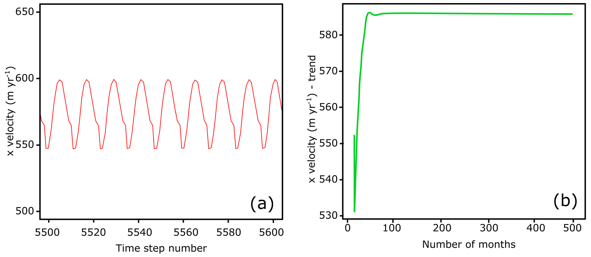
Figure A3Example results from the spin-up showing mean frontal velocities in the x direction (positive denoting flow towards the glacier terminus). The frontal area from where mean velocities are calculated is shown by the black polygon in Fig. A2c. (a) A close-up of the x-velocity time series from the spin-up simulation, with clear seasonal variation visible. The nine peaks in the figure correspond to nine subsequent summer velocity maxima. (b) The decomposed trend of the x velocities from the spin-up. By the end of the spin-up, there is no directional trend, thus showing the velocities to have converged.
The code for the Elmer/Ice model is available at https://github.com/ElmerCSC/elmerfem (Gagliardini et al., 2013). The multibeam and lidar data used for the frontal profile of Kronebreen are available from the Bolin Centre for Climate Research's database (https://doi.org/10.17043/noormets-2022-kronebreen-1, Noormets et al., 2022). The tidal data used are available from https://kartverket.no (Norwegian Mapping Authority, 2022). The SMB data used for the model spin-up are available online at https://doi.org/10.1594/PANGAEA.920984 (Noël et al., 2020).
FAH designed the study, with the help of NK and EvD. FAH ran the simulations with assistance from EvD and NK. The multibeam data were collected by RN and NK, and the lidar data were collected by MP. FAH and NK wrote the manuscript, with the help of all authors.
The contact author has declared that none of the authors has any competing interests.
Publisher’s note: Copernicus Publications remains neutral with regard to jurisdictional claims in published maps and institutional affiliations.
The lidar and multibeam data were collected as part of the CalvingSEIS project, funded by the Research Council of Norway. The authors are grateful to Brice Noël for the daily SMB data used in the model spin-up. MP received support from the Anthropocene Priority Research Area under the Strategic Programme Excellence Initiative at the Jagiellonian University. We are grateful to the editor, Ben Marzeion, as well as Jason Amundson, Douglas Benn, Jeremy Bassis, and one anonymous reviewer for their insightful comments on earlier versions of the manuscript.
This research has been supported by the Svenska Forskningsrådet Formas (grant nos. 214-2013-1600 and 2017-00665).
The article processing charges for this open-access publication were covered by Stockholm University.
This paper was edited by Ben Marzeion and reviewed by Jason Amundson, Jeremy Bassis, Douglas Benn, and one anonymous referee.
Amundson, J. M., Truffer, M., and Zwinger, T.: Tidewater glacier response to individual calving events, J. Glaciol., 68, 1117–1126, https://doi.org/10.1017/JOG.2022.26, 2022. a, b, c, d
Arthern, R. J. and Gudmundsson, G. H.: Initialization of ice-sheet forecasts viewed as an inverse Robin problem, J. Glaciol., 56, 527–533, https://doi.org/10.3189/002214310792447699, 2010. a
Åström, J. A., Vallot, D., Schäfer, M., Welty, E. Z., O’Neel, S., Bartholomaus, T. C., Liu, Y., Riikilä, T. I., Zwinger, T., Timonen, J., and Moore, J. C.: Termini of calving glaciers as self-organized critical systems, Nat. Geosci., 7, 874–878, https://doi.org/10.1038/ngeo2290, 2014. a
Bartholomaus, T. C., Larsen, C. F., West, M. E., O'Neel, S., Pettit, E. C., and Truffer, M.: Tidal and seasonal variations in calving flux observed with passive seismology, J. Geophys. Res.-Earth, 120, 2318–2337, https://doi.org/10.1002/2015JF003641, 2015. a, b
Benn, D. I., Warren, C. R., and Mottram, R. H.: Calving processes and the dynamics of calving glaciers, Earth-Sci. Rev., 82, 143–179, https://doi.org/10.1016/J.EARSCIREV.2007.02.002, 2007. a, b
Berg, B. and Bassis, J.: Crevasse advection increases glacier calving, J. Glaciol., 68, 977–986, https://doi.org/10.1017/JOG.2022.10, 2022. a
Błaszczyk, M., Jania, J., and Res, J. H.: Tidewater glaciers of Svalbard: Recent changes and estimates of calving fluxes, Pol. Polar Res., 30, 85–142, https://journals.pan.pl/dlibra/publication/126668/edition/110542/content (last access: 2 May 2023), 2009. a
Braun, M., Pohjola, V. A., Pettersson, R., Möller, M., Finkelnburg, R., Falk, U., Scherer, D., and Schneider, C.: Changes of glacier frontal positions of vestfonna (nordaustlandet, svalbard), Geogr. Ann. A, 93, 301–310, https://doi.org/10.1111/J.1468-0459.2011.00437.X, 2016. a
Christmann, J., Plate, C., Müller, R., and Humbert, A.: Viscous and viscoelastic stress states at the calving front of Antarctic ice shelves, Ann. Glaciol., 57, 10–18, https://doi.org/10.1017/AOG.2016.18, 2016. a
Christmann, J., Helm, V., Khan, S. A., Kleiner, T., Müller, R., Morlighem, M., Neckel, N., Rückamp, M., Steinhage, D., Zeising, O., and Humbert, A.: Elastic deformation plays a non-negligible role in Greenland’s outlet glacier flow, Communications Earth & Environment 2, 1–12, https://doi.org/10.1038/s43247-021-00296-3, 2021. a
Christoffersen, P., Mugford, R. I., Heywood, K. J., Joughin, I., Dowdeswell, J. A., Syvitski, J. P. M., Luckman, A., and Benham, T. J.: Warming of waters in an East Greenland fjord prior to glacier retreat: mechanisms and connection to large-scale atmospheric conditions, The Cryosphere, 5, 701–714, https://doi.org/10.5194/tc-5-701-2011, 2011. a, b
Cokelet, E. D., Tervalon, N., and Bellingham, J. G.: Hydrography of the West Spitsbergen Current, Svalbard Branch: Autumn 2001, J. Geophys. Res., 113, C01006, https://doi.org/10.1029/2007JC004150, 2008. a
Cook, S., Zwinger, T., Rutt, I. C., O'Neel, S., and Murray, T.: Testing the effect of water in crevasses on a physically based calving model, Ann. Glaciol., 53, 90–96, https://doi.org/10.3189/2012AOG60A107, 2012. a, b
Cook, S. J., Christoffersen, P., Todd, J., Slater, D., and Chauché, N.: Coupled modelling of subglacial hydrology and calving-front melting at Store Glacier, West Greenland , The Cryosphere, 14, 905–924, https://doi.org/10.5194/tc-14-905-2020, 2020. a, b
Cottier, F., Tverberg, V., Inall, M., Svendsen, H., Nilsen, F., and Griffiths, C.: Water mass modification in an Arctic fjord through cross-shelf exchange: The seasonal hydrography of Kongsfjorden, Svalbard, J. Geophys. Res., 110, C12005, https://doi.org/10.1029/2004JC002757, 2005. a
Deschamps-Berger, C., Nuth, C., Van Pelt, W., Berthier, E., Kohler, J., and Altena, B.: Closing the mass budget of a tidewater glacier: the example of Kronebreen, Svalbard, J. Glaciol., 65, 136–148, https://doi.org/10.1017/JOG.2018.98, 2019. a
Dunse, T., Schuler, T. V., Hagen, J. O., and Reijmer, C. H.: Seasonal speed-up of two outlet glaciers of Austfonna, Svalbard, inferred from continuous GPS measurements, The Cryosphere, 6, 453–466, https://doi.org/10.5194/tc-6-453-2012, 2012. a
Enderlin, E. M., Howat, I. M., Jeong, S., Noh, M. J., Van Angelen, J. H., and Van Den Broeke, M. R.: An improved mass budget for the Greenland ice sheet, Geophys. Res. Lett., 41, 866–872, https://doi.org/10.1002/2013GL059010, 2014. a
Fried, M. J., Catania, G. A., Bartholomaus, T. C., Duncan, D., Davis, M., Stearns, L. A., Nash, J., Shroyer, E., and Sutherland, D.: Distributed subglacial discharge drives significant submarine melt at a Greenland tidewater glacier, Geophys. Res. Lett., 42, 9328–9336, https://doi.org/10.1002/2015GL065806, 2015. a, b
Gagliardini, O., Cohen, D., Råback, P., and Zwinger, T.: Finite-element modeling of subglacial cavities and related friction law, J. Geophys. Res.-Earth, 112, 2027, https://doi.org/10.1029/2006JF000576, 2007. a
Gagliardini, O., Zwinger, T., Gillet-Chaulet, F., Durand, G., Favier, L., de Fleurian, B., Greve, R., Malinen, M., Martín, C., Råback, P., Ruokolainen, J., Sacchettini, M., Schäfer, M., Seddik, H., and Thies, J.: Capabilities and performance of Elmer/Ice, a new-generation ice sheet model, Geosci. Model Dev., 6, 1299–1318, https://doi.org/10.5194/gmd-6-1299-2013, 2013 (code available at: https://github.com/ElmerCSC/elmerfem, last access: February 2022). a, b
Gillet-Chaulet, F., Gagliardini, O., Seddik, H., Nodet, M., Durand, G., Ritz, C., Zwinger, T., Greve, R., and Vaughan, D. G.: Greenland ice sheet contribution to sea-level rise from a new-generation ice-sheet model, The Cryosphere, 6, 1561–1576, https://doi.org/10.5194/tc-6-1561-2012, 2012. a, b
Hansen, P. C.: The L-curve and its use in the numerical treatment of inverse problems, in: Computational inverse problems in electrocardiology, WIT Press, 119–142, ISBN 978-1-85312-614-7, 2001. a
Holland, D. M., Thomas, R. H., de Young, B., Ribergaard, M. H., and Lyberth, B.: Acceleration of Jakobshavn Isbræ triggered by warm subsurface ocean waters, Nat. Geosci., 1, 659–664, https://doi.org/10.1038/ngeo316, 2008. a
Holmes, F. A., Kirchner, N., Kuttenkeuler, J., Krützfeldt, J., and Noormets, R.: Relating ocean temperatures to frontal ablation rates at Svalbard tidewater glaciers: Insights from glacier proximal datasets, Scientific Reports, 9, 9442, https://doi.org/10.1038/s41598-019-45077-3, 2019. a, b, c, d, e, f, g, h, i, j
Holmes, F. A., Kirchner, N., Prakash, A., Stranne, C., Dijkstra, S., and Jakobsson, M.: Calving at Ryder Glacier, Northern Greenland, J. Geophys. Res.-Earth, 126, e2020JF005872, https://doi.org/10.1029/2020JF005872, 2021. a
How, P., Schild, K. M., Benn, D. I., Noormets, R., Kirchner, N., Luckman, A., Vallot, D., Hulton, N. R. J., and Borstad, C.: Calving controlled by melt-under-cutting: detailed calving styles revealed through time-lapse observations, Ann. Glaciol., 60, 20–31, https://doi.org/10.1017/aog.2018.28, 2019. a, b
IPCC: IPCC Special Report on the Ocean and Cryosphere in a Changing Climate, Intergovernmental Panel on Climate Change, Cambridge University Press, ISBN 9781009157964, https://doi.org/10.1017/9781009157964, 2022. a
Jakobsson, M., Mayer, L. A., Nilsson, J., Stranne, C., Calder, B., O’Regan, M., Farrell, J. W., Cronin, T. M., Brüchert, V., Chawarski, J., Eriksson, B., Fredriksson, J., Gemery, L., Glueder, A., Holmes, F. A., Jerram, K., Kirchner, N., Mix, A., Muchowski, J., Prakash, A., Reilly, B., Thornton, B., Ulfsbo, A., Weidner, E., Åkesson, H., Handl, T., Ståhl, E., Boze, L.-G., Reed, S., West, G., and Padman, J.: Ryder Glacier in northwest Greenland is shielded from warm Atlantic water by a bathymetric sill, Communications Earth & Environment, 1, 45, https://doi.org/10.1038/s43247-020-00043-0, 2020. a
Jenkins, A.: Convection-Driven Melting near the Grounding Lines of Ice Shelves and Tidewater Glaciers, J. Phys. Oceanogr., 41, 2279–2294, https://doi.org/10.1175/JPO-D-11-03.1, 2011. a
Joughin, I., Smith, B. E., and Schoof, C. G.: Regularized Coulomb Friction Laws for Ice Sheet Sliding: Application to Pine Island Glacier, Antarctica, Geophys. Res. Lett., 46, 4764–4771, https://doi.org/10.1029/2019GL082526, 2019. a
Karlsson, N. B., Solgaard, A. M., Mankoff, K. D., Gillet-Chaulet, F., MacGregor, J. A., Box, J. E., Citterio, M., Colgan, W. T., Larsen, S. H., Kjeldsen, K. K., Korsgaard, N. J., Benn, D. I., Hewitt, I. J., and Fausto, R. S.: A first constraint on basal melt-water production of the Greenland ice sheet, Nat. Commun., 12, 3461, https://doi.org/10.1038/s41467-021-23739-z, 2021. a
King, M. D., Howat, I. M., Candela, S. G., Noh, M. J., Jeong, S., Noël, B. P. Y., van den Broeke, M. R., Wouters, B., and Negrete, A.: Dynamic ice loss from the Greenland Ice Sheet driven by sustained glacier retreat, Communications Earth & Environment, 1, 1, https://doi.org/10.1038/s43247-020-0001-2, 2020. a, b
Köhler, A., Pętlicki, M., Lefeuvre, P.-M., Buscaino, G., Nuth, C., and Weidle, C.: Contribution of calving to frontal ablation quantified from seismic and hydroacoustic observations calibrated with lidar volume measurements, The Cryosphere, 13, 3117–3137, https://doi.org/10.5194/tc-13-3117-2019, 2019. a, b
Le clec'h, S., Quiquet, A., Charbit, S., Dumas, C., Kageyama, M., and Ritz, C.: A rapidly converging initialisation method to simulate the present-day Greenland ice sheet using the GRISLI ice sheet model (version 1.3), Geosci. Model Dev., 12, 2481–2499, https://doi.org/10.5194/gmd-12-2481-2019, 2019. a
Lindbäck, K., Kohler, J., Pettersson, R., Nuth, C., Langley, K., Messerli, A., Vallot, D., Matsuoka, K., and Brandt, O.: Subglacial topography, ice thickness, and bathymetry of Kongsfjorden, northwestern Svalbard, Earth Syst. Sci. Data, 10, 1769–1781, https://doi.org/10.5194/essd-10-1769-2018, 2018. a
Luckman, A., Benn, D. I., Cottier, F., Bevan, S., Nilsen, F., and Inall, M.: Calving rates at tidewater glaciers vary strongly with ocean temperature, Nat. Commun., 6, 8566, https://doi.org/10.1038/ncomms9566, 2015. a, b, c, d, e
Mosbeux, C., Wagner, T. J., Becker, M. K., and Fricker, H. A.: Viscous and elastic buoyancy stresses as drivers of ice-shelf calving, J. Glaciol., 66, 643–657, https://doi.org/10.1017/JOG.2020.35, 2020. a
Nilsen, F., Cottier, F., Skogseth, R., and Mattsson, S.: Fjord-shelf exchanges controlled by ice and brine production: The interannual variation of Atlantic Water in Isfjorden, Svalbard, Cont. Shelf Res., 28, 1838–1853, https://doi.org/10.1016/J.CSR.2008.04.015, 2008. a
Noël, B. P. Y., Jakobs, C. L., van Pelt, W., Lhermitte, S., Wouters, B., Kohler, J., Hagen, J. O., Luks, B., Reijmer, C., van de Berg, W. J., and van den Broeke, M. R.: Annual surface mass balance (SMB) and components of Svalbard glaciers statistically downscaled to 500 m spatial resolution (1958–2018), PANGAEA [data set], https://doi.org/10.1594/PANGAEA.920984, 2020. a, b
Noormets, R., Pętlicki, M., and Kirchner, N.: Subaerial and submarine frontal morphology of Kronebreen, Svalbard, 24 August 2016, Bolin Centre Database [data set], https://doi.org/10.17043/noormets-2022-kronebreen-1, 2022. a
Norwegian Mapping Authority: Homepage, https://kartverket.no, last access: February 2022. a
O'Neel, S., Echelmeyer, K. A., and Motyka, R. J.: Short-term variations in calving of a tidewater glacier: LeConte Glacier, Alaska, U.S.A., J. Glaciol., 49, 587–598, https://doi.org/10.3189/172756503781830430, 2003. a, b
Podrasky, D., Truffer, M., Lüthi, M., and Fahnestock, M.: Quantifying velocity response to ocean tides and calving near the terminus of Jakobshavn Isbræ, Greenland, J. Glaciol., 60, 609–621, https://doi.org/10.3189/2014JOG13J130, 2014. a
Prasanna, M., Polojärvi, A., Wei, M., and Åström, J.: Modeling ice block failure within drift ice and ice rubble, Phys. Rev. E, 105, 045001, https://doi.org/10.1103/PHYSREVE.105.045001, 2022. a
Price, S. F., Payne, A. J., Howat, I. M., and Smith, B. E.: Committed sea-level rise for the next century from Greenland ice sheet dynamics during the past decade., P. Natl. Acad. Sci. USA, 108, 8978–83, https://doi.org/10.1073/pnas.1017313108, 2011. a
Promińska, A., Cisek, M., and Walczowski, W.: Kongsfjorden and Hornsund hydrography – comparative study based on a multiyear survey in fjords of west Spitsbergen, Oceanologia, 59, 397–412, https://doi.org/10.1016/J.OCEANO.2017.07.003, 2017. a
Reeh, N., Christensen, E. L., Mayer, C., and Olesen, O. B.: Tidal bending of glaciers: a linear viscoelastic approach, Ann. Glaciol., 37, 83–89, https://doi.org/10.3189/172756403781815663, 2003. a
Rignot, E. and Kanagaratnam, P.: Changes in the Velocity Structure of the Greenland Ice Sheet, Science, 311, 986–990, https://doi.org/10.1126/SCIENCE.1121381, 2006. a
Rignot, E., Fenty, I., Xu, Y., Cai, C., and Kemp, C.: Undercutting of marine-terminating glaciers in West Greenland, Geophys. Res. Lett., 42, 5909–5917, https://doi.org/10.1002/2015GL064236, 2015. a
Sato, T. and Greve, R.: Sensitivity experiments for the Antarctic ice sheet with varied sub-ice-shelf melting rates, Ann. Glaciol., 53, 221–228, https://doi.org/10.3189/2012AOG60A042, 2012. a
Schellenberger, T., Dunse, T., Kääb, A., Kohler, J., and Reijmer, C. H.: Surface speed and frontal ablation of Kronebreen and Kongsbreen, NW Svalbard, from SAR offset tracking, The Cryosphere, 9, 2339–2355, https://doi.org/10.5194/tc-9-2339-2015, 2015. a, b, c
Schoof, C.: The effect of cavitation on glacier sliding, P. Roy. Soc. A-Math. Phy., 461, 609–627, https://doi.org/10.1098/RSPA.2004.1350, 2005. a
Schuler, T. V., Kohler, J., Elagina, N., Hagen, J. O. M., Hodson, A. J., Jania, J. A., Kääb, A. M., Luks, B., Małecki, J., Moholdt, G., Pohjola, V. A., Sobota, I., and Van Pelt, W. J.: Reconciling Svalbard Glacier Mass Balance, Front. Earth Sci., 8, https://doi.org/10.3389/feart.2020.00156, 2020. a, b
Seddik, H., Greve, R., Zwinger, T., Gillet-Chaulet, F., and Gagliardini, O.: Simulations of the Greenland ice sheet 100 years into the future with the full Stokes model Elmer/Ice, J. Glaciol., 58, 427–440, https://doi.org/10.3189/2012JOG11J177, 2012. a
Shepherd, A., Ivins, E., Rignot, E., Smith, B., Van Den Broeke, M., Velicogna, I., Whitehouse, P., Briggs, K., Joughin, I., Krinner, G., Nowicki, S., Payne, T., Scambos, T., Schlegel, N., Geruo, A., Agosta, C., Ahlstrøm, A., Babonis, G., Barletta, V., Blazquez, A., Bonin, J., Csatho, B., Cullather, R., Felikson, D., Fettweis, X., Forsberg, R., Gallee, H., Gardner, A., Gilbert, L., Groh, A., Gunter, B., Hanna, E., Harig, C., Helm, V., Horvath, A., Horwath, M., Khan, S., Kjeldsen, K. K., Konrad, H., Langen, P., Lecavalier, B., Loomis, B., Luthcke, S., McMillan, M., Melini, D., Mernild, S., Mohajerani, Y., Moore, P., Mouginot, J., Moyano, G., Muir, A., Nagler, T., Nield, G., Nilsson, J., Noel, B., Otosaka, I., Pattle, M. E., Peltier, W. R., Pie, N., Rietbroek, R., Rott, H., Sandberg-Sørensen, L., Sasgen, I., Save, H., Scheuchl, B., Schrama, E., Schröder, L., Seo, K. W., Simonsen, S., Slater, T., Spada, G., Sutterley, T., Talpe, M., Tarasov, L., Van De Berg, W. J., Van Der Wal, W., Van Wessem, M., Vishwakarma, B. D., Wiese, D., and Wouters, B.: Mass balance of the Antarctic Ice Sheet from 1992 to 2017, Nature, 558, 219–222, https://doi.org/10.1038/s41586-018-0179-y, 2018. a, b, c
Slater, D. A., Nienow, P. W., Goldberg, D. N., Cowton, T. R., and Sole, A. J.: A model for tidewater glacier undercutting by submarine melting, Geophys. Res. Lett., 44, 2360–2368, https://doi.org/10.1002/2016GL072374, 2017. a
Slater, D. A., Benn, D. I., Cowton, T. R., Bassis, J. N., and Todd, J. A.: Calving Multiplier Effect Controlled by Melt Undercut Geometry, J. Geophys. Res.-Earth, 126, e2021JF006191, https://doi.org/10.1029/2021JF006191, 2021. a
Strozzi, T., Luckman, A., Murray, T., Wegmuller, U., and Werner, C. L.: Glacier Motion Estimation Using SAR Offset-Tracking Procedures, IEEE T. Geosci. Remote, 40, 2384–2391, https://doi.org/10.1109/TGRS.2002.805079, 2002. a
Sundfjord, A., Albretsen, J., Kasajima, Y., Skogseth, R., Kohler, J., Nuth, C., Skarðhamar, J., Cottier, F., Nilsen, F., Asplin, L., Gerland, S., and Torsvik, T.: Effects of glacier runoff and wind on surface layer dynamics and Atlantic Water exchange in Kongsfjorden, Svalbard; a model study, Estuarine, Coastal and Shelf Science, 187, 260–272, https://doi.org/10.1016/J.ECSS.2017.01.015, 2017. a
Svendsen, H., Beszczynska-Møller, A., Hagen, J. O., Lefauconnier, B., Tverberg, V., Gerland, S., Ørbøk, J. B., Bischof, K., Papucci, C., Zajaczkowski, M., Azzolini, R., Bruland, O., Wiencke, C., Winther, J.-G., and Dallmann, W.: The physical environment of Kongsfjorden-Krossfjorden, an Arctic fjord system in Svalbard, Polar Res., 21, 133–166, https://doi.org/10.3402/polar.v21i1.6479, 2002. a, b
Todd, J. and Christoffersen, P.: Are seasonal calving dynamics forced by buttressing from ice mélange or undercutting by melting? Outcomes from full-Stokes simulations of Store Glacier, West Greenland, The Cryosphere, 8, 2353–2365, https://doi.org/10.5194/tc-8-2353-2014, 2014. a
Todd, J., Christoffersen, P., Zwinger, T., Råback, P., Chauché, N., Benn, D., Luckman, A., Ryan, J., Toberg, N., Slater, D., and Hubbard, A.: A Full-Stokes 3-D Calving Model Applied to a Large Greenlandic Glacier, J. Geophys. Res.-Earth, 123, 410–432, https://doi.org/10.1002/2017JF004349, 2018. a, b, c, d, e, f, g, h, i, j, k
Todd, J., Christoffersen, P., Zwinger, T., Råback, P., and Benn, D. I.: Sensitivity of a calving glacier to ice–ocean interactions under climate change: new insights from a 3-D full-Stokes model, The Cryosphere, 13, 1681–1694, https://doi.org/10.5194/tc-13-1681-2019, 2019. a, b
Trusel, L. D., Powell, R. D., Cumpston, R. M., and Brigham-Grette, J.: Modern glacimarine processes and potential future behaviour of Kronebreen and Kongsvegen polythermal tidewater glaciers, Kongsfjorden, Svalbard, Geological Society, London, Special Publications, 344, 89–102, https://doi.org/10.1144/SP344.9, 2010. a
Vallot, D., Pettersson, R., Luckman, A., Benn, D. I., Zwinger, T., Van Pelt, W. J. J., Kohler, J., Schäfer, M., Claremar, B., and Hulton, N. R. J.: Basal dynamics of Kronebreen, a fast-flowing tidewater glacier in Svalbard: non-local spatio-temporal response to water input, J. Glaciol., 63, 1012–1024, https://doi.org/10.1017/jog.2017.69, 2017. a, b, c, d, e
Vallot, D., Åström, J., Zwinger, T., Pettersson, R., Everett, A., Benn, D. I., Luckman, A., van Pelt, W. J. J., Nick, F., and Kohler, J.: Effects of undercutting and sliding on calving: a global approach applied to Kronebreen, Svalbard, The Cryosphere, 12, 609–625, https://doi.org/10.5194/tc-12-609-2018, 2018. a, b, c, d, e, f
Van Dongen, E., Jouvet, G., Walter, A., Todd, J., Zwinger, T., Asaji, I., Sugiyama, S., Walter, F., and Funk, M.: Tides modulate crevasse opening prior to a major calving event at Bowdoin Glacier, Northwest Greenland, J. Glaciol., 66, 113–123, https://doi.org/10.1017/JOG.2019.89, 2020. a, b
Vaňková, I. and Holland, D. M.: Calving Signature in Ocean Waves at Helheim Glacier and Sermilik Fjord, East Greenland, J. Phys. Oceanogr., 46, 2925–2941, https://doi.org/10.1175/JPO-D-15-0236.1, 2016. a
van Pelt, W. J. J., Oerlemans, J., Reijmer, C. H., Pohjola, V. A., Pettersson, R., and van Angelen, J. H.: Simulating melt, runoff and refreezing on Nordenskiöldbreen, Svalbard, using a coupled snow and energy balance model, The Cryosphere, 6, 641–659, https://doi.org/10.5194/tc-6-641-2012, 2012. a
van Pelt, W. J. J., Pohjola, V. A., and Reijmer, C. H.: The Changing Impact of Snow Conditions and Refreezing on the Mass Balance of an Idealized Svalbard Glacier, Front. Earth Sci., 4, https://doi.org/10.3389/feart.2016.00102, 2016. a
Voytenko, D., Stern, A., Holland, D. M., Dixon, T. H., Christianson, K., and Walker, R. T.: Tidally driven ice speed variation at Helheim Glacier, Greenland, observed with terrestrial radar interferometry, J. Glaciol., 61, 301–308, https://doi.org/10.3189/2015JOG14J173, 2015. a
Waiters, R. A. and Survey, U. S. G.: Small-Amplitude, Short-Period Variations in the Speed of a Tide-Water Glacier in South-Central Alaska, U.S.A., Ann. Glaciol., 12, 187–191, https://doi.org/10.3189/S0260305500007175, 1989. a
Walters, R. A.: Small-Amplitude, Short-Period Variations in the Speed of a Tide-Water Glacier in South-Central Alaska, U.S.A., Ann. Glaciol., 12, 187–191, https://doi.org/10.3189/S0260305500007175, 1989. a
Walters, R. A. and Dunlap, W. W.: Analysis of time series of glacier speed: Columbia Glacier, Alaska, J. Geophys. Res.-Sol. Ea., 92, 8969–8975, https://doi.org/10.1029/JB092IB09P08969, 1987. a
Weertman, J.: Stability of the Junction of an Ice Sheet and an Ice Shelf, J. Glaciol., 13, 3–11, https://doi.org/10.3189/S0022143000023327, 1974. a