the Creative Commons Attribution 4.0 License.
the Creative Commons Attribution 4.0 License.
 | 21 Apr 2023
Impact of the sampling procedure on the specific surface area of snow measurements with the IceCube
Martin Schneebeli
The specific surface area (SSA) of snow can be directly measured by X-ray computed tomography or indirectly measured using the reflectance of near-infrared light. The IceCube (IC) is a well-established spectroscopic instrument that uses a near-infrared wavelength of 1310 nm. We compared the SSA of six snow types measured with both instruments. We measured significantly higher values with the IC, with a relative percentage difference of between 20 % and 52 % for snow types with an SSA between 5 and 25 m2 kg−1. We found no significant difference for snow with an SSA between 30 and 80 m2 kg−1. The difference is statistically significant between snow types but not uniquely related to the SSA. We suspected that particles artificially created during the sample preparation were the source of the difference. We sampled, measured and counted these particles to conduct numerical simulations with the TwostreAm Radiative TransfEr in Snow (TARTES) radiation transfer solver. The results support the hypothesis that these small, artificial particles can significantly increase the reflectivity at 1310 nm and, therefore, lead to an overestimation of the SSA.
- Article
(5150 KB) - Full-text XML
- BibTeX
- EndNote


The specific surface area (SSA) of snow is the most relevant parameter, other than the snow density, for the structural characterization of snow (Morin et al., 2013). The SSA is the surface of snow grains per mass (in units of m2 kg−1) or over ice volume (in m−1). The SSA changes due to metamorphism and is about 100 m2 kg−1 for new snow and less than 2 m2 kg−1 for melt–freeze layers. The SSA is relevant for snow chemistry, radiation transfer in snow and mechanical properties (Domine et al., 2008). The IceCube (IC) instrument is an efficient, transportable optical device that can determine the SSA indirectly. The IC operates at a 1310 nm wavelength and derives the SSA from the reflectance of snow. It uses a specific wavelength to calculate the optical grain size from the reflectance of snow (Domine et al., 2007; Gallet et al., 2014). Computed microtomography (micro-CT), in contrast, is a high-resolution imaging technique to measure the SSA from geometry (Kerbrat et al., 2008).
Coincidental measurements of the SSA of snow with both the IC and the micro-CT show inconsistent results, as first observed during a snow survey in Greenland (72∘34′37.9′′ N, 38∘27′03.6′′ W) in 2015 (Fig. 1a; Schneebeli et al., 2015). Our study aims to elucidate the reasons for the observed differences. We focus here on artificial particles on the snow sample surface that are produced by the mechanical IC sampling procedure as a source of the discrepancy. We investigate the amount and size distribution of these particles in different snow types. We use a numerical simulation to study the particles' potential influence on the SSA measurement with the IC. Our study is the first systematic comparison of IC and micro-CT SSA measurements.
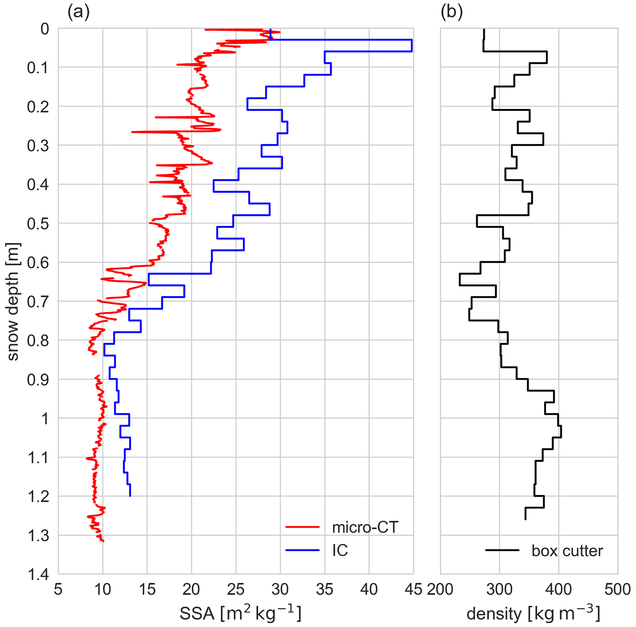
Figure 1The data set with differing SSA measurement results for micro-CT and IC from the Greenland Summit (72∘34′37.9′′ N, 38∘27′03.6′′ W ) expedition in 2015 (Schneebeli et al., 2015). The snow surface is at 0 m. Panel (a) presents the entire SSA profile (about 1.3 m) measured with the micro-CT (red) and IC (blue). The IC has a 3 cm measurement interval. Panel (b) shows the density profile (box cutter, volume 100 cm3).
2.1 Snow sampling and SSA measurements
We use five different alpine snow types with an SSA of between 5 and 25 m2 kg−1 for this study. Type-A snow (Fig. 2a) is a homogeneous alpine settled snow with a decomposed and rounded grain shape, a size between 0.5 and 1.5 mm, and an average density of 235 ± 21 kg m−3 (16 micro-CT samples). Type-B snow (Fig. 2b) is type-A snow that has been stored at −15 ∘C for 13 days in the cold lab under compacting weights. The grain shape is small and rounded, the grain size is medium (0.5 to 1 mm), and the structure is more brittle than that of type A. Type-B snow has an average density of 395 ± 35 kg m−3 (17 micro-CT samples). Type-C snow (Fig. 2c) has large rounded and faceted grains, a size of between 1 and 2.5 mm, and an average density of 322 ± 31 kg m−3 (17 micro-CT samples). Type-D snow (Fig. 2d) has large and rounded grains, a size of between 1 and 2 mm, and an average density of 432 ± 43 kg m−3 (18 micro-CT samples). Type-E snow (Fig. 2e) is refrozen, wet snow with grains that are larger than 2.5 mm and an average density of 302 ± 67 kg m−3.

Figure 2Pictures (Leica Z16 APO) of the undisturbed grain shape and the artificial particles (fragments) for the five snow types that we used for our sampling procedure: (a) rounded and decomposed (type A), (b) small and rounded (type B), (c) large and rounded (facets)(type C), (d) large and rounded (type D), and (e) refrozen, wet snow (type E). The yellow scale bar is 2 mm. We produced the pictures as part of our sampling procedure (see Sect. 2.2).
Additionally, we consider a data set with an artificial snow type (30–80 m2 kg−1) to cover a broad range of SSA values. The artificial snow was produced following Brandt et al. (2011). This snow type is fine-grained snow and consists of spherical particles. It was produced in the cold laboratory at a −20 ∘C room temperature by spraying cold water (Baumann, 2017). The samples were measured using the IC and micro-CT, although not for the optical particle counting.
For our SSA sampling strategy for the IC and micro-CT instruments, we used a homogeneous layer of approximately 6 cm within the snow block of each snow type (A, B, C and D). To identify the homogeneous layer, we performed measurements with a SnowMicroPen (SMP, version 2; Schneebeli and Johnson, 1998). Figure 3 shows the SMP profiles. Due to the highly heterogeneous character of snow type E, we did not obtain an SMP measurement, and we conducted our sampling procedure within the first 6 cm of the snow block. For snow types A, B, C and D, we cut off the unsuitable material above the homogeneous layer. We brushed the surface gently to eliminate loose particles (Fig. 4a) that were produced by the sawing process.
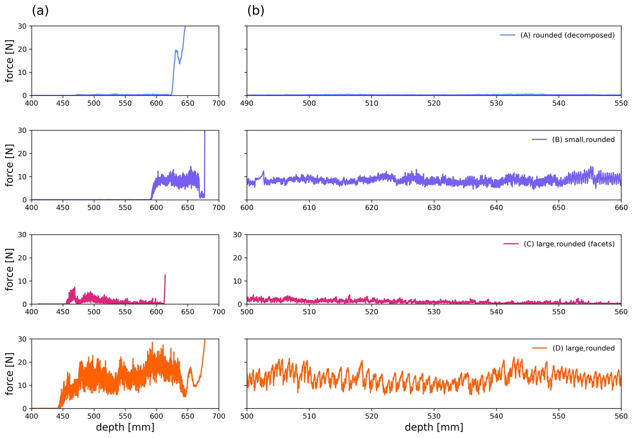
Figure 3SMP measurements (Schneebeli and Johnson, 1998) for snow types A, B, C and D. Snow type E was unsuitable for SMP measurements due to its fragility and heterogeneity. Panel (a) shows the force profile, in newtons, for the whole snow block. Panel (b) displays the homogeneous layer (approximately 6 cm within the snow block) that we used for our sampling procedure.
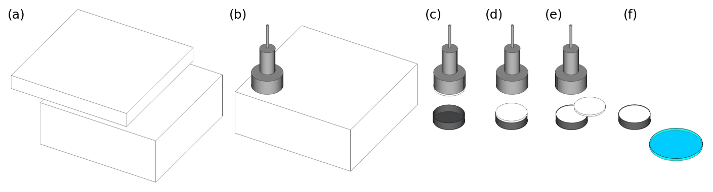
Figure 4Step-by-step illustration of the sampling procedure. (a) Within each snow block (snow types A, B, C and D), we identified a homogeneous layer of snow with SMP measurements. We removed the unsuitable material above the sampling layer with a saw. Afterwards, we gently brushed the surface to remove loose particles from the sawing process. Panel (b) presents the IC sample extraction with the IC sampling device (piston). The snow sample is 35 mm thick. Panel (c) outlines the transfer of the snow sample into the IC sampling holder, which has a height of 30 mm. Panel (d) shows the transferred snow sample with 5 mm of protruding snow. (e) We cut off the protruding snow with a sharp spatula (the sample is slightly tilted), following Gallet et al. (2009), and performed the first IC measurement (IC + particles). (f) We tilted the IC sampling holder above a Petri dish (blue) to collect the remaining loose particles, created during the sampling step shown in panel (e), for further analysis (macro-photographs and particle weight), and the sample was measured again with the IC (IC − particles).
Our sampling procedure starts by retrieving an IC sample (Fig. 4b), following the default method of Gallet et al. (2009) and as described in the IC manual (A2 Photonic Sensors, 2014). We transfer the snow sample from the piston, which is used to retrieve the snow from the snow block or snow cover, respectively, into the 60 mm diameter IC sampling holder (Fig. 4c, d). We then tilt the sample and remove the protruding snow with a spatula (Fig. 4e) to create a flat surface for SSA measurement.
We measure the SSA with the IC in one orientation (IC + particles in Fig. 7) and afterwards again tilt and gently tap the sample over a Petri dish to remove any remaining loose particles from the surface (Fig. 4f). To study the loose particles, we weigh the particle amount in the Petri dish (micro scale ± 0.01 g) and photograph (Leica Z16 APO) the particles (see Sect. 2.2 and Fig. 2). The mass of loose particles is divided by the surface area of the sample holder to retrieve the specific mass (Mspec). Next, we perform a second IC SSA measurement (same sample) without loose particles on the sample surface (IC − particles in Fig. 7). For direct comparison, we take a standard micro-CT sample out of the middle of each IC sample (CT out of IC in Fig. 7). We also retrieve standard micro-CT samples next to the IC samples within the undisturbed snow structure (CT reference in Fig. 7). To provide a meaningful study, we take between five and eight IC samples per snow type and try to preserve this number for each sampling step (Table 1). Due to the fragility of, for example, snow type C, the number of micro-CT samples is not constant.
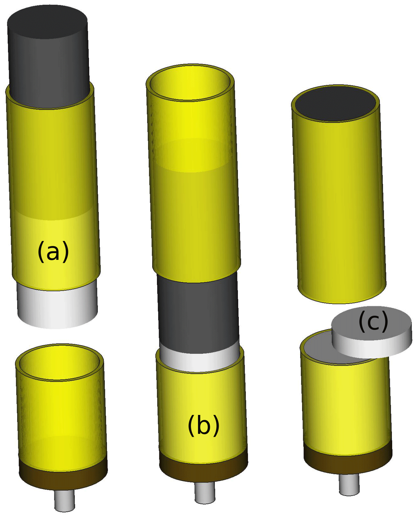
Figure 5Illustration of the micro-CT sampling kit, with the sample holder in yellow, the piston in black and the snow sample in white. Panel (a) presents the manufactured micro-CT sampling kit with the piston imitation (35 mm depth) to retrieve the snow sample. Panel (b) illustrates the snow sample transfer into the sampling holder (30 mm depth), and panel (c) shows the process of cutting protruding snow with a spatula to create a flat sample surface.
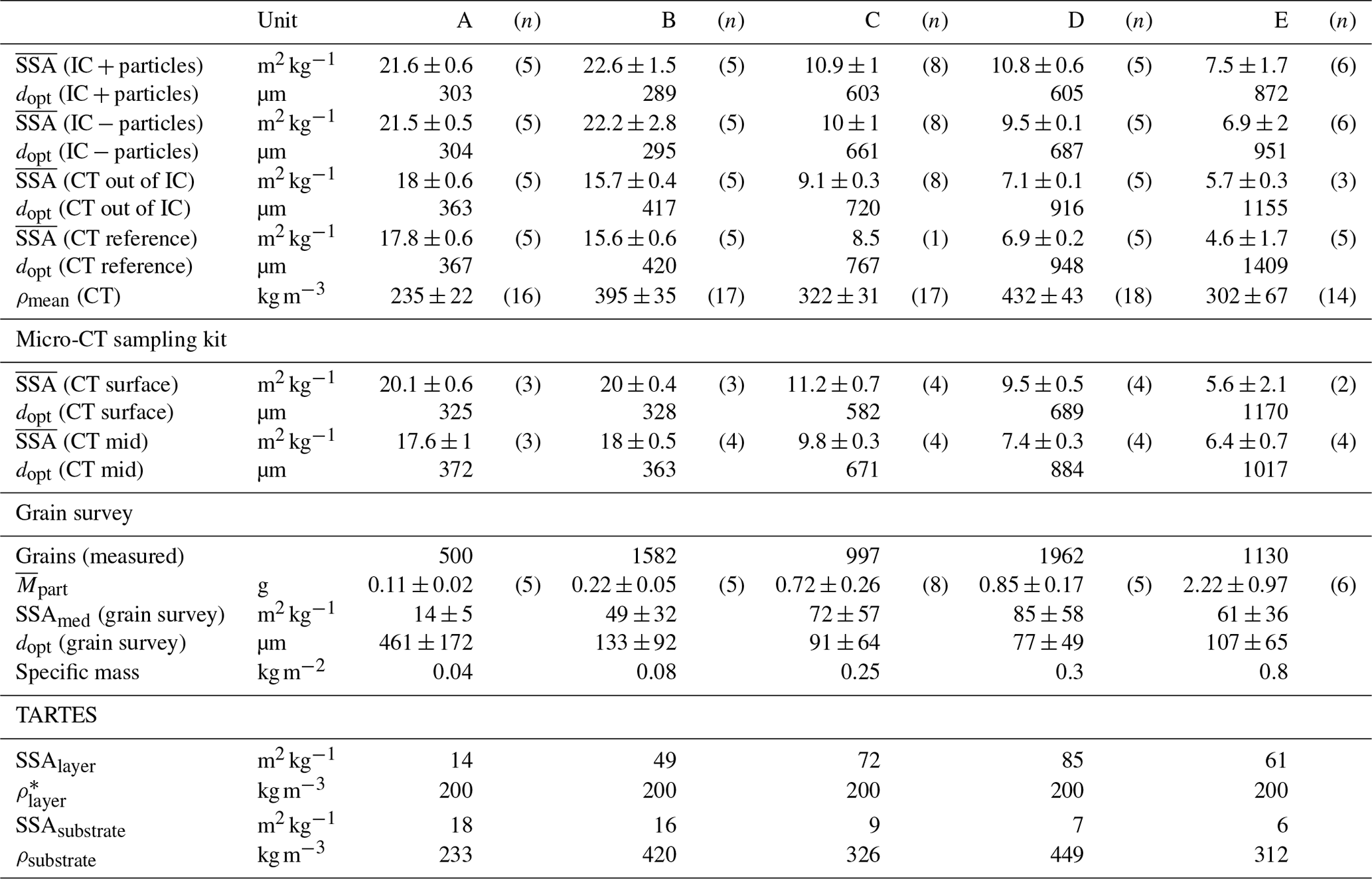
Table 1Means, standard deviations and the number of measurements (n) for all measurements organized following the multi-level sampling strategy. “IC + particles” represents the default sampling procedure suggested by Gallet et al. (2009). The “” row is the synthetic density used for the TARTES simulations. For access to the data set, the reader is referred to the Code and data availability section.
To reproduce the IC's mechanical sampling procedure, we use a specifically manufactured micro-CT sampling kit. The IC has a sampling kit with a 60 mm diameter holder. We manufactured a similar kit for the micro-CT that consists of a piston and a 30 mm diameter sample holder to improve the micro-CT resolution (Fig. 5a); hence, the aforementioned micro-CT kit is an imitation of the IC sampling kit. The same sampling steps are necessary to retrieve the sample from the snow block, including cutting the snow sample surface with a spatula. This allows one to scan, with the micro-CT, for in situ broken particles on the surface produced during the IC-specific sampling procedure (Fig. 5b) and to scan the snow structure deeper in the middle of the sample (Fig. 5c).
We perform all micro-CT measurements with a computer tomography system working in a cold laboratory at −15 ∘C (µCT 40 or µCT 80, Scanco Medical). For comparison with the IC, we measure samples with µCT 40 (55 kVp energy, 15 µm nominal resolution and 145 µA for type A; 55 kVp, 18 µm and 145 µA for types B–E). The µCT 40 has a carousel that allows us to measure up to 10 samples in a row. To measure the micro-CT sampling kit data set, we use the µCT 80 (55 kVp, 15 µm and 145 µA for types A–E). We computed the SSA using the standard segmentation technique described in Hagenmuller et al. (2016).
2.2 Grain survey
We examine and photograph the loose particles created by IC sample preparation in a Petri dish to study their influence on the surface of the IC sample. The Petri dish is subdivided into eight sections and eight circles. By generating random numbers, we receive eight coordinates per sample, resulting in 40 pictures per snow type sample. This procedure guarantees unbiased pictures without a particular preference for the grain shape. To obtain the grain size distribution, we randomly choose eight pictures with about 1000 grains in total for snow types B, D and E. For snow types A and C, we choose 12 pictures to obtain the same number of grains.
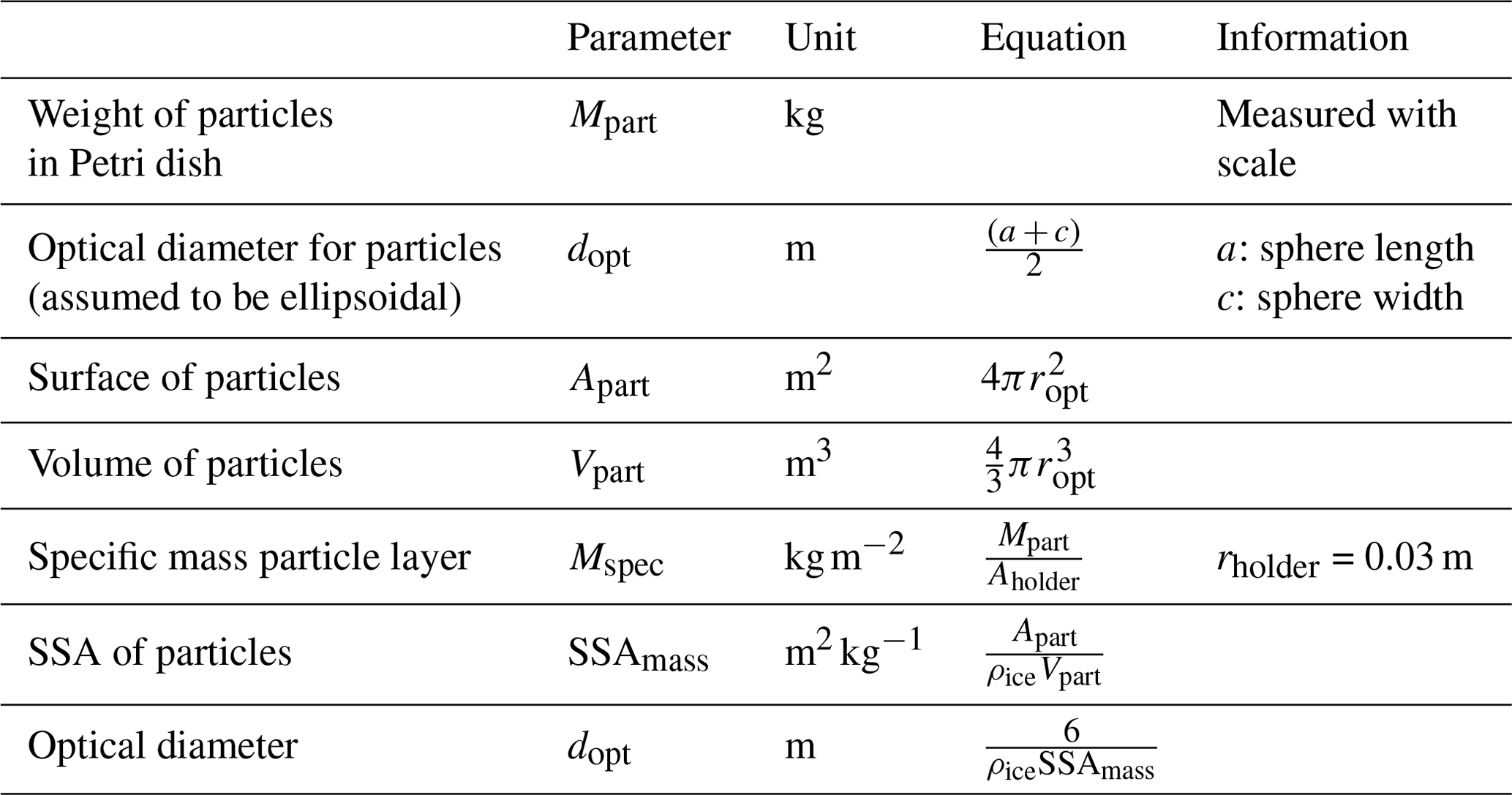
We measure the length and width of every particle with ImageJ (Schneider et al., 2012) and calculate the optical diameter dopt and SSA (SSAmass), assuming the main grain shape to be ellipsoidal. We record the total number of measured grains, the median diameter, the median SSA, the optical diameter dopt and the Mspec for each snow type in Table 1.
2.3 TARTES (Two-streAm Radiative TransfEr in Snow) simulations
To simulate the influence of a layer of artificial particles on top of a substrate snow layer, we use the TARTES model (Libois et al., 2013). The SSA of the particle layer on top is the median SSA that we calculated from the grain examination for each snow type. The density of the particle layers (ρlayer) is set to 200 kg m−3.
We use the average SSA (SSAsubstrate in Table 1) and average density (ρsubstrate in Table 1) of the micro-CT samples out of the IC samples (CT out of IC) as input for the substrate layer below, and the synthetic substrate depth is set to 1 m. In the simulations, we use a 1310 nm wavelength to study the particle influence of the IC operating wavelength and a 950 nm wavelength as an approximation of the near-infrared photography. For the first step, we calculate the diffuse albedo for the two-layer simulation using the albedo function of the TARTES Python module. To calculate the SSA, we needed to apply a conversion to the diffuse albedo data set. Hence, we produced a synthetic SSA data set for both wavelengths, which we use for a poly-fitting procedure. We fit a five-degree polynomial adequate to describe the relationship between the calculated diffuse albedo and the SSA.
Figure 6a shows that the SSA of the artificial snow is the same for both the IC and CT. We measure a lower SSA with the micro-CT for all sintered snow types, independent of the SSA, compared with the IC (Fig. 6b; details in Table 1 and Fig. 7). We also measure a lower SSA with the micro-CT if we scan the prepared flat surface compared with the undisturbed middle of the sample (Fig. 6c) using the micro-CT sampling kit. We now present the detailed results for the different treatments of the samples.
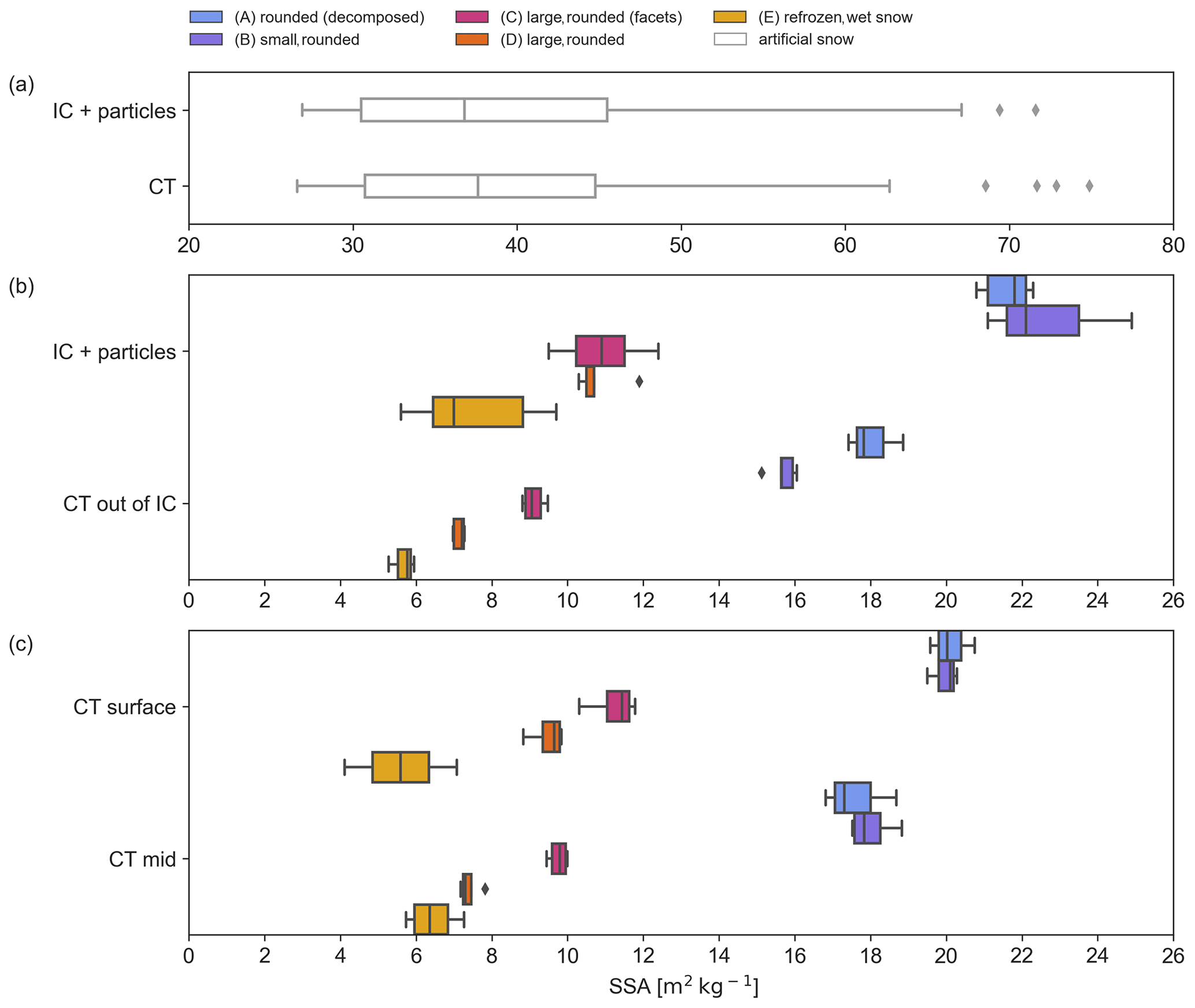
Figure 6All SSA measurements are classified into sampling steps. The box plots represent the median and interquartile range. “IC + particles” is the default method (Gallet et al., 2009; A2 Photonic Sensors, 2014), “CT” represents the micro-CT measurements out of an IC + particles sample, “CT out of IC” denotes the micro-CT measurements out of an “IC − particles” sample, and “CT surface” and “CT mid” refer to the manufactured micro-CT sampling kit. Panel (a) presents the results for the artificial snow data set with SSA values between 30 and 80 m2 kg−1. Panel (b) shows the five snow types (A, B, C, D and E); the SSA is between 5 and 25 m2 kg−1. Panel (c) shows the results for the micro-CT sampling kit with SSA values between 5 and 22 m2 kg−1. All results can be found in Table A1. For access to the data set, the reader is referred to the Code and data availability section.
The artificial snow shows no significant difference between methods (n=45, p=0.43, p < 0.05). The sintered snow types A, B, C and D show a significant difference at the 0.05 level between IC and micro-CT ( (IC + particles) vs. (CT out of IC); see Table 1 and Fig. 7). Type-E snow (four micro-CT samples) had a larger scatter in both IC and micro-CT measurements and is, therefore, not statistically different. However, the SSA is 24 % smaller when measured by the micro-CT compared with the IC.
The removing loose particles (IC − particles) treatment leads to a slight decrease in the IC measurements. The difference between these two sampling steps (IC + particles vs. IC − particles; Tables 1, A1) is not significant for types A, B or E, but it is significant for types C and D. Comparing the IC − particles treatment with micro-CT samples (CT out of IC), the difference is significant for types A, B, C and D (see Table A1). The difference between the micro-CT samples (CT out of IC) and the micro-CT samples taken out of the same snow block next to the IC samples (CT reference) is only significant for snow type D.
Most surface samples measured with the micro-CT sampling kit (Figs. 6c, 8) show a higher SSA than those in the undisturbed middle of each sample. The difference is significant for types C and D. For types A and B, the SSA measured at the sample surface is higher than that measured in the middle of the sample, although not significantly. The SSA at the surface is lower than in the middle for the heterogeneous refrozen, wet snow (type E). Type D shows the highest mean SSA difference (28 %). Figure 8 shows the three-dimensional reconstruction of this particular snow sample. Figure 8a is the sample surface, and Fig. 8b displays the middle. The fragmented artificial particles (less than 0.5 mm) protrude compared with the undisturbed snow structure with a size of 1 mm or more.
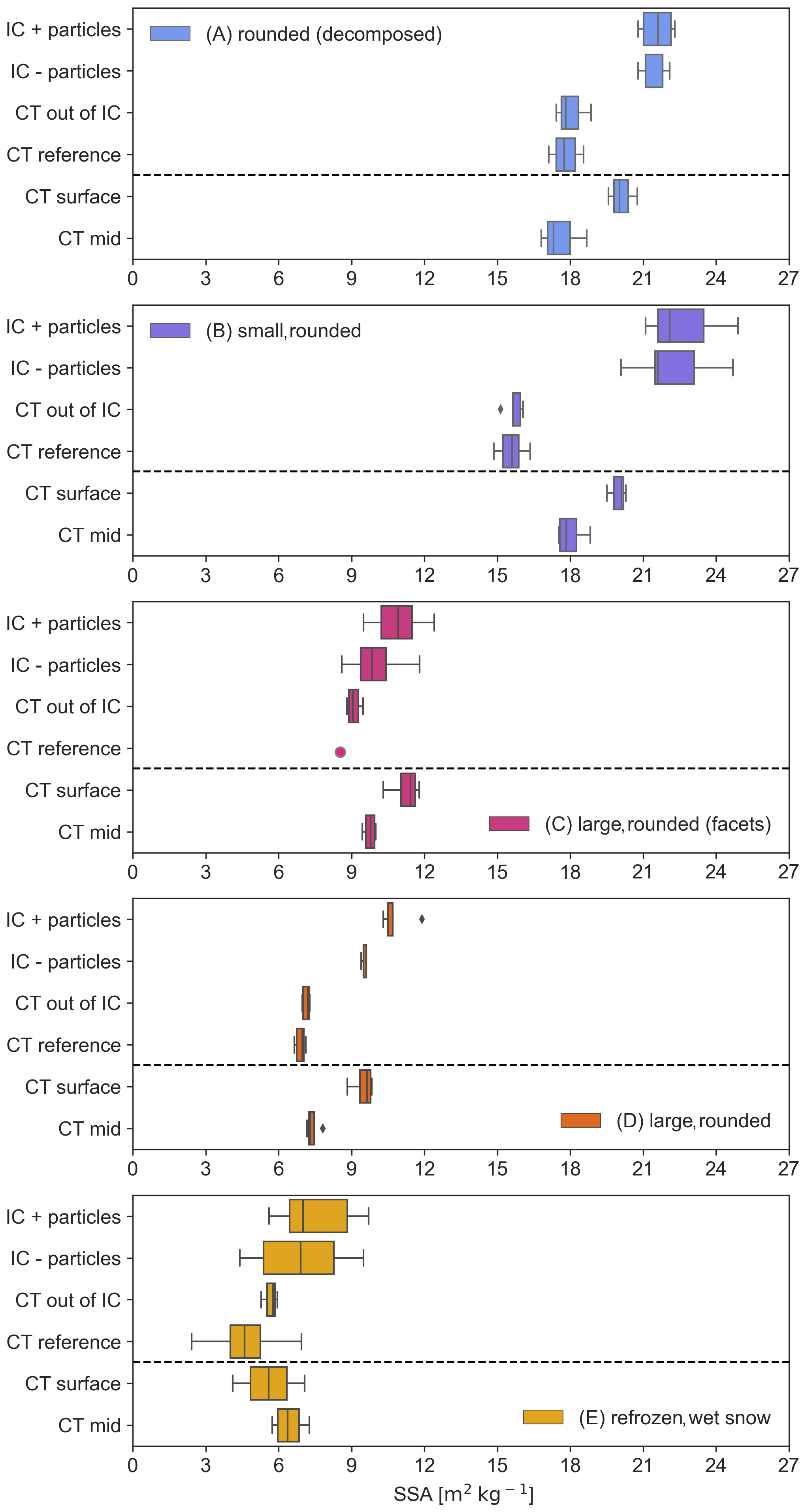
Figure 7All SSA measurements classified into snow types and subdivided into sampling steps; SSA values ranged between 5 and 25 m2 kg−1. “IC + particles” is the default sampling process (Gallet et al., 2009). Results for the micro-CT sampling kit are separated by the dotted grey line in each plot; SSA values ranged between 5 and 22 m2 kg−1. The results can be found in Table 1.
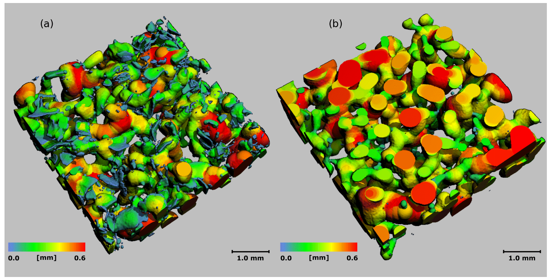
Figure 8A three-dimensional reconstruction for a sample of snow type D taken with the micro-CT sampling kit (Fig. 5). We performed these measurements with the µCT 80 (55 kVp, 15 µm and 145 µA). Panel (a) shows the sample surface scan with artificial particles (< 0.5 mm) prepared following the default IC sampling procedure. Panel (b) shows the snow grains (> 0.5 mm) scanned in the middle of the sample without the influence of the mechanical sampling treatment.
3.1 Grain counting
We examined the size and number of the particles (Table 1) formed at the surface of the micro-CT sampling kit. Table 1 contains the counted number of grains and the weight of particles in the Petri dish. The weight of particles, all measured on the same surface area, varies between 0.11 g and a maximum of 2.22 g, corresponding to a specific mass of 0.04 and 0.8 kg m−2, respectively. The calculated particle median SSA (SSAmed (grain survey); Table 1) is the lowest for type A (14 ± 5 m2 kg−1) and the highest for type D (85 ± 58 m2 kg−1); it is 49 ± 32 m2 kg−1 for type B, 72 ± 57 m2 kg−1 for type C and 61 ± 36 m2 kg−1 for type E. All snow types have a left-skewed particle size distribution. The median optical diameter (dopt (grain survey)) is between 77 ± 49 and 133 ± 92 µm, except for type A (461 ± 172 µm).
We found the following increasing ratio between the optical diameter of the CT reference and the particles: 0.80 – type A, 3.2 – type B, 8.4 – type C, 12.3 – type D and 13.2 – type E. The optical diameter of the particles is smaller than the optical diameter of the undisturbed snow, except for the rounded snow (type A). The ratio and the size show that the sample preparation leads to new small ice particles at the surface. The larger particles of rounded snow (type A) are just at the limit of statistical significance.
3.2 TARTES
Figure 9a displays the influence of the converted SSA with increasing particle layer thickness. Figure 9b shows the percentage change in SSA with increasing particle thickness. Both layers have different SSA and density values (SSAsubstrate and ρsubstrate; Table 1).

Figure 9Simulation of a 1 m thick snow substrate with a thin (< 2.5 mm) particle layer on top with a density of 200 kg m−3. Both layers have different SSA values (Table 1). In panel (a), the TARTES simulations show the SSA at wavelengths of 1310 and 950 nm. Panel (b) presents the percentage change in the SSA for wavelengths of 1310 and 950 nm.
Our TARTES simulations (Fig. 9a) show the SSA at wavelengths of 1310 and 950 nm. Figure 9b shows the percentage change in the SSA for wavelengths of 1310 and 950 nm over increasing particle layer thickness. The SSA for 1310 nm shows a steeper increase with layer thickness compared with that at 950 nm. The SSA of type-A snow shows a slight negative trend with an increase in thickness, as the particle layer SSA is smaller than the substrate SSA. The starting point at 100 % marks the pure substrate SSA for each snow type. The SSA measured at a wavelength of 1310 nm is much more susceptible to the influence of a layer with loose particles. The changes are most prominent for snow types D and E. The slope is about 4 times higher at a wavelength of 1310 nm than at 950 nm.
We found systematic differences between the IC and the micro-CT SSA measurements for snow with an SSA between 5 and 25 m2 kg−1. The most significant difference appears when the sample is prepared following the default sampling procedure. The relative percentage difference ranges from 52 % for type-D snow with a mean bias error (MBE) of 3.7 m2 kg−1 (44 % with a MBE of 7 m2 kg−1 for type B and 32 % with a MBE of 2.2 m2 kg−1 for type E) to 20 % for type A (with a MBE of 3.8 m2 kg−1) and C (with a MBE of 1.8 m2 kg−1). This can be decreased down to 34 % for type D (41 % for type B, 21 % for type E and 19 % for type A) and down to 9 % for type C by removing loose particles. In contrast, we did not find a significant difference in the artificial snow data set with an SSA between 39 and 80 m2 kg−1.
We conclude that the observed difference depends on the predisposition of the snow type to produce small surface particles and is not linked to the SSA. We show that small ice particles form during the flat surface preparation for IC measurements. These particles are preferentially formed from the bonds, as there seems to be a close link to sintering strength. The small particles of the disaggregated snow change the optical properties of the surface and, consequently, lead to an overestimation of the SSA. This partly corresponds to the observations reported by Gallet et al. (2009): they found an overestimation of up to 5 % for hard wind slab layers and suggested brushing the surface to remove particles falsifying the measurement. Gallet et al. (2009) detected an overall accuracy in SSA measurements that was better than 12 % for the DUFISS (DUal-Frequency Integrating Sphere for Snow SSA measurement) device (pre-production model of the IC). Our results indicate that measurements at a wavelength of 1310 nm are prone to systematic biases for most snow types.
The micro-CT sampling kit worked well with respect to reconstructing the IC sampling procedure, and the potential layer of artificial particles on the sample surface became visible (Fig. 8). The discrepancies between the surface and the sample centre, which were between 11 % (type B) and 28 % (type D), support the inference that the number of small particles produced is different for each snow type. The size distributions show most particles to be smaller than 133 µm for types B, C, D and E, which does not correspond to the grain size of the original snow. For each snow type except type A, the survey reveals an optical diameter of at least half the size (type B: 133 µm) compared with the optical diameter estimated from the SSA measured with the IC (type B: 289 µm) and at least 3 time times smaller than the optical diameter from the CT measurements (type B: 417 µm). For snow types C, D and E, the dopt is between 54 % (type B) and 88 % (type E) smaller compared with measurements with the IC and between 68 % (type B) and 91 % smaller compared with the CT out of IC measurements. The rounded grain of type-A snow appears to be very fragile and does not produce small particles. Consequently, the broken particles are very similar in size to the undisturbed snow.
The TARTES simulations show that the albedo at a wavelength of 950 µm is more robust and less susceptible to an artificial particle layer compared with the albedo at 1310 µm. The simulations at a wavelength of 1310 µm explain the deviation in SSA between the IC and the micro-CT reasonably. For the more fragile snow types (C, D and E), a particle layer thickness of less than 0.5 mm bridges the deviation. A 1 mm thick particle layer can explain the deviation for the less sensitive type-B snow. Type-A snow shows no effect of a particle layer. The reason for this is that the e-folding depth at 950 nm is about twice that at 1310 nm. Gallet et al. (2009) chose 1310 nm, as the absolute reflectance difference for the relevant SSA is larger at this wavelength than at 950 nm. However, the precision of the measurement depends not only on the absolute reflectance difference but also on the signal-to-noise ratio of the receiver, either a photodiode (in the case of a point instrument) or a charge-coupled device (in the case of a camera).
We finally conclude that the measured differences in SSA of the strongly sintered snow from the Greenland Summit expedition (Fig. 1) are explained by the formation of small particles during IC sample preparation.
The key to explaining the deviation between IC and micro-CT SSA measurements is the mechanical destruction of parts of the original snow structure into small, artificial particles during the sample preparation process. Those particles lead to an SSA overestimation by the IC. The formation of these particles is related to different variables, such as SSA, temperature, grain shape and sampling treatment. Fresh, poorly bonded snow with a high SSA shows a negligible effect; the same is found for rounded snow, although to a lesser degree. The measured difference between micro-CT and IC is, however, not limited to a specific geographic origin of the snow. We can simulate the SSA bias effect using TARTES simulations. The formation of small particles at the surface is a systematic source of bias in spectroscopic measurements. We found that the IC overestimated the SSA and underestimated the optical diameter for most snow types in our study. Additional sample surface preparation steps, such as brushing or vacuuming, could be applied, but the outcome and benefits are uncertain and need further investigation.
Table A1Summary of the statistical analyses. The first step was to test for a normal distribution. Testing for significant differences between the sampling steps was then carried out. “IC + particles” represents the default sampling procedure suggested by Gallet et al. (2009).
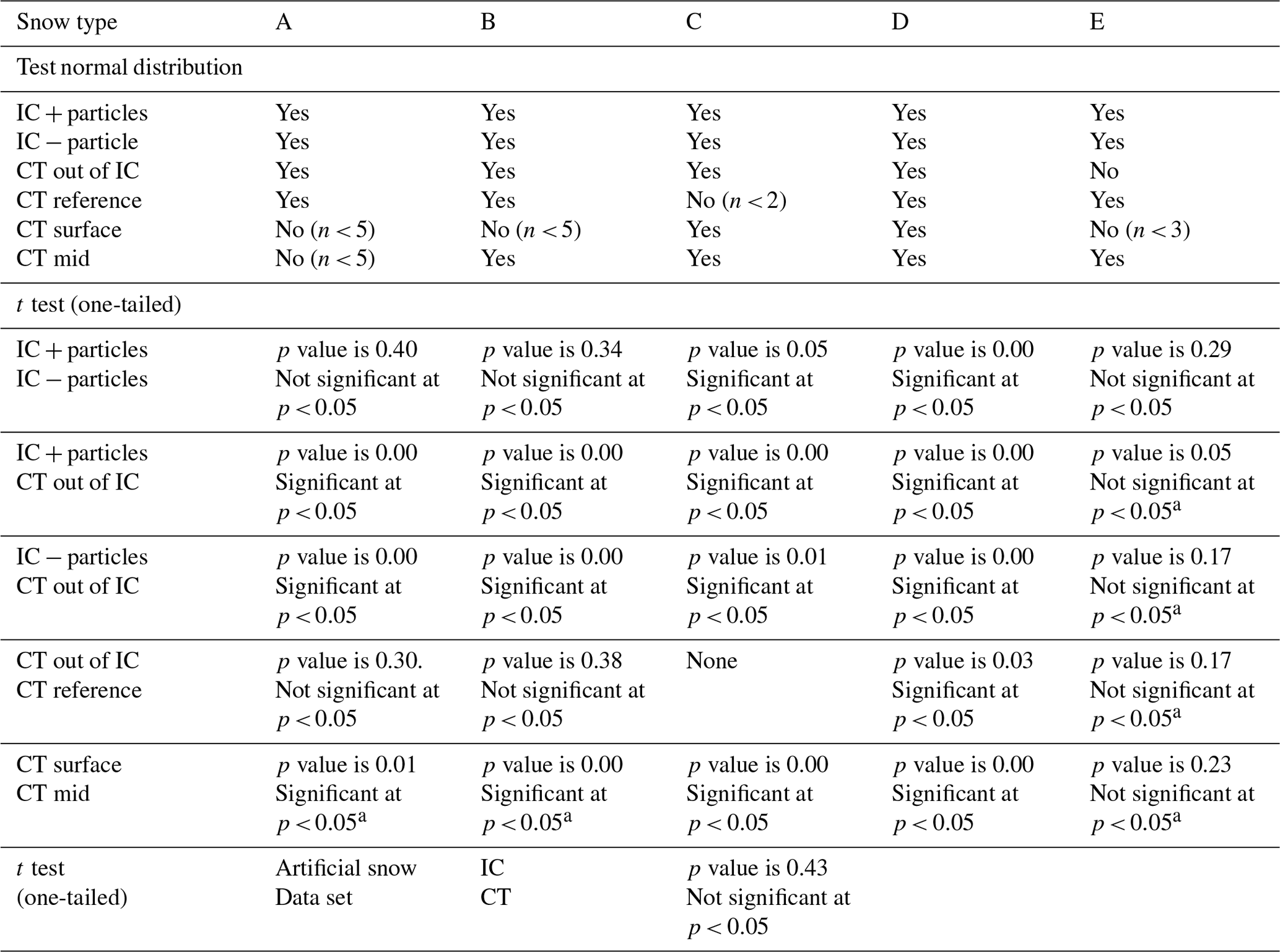
a Data sets for which at least one of the two sample groups is not normally distributed but is assumed for t-testing.
Table A2The equations used in this paper, including parameters and units.
The data set and the source code for the TARTES simulation are available from https://doi.org/10.16904/envidat.333 (Martin and Schneebeli, 2022).
JM and MS designed the study and conceptualized the data collection. JM carried out the measurements and the simulations. JM and MS interpreted the results. JM wrote the first draft of the paper, and MS contributed to the paper.
The contact author has declared that none of the authors has any competing interests.
Publisher’s note: Copernicus Publications remains neutral with regard to jurisdictional claims in published maps and institutional affiliations.
The authors are sincerely grateful to Henning Löwe for his ongoing support, enthusiasm and valuable comments. We would also like to thank Martin Proksch, Margret Matzl and Lino Schmid for the Greenland Summit 2015 data set contribution. Furthermore, we appreciate the work of Philipp Baumann, who provided the artificial snow data set.
The article processing charges for this open-access publication were covered by the Alfred Wegener Institute (AWI), Helmholtz Centre for Polar and Marine Research.
This paper was edited by Melody Sandells and reviewed by two anonymous referees.
A2 Photonic Sensors: User Manual: IceCube Optical system for the measurement of the specific surface area (SSA) of snow, Tech. rep., 2014. a, b
Baumann, P.: Influence of black carbon on the measurement of the specific surface of snow with the near infrared method, Tech. rep., https://doi.org/10.16904/envidat.333, 2017. a
Brandt, R. E., Warren, S. G., and Clarke, A. D.: A controlled snowmaking experiment testing the relation between black carbon content and reduction of snow albedo, J. Geophys. Res.-Atmos., 116, D08109, https://doi.org/10.1029/2010JD015330, 2011. a
Domine, F., Taillandier, A. S., and Simpson, W. R.: A parameterization of the specific surface area of seasonal snow for field use and for models of snowpack evolution, J. Geophys. Res., 112, 1–13, https://doi.org/10.1029/2006JF000512, 2007. a
Domine, F., Albert, M., Huthwelker, T., Jacobi, H.-W., Kokhanovsky, A. A., Lehning, M., Picard, G., and Simpson, W. R.: Snow physics as relevant to snow photochemistry, Atmos. Chem. Phys., 8, 171–208, https://doi.org/10.5194/acp-8-171-2008, 2008. a
Gallet, J.-C., Domine, F., Zender, C. S., and Picard, G.: Measurement of the specific surface area of snow using infrared reflectance in an integrating sphere at 1310 and 1550 nm, The Cryosphere, 3, 167–182, https://doi.org/10.5194/tc-3-167-2009, 2009. a, b, c, d, e, f, g, h, i
Gallet, J.-C., Domine, F., and Dumont, M.: Measuring the specific surface area of wet snow using 1310 nm reflectance, The Cryosphere, 8, 1139–1148, https://doi.org/10.5194/tc-8-1139-2014, 2014. a
Hagenmuller, P., Matzl, M., Chambon, G., and Schneebeli, M.: Sensitivity of snow density and specific surface area measured by microtomography to different image processing algorithms, The Cryosphere, 10, 1039–1054, https://doi.org/10.5194/tc-10-1039-2016, 2016. a
Kerbrat, M., Pinzer, B., Huthwelker, T., Gäggeler, H. W., Ammann, M., and Schneebeli, M.: Measuring the specific surface area of snow with X-ray tomography and gas adsorption: comparison and implications for surface smoothness, Atmos. Chem. Phys., 8, 1261–1275, https://doi.org/10.5194/acp-8-1261-2008, 2008. a
Libois, Q., Picard, G., France, J. L., Arnaud, L., Dumont, M., Carmagnola, C. M., and King, M. D.: Influence of grain shape on light penetration in snow, The Cryosphere, 7, 1803–1818, https://doi.org/10.5194/tc-7-1803-2013, 2013. a
Martin, J. and Schneebeli, M.: IceCube_microCT_Snow_grainsize, EnviDat [code, data set], https://doi.org/10.16904/envidat.333, 2022. a
Morin, S., Domine, F., Dufour, A., Lejeune, Y., Lesaffre, B., Willemet, J. M., Carmagnola, C. M., and Jacobi, H. W.: Measurements and modeling of the vertical profile of specific surface area of an alpine snowpack, Adv. Water Resour., 55, 111–120, https://doi.org/10.1016/j.advwatres.2012.01.010, 2013. a
Schneebeli, M. and Johnson, J. B.: A constant-speed penetrometer for high-resolution snow stratigraphy, Ann. Glaciol., 26, 107–111, https://doi.org/10.3189/1998AoG26-1-107-111, 1998. a, b
Schneebeli, M., Proksch, M., Matzl, M., and Schmid, L.: 2015 Greenland data set (unpublished), EnviDat [code, data set], https://doi.org/10.16904/envidat.333, 2015. a, b
Schneider, C. A., Rasband, W. S., and Eliceiri, K. W.: NIH Image to ImageJ: 25 years of image analysis, 9, 671–675, https://doi.org/10.1038/nmeth.2089, 2012. a