the Creative Commons Attribution 4.0 License.
the Creative Commons Attribution 4.0 License.
 | 13 Apr 2023
First observations of sea ice flexural–gravity waves with ground-based radar interferometry in Utqiaġvik, Alaska
Dyre Oliver Dammann
Mark A. Johnson
Andrew R. Mahoney
Emily R. Fedders
We investigate the application of ground-based radar interferometry for measuring flexural–gravity waves in sea ice. We deployed a GAMMA Portable Radar Interferometer (GPRI) on top of a grounded iceberg surrounded by landfast sea ice near Utqiaġvik, Alaska. The GPRI collected 238 acquisitions in stare mode during a period of moderate lateral ice motion during 23–24 April 2021. Individual 30 s interferograms exhibit ∼ 20–50 s periodic motion indicative of propagating infragravity waves with ∼ 1 mm amplitudes. Results include examples of onshore wave propagation at the speed predicted by the water depth and a possible edge wave along an ice discontinuity. Findings are supported through comparison with on-ice Ice Wave Rider (IWR) accelerometers and modeled wave propagation. These results suggest that the GPRI can be a valuable tool to track wave propagation through sea ice and possibly detect changes in such properties across variable ice conditions.
- Article
(9683 KB) - Full-text XML
-
Supplement
(33081 KB) - BibTeX
- EndNote


Ocean waves play an important role, impacting the formation, dynamics, and breakup of sea ice as established by numerous studies (Squire et al., 1995; Squire, 2007). Waves in sea ice have gained increasing attention in recent years due to rapid loss of sea ice in the Arctic (Yadav et al., 2020) leading to enhanced fetch. This is expected to increase ocean wave activity and the generation of swells which can penetrate far into the ice pack as flexural–gravity waves (Kohout et al., 2015). The propagation of infragravity waves through sea ice is complex, as it depends upon resonant frequencies and can lead to leaky waves and edge waves along boundaries (Kovalev et al., 2020; Kovalev and Squire, 2020). Propagation of waves can in turn induce fracture and break up ice floes into smaller pieces, further accelerating sea ice decline (Thomson and Rogers, 2014).
The recognized significance of waves in ice and their dispersion and attenuation led to several advances in in situ and remote sensing methods as well as multiple scientific experiments conducted from drifting sea ice (Squire, 2018). Early assessments of wave propagation in sea ice were carried out using wire strain gauges (Squire, 1978) and used to detect “ice-coupled” flexural–gravity waves in landfast sea ice (Crocker and Wadhams, 1988). Tiltmeters were later utilized with easier deployment and maintenance (Czipott and Podney, 1989) partially through self-leveling mechanisms (Doble et al., 2006). Several other techniques have also proven valuable for wave detection in sea ice, such as buoys, upward-looking sonar (Thomson et al., 2019), and ship-based stereo imagery (Smith and Thomson, 2020).
Accelerometers are commonly utilized to measure waves in sea ice (Kohout et al., 2015; Sutherland and Rabault, 2016) and have significantly improved over the years (Doble et al., 2006) partly due to open-source components (Rabault et al., 2020). In this work, we utilize a system named Ice Wave Rider (IWR) which is based on the VN-100 inertial measurement unit (IMU) manufactured by VectorNav. This system measures three-dimensional acceleration at 10 Hz with a three-axis accelerometer and a three-axis gyroscope. The components are enclosed in a Pelican Storm Case and can be strapped down to the ice for 60 d deployments with Iridium telemetry of data (Johnson et al., 2020).
Remote sensing approaches have also been used to evaluate waves including optical and radar altimetry (Collard et al., 2022) as well as lidar altimetry to evaluate waves in the marginal ice zone (Horvat et al., 2020). Synthetic-aperture radar (SAR) has been used to estimate wave orbital velocity and wave height from backscatter distortion (Ardhuin et al., 2015, 2017) and map wave fields through interferometry (Mahoney et al., 2016). These satellite-based approaches are valuable for evaluating waves in sea ice over large spatial scales but are limited in temporal sampling. A higher sampling can be obtained with airborne systems (Sutherland et al., 2018), but logistics and cost can limit sampling to hours. For longer-term observations of sea ice motion and deformation, a ground-based system can be a more practicable solution.
In a recent study, Dammann et al. (2021a) used a GAMMA Portable Radar Interferometer (GPRI) stationed on floating sea ice to observe microscale horizontal strain. This demonstrated the ability of the GPRI to quantify and separate transient processes from a large-scale strain field and dynamically discriminate between regions of different properties. Additional work has been done to observe landfast sea ice from shore using a GPRI to discriminate stabilized zones and monitor ice movement in response to wind and current conditions (Dammann et al., 2023). A key motivation for such work has been to investigate the potential for the GPRI system for seasonal monitoring of landfast ice and evolving stability due to changing ice and environmental conditions. This could help determine the applicability of the GPRI to detect conditions or dynamics as precursors to ice failure and breakout events such as horizontal strain and tidal displacement (Dammann et al., 2023). However, an open question has been whether the GPRI could characterize waves in sea ice which together with long-term strain monitoring could help characterize ice conditions and impacts of waves on ice stability.
With only a limited GPRI dataset obtained from a grounded iceberg near Utqiaġvik, Alaska, in April 2021, we demonstrate in this paper the application for monitoring millimeter-scale waves in landfast sea ice. First, we model the expected results from idealized harmonic waves and compare these with GPRI observations. Second, we compare observations with ice displacement data derived from three IWRs deployed on the ice. Finally, we discuss wave properties, accuracy, and limitations due to secondary vertical and horizontal motion.
2.1 Ground-based radar interferometry of sea ice
In this work, we utilize the GAMMA Portable Radar Interferometer (GPRI). This coherent radar system is capable of detecting millimeter-scale displacements in sea ice through interferometry, i.e., the assessment of the phase change, ΔΦ, in the radar backscatter over time (Dammann et al., 2021a). ΔΦ is proportional to the component of surface displacement resulting in a slant range, allowing for relative horizontal displacement, dhr, or relative vertical displacement, dvr, to be calculated from the observed ΔΦ as follows:
which depend on the signal wavelength, λs=0.017 m, and incidence angle, θ. For a GPRI system elevated above the ice surface, both horizontal and vertical motion can result in a significant change in slant range in the near field, within a few hundred meters of the GPRI. In this range, geometric constraints are required to resolve ambiguity between vertical and horizontal motions. Beyond such a distance, instrument sensitivity to vertical motion becomes negligible as the incidence angle, θ, approaches 90∘, and all phase changes can be interpreted as horizontal.
The accuracy of the phase-derived ice motion depends on the interferometric coherence, a measure of how stable the reflected radar signal is over time, ranging between 0 (incoherent) and 1 (completely coherent). For points on the ice with high coherence, e.g., >0.9, accuracy can reach the sub-millimeter scale (Dammann et al., 2021a). However, accuracy can also be impacted by antenna movement (e.g., due to unstable GPRI footing) (Dammann et al., 2021a) or changing atmospheric conditions (Dammann et al., 2023). The GPRI can be operated in either of two modes, scan mode, in which the antennas rotate while acquiring data, or stare mode, where an image is acquired while looking in a fixed orientation. Here, we apply the stare mode, in which the GPRI collects continuous measurements in one direction at 100 Hz. The observations are interpreted as coming from a narrow (one-dimensional) strip, as the antenna generates a fixed fan beam spreading 0.4∘ in azimuth. Individual observation time spans were limited to 30 s. During these sub-minute windows, we expect atmospheric contributions to be negligible.
In stare mode, interferograms are oriented in range-time space, where each row represents the phase change since the start of the acquisitions. Each row thus represents cumulative phase change up until a particular time, and each column represents a particular range point on the ice in the line-of-sight (LOS) direction from the GPRI. We process all the interferograms by first temporally averaging them to effectively reduce speckle and decrease the temporal sampling to 20 Hz. Then, we interpret the progressive ΔΦ over 30 s as vertical displacement according to Eq. (1) and subtract the mean displacement to easier identify the wave motion. We then subset the 30 s displacement time series based on low variability (RMSE <0.3–0.5 mm compared to a 1 s running mean). The reduced sensitivity to vertical motion with range in combination with small, ∼ 1 mm observed waves was found to be optimal for limiting observations within 200 m of the GPRI and in areas with high coherence (>0.999) to ensure low noise in the observations.
2.2 Observations at Utqiaġvik
We carried out a series of 30 s long observations on the landfast sea ice near Utqiaġvik during April–May 2021. The landfast ice consisted of first-year sea ice and incorporated a large iceberg grounded at 10 m depth ∼ 2 km offshore. We stationed a GPRI on top of the iceberg ∼ 6 m above sea level (Fig. 1a). The radar alternated between staring in a direction across and along a ∼ 200 m wide refrozen lead (cyan lines in Fig. 1b) with a 2 min lag repeated every 10 min, totaling 238 acquisitions. Within 200 m from the GPRI, we expect the vertical sensitivity to be sufficient to pick up vertical motion. Clear wave signals were only identified with the GPRI facing across the lead (solid cyan line) possibly due to the smooth, uniform ice conditions. We also deployed three Ice Wave Riders (IWRs) on the ice in the vicinity of the GPRI (green triangles in Fig. 1a). These deployments enable a comparison between IWR- and GPRI-derived ice surface motion during only two across-lead acquisitions in which data overlapped (Table 1).
We evaluate ice thickness using measurements obtained between 16 April and 5 May 2021 as part of an annual community ice-trail-mapping project in Utqiaġvik. Ice thickness is derived from electromagnetic conductivity measurements obtained with a snow machine pulling a GPS-equipped Geonics EM31-MK2 ground conductivity meter (Druckenmiller et al., 2013). Measurements were collected every second at speeds <5 m s−1, ensuring ice thickness measurements no more than 5 m apart. Ice thickness ranged from 0.6 m to several meters thick with areas of smooth ice being ∼ 1 m thick.
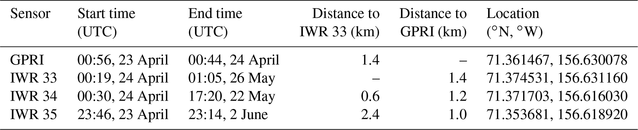
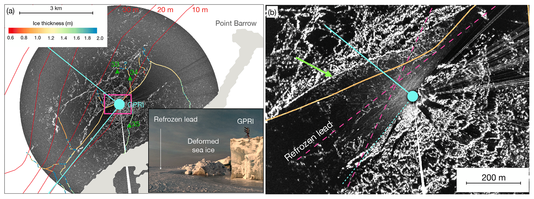
Figure 1(a) Location of the GPRI superimposed on scan-mode backscatter imagery. The GPRI stared in the direction of the cyan lines. Bathymetry contours are drawn in red. Location of IWRs is identified with green triangles. Multi-colored line shows ice thickness as indicated by the color bar. Land is masked out in light gray. The pink rectangle indicates the location of the zoomed-in area in panel (b). (b) Zoomed-in area of the refrozen lead adjacent to the GPRI. The dashed pink lines indicate possible directions of wave propagation commented on in the text. The green arrow in panel (b) indicates the deformed offshore edge of the refrozen lead.
2.3 Modeling wave dispersion and expected impact on stare-mode interferometry
We model vertical ice displacement, dv, in response to harmonic waves to investigate how the GPRI can be used to detect and characterize waves in sea ice:
where A is the amplitude, x is the distance from the GPRI, k is the wavenumber , where λw is the wavelength of the propagating wave), ω is the angular frequency (, where T is the wave period), t is the time, and φ0 is the phase of the surface wave at t=0. If the GPRI is placed on a fixed location, e.g., the shore or firmly grounded ice, the vertical ice surface displacement relative to the GPRI, , will be equal and opposite of the actual surface motion, that is
We can model interferograms by substituting for dvr in Eq. (2). To best illustrate this, we model waves with a period half of the observation window (T=15 s) in water depth, e.g., H=10 m (based on bathymetric contours in Fig. 1). According to the shallow-water approximation, the wave speed can be approximated to c≈9.9 m s−1 through the following expression based on gravity, g, and water depth, H:
We obtained the same speed, c, using the full dispersion equation (Johnson et al., 2021) and ∼ 1 m ice thickness based on the EM31 survey. Through c, we can also approximate λw=150 m for T=15 s. The resulting and associated interferogram is displayed in Fig. 2a and b respectively. ΔΦ is most significant in the near range due to the decreasing sensitivity of the GPRI to vertical motion with increasing range. ΔΦ exhibits a periodic, diagonal pattern where we can identify both the wave period and observed speed, co, based on the pattern spacing and angle respectively (Fig. 2b).
The speed observed with the GPRI, co, will differ from the speed of the wave, c, and depends upon the angle, α, between the GPRI LOS and the propagation direction of the wave; i.e., if α is non-zero, c0 will be greater than c because LOS distance between crests will be greater than the wavelength, λw:
Incoming shallow-water waves typically propagate perpendicular to bathymetric contour lines as the wave speed decreases with decreasing depth (Eq. 5). The LOS direction of the GPRI intersected the local isobaths approximately 15∘ from normal (Fig. 1a); hence we expect to observe ∼ 10 m s−1 for waves propagating from the offshore region (modeled in Fig. 2b). Inhomogeneities in the ice cover such as changing ice thickness, fractures, and rough ice can result in altered directionality of wave propagation. As an example, is expected to result in co=38 m s−1 and the observed interferogram in Fig. 2d. If the GPRI is placed on floating ice (subject to vertical and horizontal motion due to sensor uplift and tilt), the phase patterns will be more challenging to interpret. This is further discussed in Appendix A.
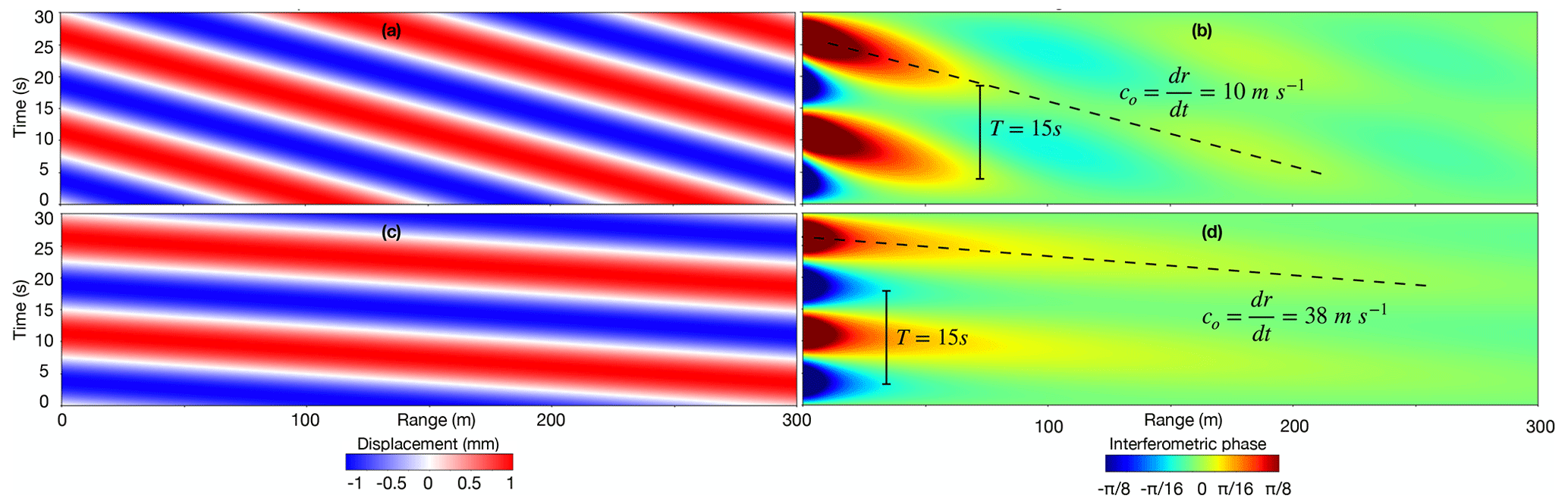
Figure 2(a) Relative vertical elevation (i.e., elevation difference between the GPRI and the ice surface) for simulated periodic oscillations in 10 m water depth (T=15 s, A=1 mm, λw = 150 m) for LOS parallel to wave propagation and (b) associated synthetic interferogram. Panels (c) and (d) show results for the same simulated oscillations but with a LOS at 75∘ to the direction of propagation. The phase magnitudes of the patterns in panels (b) and (d) will differ based on the elevation of the GPRI system above the ice surface (here 6 m).
2.4 Modeling superposition of infragravity waves and impact on stare-mode interferometry
During the season and in the region considered here around Utqiaġvik, Alaska, sea ice is widespread. From the dispersion relation the effects of sea ice on waves arise as products of the bending modulus and compressive stress terms times higher powers of the wavenumber (see Johnson et al., 2021, and references therein). These terms become small for the relatively long infragravity waves, meaning ice has little effect. Sea swell on the other hand is significantly damped by the presence of sea ice (Bromirski et al., 2010). We have shown previously that infragravity waves can propagate over long distances across the ice-covered Arctic Ocean (Mahoney et al., 2016). As ocean swell is damped in an ice-covered sea, we assume that the wave forcing in this region is dominated by infragravity waves generated in the open ocean potentially hundreds of kilometers away (Bromirski et al., 2010, 2015). These waves are dispersive (Bromirski et al., 2010, 2015) so that the signals arriving in the vicinity of the GPRI are close to monochromatic during the short window of observations.
The modeled example (Eq. 3 and Fig. 2) demonstrates a single wave field. However, even with monochromatic infragravity waves, two wave fields can occur in sea ice when waves reflect off and propagate along inhomogeneities such as cracks and ridges (e.g., edge waves) (Marchenko and Semenov, 1994; Marchenko, 1999) and interact with the general wave field. Such a reflected wave will have a similar period and speed, c, as the incoming wave field but with different observed speed, co. Hence, the resulting observed wave speed from individual observed waves co1 and co2 is (. In the case of a secondary wave field interfering, the superimposed waves can be expressed as
where and represent average values of the two waves. The phase speed of the combined wave field, represented by the first term in Eq. (7), is the average speed of the two waves. To illustrate this, we model a single infragravity wave field (Fig. 3a) and superimpose an edge wave with co2=2co1 (Fig. 3b). We also model a standing wave as a result of a wave reflecting off a wall in the case that the amplitude is conserved (Fig. 3c). This is a potential scenario for waves interacting with the lead boundary/iceberg but with uncertainties related to reflected amplitude and propagation angles.
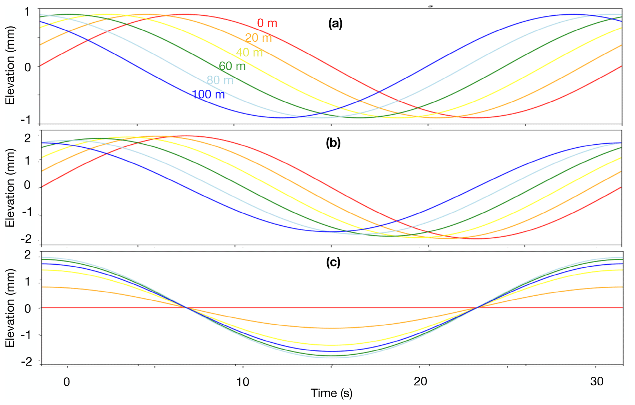
Figure 3Modeled vertical displacement in the GPRI LOS direction at different positions in range in the following cases. (a) A single wave field with co=10 m s−1, λ=300 m, A=1 mm, and T=30 s. (b) The wave field in panel (a) superimposed on a wave field with the same A and T as in panel (a) but where co=20 m s−1 and λo=600 m. (c) A standing wave expected from an ideal reflection of the wave in panel (a). Colors represent different locations in range from 0 (red) to 100 m (blue).
2.5 Deriving wave properties from Ice Wave Rider data
We interpret the vertical acceleration from the IWRs in the form of the power spectral density. This is derived by partitioning the acceleration time series into 15 min segments with a 50 % overlap and smoothing twice in frequency with a 1–2–1 weighting. We then display the amplitude–frequency distribution over time in the form of Welch periodograms. This enables the identification of ubiquitous bursts of activity typically less than 15 min (see example in Fig. 4). We can estimate the predominate direction of wave propagation from the cross-correlation lag time, l, in between the acceleration signals measured at IWR 33 and IWR 34:
where d=630 m is the distance in between the IWRs and ψ is the propagation angle relative to the direct line in between the IWRs. We assume a similar wave speed as before of c=9.9 m s−1, as the ice in between the sensors was mostly smooth and estimated at ∼ 1 m thickness based on the nearby EM31 survey. A maximum correlation lag is thus expected to be l=64 s (ψ=0) and l=63 s for waves propagating directly onshore (). We derive the amplitude from the partitioned acceleration, az, as described by Kohout et al. (2015) and further detailed in Rabault et al. (2020):
We use a low-frequency cutoff of T=60 s, double the acquisition window of the GPRI. Lower-frequency waves will thus be difficult to detect within the 30 s GPRI window and will start to resemble uniform sea level change.
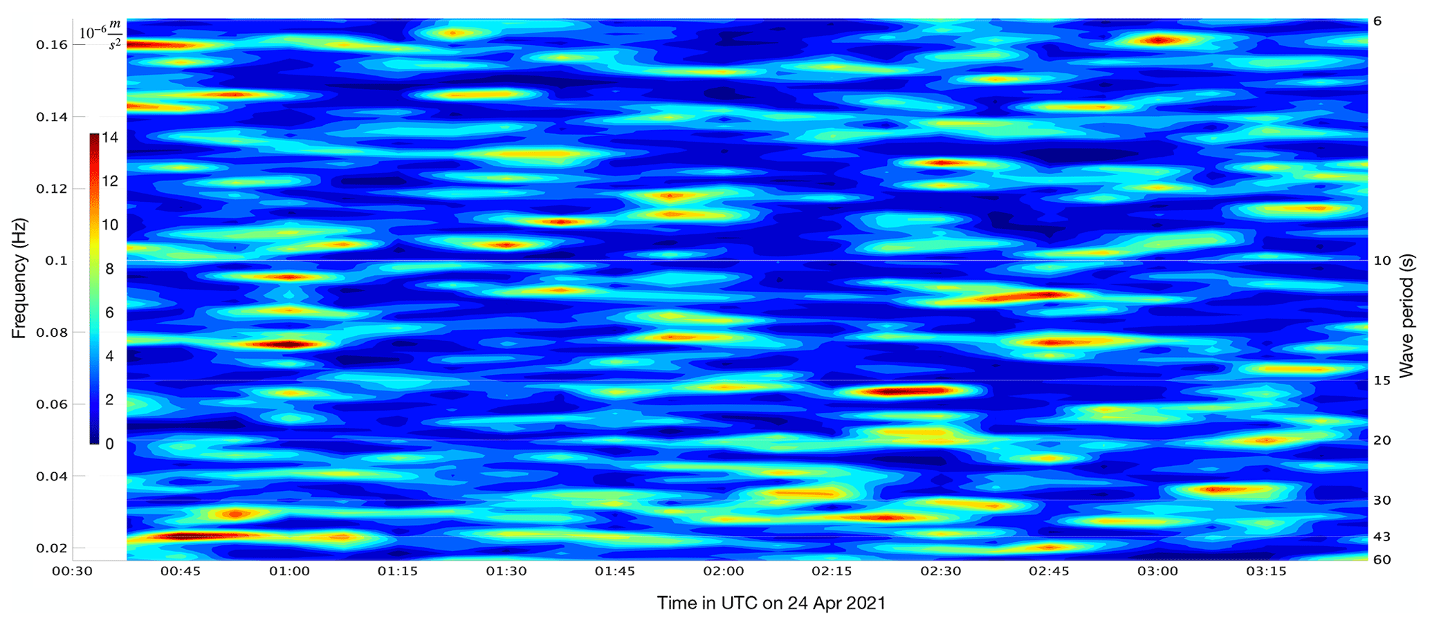
Figure 4Example of vertical acceleration measured by IWR 33 during the first ∼ 3 h after deployment on 24 April 2021. The acceleration is displayed as the power spectral density in the frequency–time domain as in a Welch periodogram. Numbers ranging from 6 to 60 to the right of the figure are period values in seconds corresponding with the frequency axis on the left-hand side.
3.1 Comparison of observations with a modeled wave
A good example of a surface-wave-like signal detected by the GPRI is the interferogram acquired on 23 April at 21:56 UTC (referred to as E1), where a negative ΔΦ signal (i.e., positive vertical displacement according to Eq. 2) appears after the first ∼ 15 s and propagates towards the GPRI over the last ∼ 15 s (Fig. 5a). To demonstrate the similarity with a wave signal, we model a wave according to Eq. (3) from a fixed GPRI position. We model the wave with approximate wave properties based on the observations (λw=0.3 km, A=0.9 mm, and T=30 s). The similarity of interferometric-phase patterns between the observations and model (Fig. 5a and b respectively) confirm that the GPRI did not tilt significantly during acquisition and can therefore be treated as a fixed deployment. Although the single observed wave observed in Fig. 5a matches closely with the modeled wave field, it is worth noting that it lacks the sign of the prior wave modeled as a second positive signal (red area in the bottom of Fig. 5b). This suggests that although we observe an onshore wave, it may not be a part of a strict monochromatic wave field. Also, some vertical lines in Fig. 5a differ significantly from surrounding lines and Fig. 5b, as they represent locations with low coherence.
Additionally, we identify individual range points on the ice with high coherence, which exhibit wave-like oscillations in displacement over time (Fig. 6a). For each such point, we identify the time of maximum displacement and use this to track the progression in the wave crest and derive the speed, co= 10 m s−1, with a standard error of 20 cm s−1 (Fig. 6b). The speed suggests that this wave likely propagated nearly directly onshore. The derived average amplitude for all high-coherence points is 0.8±0.2 mm (mean ± standard deviation), which appears to be representative of the amplitude beyond 80 m from the GPRI (Fig. 6c). However, as the wave approaches within 80 m of the GPRI, it increases slightly and then drops off closer than 35 m (dashed lines in Fig. 6c).
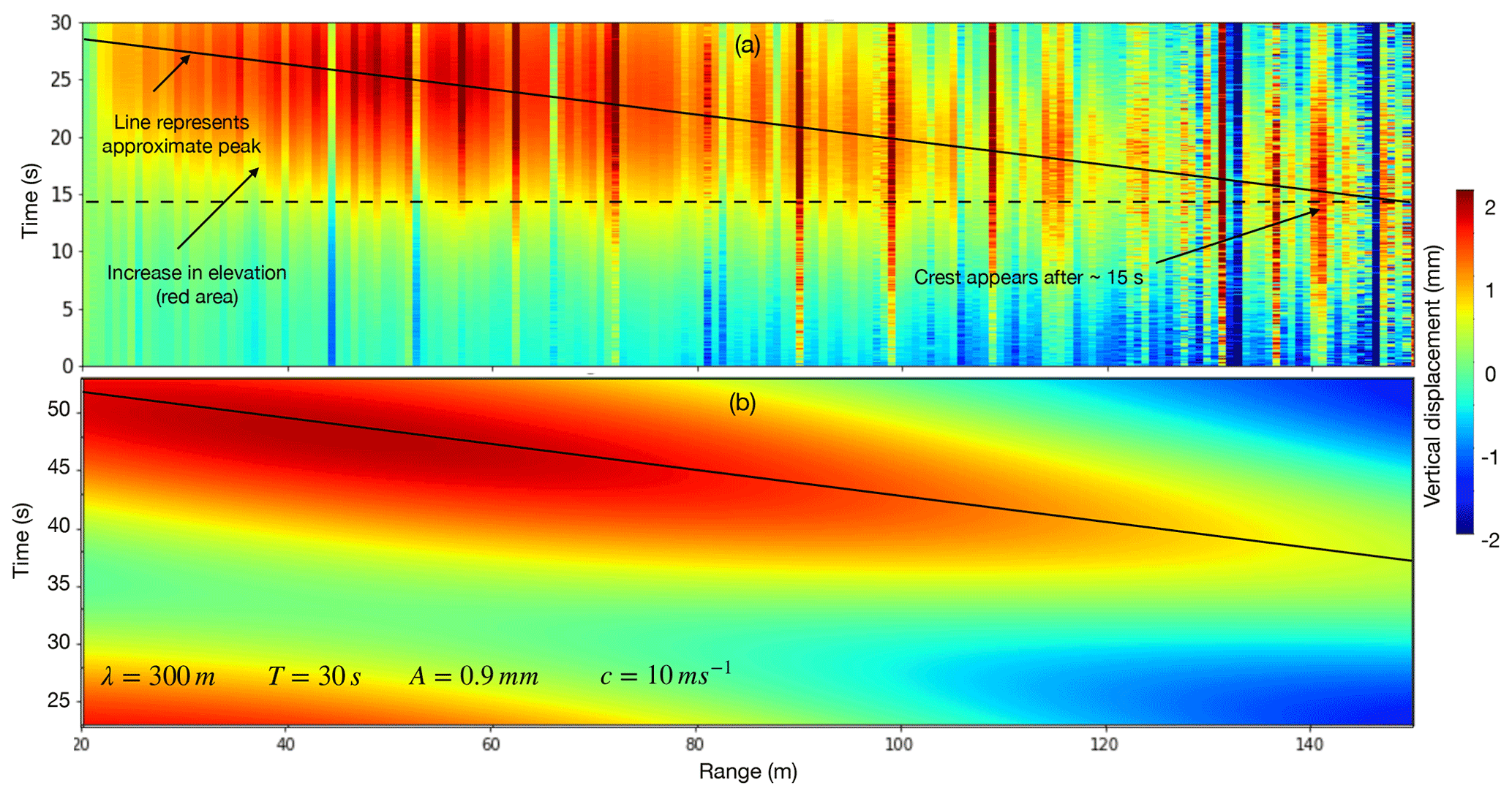
Figure 5(a) Phase-derived vertical displacement over 30 s at 21:56 UTC. The displacement is displayed in the range-time space along one fixed direction. Transient features are thus expected to have a diagonal nature, where the angle represents the velocity of the feature. (b) Modeled displacement of a similar wave as in panel (a).
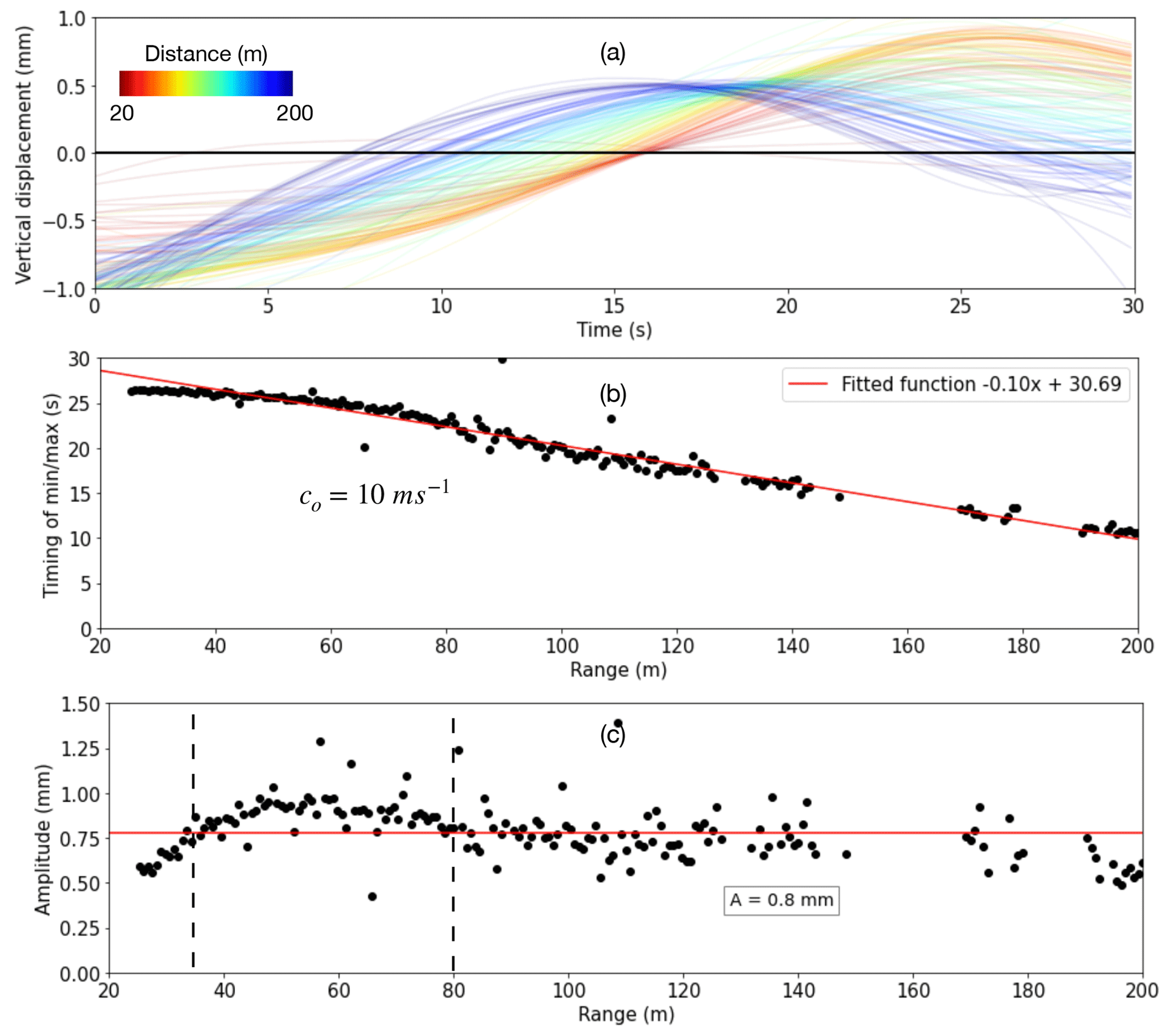
Figure 6(a) Derived vertical displacement over 30 s on 23 April 2021 at 21:56 UTC (E1). Each line represents one location on the ice, where warmer colors signify a distance closer to the radar. (b) Exact time of the wave crest at different distances from the radar. The linear fit indicates a wave velocity of 10.0 m s−1. (c) Amplitude with range.
3.2 Observing superimposed wave fields validated with data from Ice Wave Riders
The three Ice Wave Riders (IWR) were continuously operating from approximately 00:30 UTC on 24 April (Table 1), overlapping two GPRI acquisitions in the offshore direction. The derived vertical displacement is thus suitable for validation of the GPRI data acquired at 00:32 and 00:44 UTC on 24 April. In this time window, we determine a cross-correlation lag time of l=63.5 s in between IWRs, indicative of predominately onshore wave propagation (Eq. 8). We further evaluate the displacement spectral characteristics in the Welch periodograms (Fig. 7). Wave amplitude relates to frequency according to Eq. (9), resulting in the lower frequencies in Fig. 4 dominating the displacement (Fig. 7). The displacement exhibits energetic signals between 30 and 60 s, well within the wave band for flexural waves, which persist for less than an hour. Both IWR 33 and IWR 34 suggest that several of the frequency peaks during and following the GPRI acquisitions (red line in Fig. 7) are centered around 43 s (black lines in Fig. 7). Although these peaks are small with an amplitude of ∼ 1 cm, they are significantly above the derived noise floor as indicated in Fig. 8. IWR 35 is situated behind grounded ice, in shallower water with thicker ice, and does not exhibit the same signal as the other IWRs.
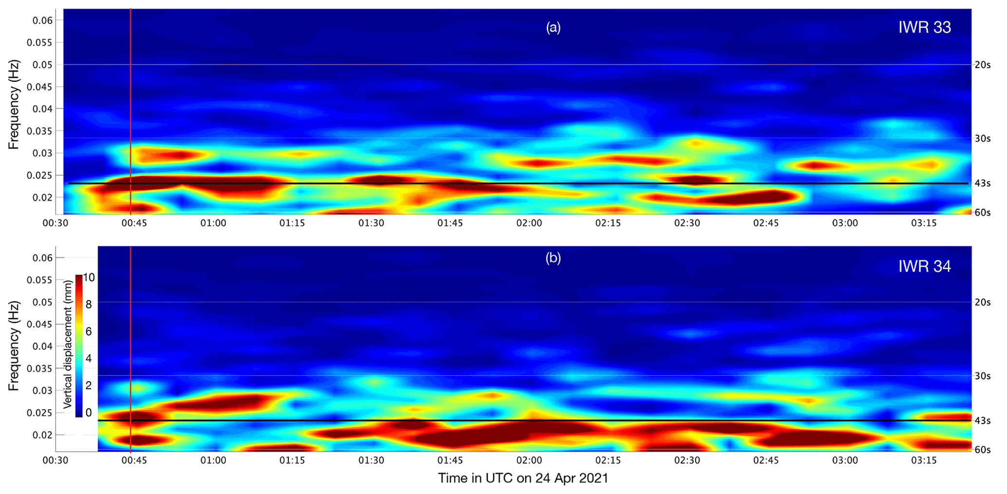
Figure 7Spectra of the wave amplitude computed from the vertical acceleration from IWR 33 (Fig. 4) and from IWR 34 presented as ∼ 3 h Welch plots from 24 April 2021. The displacement of IWR 33 is centered on a period of 43 s (black lines) at 00:44 UTC (time indicated with vertical red line).
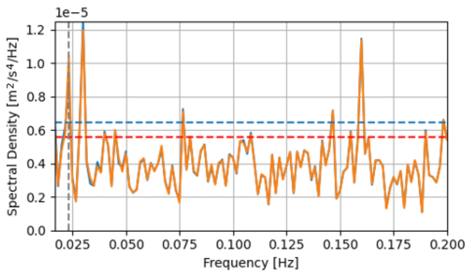
Figure 8Solid lines indicate raw (blue) and bandpass-filtered (orange) spectral density during the first hour of the IWR record. Dashed red line indicates the noise floor of the IMU sensor (from the VectorNav data sheet). Dashed blue line indicates the noise floor derived from the IWR when resting on the floor. The 43 s wave signal at ∼ 0.025 Hz exceeds both of these noise floors.
The last of the GPRI interferograms acquired at 00:44 UTC (referred to as E2) exhibits a clean wave-like motion (Fig. 9a). We are able to track the timing of displacement maximums and minimums across most of the lead (Fig. 9b) with a temporal lag of 21.4 ± 0.5 s. The period is exactly double at T=42.7 ± 1.0 s. This corresponds to the peak displacement frequency derived from IWR 33 (within the measurement uncertainty) and suggests that the GPRI picks up the same wave field. The observed wave speed, derived from the slope of the maximum ice displacement (Fig. 9b), is 27 m s−1 (with a standard error of 25 cm s−1) and larger than the speed of the incoming wave field at 10 m s−1. We therefore assume that the observations represent a reflected edge wave that can propagate along the lead superimposed on the incoming wave field identified with the IWRs. The actual speed of the two wave fields will be 10 m s−1, but the observed speed of the edge wave, co2, needs to be considered. The reflected wave will have a conserved period, T, and the same is the case for the superimposed waves as demonstrated in Fig. 3b. As described by Eq. (7), m s−1 results in co2 = 44 m s−1 and suggests wave propagation at ∼ 76∘ from the LOS. This is indicative of an edge wave traveling directly up the refrozen lead (pink dashed line in Fig. 1b).
In addition to waves reflecting at ice boundaries and traversing along leads and ridges at an angle, we expect the incoming wave field to also be able to reflect directly off the iceberg with a conserved orientation. This is expected to lead to a standing wave as modeled in Fig. 3c. A possible example of this was observed prior to the IWR data (Fig. 10), where the minimum elevation of the trough occurs at ∼ 15 s out to a node of 100 m and beyond at ∼ 27.5 s, indicative of a standing wave with T≈25 s. However, this signal bearing a resemblance to a standing wave does not indicate more nodes (e.g., at ∼ 300 m) and incorporates a linear trend that was removed for the analysis (dashed line in Fig. 10). This could be due to a simultaneous increase in water level or a superimposed lower-frequency wave field.
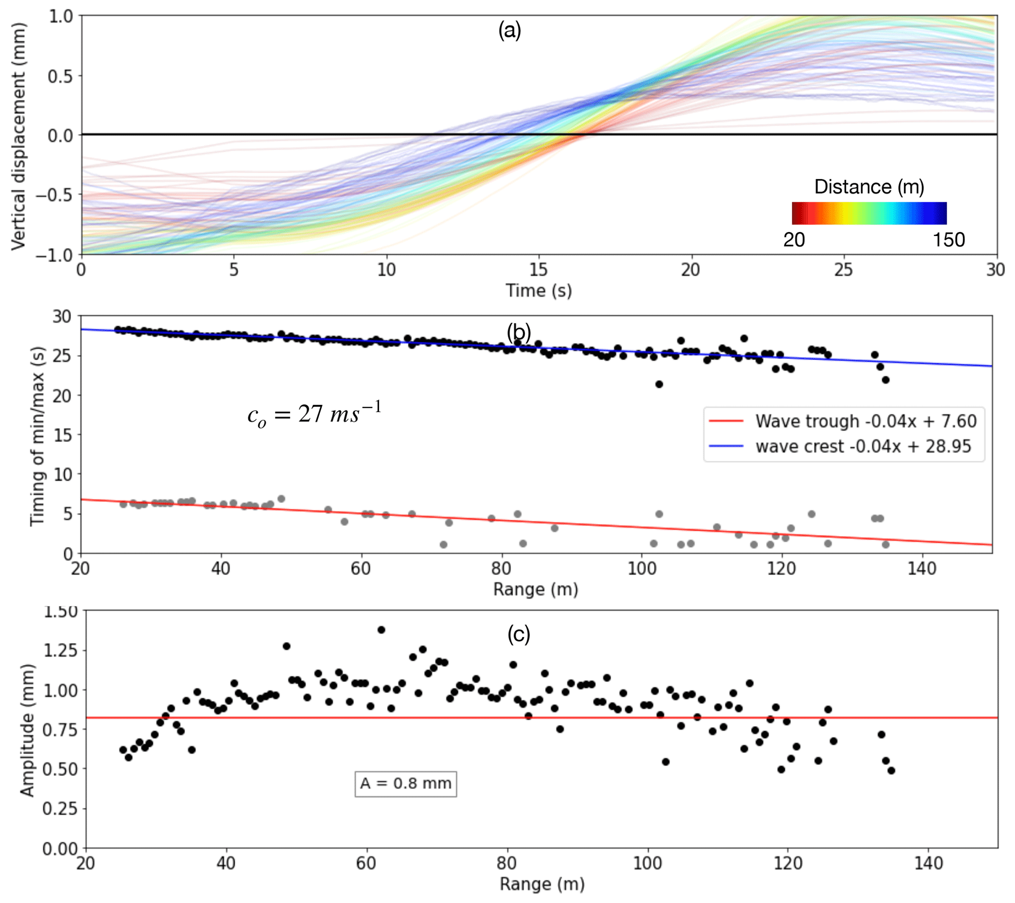
Figure 9(a) Derived vertical displacement over 30 s on 24 April 2021 at 00:44 UTC (E2). Each line represents one location on the ice, where warmer colors signify a distance closer to the radar. (b) Exact time of the wave crest and troughs at different distances from the radar. The linear fit indicates a wave velocity of 27 m s−1 and period of 43 s. (c) Amplitude with range.
4.1 Interpreting wave amplitude and speed
The wave amplitudes derived from GPRI stare-mode observations approximately 3 h apart (E1 and E2) are similar to each other and peaks at ∼ 60–80 m from the GPRI. Offshore from this distance, we attribute the increase in amplitude to shoaling as the water gets shallower. Closer than ∼ 60 m from the GPRI, the wave amplitude drops by nearly 50 % in both instances. A possible explanation for this is the presence of deformed, thicker ice near the GPRI (small picture in Fig. 1a) and mechanical coupling between the floating sea ice and grounded iceberg.
The average observed speed in E1 matches well with the shallow-water approximation indicative of an onshore wave. However, the speed appears to increase within ∼ 70 m of the GPRI, which is apparent as a flattening of the curve representing the timing of the wave maximums (Fig. 6b). One possible explanation is deflection as the wave approaches the grounded ice giving the appearance of higher speed due to a larger angle between propagation and LOS. Another possible explanation is that the ice in the near range is not in hydrostatic equilibrium and hence reaches its maximum value quicker than when the actual wave crest arrives. A third explanation is that the wave reflects off the grounded ice, resulting in a maximum ice displacement which differs from the wave crest. The latter two explanations are based on the fact that the speed is strictly derived from the displacement maximum, which may not represent the wave crest and thus may lead to inaccuracies.
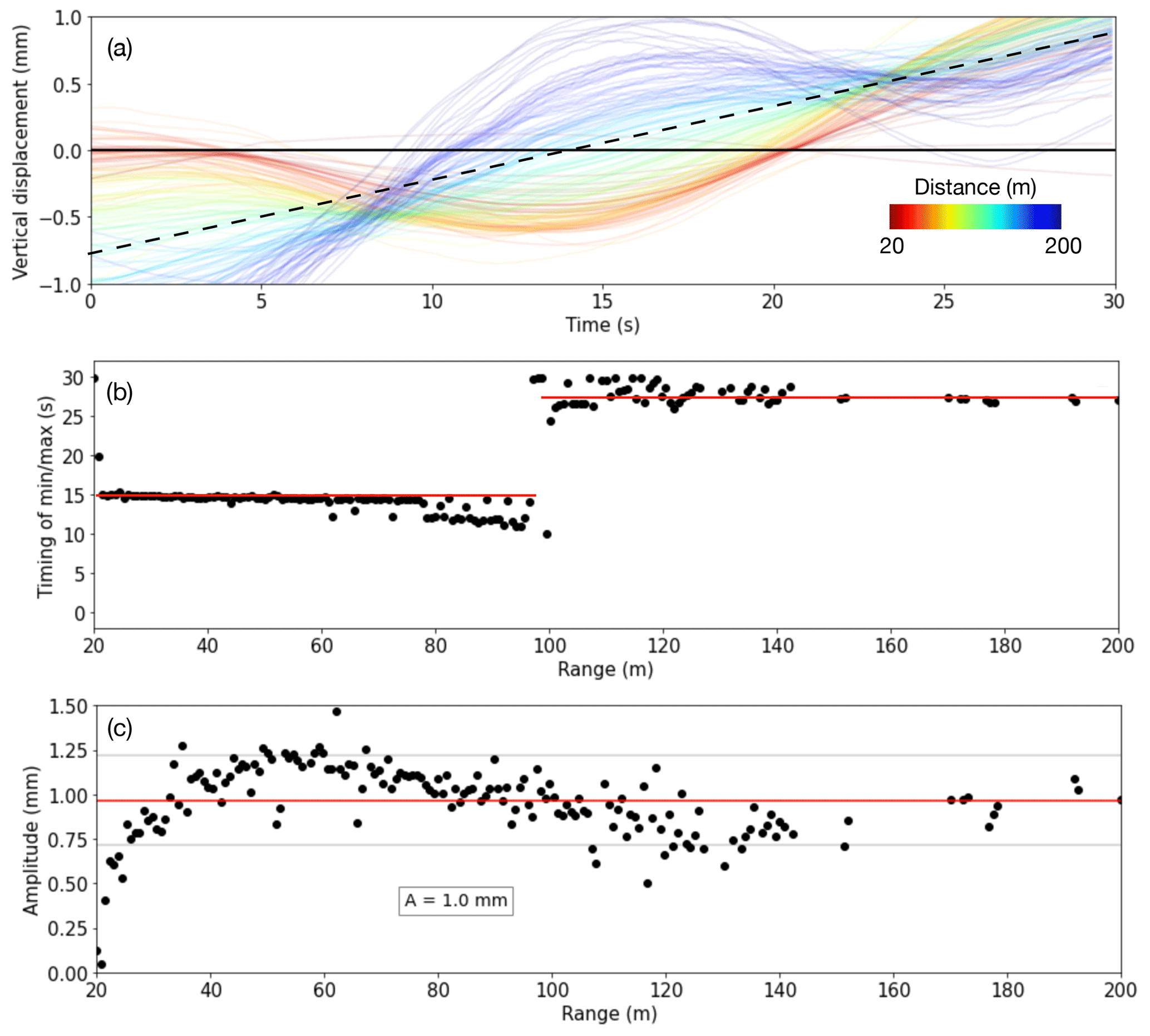
Figure 10(a) Derived vertical displacement over 30 s on 23 April 2021 at 22:32 UTC (E2). Each line represents one location on the ice, where warmer colors signify a distance closer to the radar. The dashed line indicates a linear trend removed for the analysis. (b) Exact time of the trough at different distances from the radar. The red lines indicate average values on each side of the node. (c) Amplitude with range with the red line indicating the mean.
4.2 Uncertainties related to propagation angle and amplitude
The average observed speed in E2 is 27 m s−1, 17 m s−1 higher than during E1. One possible explanation for this is the presence of an edge wave traveling at an angle ∼ 76∘ from LOS. Although we expect incoming waves to typically orient onshore, such waves can excite waves in ice discontinuities with a conserved period, which will propagate along such boundaries (Marchenko and Semenov, 1994; Marchenko, 1999; Evans and Porter, 2003). We speculate that E2 may incorporate one of these edge waves generated at the boundary between the refrozen lead and offshore ice (green arrow in Fig. 1b). The wave then propagates along this boundary directly up the refrozen lead (dashed pink line in Fig. 1b). A second explanation is the stark inhomogeneities in the ice, such as fractures, variable thickness, and rough ice leading to significant reorientation of the wave. InSAR-based (interferometric synthetic-aperture radar) snapshots of infragravity wave fields in sea ice indicate that waves fronts can be reorientated by tens of degrees by spatial variations in bathymetry and ice morphology (Mahoney et al., 2016).
The wave amplitude in E2 differs from what was observed with the IWRs by an order of magnitude. This is not necessarily surprising as the GPRI was not staring directly at any of the IWRs and satellite-based InSAR observations suggest significant variation in vertical motion (even featuring locations of negligible motion) along a single wave front (Mahoney et al., 2016). Hence, in inhomogeneous ice, vertical displacement should be expected to significantly deviate from the average amplitude. Furthermore, if the E2 wave represents a generated edge wave, this may also have resulted in a diminished amplitude value in addition to attenuation and bathymetric influence on the amplitude. In essence, we do not observe nor expect the amplitude to be conserved in between the well-separated IWRs and the GPRI in the same way as the wave period. The derived amplitude is dependent upon the incidence angle, θ, which is subject to uncertainties, predominately driven by inexact estimation of the antenna height atop of the iceberg. Uncertainties from sensor tilt due to iceberg motion are not considered, as tilt could be identified in the antenna leveler and interferometric phase as illustrated in Appendix A.
4.3 Interpretation constraints due to multiple wave fields and horizontal motion
In addition to E1 and E2, many other examples exhibit wave-like motion in the GPRI data (see the Supplement) but can be challenging to interpret partly due to the presence wave fields with different sources and frequencies as well as horizontal motion. The IWR data suggest that essentially all frequencies in between 0.15–0.02 Hz can occur in the ice and multiple frequencies can be present at one time (Fig. 4). The separation of multiple wave signals is challenging due to the short 30 s acquisition window, resulting in the predominate capture of partial waves.
In addition to the interpretation challenges from multiple frequency signals, ice displacement in the horizontal plane appears to be the most common limitation for wave interpretation due to frequent horizontal ice motion. The GPRI is more sensitive to horizontal movement than to an equal displacement in the vertical direction. Hence, even modest lateral motion can complicate wave interpretation. This sensitivity may also enable the GPRI to potentially detect compressional or shear waves from ice–ice interaction propagating in the horizontal plane. However, such waves propagate at speeds on the order of kilometers per second (Rajan et al., 1993) and is expected to result in sharp peaks in displacement that may be difficult to detect. Even though horizontal movement often complicates interpretation, it can typically be identified in a phase signal. This is due to the low vertical sensitivity with range that can lead to implausible values if interpreted as vertical (Dammann et al., 2021b) and the observed identical timing of displacement peaks with range.
This work leverages data from a 2021 coordinated GPRI–IWR campaign to demonstrate and validate the capture of flexural–gravity waves by the two sensors. The GPRI data were captured during modest wave activity <∼ 1 mm, and less than ∼ 5 % of acquisitions could be used to interpret wave properties due to the presence of what we interpret to be horizontal surface motion and interfering wave fields. We expect this percentage to be larger if data are acquired during larger-amplitude and more persistent wave activity. However, two particularly clear examples analyzed here demonstrate the ability to track waves with amplitudes of 1 mm and properties over 100–200 m during the absence of secondary motion.
We also expect the collection of longer time series to aid the interpretation in the future. In this work we were limited to 30 s of continuous radar acquisitions due to system constraints in stare mode, specifically the data-writing speed of the specific version of the GPRI hardware used here. This limitation does not extend to newer GPRI systems, enabling continuous stare-mode acquisitions over hours to potentially days. This will open up possibilities for a more thorough evaluation of the wave signal. For instance, where we are here limited to look for single “clean” individual waves, we will be able to analyze combinations of multiple waves and frequencies for instance by applying Fourier analysis.
While the IWRs and similar on-ice installments enable the detection of waves and their properties, the GPRI provides the ability to spatially track individual waves. In addition to identifying the wave period, speed, and amplitude, it can possibly help provide insight into how these properties change over a few hundred meters as a result of variations in the ice cover. Coordinated GPRI–IWR deployments can be particularly useful as they can resolve both regional variability in wave activity as well as the tracking of individual waves in select locations. Future deployments could attempt to place an IWR directly in LOS with the GPRI to derive properties of the same wave with both sensors to investigate and resolve potential inconsistencies.
While the results discussed here show promise, the acquisition of longer time series and different types of waves is required to investigate potential applications. In this work, we analyzed infragravity waves, but the GPRI, with its high measurement frequency, can likely determine wave properties of ocean swells that can lead to ice fracture and destabilization. For ice subject to break out, the GPRI is particularly valuable as it does not require deployment on the ice. Furthermore, the GPRI and the IWRs can provide near-real-time data not available from other instruments (e.g., moorings) and can potentially aid in the development of an early warning system for ice breakout.
Waves will impact ΔΦ in different ways depending on whether the GPRI is stationed on moving ice or a fixed surface. In the case of a GPRI placed on floating ice that moves with the waves, the relative vertical displacement, , has an additional component due to the vertical motion of the antenna:
This second term is equivalent to dv evaluated at x=0 (red line in Fig. A1a). As the waves propagate underneath the GPRI, the antenna will also be subjected to a variable tilt angle, ε, depending on the amplitude, A, and wavelength, λw:
This will lead to periodic horizontal motion, (blue line in Fig. A1a), depending on the elevation of the GPRI antenna, h:
The resulting interferogram from both and (Fig. A1b) has similarities to interferograms from a fixed system (Fig. 2) but is more challenging to interpret (e.g., derive wave speed) due to the added complexity.
To highlight the contributions from vertical and horizontal motion to the phase for a floating GPRI, we isolate the relative vertical motion, , in Fig. A2a. At distances equal to multiples of the wavelengths (), the GPRI and the ice surface will move in phase, leading to nodes where (Fig. A2a). Halfway between these nodes (), the GPRI and ice surface will move out of phase, leading to a maximum relative vertical displacement twice that of the wave amplitude. Similarly, in Fig. A2b we isolate the much smaller component of periodic horizontal motion, . The resulting interferogram from exhibits a predominate near-range phase response, while the interferogram due to exhibits a phase contribution nearly independent of range (Fig. A2c and d respectively). The effect of Fig. A2c and d results in the interferogram in Fig. A1b.
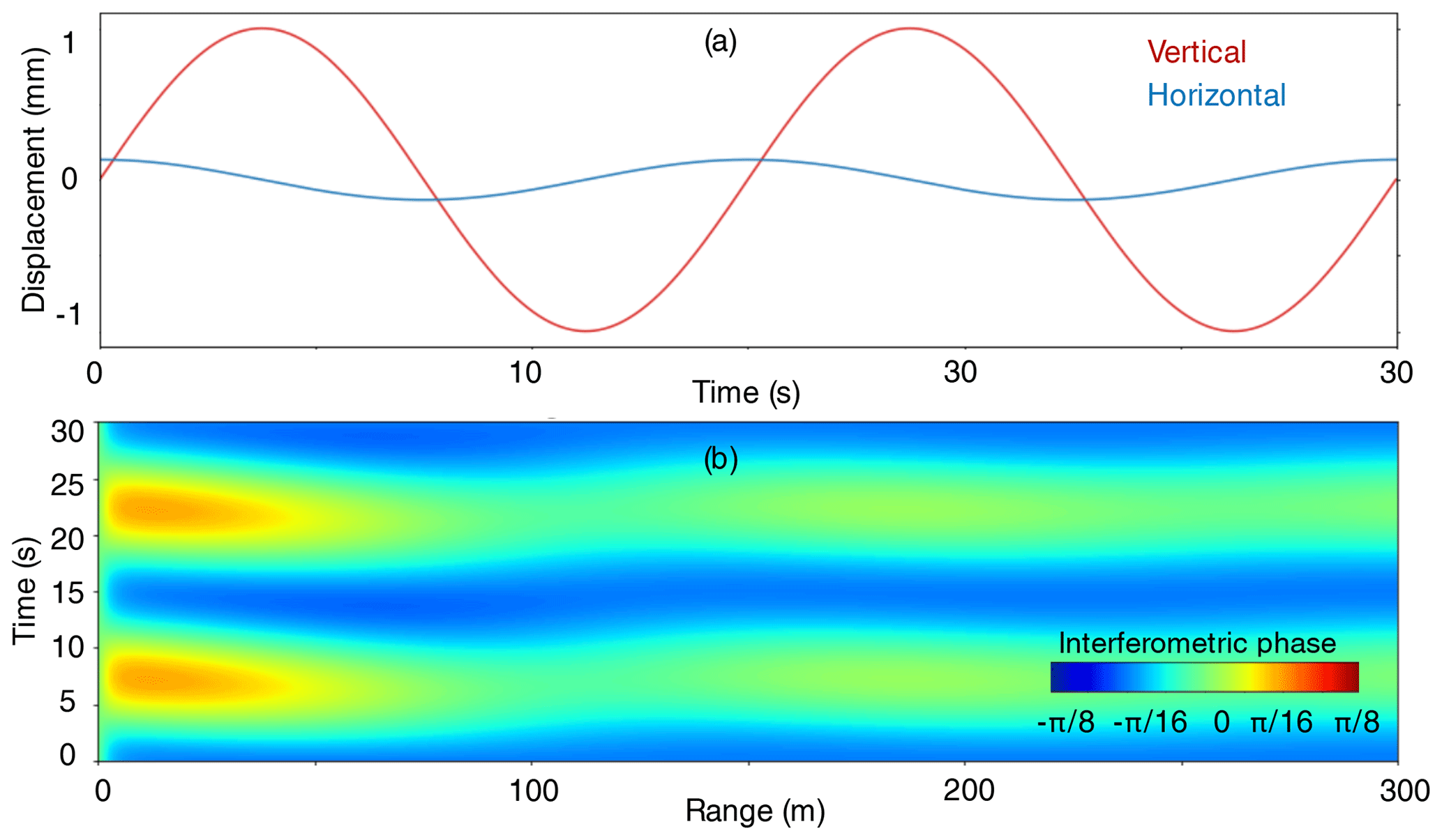
Figure A1(a) Simulated vertical (red) and horizontal (blue) GPRI antenna motion as a result of waves (T=15 s, A=1 mm, λw=150 m, h=2 m). (b) Simulated interferogram of a floating GPRI system based on a propagating wave including antenna motion in panel (a).
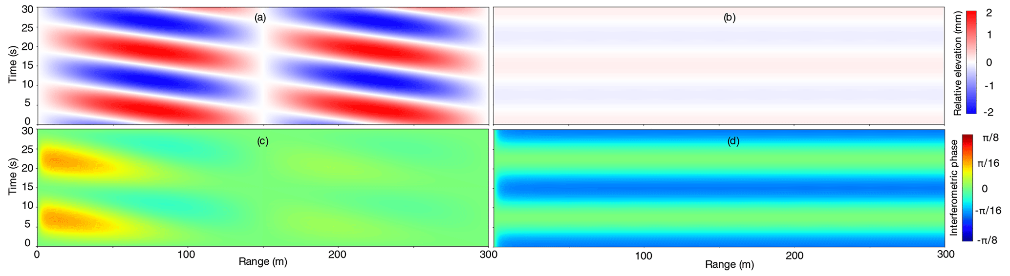
Figure A2Relative change in the (a) vertical and (b) horizontal distance between the GPRI antenna and the ice surface due to the wave in Fig. A1. Panels c and d represent the resulting interferograms from the isolated motion in panels (a) and (b).
Code can be made available upon request.
Data can be made available upon request.
The supplement related to this article is available online at: https://doi.org/10.5194/tc-17-1609-2023-supplement.
DOD conducted the interferometric processing and analysis and drafted the initial manuscript. MAJ contributed to all aspects of the analysis and manuscript. ARM and ERF designed the field experiment, collected the data, and provided critical guidance on data interpretation. All co-authors provided valuable recommendations and corrections resulting in the final manuscript.
The contact author has declared that none of the authors has any competing interests.
Publisher's note: Copernicus Publications remains neutral with regard to jurisdictional claims in published maps and institutional affiliations.
We thank Alexey Marchenko at the University Centre in Svalbard (UNIS) for valuable discussions on wave propagation in sea ice. We thank Matthew Druckenmiller at the National Snow and Ice Data Center (NSIDC) for providing ice thickness data. We are grateful to personnel at Ukpeaġvik Iñupiat Corporation (UIC) Science for logistical support. We thank Alexey Marchenko again, Jim Thomson, and Marcel Kleinherenbrink for a thorough review which significantly improved this paper.
This research has been supported by the Office of Naval Research (grant no. N000141912451) and the U.S. Army Corps of Engineers (grant no. W913E521C0004).
This paper was edited by Lars Kaleschke and reviewed by Aleksey Marchenko, Jim Thomson, and Marcel Kleinherenbrink.
Ardhuin, F., Collard, F., Chapron, B., Girard-Ardhuin, F., Guitton, G., Mouche, A., and Stopa, J. E.: Estimates of ocean wave heights and attenuation in sea ice using the SAR wave mode on Sentinel-1A, Geophys. Res. Lett., 42, 2317–2325, https://doi.org/10.1002/2014GL062940, 2015.
Ardhuin, F., Stopa, J., Chapron, B., Collard, F., Smith, M., Thomson, J., Doble, M., Blomquist, B., Persson, O., and Collins III, C. O.: Measuring ocean waves in sea ice using SAR imagery: A quasi-deterministic approach evaluated with Sentinel-1 and in situ data, Remote Sens. Environ., 189, 211–222, https://doi.org/10.1016/j.rse.2016.11.024, 2017.
Bromirski, P. D., Sergienko, O. V., and MacAyeal, D. R.: Transoceanic infragravity waves impacting Antarctic ice shelves, Geophys. Res. Lett., 37, L02502, https://doi.org/10.1029/2009GL041488, 2010.
Bromirski, P. D., Diez, A., Gerstoft, P., Stephen, R. A., Bolmer, T., Wiens, D., Aster, R., and Nyblade, A.: Ross ice shelf vibrations, Geophys. Res. Lett., 42, 7589–7597, https://doi.org/10.1002/2015GL065284, 2015.
Collard, F., Marié, L., Nouguier, F., Kleinherenbrink, M., Ehlers, F., and Ardhuin, F.: Wind-Wave Attenuation in Arctic Sea Ice: A Discussion of Remote Sensing Capabilities, J. Geophys. Res.-Oceans, 127, e2022JC018654, https://doi.org/10.1029/2022JC018654, 2022.
Crocker, G. and Wadhams, P.: Observations of wind-generated waves in Antarctic fast ice, J. Phys. Oceanogr., 18, 1292–1299, https://doi.org/10.1175/1520-0485(1988)018<1292:OOWGWI>2.0.CO;2, 1988.
Czipott, P. V. and Podney, W. N.: Measurement of fluctuations in tilt of Arctic ice at the Cearex Oceanography Camp: experiment review, data catalog and preliminary results, La Jolla, CA, Physical Dynamics Inc. (Phys. Dyn. Tech. Rep. PD-LJ-89-369R.), 1989.
Dammann, D. O., Johnson, M. A., Fedders, E., Mahoney, A., Werner, C., Polashenski, C. M., Meyer, F., and Hutchings, J. K.: Ground-based radar interferometry of sea ice, Remote Sensing, 13, 43, https://doi.org/10.3390/rs13010043, 2021a.
Dammann, D. O., Mahoney, A., Johnson, M., Eicken, H., Eriksson, L. E. B., Meyer, F., Fedders, E., and Fahnestock, M.: Applications of radar interferometry for measuring ice motion, in: Proceedings of the 26th International Conference on Port and Ocean Engineering under Arctic Conditions, Moscow, Russia, 14–18 June 2021, https://www.poac.com/Proceedings/2021/POAC21-012.pdf (last access: 6 April 2023), 2021b.
Dammann, D. O., Johnson, M. A., Mahoney, A., Fedders, E., Ito, M., Hutchings, J. K., Polashenski, C. M., and Fahnestock, M.: Ground-based radar interferometry for monitoring landfast sea ice dynamics, Cold Reg. Sci. Technol., 210, 103779, https://doi.org/10.1016/j.coldregions.2023.103779, 2023.
Doble, M., Mercer, D. J., Meldrum, D., and Peppe, O. C.: Wave measurements on sea ice: developments in instrumentation, Ann. Glaciol., 44, 108–112, https://doi.org/10.3189/172756406781811303, 2006.
Druckenmiller, M. L., Eicken, H., George, J. C., and Brower, L.: Trails to the whale: reflections of change and choice on an Iñupiat icescape at Barrow, Alaska, Polar Geography, 36, 5–29, https://doi.org/10.1080/1088937X.2012.724459, 2013.
Evans, D. and Porter, R.: Wave scattering by narrow cracks in ice sheets floating on water of finite depth, J. Fluid Mech., 484, 143–165, https://doi.org/10.1017/S002211200300435X, 2003.
Horvat, C., Blanchard-Wrigglesworth, E., and Petty, A.: Observing waves in sea ice with ICESat-2, Geophys. Res. Lett., 47, e2020GL087629, https://doi.org/10.1029/2020GL087629, 2020.
Johnson, M., Mahoney, A., Sybrandy, A., and Montgomery, G.: Measuring acceleration and short-lived motion in landfast sea-ice, J. Ocean Technol., 15, 115–131, https://www.thejot.net/article-preview/?show_article_preview=1190 (last access: 6 April 2023), 2020.
Johnson, M. A., Marchenko, A. V., Dammann, D. O., and Mahoney, A. R.: Observing Wind-Forced Flexural-Gravity Waves in the Beaufort Sea and Their Relationship to Sea Ice Mechanics, Journal of Marine Science and Engineering, 9, 471, https://doi.org/10.3390/jmse9050471, 2021.
Kohout, A. L., Penrose, B., Penrose, S., and Williams, M. J.: A device for measuring wave-induced motion of ice floes in the Antarctic marginal ice zone, Ann. Glaciol., 56, 415–424, https://doi.org/10.3189/2015AoG69A600, 2015.
Kovalev, D. P., Kovalev, P. D., and Squire, V. A.: Crack formation and breakout of shore fast sea ice in Mordvinova Bay, south-east Sakhalin Island, Cold Reg. Sci. Technol., 175, 103082, https://doi.org/10.1016/j.coldregions.2020.103082, 2020.
Kovalev, P. D. and Squire, V. A.: Ocean wave/sea ice interactions in the south-eastern coastal zone of Sakhalin Island, Estuarine, Coastal and Shelf Science, 238, 106725, https://doi.org/10.1016/j.ecss.2020.106725, 2020.
Mahoney, A., Dammann, D. O., Johnson, M. A., Eicken, H., and Meyer, F. J.: Measurement and imaging of infragravity waves in sea ice using InSAR, Geophys. Res. Lett., 43, 6383–6392, https://doi.org/10.1002/2016GL069583 2016.
Marchenko, A.: Parametric excitation of flexural-gravity edge waves in the fluid beneath an elastic ice sheet with a crack, Eur. J. Mech. B-Fluid., 18, 511–525, https://doi.org/10.1016/S0997-7546(99)80046-6, 1999.
Marchenko, A. and Semenov, A. Y.: Edge waves in a shallow fluid beneath a fractured elastic plate, Fluid Dyn., 29, 589–592, https://doi.org/10.1007/BF02319083, 1994.
Rabault, J., Sutherland, G., Gundersen, O., Jensen, A., Marchenko, A., and Breivik, Ø.: An open source, versatile, affordable waves in ice instrument for scientific measurements in the Polar Regions, Cold Reg. Sci. Technol., 170, 102955, https://doi.org/10.1016/j.coldregions.2019.102955, 2020.
Rajan, S. D., Frisk, G. V., Doutt, J. A., and Sellers, C. J.: Determination of compressional wave and shear wave speed profiles in sea ice by crosshole tomography – Theory and experiment, J. Acoust. Soc. Am., 93, 721–738, https://doi.org/10.1121/1.405436, 1993.
Smith, M. and Thomson, J.: Pancake sea ice kinematics and dynamics using shipboard stereo video, Ann. Glaciol., 61, 1–11, https://doi.org/10.1017/aog.2019.35, 2020.
Squire, V. A.: An investigation into the use of strain rosettes for the measurement of propagating cyclic strains, J. Glaciol., 20, 425–431, https://doi.org/10.3189/S0022143000013952, 1978.
Squire, V. A.: Of ocean waves and sea-ice revisited, Cold Reg. Sci. Technol., 49, 110–133, https://doi.org/10.1016/j.coldregions.2007.04.007, 2007.
Squire, V. A.: A fresh look at how ocean waves and sea ice interact, Philos. T. R. Soc. A, 376, 20170342, https://doi.org/10.1098/rsta.2017.0342, 2018.
Squire, V. A., Dugan, J. P., Wadhams, P., Rottier, P. J., and Liu, A. K.: Of ocean waves and sea ice, Annu. Rev. Fluid Mech., 27, 115–168, 1995.
Sutherland, G. and Rabault, J.: Observations of wave dispersion and attenuation in landfast ice, J. Geophys. Res.-Oceans, 121, 1984–1997, https://doi.org/10.1002/2015JC011446, 2016.
Sutherland, P., Brozena, J., Rogers, W. E., Doble, M., and Wadhams, P.: Airborne remote sensing of wave propagation in the marginal ice zone, J. Geophys. Res.-Oceans, 123, 4132–4152, https://doi.org/10.1029/2018JC013785, 2018.
Thomson, J. and Rogers, W. E.: Swell and sea in the emerging Arctic Ocean, Geophys. Res. Lett., 41, 3136–3140, https://doi.org/10.1002/2014GL059983, 2014.
Thomson, J., Gemmrich, J., Rogers, W. E., Collins, C. O., and Ardhuin, F.: Wave groups observed in pancake sea ice, J. Geophys. Res.-Oceans, 124, 7400–7411, https://doi.org/10.1029/2019JC015354, 2019.
Yadav, J., Kumar, A., and Mohan, R.: Dramatic decline of Arctic sea ice linked to global warming, Nat. Hazards, 103, 2617–2621, https://doi.org/10.1007/s11069-020-04064-y, 2020.