Brief communication: Mountain permafrost acts as an aquitard during an infiltration experiment monitored with electrical resistivity tomography time-lapse measurements

Frozen layers within the subsurface of rock glaciers are generally assumed to act as aquicludes or aquitards. So far, this behavior has been mainly defined by analyzing the geochemical characteristics of spring waters. In this work, for the first time, we experimentally confirmed this assumption by executing an infiltration test in a rock glacier of the Southern Alps, Italy. Time-lapse electrical resistivity tomography (ERT) technique monitored the infiltration of 800 L of saltwater released on the surface of the rock glacier; 24 h ERT monitoring highlighted that the injected water was not able to infiltrate into the underlying frozen layer.

1 Introduction

In alpine regions, groundwater originating from moraines and rock glaciers highly contributes to the streamflow (Wagner et al., 2016). Therefore, a key factor in the hydrological modeling of alpine catchments is the determination of the hydraulic properties of these landforms. The subsoil hydrodynamic of moraines, talus and hillslope aquifers is relatively well known, but the hydraulic behavior of rock glaciers and their impact on the hydrology of alpine catchments are relatively less defined (Pauritsch et al., 2017, and references therein). The hydrological and geochemical monitoring of active rock glaciers springs was successfully used to investigate runoff processes and presence of frozen layer in alpine catchments (e.g., Krainer et al., 2007; Carturan et al., 2016). In active or ice-rich intact rock glaciers, continuous frozen layers are typically considered aquicludes (Giardino et al., 1992). Krainer et al. (2007) separated a subsurface flow component, derived from snow–ice melting and rainwater, and a deeper and longer stored aquifer at the bottom of the Reichenkar active rock glacier (Austrian Alps). Harrington et al. (2018) defined the inactive Helen Creek rock glacier (Alberta, Canada) as an unconfined aquifer, as the limited ground ice distribution is unlikely to act as a pure aquiclude. These investigations suggest that rock glaciers host complex and heterogeneous aquifers with a layered internal structure. Nevertheless, geochemical surveys do not have the ability to accurately define the aquifer's structure (e.g., layer thickness, discontinuities and lateral/vertical heterogeneities) if not integrated with geophysical surveys.

To verify and confirm the hydraulic behavior of the frozen layer, we tested an infiltration experiment combined with electrical resistivity tomography (ERT) time-lapse measurements in the Sadole rock glacier (Southern Alps, Italy). Controlled irrigation experiments combined with ERT time-lapse measurements were successfully applied to study the vadose zone (Cassiani et al., 2016) and even more challenging hillslope catchments (Cassiani et al., 2009). The Sadole rock glacier infiltration experiment represents the first attempt to adopt this monitoring technique to the mountain permafrost environment. Considering the promising results, the experiment can be used as a reference to improve future tests and better characterize the hydraulic properties of the frozen subsoils.

2 Site description

The Sadole rock glacier is located in the Sadole Valley, in the eastern part of the province of Trento (northeastern Italy, Fig. 1a). The rock glacier altitude ranges between 1820 and 2090 m a.s.l. It is a complex periglacial landform made by the confluence of three different lobes (Fig. 1b), which developed on two coalescent glacial cirques. Steep rock walls and sharp crests almost entirely bound these cirques, except for the Sadole Pass, which was likely a glacial transfluence saddle during the last glaciation. Slope deposits are found between the rock walls and the rock glacier rooting areas. These deposits have gravitational or mixed gravitational–debris-flow–avalanche origin and are predominantly active. From a geological point of view, the rock glacier is composed of magmatic rocks (riodacitic ignimbrites) that belong to the Athesian Volcanic Group, a late-Paleozoic (Permian) volcanic succession. The Sadole rock glacier is classified as a “relict” in the inventory of the province of Trento (Seppi et al., 2012), in agreement with the guidelines provided by the IPA Action Group (RGIK, 2022). Despite this, the general convex morphology and the low water temperature of its springs (ranging between 1.0 and 1.8 ^∘C) suggested that this rock glacier may preserve permafrost (Carturan et al., 2016, and references therein). In addition, ice outcrops were observed in the mid-summer 2 m below the surface, in a pit dug during World War I (green dot in Fig. 1b). Several ERT transects (blue, violet and brown lines in Fig. 1b) were collected in summer 2021 on the rock glacier, confirming the presence of a discontinuous frozen layer (see high resistivity areas in Fig. 1d–e). Soil temperature sensors (red dots in Fig. 1b) were installed in different location of the rock glacier bodies. Finally, to evaluate the hydraulic behavior of the frozen layer, an infiltration experiment with ERT time-lapse measurements was realized in middle June 2022. The ERT monitoring transect (red line in Fig. 1c) was in the same area of the ERT surveys in 2021, considering the maximum slope gradient. The line was placed to detect how the injected water flows in the area where the frozen layer is present and how it flows where the frozen layer ends.

Figure 1 (a) Geographic location of the Sadole rock glacier (yellow star), adapted from © Google Earth Pro and Italian Physical Map produced by The University of Texas at Austin; (b) hillshade lidar DEM (modified from WebGIS PAT – Provincia Autonoma di Trento) showing the three different units that compose the Sadole rock glacier (yellow lines). Blue, violet and brown lines represent ERT surveys performed in summer 2021; red circles define the position of soil temperature sensors, and the green circle is the location of the Austrian well (World War I); (c) orthophoto (produced by Commissione Glaciologica SAT, 2022) showing the ERT transect (red line) used for the infiltration experiment, the saltwater injection point (blue star – 1950 m a.s.l.), and the location of the rock glacier spring (brownish triangle – 1796 m a.s.l.). Blue and violet dashed lines represent ERT surveys performed in 2021 and showed at a larger scale in Fig. 1b. (d) Inverted resistivity section of the blue ERT survey line performed in summer 2021. (e) Inverted resistivity section of the violet ERT survey line performed in summer 2021.

3 Methods

3.1 Experiment principles

ERT surveys are performed to detect the electrical properties of the ground. The method can be used for monitoring time-dependent subsurface processes by repeating periodically the measurements using the same electrode array (Binley, 2015). This ERT data acquisition method is defined as “ERT time-lapse technique” and can be performed with controlled irrigation experiments (Cassiani et al., 2006, 2009). In these tests, a large amount of saltwater is released into the subsoil system, and the propagation of the injected water is investigated using the ERT time-lapse survey. An ERT dataset is collected before the injection, at a time called time zero (t0). Subsequently, as the salt water propagates into the ground, new datasets are periodically acquired at defined time steps (t1, t2, …, tn). The changes of electrical properties in the subsoil, due to the injected water flow, are usually not clearly highlighted by comparing the individual inverted resistivity models. To enhance the variation from one-time step to the next, only the inverted model t0 is represented in terms of absolute resistivities, while the other time steps are plotted in terms of percentage variations of resistivity with respect to the t0 model (Binley, 2015).

3.2 Data acquisition

An ERT survey line of 72 electrodes, spaced 1.5 m from each other (total length of 106.5 m), was centered with respect to the discontinuous frozen layer detected in the 2021 ERT surveys. The injection point was placed in the middle of the array. The measurements were performed with a Syscal Pro georesistivimeter (Iris Instruments), using a dipole–dipole configuration with different skips (1, 3, 5 and 7 – the skip represents the number of electrodes skipped to create a dipole), and a stacking range between 3 and 6, with 5 % error threshold. The chosen configuration allowed the collection of direct and reciprocals measurements and estimation of a reliable experimental error for the acquired datasets (Binley, 2015). The position, characteristics of the survey line and the acquisition scheme were defined to better highlight the flow of the injected water. The array setup with relatively short spacing and low skip number guarantees a good resolution in the shallower subsurface, while the setup with higher skip number provides a greater penetration depth due to the total length of the array. Furthermore, a very large number of measuring points (2594) were acquired to increase the possibility of detecting resistivity variations in the subsurface due to water flow. With this high number of measured points, the characteristics of the array and the acquisition scheme, we aimed to increase the reliability of our models even in areas where the sensitivity is notoriously low (e.g., the bottom and the edges, Binley, 2015).

The ERT data quality in rock glacier environments is usually low due to the high contact resistances between electrodes and boulders (Hauck and Kneisel, 2008). To partially overcome this problem, and increase the amount of injected current (Pavoni et al., 2022), we inserted the electrodes between the boulders using sponges soaked with saltwater (Fig. 2a). The sponges were wetted at the beginning of each measurement during the ERT time-lapse survey, to reach (approximately) homogeneous contact resistances for each collected dataset. Collecting measurements with different contact resistances could lead in fact to changes in resistivity models not linked to the flow of the injected water.

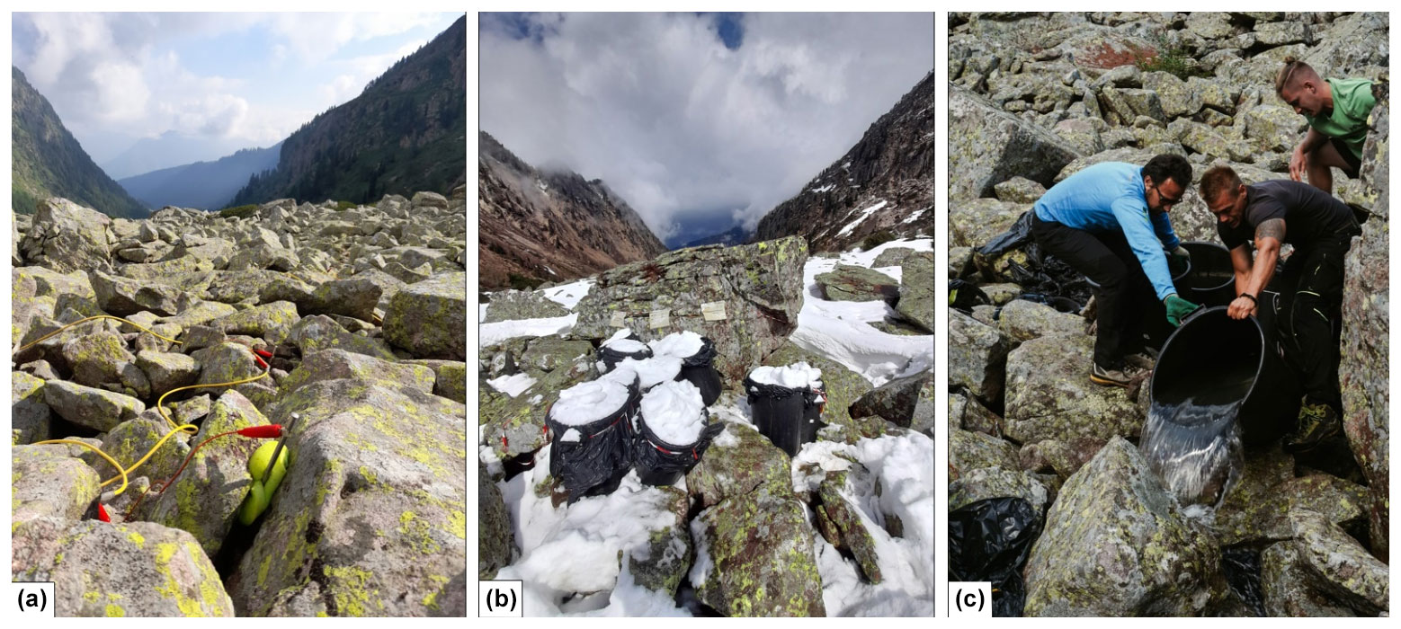
Figure 2 (a) Electrodes inserted between the boulders using sponges soaked with saltwater to improve the contact resistances of the ERT surveys; (b) 10 bins placed at the selected injection point in early spring 2022, filled with snow and covered with nylon sheets pierced at their center to collect rainwater; (c) injection of 800 L of salt water into the subsurface system.

The water for the experiment was collected during the previous months, using ten 100 L bins. The bins were placed on the Sadole rock glacier in the point selected for the water injection, in the early spring when snow cover was still present (Fig. 2b). They were filled with snow and covered with nylon sheets pierced at their center to collect rainwater. This way, in mid-June the bins were completely filled with a mixture of snowmelt and rainwater. Before the experiment, 3 kg of NaCl was added to each bin to obtain a saltwater solution. After collecting the t0 dataset, eight bins were emptied one after the other, injecting 800 L of saltwater into the subsurface system (Fig. 2c). Four datasets were acquired in the first hour, followed by four datasets at hourly intervals, and a last dataset was collected 24 h after water injection. No rain or uncontrolled water contribution happened during the experiment.

3.3 Data processing

The acquired datasets were filtered removing quadrupoles with a stacking error higher than 5 % and a reciprocal error higher than 20 %. Only the common quadrupoles saved in all the filtered datasets were used to perform the inversion process of each dataset. The inversion modeling was performed using the Python-based software ResIPy (Blanchy et al., 2020), and an expected data error of 20 % was defined according to the reciprocal check (Binley, 2015). Once a common unstructured triangular mesh was created, all the acquired datasets were inverted independently. Only the t0 initial model is here plotted in terms of absolute electrical resistivity values (logarithmic scale), while the other models (t_n) obtained with the ERT time-lapse survey are plotted as percentage variations in resistivity compared to the initial model t0. In order to avoid emphasizing changes in the high resistivity zone, the percentage variations in resistivity were calculated using logarithmic values. Since we defined an expected data error of 20 %, tiny resistivity changes in the inverted tomograms are considered not reliable to highlight the flow of the injected water. Therefore, in the time-lapse models, negative resistivity variations lower than 10 % are plotted in light gray color. Finally, to detect the frozen layer boundary in t0 model, we applied the steepest gradient method (Chambers, 2012). This method, as suggested by forward modeling analysis, is the most reliable to evaluate the thickness of the active layer (Herring and Lewkowicz, 2022).

4 Results

Figure 3a shows the t0 resistivity section. The high resistivities (ρ>30 kΩm) close to the surface are linked to the voids among coarse debris and blocks, typical in rock glacier environments (Hauck and Kneisel, 2008). Below this high-resistivity layer, lower values of resistivity (ρ<10 kΩm) are found and can be associated with a decrease in porosity and grain size of the deposit, and a possible increase in humidity. At the southwest and northeast edges of the section, this low-resistivity layer reaches the bottom of the model. On the other hand, in the central part of the model (30<x<70 m) a clear change is detected at a depth of about 10 m. Below this boundary, the resistivity rapidly increases (ρ>50 kΩm), highlighting the presence of a frozen layer (Hauck and Kneisell, 2008). By applying the steepest gradient method in the vertical direction, we defined 55 kΩm as the upper boundary of the permafrost layer, and the same value was used to define its lateral termination.

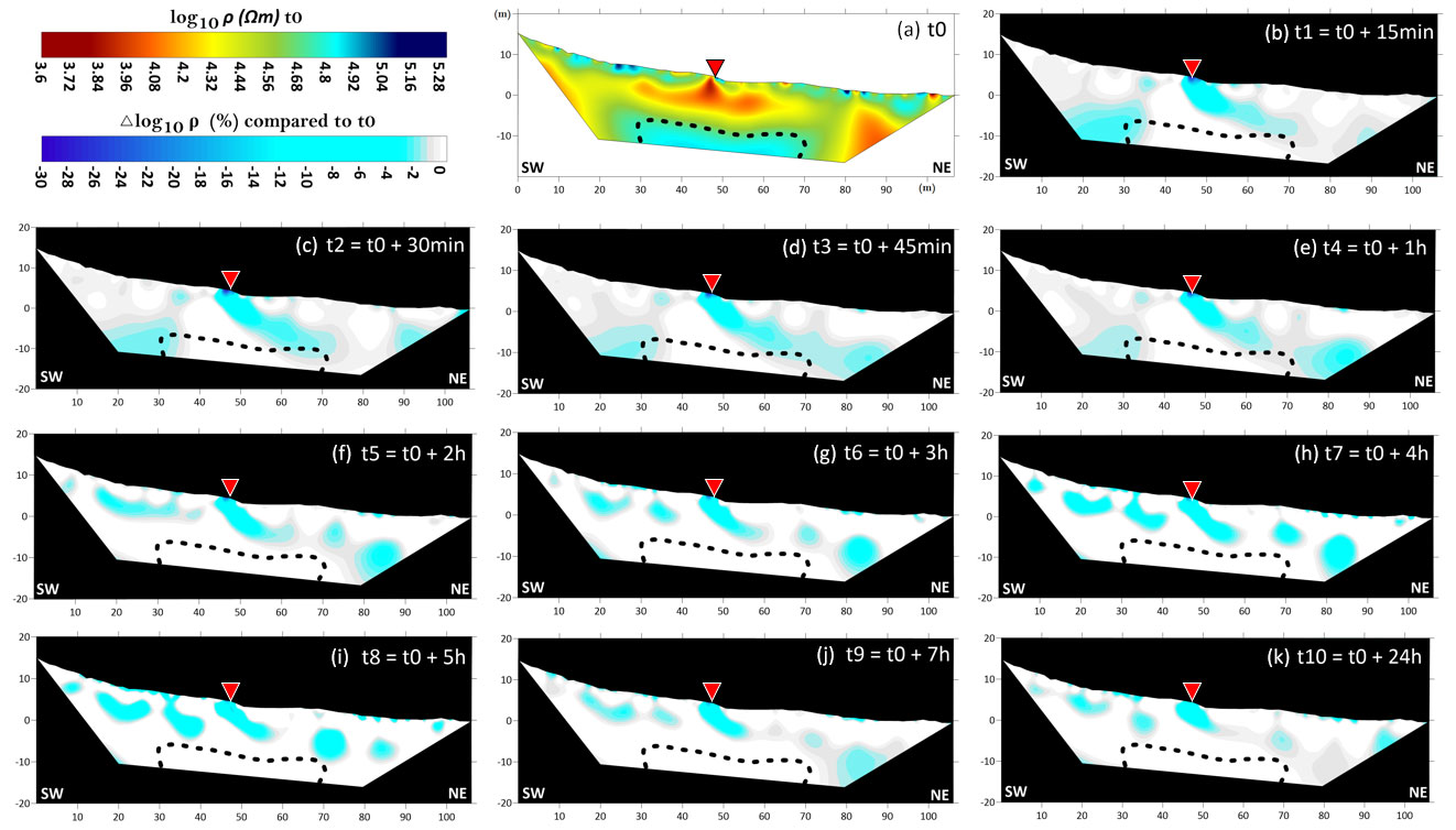
Figure 3 (a) Inverted resistivity section calculated from the t0 dataset. Inverted resistivity variations (%) compared to t0 model, calculated using the logarithmic values, for (b) t1 dataset (t0 + 15 min), (c) t2 dataset (t0 + 30 min), (d) t3 dataset (t0 + 45 min), (e) t4 dataset (t0 + 1 h), (f) t5 dataset (t0 + 2 h), (g) t6 dataset (t0 + 3 h), (h) t7 dataset (t0 + 4 h), (i) t8 dataset (t0 + 5 h), (l) t9 dataset (t0 + 7 h) and (m) t10 dataset (t0 +24 h). The black dashed line represents the boundary of the frozen layer defined applying the steepest gradient method to the inverted resistivity model t0. Red triangles represent the injection point of 800 L of saltwater.

In Fig. 3b high negative resistivity variations (>20 %) show a quick vertical infiltration of the injected water up to a depth of 10 m within the first 15 min after the injection. This wet area persisted below the injection point until the last survey t10 (Fig. 3m), even if it seems to slowly shrink from one data acquisition to the next. Negative resistivity variations in Fig. 3b–e indicate a downslope subsurface flow in the northeast direction above the identified frozen layer. Where the frozen layer ends (x≈70 m), the water clearly appears to be able to propagate deeper vertically. Concerning the upslope area (x<30 m), the negative resistivity variations are found from the surface to the bottom of the section until t4 (Fig. 3b–f), highlighting a main vertical infiltration of the injected water. In the following time steps the negative values develop mainly at few meters of depth (Fig. 3f–l), indicating a possible anomalous upslope subsurface flow (southwest direction). These negative variations, upslope of the injection area, are still present after 24 h (t10, Fig. 3m), but, at the same time, the water still flows downslope in the northeast direction. On the other hand, negative resistivity variations are practically null inside the defined frozen layer, suggesting that the injected water did not propagate through it.

5 Discussion and conclusions

High negative resistivity variations (>20 %) observed for t1 close to the injection area indicate a rapid vertical infiltration of the water due to the presence of boulders, voids, fractures and coarse sediments with high vertical permeability. The large amount of injected water has probably saturated this area, which has become the source of the subsurface flow. Although we do not have any measurements of saturated hydraulic conductivity, we can speculate that hydraulic conductivities may be much higher (on the order of 10⁻² m s⁻¹) than those ones observed in shallow soil layers of young moraines, as found in the Swiss Alps by Maier et al. (2021). Subsurface flow, moving downslope along the northeast direction, likely originated at the boundary between large boulders and a finer sediment. This layer is in fact characterized by lower resistivities (in t0 ρ<10 kΩm) compared to the shallower depths and has likely lower permeability. Nevertheless, the presence of large boulders at various depths can lead to funnel flow and/or splitting of flow paths (Hartmann et al., 2020), which may have determined the infiltration of some injected water upslope (southwest direction) the injection point. From t1 to t5 the negative resistivity variations suggest almost a continuous subsurface flow in the northeast direction along the maximum slope gradient, whereas from t6 to t10 local negative resistivity variations indicate the accumulation of injected water. Most likely these local areas have lower permeability, and water may reside there for a longer period.

The experiment confirms the assumption that a continuous permafrost layer can act as an aquiclude (Giardino et al., 1992; Krainer et al., 2007) or, if it is discontinuous as in the Sadole rock glacier, as an aquitard (Harrington et al., 2018). Furthermore, the survey confirms the reliability of the steepest gradient method to define the boundary of the frozen layer and the high heterogeneities (vertical and lateral) in mountain permafrost subsurface, as recently highlighted from continuous core drilling by Phillips et al. (2023). Due to these high heterogeneities, a quantitative analysis regarding hydraulic conductivity just via time-lapse ERT monitoring is very challenging. As highlighted by Mewes et al. (2017) with synthetic analysis and seasonal field measurements, it is unrealistic to define the flow paths of water in mountain permafrost subsurface just via resistivity changes in tomograms. Moreover, the sampling step of the ERT datasets is forced by their acquisition time and may be too large, especially in the initial phases of the experiment. In our case, due to logistical problems (adverse weather), it was not possible to extend the survey measurements for the time necessary to return completely to the pre-injection conditions.

Future development of the current work is to perform the experiment in an active rock glacier during late summer, in order to test the flow paths with a fully developed active layer, collecting datasets with a shorter sampling step and for a longer period, until the subsurface system returns completely to the pre-injection conditions. In this way, a possible estimation of hydraulic conductivity in the active layer could be achieved.