the Creative Commons Attribution 4.0 License.
the Creative Commons Attribution 4.0 License.
 | 09 Jan 2023
Automated ArcticDEM iceberg detection tool: insights into area and volume distributions, and their potential application to satellite imagery and modelling of glacier–iceberg–ocean systems
Connor J. Shiggins
James M. Lea
Stephen Brough
Iceberg calving accounts for up to half of mass loss from the Greenland Ice Sheet (GrIS), with their size distributions providing insights into glacier calving dynamics and impacting fjord environments through their melting and subsequent freshwater release. Iceberg area and volume data for the GrIS are currently limited to a handful of fjord locations, while existing approaches to iceberg detection are often time-consuming and are not always suited for long time series analysis over large spatial scales. This study presents a highly automated workflow that detects icebergs and appends their associated metadata within Google Earth Engine using high spatial resolution timestamped ArcticDEM (Arctic Digital Elevation Model) strip data. This is applied to three glaciers that exhibit a range of different iceberg concentrations and size distributions: Sermeq Kujalleq (Jakobshavn Isbræ), Umiammakku Isbræ and Kangiata Nunaata Sermia. A total of 39 ArcticDEM scenes are analysed, detecting a total of 163 738 icebergs with execution times of 6 min to 2 h for each glacier depending on the number of DEMs available and total area analysed, comparing well with the mapping of manually digitised outlines. Results reveal two distinct iceberg distributions at Sermeq Kujalleq and Kangiata Nunaata Sermia where iceberg density is high, and one distribution at Umiammakku Isbræ where iceberg density is low. Small icebergs (< 1000 m2) are found to account for over 80 % of each glacier's icebergs; however, they only contribute to 10 %–37 % of total iceberg volume suggesting that large icebergs are proportionally more important for glacier mass loss and as fjord freshwater reservoirs. The overall dataset is used to construct new area-to-volume conversions (with associated uncertainties) that can be applied elsewhere to two-dimensional iceberg outlines derived from optical or synthetic aperture radar imagery. When data are expressed in terms of total iceberg count and volume, insight is provided into iceberg distributions that have potential applicability to observations and modelling of iceberg calving behaviour and fjord freshwater fluxes. Due to the speed and automated nature of our approach, this workflow offers the potential to interrogate iceberg data on a pan-Arctic scale where ArcticDEM strip data coverage allows.
- Article
(6416 KB) - Full-text XML
- BibTeX
- EndNote


Iceberg production is of critical importance when considering the mass balance of ice sheets and glaciers (Bigg et al., 2014), freshwater fluxes (Enderlin et al., 2016; Davison et al., 2020a), offshore infrastructure (Eik and Gudmestad, 2010), shipping, tourism (Bigg, 2015) and ecological habitats (Laidre and Stirling, 2020). Their area–size distributions can be used to infer glacier calving dynamics (Sulak et al., 2017; Scheick et al., 2019; Åström et al., 2021; Cook et al., 2021) and also estimate freshwater fluxes (Enderlin et al., 2016; Moon et al., 2018; Moyer et al., 2019; Davison et al., 2020a). It has been suggested that icebergs could account for up to 22 %–70 % of the total mass loss by 2100 from the Greenland Ice Sheet (GrIS) (Choi et al., 2021), though how future changes in glacier dynamics will influence iceberg size distributions (and vice versa) is currently poorly constrained.
Multiple different approaches have been taken to iceberg detection, including analysis of optical imagery, synthetic aperture radar (SAR) imagery and digital elevation models (DEMs). Semi-automated and/or automated iceberg detection utilising optical imagery typically involves band thresholding to differentiate ice and water (Sulak et al., 2017; Moyer et al., 2019). However, these approaches often use medium-resolution data (10–30 m pixel data, e.g. Landsat and Sentinel-2) that have insufficient spatial resolution to identify the smallest of icebergs or distinguish between larger adjacent icebergs without more complex processing. For example, convolutional neural networks (CNN) have been developed to downsample images, allowing the delineation of smaller iceberg edges at subpixel scale (e.g. Rezvanbehbahani et al., 2020). While CNNs provide opportunities, they are often challenging to construct/validate across large spatial scales and require substantial training data that are obtained from user-intensive manual labelling of images.
In optical imagery, the presence of ice mélange (mixture of icebergs and sea ice) in images also proves problematic for automated band thresholding techniques. This arises due to the similar reflectance signal of mélange to that of icebergs, potentially leading to the generation of erroneously large outlines. Additionally, prolonged cloud cover in some parts of the polar regions and polar night can result in large gaps between observations using optical imagery.
SAR data have the potential for more continuous coverage as the active nature of the sensor can penetrate cloud cover, and do not rely on solar illumination to acquire imagery (e.g. Soldal et al., 2019). However, a notable shortfall of both optical and SAR data is that they are only capable of expressing a surface area of an iceberg, with volumes typically estimated using empirical area–volume relationships derived from DEMs (Sulak et al., 2017; Schild et al., 2021).
Timestamped ArcticDEM version 3 (v3) (Porter et al., 2018) tiles represent an under-exploited resource that allows the derivation of both iceberg areas and their volumes, providing the opportunity to obtain more complete data than optical and/or SAR imagery. These data are obtained from optical stereo-image pairs acquired between 2009 and 2017 and are available in Google Earth Engine (GEE). These pairs provide high spatial resolution DEMs (2 m posting) but have variable temporal coverage due to cloud contamination and satellite image acquisition tasking. While this archive currently has poor return frequency compared with optical and SAR satellite platforms, its spatial resolution and ability to determine iceberg volumes offers the potential for gaining insights that are applicable to the more frequently acquired optical and SAR derived data.
Due to the significant numbers of icebergs existing at any one time in the polar regions, time-intensive manual delineation is not a practical approach to apply to ice-sheet-wide analysis or even at a single glacier site. However, manually digitising icebergs are viable options for (1) creating training sets for supervised classification of semi-automated approaches for a selection of image scenes (Sulak et al., 2017) and (2) generating highly targeted datasets of icebergs, e.g. the Canadian ice island drift, deterioration and detection (CI2D3) database (Crawford et al., 2018).
Iceberg area distributions have previously been used to constrain glacier calving dynamics (Scheick et al., 2019) and determine iceberg disintegration processes (Kirkham et al., 2017). These distributions have previously been described using power laws in particle modelling studies (Åström et al., 2021) and from imagery in areas adjacent to glacier termini, to gain insight into calving dynamics in both Greenland (Enderlin et al., 2016; Sulak et al., 2017; Scheick et al., 2019; Rezvanbehbahani et al., 2020) and Antarctica (Tournadre et al., 2016; England et al., 2020). These relationships describe probability distributions of iceberg size, with Eq. (1) describing the general form of these relationships,
where p(x) is the distribution with x representing either area (A) or volume (V), C is a constant and α is the exponent of the power law (or slope value). The value of α (reported hereafter including the negative sign in Eq. 1) provides an indication of iceberg size distributions at the time of data acquisition with lower values suggesting a higher prevalence of smaller icebergs, whereas more positive values indicate that relatively larger icebergs dominate. Typical α values for Greenlandic and Antarctic environments have been reported between −1.2 and −3.0. As icebergs drift from Greenland's termini to the open ocean, their distributions have been observed to transition from being best described as power law distributions (suggested to be controlled by calving) to lognormal distributions as melting becomes the primary control on their disintegration (Kirkham et al., 2017).
When fitting icebergs to power law distributions and calculating α, it is important to determine a threshold which removes icebergs below a certain area–size (xmin). Where smaller icebergs are included in the distribution, these can result in less robust fits with power laws because they follow different size distributions compared with larger icebergs (Kirkham et al., 2017). Including smaller icebergs in this analysis can therefore skew the α value and potentially misrepresent the data (as discussed in Scheick et al., 2019). Given the larger surface area to volume ratios of smaller icebergs, it is also more likely that their different size distribution arises from more extensive modification by submarine and atmospherically driven melting. Defining the appropriate xmin value is therefore critical for investigations that seek to determine how iceberg size is impacted by glacier calving processes.
A further complexity of the xmin value is that if the value is defined too high, there will be significant data loss that will limit the explanatory value of the distribution. This is especially the case for glaciers where there is a high proportion of small icebergs. An example of where it has previously been appropriate to set a high xmin value is at Sermeq Kujalleq (Jakobshavn Isbræ), where Scheick et al. (2019) defined an xmin of 1800 m2 as they were primarily interested in larger icebergs that occur more frequently at this glacier, and the xmin set improved the fit compared with other values tested. In other studies, the resolution of imagery available has impacted the range of xmin values that can be defined. For example, CNN performed on planet imagery (3 m optical imagery) resulted in xmin values of 288 and 387 m2, while Sentinel-2 (10 m optical imagery) required values of 12 000 and 3200 m2 for Sermilik and Kangerlussuaq Fjords, respectively (Rezvanbehbahani et al., 2020). This demonstrates how the availability of finer spatial resolution data can in some cases also allow the definition of smaller xmin values and the retention of more data.
Few studies (e.g. Sulak et al., 2017) have been able to directly estimate iceberg volume, as optical and/or SAR imagery are (without significant further processing) limited to the extraction of iceberg areas only. The three-dimensional shape of an iceberg above the waterline allows its volume to be inferred, though it does not always scale exactly with its planform area. For example, rafts of icebergs frozen together by mélange/fjord ice that occur at some glaciers will be relatively flatter and have a lower volume compared with single icebergs of the same area that have calved from a glacier. Applying a single iceberg area to volume conversion determined from iceberg data to these rafts would therefore lead to an over-estimation of their volumes.
One of the current difficulties faced by those studying the impact of icebergs on fjords is the lack of available iceberg outline and volume data that are suitable for use in numerical models of fjord circulation, stratification and iceberg melting (e.g. Moon et al., 2018; Davison et al., 2020a). Models that include the quantification of iceberg meltwater flux currently assume iceberg area–volume distributions within fjords, though direct observations of these from satellite data are rarely available (e.g. Davison et al., 2020a). This issue is compounded by the time and computational expense involved in the detection of icebergs (e.g. data collection, storage, memory and processing). One solution to this is offered by the GEE cloud computing platform (Gorelick et al., 2017) which provides the ability to rapidly access and process data from multiple different satellites, offering the potential for ice-sheet-wide and global analysis (e.g. Shugar et al., 2020).
This study provides a GEE workflow and easy-to-use graphical user interface (GUI), using 2 m strip ArcticDEM v3 data (Porter et al., 2018) to automatically detect icebergs at three marine-terminating glaciers on the west coast of Greenland. The aim of this study is to demonstrate the ability of the workflow to automatically generate a large and reliable dataset of icebergs from glaciers of varying size and fjord conditions. In doing so the workflow aims to allow users to gain detailed insight into iceberg area–volume relationships and identify how these vary between glaciers.
Three different marine-terminating glaciers were selected to conduct analysis, identified on the basis of their different fjord environments, iceberg sizes and data availability: (1) dense large iceberg coverage: Sermeq Kujalleq (Jakobshavn Isbræ) (hereafter SKJI); (2) a mix of dense iceberg coverage and frequent open water: Umiammakku Isbræ (hereafter UI); and (3) dense small iceberg coverage with occasional open water: Kangiata Nunaata Sermia (hereafter KNS) (Fig. 1). Regions of interest (ROI) at each glacier were identified to maximise ArcticDEM data availability and reduce the impact of winter/spring seasonal advance of the caving margin during the study period of 2009–2017.
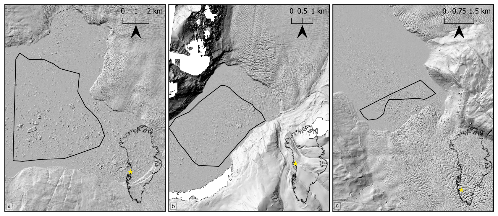
Figure 1ArcticDEM imagery of the near terminus region for (a) Sermeq Kujalleq: 69.16∘ N, 49.91∘ W, (b) Umiammakku Isbræ: 71.42∘ N, 52.26∘ W and (c) Kangiata Nunaata Sermia: 64.25∘ N, 49.50∘ W. The ROIs for each glacier are mapped by black bounding boxes.
SKJI accounts for 45 % of the total drainage of Greenland's central west sector, with a mean ice discharge (2010–2018) of 43.64 Gt yr−1 (Fig. 1a) (Mankoff et al., 2020; Mouginot et al., 2019). Ice mélange buttressing of its terminus can inhibit calving, influence flow and allow advance (e.g. Amundson et al., 2010; Cassotto et al., 2021). Between 2011 and 2017, SKJI experienced a range of grounding line depths varying from 828 to 980 m (Morlighem et al., 2017; Khazendar et al., 2019), producing icebergs as large as 700–1000 m across, forcing ice mélange down-fjord because of full-thickness calving events (Amundson et al., 2010; Walter et al., 2012). The retreat of SKJI from an annually floating terminus which calved larger icebergs (2000–2002) has led to a seasonally grounded terminus, causing much smaller icebergs to be calved during the summer months (2013–2015) (Scheick et al., 2019).
UI has a mean ice discharge (2010–2018) of 1.36 Gt yr−1 (see Fig. 1b) (Mankoff et al., 2020), with terminus depths ranging from 230 to 500 m between 2013 and 2015 (Carroll et al., 2016; Morlighem et al., 2017; Fried et al., 2018). Prior to the study period between 2003 and 2008, UI experienced a substantial (4 km) rapid retreat of its terminus (Bartholomaus et al., 2016; Fahrner et al., 2021).
KNS is the largest marine-terminating glacier south of SKJI on the west coast of Greenland with a mean ice discharge (2010–2018) of 4.92 Gt yr−1 (see Fig. 1c) (Mankoff et al., 2020). It has retreated over 23 km from its Little Ice Age maximum position (Lea et al., 2014a, b) but has remained relatively stable in the past decade (Davison et al., 2020b; Fahrner et al., 2021). The glacier's fjord is typically filled with mélange of small icebergs and brash ice and currently has a relatively shallow grounding line depth of approximately 250 m (Morlighem et al., 2017). While the development of a channelised, subglacial hydrological system at KNS increases localised calving activity due to greater submarine melt and plume surfacing, it decreases terminus-wide calving and suggests that high levels of runoff could decrease the number of calving events (Bunce et al., 2021).
3.1 ArcticDEM data
The availability of ArcticDEM within GEE and its high 2 m spatial resolution (10 cm vertical accuracy) is used to create a highly automated workflow to delineate icebergs and derive their individual volumes, which are validated against manually digitised outlines. The workflow is also packaged in a GUI with a respective GitHub page that contains the necessary information on how to access the tool, define an ROI and export the data to a user's Google Drive or GEE asset (see: https://github.com/ConnorShiggins/Google-Earth-Engine-and-icebergs, last access: 3 January 2023). To ensure a consistent level of high-quality data, analysis is automatically limited to only include DEMs generated from stereopair images acquired on the same day. In doing so, this limits the effect of iceberg drift, ensuring that only the highest-quality DEMs are analysed. DEMs acquired between the months of July and October are analysed to avoid the presence of seasonal floating ice tongues that form and persist through winter and spring that could lead to erroneous results. The data availability for each glacier is variable, with KNS having 16 available images from 4 July 2013 to 26 August 2017, SKJI 20 images ranging from 8 July 2011 to 9 August 2017 and UI 3 images between 4 July 2012 and 3 July 2017.
3.2 Workflow description
The only user defined input required for the code to execute is an ROI (Fig. 2); the users can also modify other parameters (see below). The workflow dynamically filters the ArcticDEM image collection to retain DEMs with > 80 % coverage of the ROI, before scenes with low image quality (e.g. cloud affected) are removed by calculating the 90th percentile of a scene's elevation and ensuring that it is within ±10 m of the WGS84 geoid.
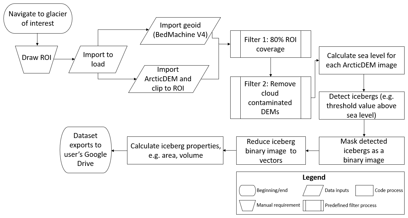
To allow for potentially poor spatial registration in the Z dimension of the DEM and different tidal states at the time of data acquisition, sea level is automatically calculated for each individual DEM. This is achieved by assuming that when DEM elevation values over the fjord are plotted as a histogram with 0.25 m bin widths, its peak (i.e. the most common elevation in the DEM) represents sea level at the time the image was acquired (Appendix A, Fig. A1). This allows each DEM to be registered to a common base level (i.e. 0 m above sea level) for consistent iceberg identification, and calculation of iceberg freeboard height and volume. The results in this study are limited to analysing DEMs acquired between July and October to minimise the likelihood of rigid mélange and sea ice being present at the ice front, though users are able to define any time period of interest. If a DEM contains these conditions and bypasses the pre-defined filters, it will return an erroneously high sea level for each iceberg (appended as metadata), meaning that these DEMs can be easily identified and potentially removed from the resulting dataset during post-processing.
To delineate iceberg outlines, it is necessary to separately define a threshold value above sea level where icebergs can be confidently delineated without multiple icebergs being erroneously merged. Consequently, derived iceberg areas and volumes from the workflow represent minimum estimates. Potential threshold values for each glacier were explored using increments of 0.1 m between 0.1 and 1.5 m for KNS and UI (glaciers where small icebergs dominate), whereas this was increased to 0.5 m increments between 1.0 and 5.0 m for SKJI where dense concentrations of large icebergs exist. There are extremely small variations (∼ 0.04) in the power law slopes at SKJI, providing reason for testing the detection threshold increments by 0.5 m. From these results, the most appropriate iceberg detection threshold was evaluated through visual comparison with manually digitised iceberg outlines. From this, the most appropriate threshold was determined to be 1.5 m above sea level for KNS and UI, and 3.0 m for SKJI. The workflow uses the threshold value to identify any area above sea level where it is exceeded as an iceberg. Depending on the type of fjord environment (e.g. densely packed, open water) and the research question being addressed, the user can potentially alter the default iceberg detection threshold of 1.5 m above sea level within the workflow (see GitHub read.me).
Within the workflow, areas of the DEM that exceed the threshold are converted to a binary image (1 = iceberg, 0 = no iceberg) which is then vectorised into iceberg outlines. Iceberg-specific metadata (e.g. area, volume) are appended to each outline automatically, using DEM input data where needed. The final part of the workflow removes any large object (> 100 000 m2) in case of false iceberg detection by erroneously delineating fjord edges and/or the glacier termini before the user can either choose to export results to the Google Drive in their preferred file format (e.g. CSV, Shapefile or GeoJSON) or to a GEE asset.
3.3 Iceberg distributions
Once exported from the GUI, iceberg areas and volumes from each glacier are fitted to power law distributions as described in Eq. (1) using the “powerlaw” package in Python (Alstott et al., 2014). To allow consistent comparison of how power law distributions evolve through time, xmin values are kept the same for every image, defined as 500 m2 for KNS and UI, and 1000 m2 for SKJI. The lower xmin value of 500 m2 for KNS and UI was chosen as they produce smaller icebergs compared with SKJI, meaning that 1000 m2 value would have resulted in significant data loss. Both values assigned for the three glaciers allowed reduced skewing of the α exponent and provided more robust fits to power law distributions. The xmin values defined are also within the range used by previous studies and provided internal consistency for each glacier dataset (e.g. Sulak et al., 2017; Scheick et al., 2019; Rezvanbehbahani et al., 2020). The ability to determine iceberg area and volume for each iceberg in the dataset allowed the derivation of an empirical area-to-volume conversion expressed as a power law relationship following Sulak et al. (2017).
4.1 Workflow evaluation
The ROI at SKJI was 41 and 9.6 km2 at UI and 5.3 km2 at KNS with the number of detected icebergs across all available images ranging from 6973 at UI to 147 714 at SKJI (Table 1). For each individual glacier, iceberg distributions obtained from automated and manual delineation methods were found to be qualitatively and quantitatively comparable (Pearson's r value = 0.70–0.96) (Figs. 3 and 4; Table 1).
Table 1Data from the three glaciers, including the ROI size, the date of the ArcticDEM image which was manually validated, number of images in the entire collection, number of icebergs detected, both automated and manual power law slope values (with one sigma) for area with corresponding xmin (total iceberg volume below and above the respective value: SKJI = 1000 m2; UI and KNS = 500 m2) and the execution time. The error attached to the automated power law slope is one standard deviation derived in the “powerlaw” Python package.

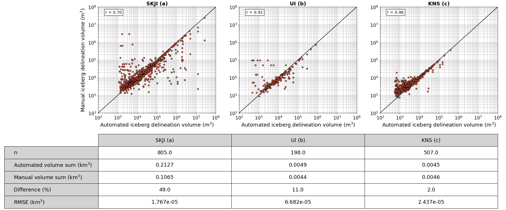
Figure 3The relationship between the iceberg volume for both the manual and automated delineation methods for each glacier and respective summary statistics. Each point in subplots (a), (b) and (c) represent a specific iceberg that has been mapped by both the automated and manual delineations. Iceberg volume derivations for both delineation methods were performed in GEE with the associated ArcticDEM as input data, assuming that the icebergs were neutrally buoyant. Pearson's correlation coefficient is also highlighted (SKJI = 0.70, UI = 0.92, KNS = 0.96).
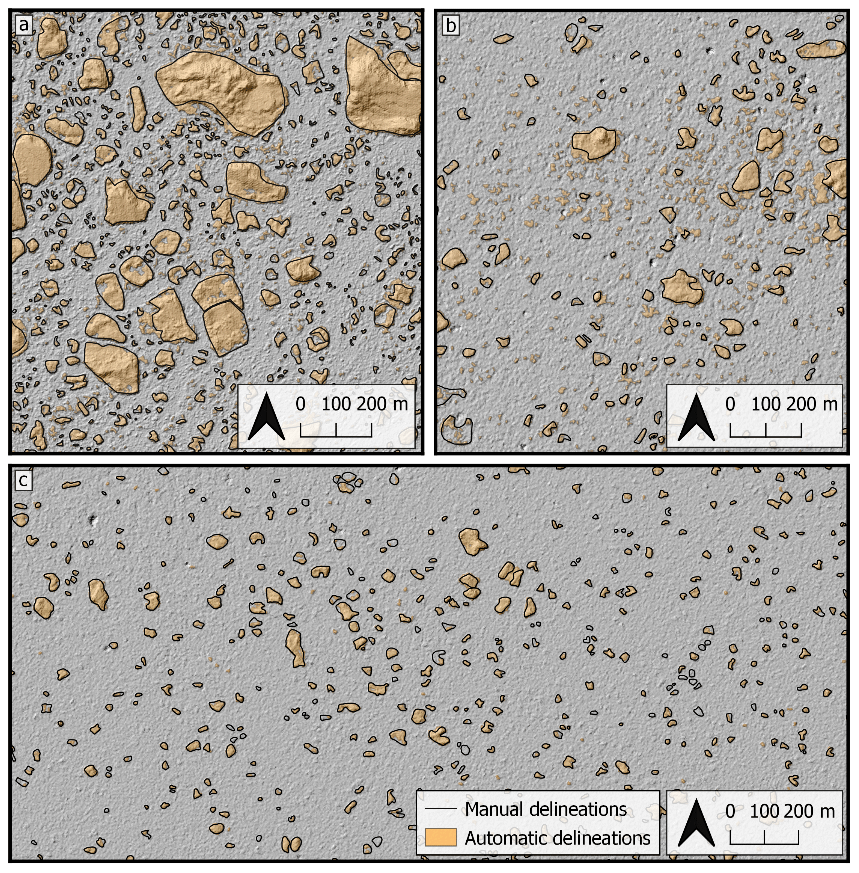
Figure 4Manual (black lines) and automated (orange) delineations of the iceberg subset for (a) SKJI (10 September 2011), (b) UI (4 July 2012) and (c) KNS (21 August 2013) overlaying the hillshaded ArcticDEM v3 strip data for each glacier.
For each ArcticDEM scene throughout the study period at each glacier, sea level ranged from 23 to 39 m, broadly following the local geoid sea level elevation. Visual comparison between manual and automatically delineated data for each threshold showed that threshold values of 1.5 m above sea level for KNS and UI, and 3.0 m above sea level for SKJI (Fig. 5), provided the best visual correspondence and provided more concordant power law fits with manually digitised outlines (Fig. 6; see Data and Methods).

Figure 5Iceberg frequency for each threshold value tested. (a) SKJI's values were performed for 0.5 m increments between 0 and 5 m above sea level. Increments of 0.1 m between 0 and 1.5 m above sea level were run for both (b) UI and (c) KNS. Panel (d) shows how the α value for each glacier changes depending on which threshold value is chosen to detect its respective iceberg. Note the log scale on the y axis in the subplot: (a)–(c).
Iceberg area–size distributions of both the manually and automated methods are found to follow power law distributions for the xmin values applied (Fig. 6). Results reveal that SKJI has the least negative power law slope (1.88) of the three glaciers followed by UI (2.16) and KNS has the most negative values (2.38), correctly highlighting that icebergs at SKJI are generally larger than those at UI or KNS (Fig. 4). Good correspondence between automatically and manually delineated iceberg area α values were observed for SKJI and UI where they differed by 0.03 and 0.01 for SKJI and UI respectively, though this increased to 0.39 at KNS. Power law relationships applied to iceberg volume distributions for each of the glaciers showed similar results; however, the difference in the α value reduces to 0.02, 0.01 and 0.20 at SKJI, UI and KNS respectively.
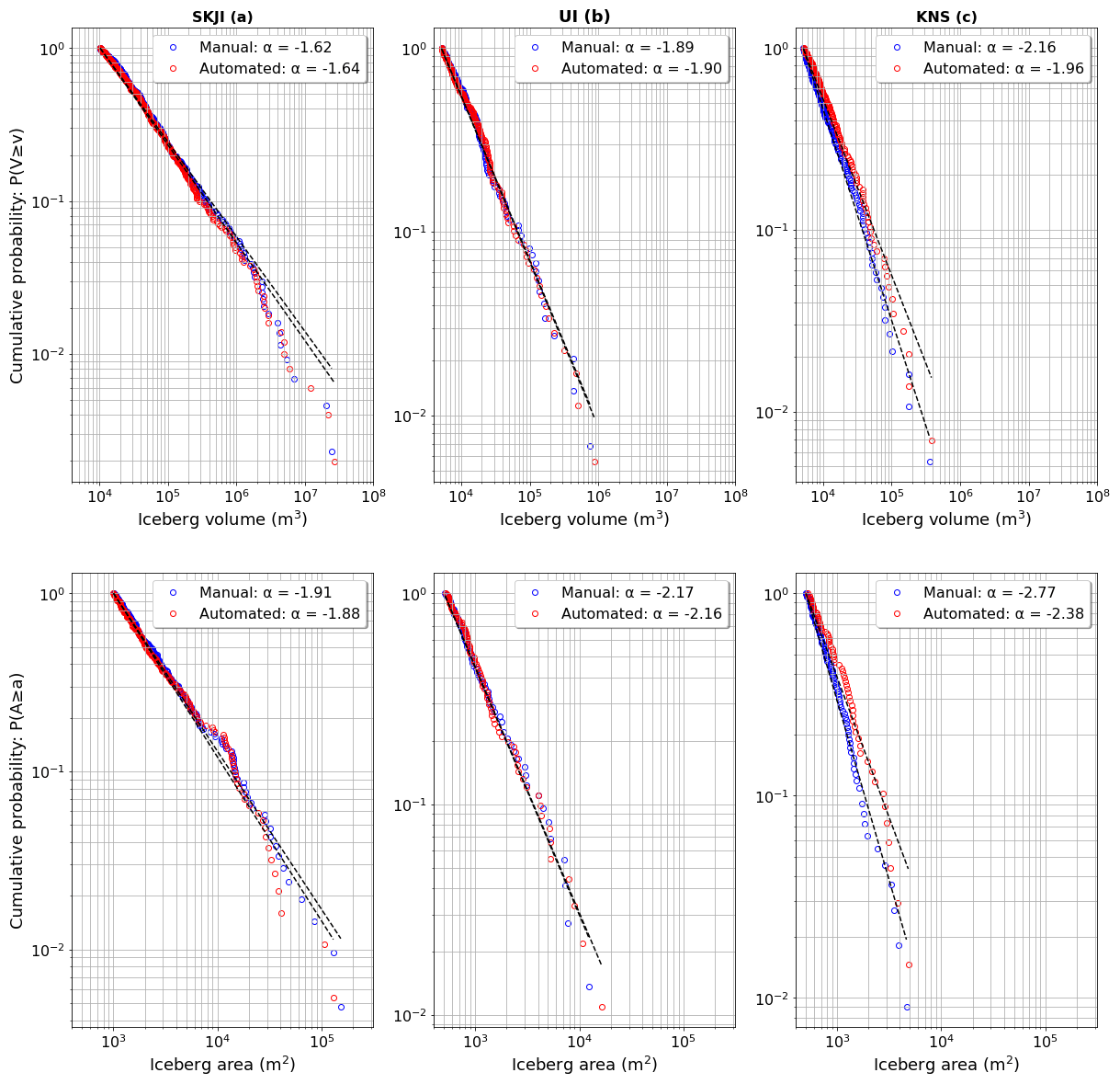
Figure 6Power law plots for the manual (blue open circles) and automatically (red open circles) delineated icebergs. For iceberg area: (a) SKJI has an xmin value defined at 1000 m2, compared with 500 m2 for both (b) UI and (c) KNS. For defining an xmin for iceberg volume distributions, the respective area xmin value was converted using the equation of Sulak et al. (2017; their Eq. 5) yielding a value of 10 270 m3 for SJKI and 5135 m3 for UI and KNS. The black lines show the line of best fit for the iceberg distributions. Note that the y axis is plotting cumulative probability where alpha equals −1.
4.2 Iceberg area and volume distributions
The three-dimensional nature of DEMs allows the volume of each iceberg to be calculated assuming neutral buoyancy (ice density = 920 kg m−3, seawater density = 1025 kg m−3), allowing the derivation of the relationship between planform iceberg area (A) and volume (V) (Fig. 7). To reduce the potential for biasing power law relationships towards more frequently observed smaller icebergs, the relationships reported are derived from binned means using bin increments of log10(A+0.1). For the entire iceberg dataset this can be expressed as
The large nature of the dataset also allows equations describing the lower and upper confidence bounds to be derived, with the 5th percentile of the distribution described by
and the 95th percentile of the distribution described by
When compared with the previously published area-to-volume conversion equation of Sulak et al. (2017; their Eq. 5), their relationship would produce lower volumes for small area icebergs (area = < 1000 m2; Rezvanbehbahani et al., 2020) and higher volumes for large area icebergs (Fig. 7).
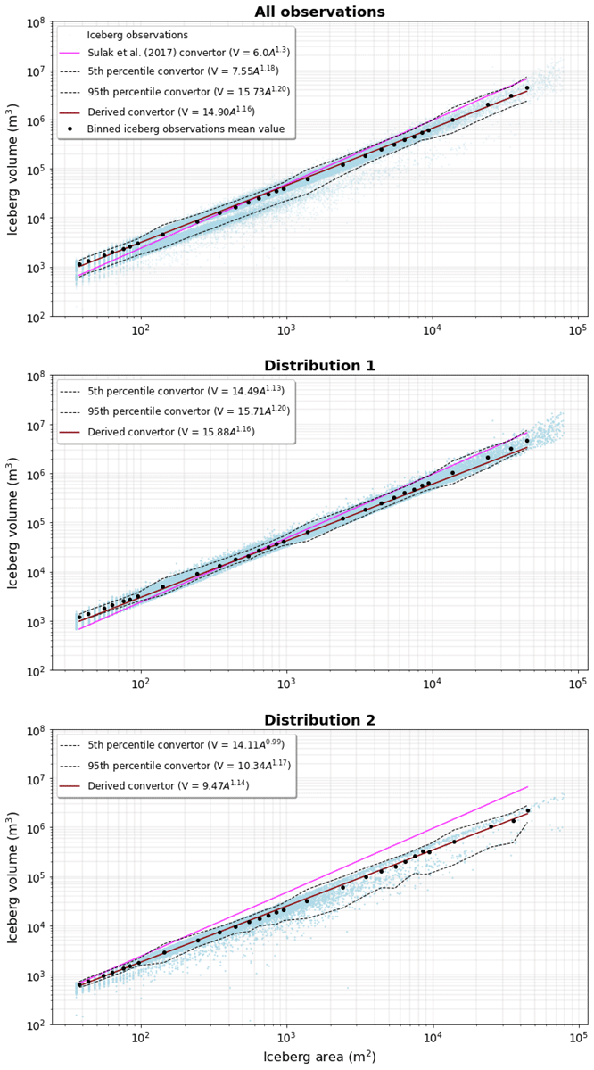
Figure 7The mean iceberg area and volume for each size class (e.g. mean of 30–40 m2, mean of 100–200 m2, mean of 1000–2000 m2 and so on) for each glacier, overlaid with the Sulak et al. (2017) conversion (pink) and the one derived here (brown). By calculating mean iceberg area and volume within log10(A+0.1) binned increments, this reduced the potential for biasing area–volume relationships towards smaller, more frequently observed icebergs. The top plot contains all the icebergs in the dataset for each glacier, while the middle and lower plots contain the icebergs residing in distribution 1 and distribution 2, respectively. Uncertainty in these distributions is also characterised by deriving similar relationships for the 5 % and 95 % limits. To note, these limits are derived from the binned mean size classes and are therefore not straight.
When observing how iceberg area scales with volume, two distinct distributions are identified at SKJI and KNS (Fig. 8; Table 2), persisting between individual DEMs throughout the study period. Visual inspection of hillshaded DEMs indicates that distribution 1 is characterised by single iceberg outlines, while distribution 2 comprises some single icebergs and iceberg rafts. Combining data from SKJI and KNS, distribution 2 accounts for only 7.2 % of the icebergs in the population, with its divergence from distribution 1 found to proportionately increase with iceberg area (Fig. 8 insets). Each of the two distributions can be expressed using power law relationships in a similar manner to the overall distribution, with the equations for distribution 1 (red) and distribution 2 (blue) shown in Eqs. (5) and (6) respectively (Fig. 7b, c):
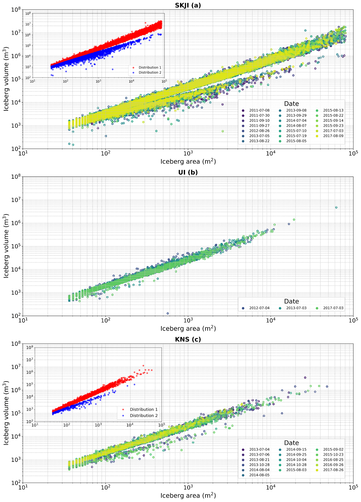
Figure 8Iceberg area versus volume which is colour coded by each ArcticDEM scene date. The inset in both the SKJI (a) and KNS (c) panels shows the two distributional branches identified in the data. Each distribution is separated by identifying local minima in probability distribution histograms of the entire dataset.
Table 2Summary statistics of the two distributions outlined at SKI and KNS.

a distribution 1; b distribution 2. SD: standard deviation.
In the entire dataset, small icebergs (area = < 1000 m2; Rezvanbehbahani et al., 2020) account for over 80 % of the total iceberg count for each glacier; however, they only contribute to 10 %, 37 % and 35 % of the total volume at SKJI, UI and KNS, respectively (Fig. 9). Consequently, while small icebergs dominate the distributions in the fjord of each glacier, compared with larger icebergs they are found to account for a significantly smaller proportion of total iceberg volume.
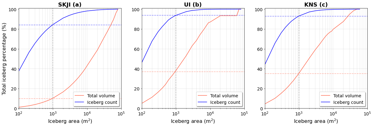
Figure 9Cumulative iceberg volume (orange line) and count (blue line) plotted as percentage with their respective surface area. The small iceberg threshold (< 1000 m2) is defined by a dashed grey line. The total volume made up by small icebergs is represented by the dashed orange line and the total number is the dashed blue line.
5.1 Workflow
The workflow presented here allows users to successfully delineate icebergs and capture their area and volume size distributions and assign a range of metadata to each individual iceberg (Fig. 6). The workflow therefore allows users to rapidly obtain iceberg data to interrogate glacier calving styles and iceberg freshwater fluxes. The application of the workflow to glacier fjords with a range of different iceberg concentrations and sizes demonstrates the utility of ArcticDEM data for iceberg detection and mapping across a range of different fjord environments typical of Greenland and elsewhere. As a result, this approach is suitable for pan-Arctic iceberg detection where availability of DEM data allow (see Appendix A, Fig. A2).
This new method is quick to execute and is capable of successfully filtering ArcticDEM scenes by cloud contamination, ROI data coverage and dynamically defining sea level for each ArcticDEM scene to account for potentially poor image registration and local tidal state. While this results in the rejection of scenes with data gaps and partial cloud contamination where parts of the image may be suitable for analysis, the automated image filtering steps implemented in the workflow removes the requirement for time-consuming user-led data cleaning. These filters (e.g. ROI coverage) can also be manually adjusted by the user if required (see GitHub read.me).
The detection thresholds defined (1.5 m for KNS and UI and 3.0 m for SKJI) are found to be suitable for correctly delineating iceberg outlines and subsequent size distributions (Fig. 4). Though a mismatch in size distributions is found at KNS where small icebergs dominate, it is likely that this arises from operator bias in the manual delineation of these icebergs. This arises due to the manual operator delineating icebergs across pixels in the DEM compared with the automated approach that only identifies icebergs through whole pixel analysis. In this instance, the workflow therefore provides a more complete footprint of small icebergs than a manual digitiser is able. Visual comparison of iceberg outlines produced by the workflow to multi-angle hillshaded DEMs (Fig. 4) provides confidence that it is able to detect icebergs as small as 40 m2 (10 pixels). However, larger proportionate mismatches in area are expected between manual and automated delineation methods for smaller icebergs, explaining the mismatch in power law slope values observed at KNS (Fig. 6).
Exploration of the workflow's sensitivity to increasing the detection threshold above sea level shows that higher thresholds detect only larger icebergs and will result in fractionally smaller overall iceberg areas and volumes of these larger icebergs (Fig. 5). The user definition of this detection threshold is dependent on whether smaller icebergs are important to include for the user's research question. Where only the largest icebergs are of interest, a higher detection threshold could therefore be set with relatively little loss in the final iceberg areas and volumes. This is because volumetrically larger icebergs are more likely to have higher freeboard heights, and the iceberg margins omitted due to higher thresholds are likely to be small in terms of their relative area and volume. We show that by defining different xmin, values between SKJI (1000 m2) and UI and KNS (500 m2) can result in the retention of a significant proportion of iceberg data (Fig. 9). As highlighted by previous studies (e.g. Sulak et al., 2017; Scheick et al., 2019; Rezvanbehbahani et al., 2020) and shown here, the definition of xmin is therefore critical for ensuring sufficient data are available for analysis.
As a consequence, those wishing to explore power law size distribution relationships where small icebergs are less important for a user's research question can potentially set a higher detection threshold. Conversely, if a study is wanting to retain the maximum number of icebergs for subsequent analysis, a lower threshold could be defined, though this risks outlines of neighbouring icebergs being erroneously identified as a single iceberg. This is highlighted by the fact that rafts of small individual icebergs frozen together by mélange are correctly identified by the workflow as single floating bodies of ice, though the individual icebergs that they are composed of are not separated out by the workflow. If a user's research question requires both iceberg and iceberg raft cover (distributions 1 and 2) within an ROI, the default threshold of 1.5 m above sea level is suitable, as is the 3.0 m threshold for more densely ice-covered fjords such as SKJI. If only iceberg outlines are needed, a higher detection could be defined to remove iceberg rafts (distribution 2). It is noteworthy that setting a higher detection threshold would result in the potential loss of data relating to smaller icebergs which have lower freeboard heights and fractionally lower iceberg volumes obtained from larger icebergs. An alternative approach that would retain smaller icebergs and not result in the minor under-estimation of iceberg volume would be to use a lower threshold (e.g. 1.5 or 3 m), with data from distributions 1 and 2 separated as part of post-processing (e.g. Fig. 8 insets). While it is emphasised that all results from the workflow are likely to represent minimum area and volume estimates, it is suggested that for the majority of cases a threshold of 1.5 m should be sufficient.
Choosing different ROIs at the same glacier can result in varying numbers of DEMs available for analysis because of the workflow filters (Fig. 2) and spatial coverage of ArcticDEM v3 strip data. This is more pronounced at glaciers with wider termini (e.g. SKJI), rather than narrower fjords, as data are more likely to cover the terminus (e.g. KNS). For example, by subsetting three ROIs at SKJI, it is apparent that the number of available DEMs varies from 4 to 30 across the ice front and provides different power law slope values (−1.78 to −2.03) (Fig. 10). Whether these differences in power law slopes are solely dependent on the amount of data available is not currently possible to ascertain, as these may also be a product of variable calving dynamics across the ice front (i.e. different calving styles between northern, central and southern ice front sections at SKJI).

Figure 10Subset sampling across SKJI's ice front to determine how iceberg distributions change spatially. Overlaying the hillshaded ArcticDEM image are the total iceberg collections for each subset with the respective power law slopes beneath, corresponding by both letter and colour. The “n” underneath each iceberg collection is the number of available DEMs within the subsetted ROI.
5.2 Glaciological implications
The new area-to-volume conversions presented offer the potential for wide-scale application to iceberg area outline data that have been derived from optical and/or SAR imagery (Eqs. 2–6; Fig. 7). The large dataset generated also allows for the quantification of uncertainties when scaling area-to-volume (Eqs. 3 and 4 for 5th and 95th percentiles respectively; Fig. 7). This will allow iceberg volumes to be estimated from data sources that extend beyond the spatial and temporal availability of ArcticDEM and that are more frequently acquired (e.g. Landsat satellites and Sentinel-1 and -2). Improved constraint of uncertainties in iceberg volumes therefore provide new opportunities for temporally and spatially extending studies that seek to model fjord freshwater fluxes (Davison et al., 2020a) and quantify iceberg volume distributions (e.g. Schild et al., 2021). While it should be remembered that the conversion equations result in minimum volume estimates, inclusion of lower and upper limits will assist in better quantification of ranges of potential iceberg volume from iceberg outline data alone.
We find evidence of two iceberg populations at SKJI and KNS across multiple ArcticDEM scenes between 2010 and 2017, though only a single population at UI (Fig. 8). The DEM surface expression of icebergs identified in the second distribution tend to be flatter than those of distribution 1, resulting in lower overall volumes. Manual inspection of DEMs suggests that the majority of those in distribution 2 represent rafts of small icebergs that are frozen together by mélange. Though distribution 1 dominates the total dataset, studies using two-dimensional data (i.e. optical and/or SAR) should be aware that their methods may identify these iceberg rafts as single icebergs. For glaciers where these two iceberg distributions exist, using a single area-to-volume conversion will therefore result in an overestimation of total iceberg volume. It may therefore be appropriate for users to separate out these distributions during post-processing and apply Eqs. (5) and (6) to obtain complete volume estimates (e.g. Fig. 7). To identify iceberg rafts from two-dimensional image data it may be required to undertake further analysis (e.g. approaches that go beyond pixel level analysis; for example, incorporating iceberg level image texture as part of machine learning methods, e.g. Rezvanbehbahani et al., 2020).
The two distributions noted at SKJI and KNS suggest that different populations are present in fjords across Greenland, representing icebergs and ice rafts respectively. The evolution of both populations through time is currently challenging as ArcticDEM v3 data at the study sites occur irregularly through seasons and between years. This means that identification of seasonal and multi-annual timescale changes in these distributions cannot currently be characterised with confidence. However, with the recent (October 2022) release of more temporally comprehensive ArcticDEM v4 strip data we anticipate that it will become possible to use the workflow for detailed time series analysis on sub-annual to multi-annual timescales. At the time of writing, these data are yet to be ingested into GEE; however, if and when they are, the workflow will be updated to be made available within the GUI.
Results show that small icebergs (area = < 1000 m2) account for the majority of those identified (over 80 % for each glacier) yet contribute a smaller fraction of the total iceberg volume (10 %–37 % of total volume; Fig. 9). Consequently, small differences in the number of large icebergs can have a disproportionate impact on overall fjord iceberg volume. At these glaciers, large icebergs therefore represent comparatively larger freshwater reservoirs in their fjords and account for a more significant proportion of overall ice mass loss from their source glaciers.
Expressing iceberg counts and volumes for each glacier as percentages (Fig. 9) also offers the potential for empirically estimating the evolution of iceberg populations for individual ice sheet outlets from frequently updated velocity derived glacier discharge data (e.g. Mankoff et al., 2020). Although this would assume a consistent calving style through time, such relationships could assist in estimating how the number and volumes of icebergs have evolved; may evolve in the future (through application to ice discharges from ice dynamic modelling, e.g. Choi et al., 2021); and assessment of potential iceberg hazards.
This study presents a new workflow and GUI to automatically detect icebergs within Google Earth Engine using ArcticDEM, offering the potential to significantly and rapidly expand iceberg area and volume datasets. Results from the workflow show good agreement with manually digitised iceberg outlines (r values = 0.70, 0.92, 0.96), with mismatches occurring for the smallest of icebergs where the precision of manual digitisation is poorer compared with that of the workflow. The workflow identifies two distinct iceberg populations at SKJI and KNS and one at UI representing (1) individual icebergs and (2) small iceberg rafts frozen together by mélange. The significantly greater amount of data generated by the workflow has allowed derivation of new area-to-volume conversion equations for each distribution including upper and lower bound uncertainties for the first time. While smaller icebergs at each glacier are found to dominate the distributions (84 %–94 % of the total count), their contribution to total volume and therefore freshwater flux are relatively small (10 %–37 %).
Although ArcticDEM data are temporally and spatially limited relative to those obtained by optical and SAR satellite platforms, the results presented here offer the potential for extending studies into fjord iceberg cover and glacier calving that use iceberg outlines derived from these data. A new approach of expressing relationships between iceberg count and volume will also allow empirical estimation of iceberg size distributions from iceberg discharge observations. This would have benefits to those investigating iceberg freshwater fluxes within fjords and who seek to model the evolution of mass loss from the GrIS.
The workflow and user interface presented here allow users to generate their own large, reliable datasets for their glacier(s) of interest. Consequently, it opens the possibility of extending the results presented here to any location where suitable ArcticDEM data are available.
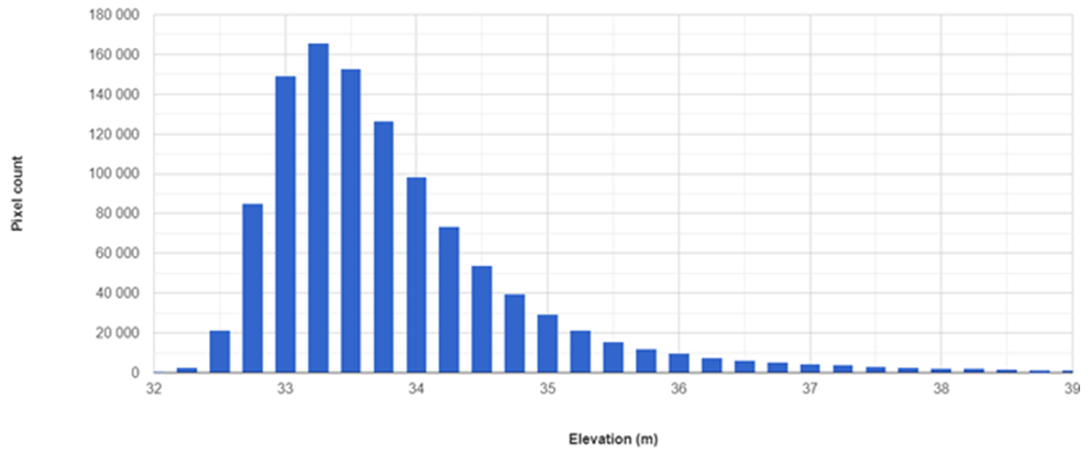
Figure A1Example of an automated histogram calculated within GEE of elevation pixel count in an ArcticDEM image at KNS (4 July 2013). The elevation with the highest pixel count is automatically selected as the sea level for that scene. In this example sea level would be 33.25 m.
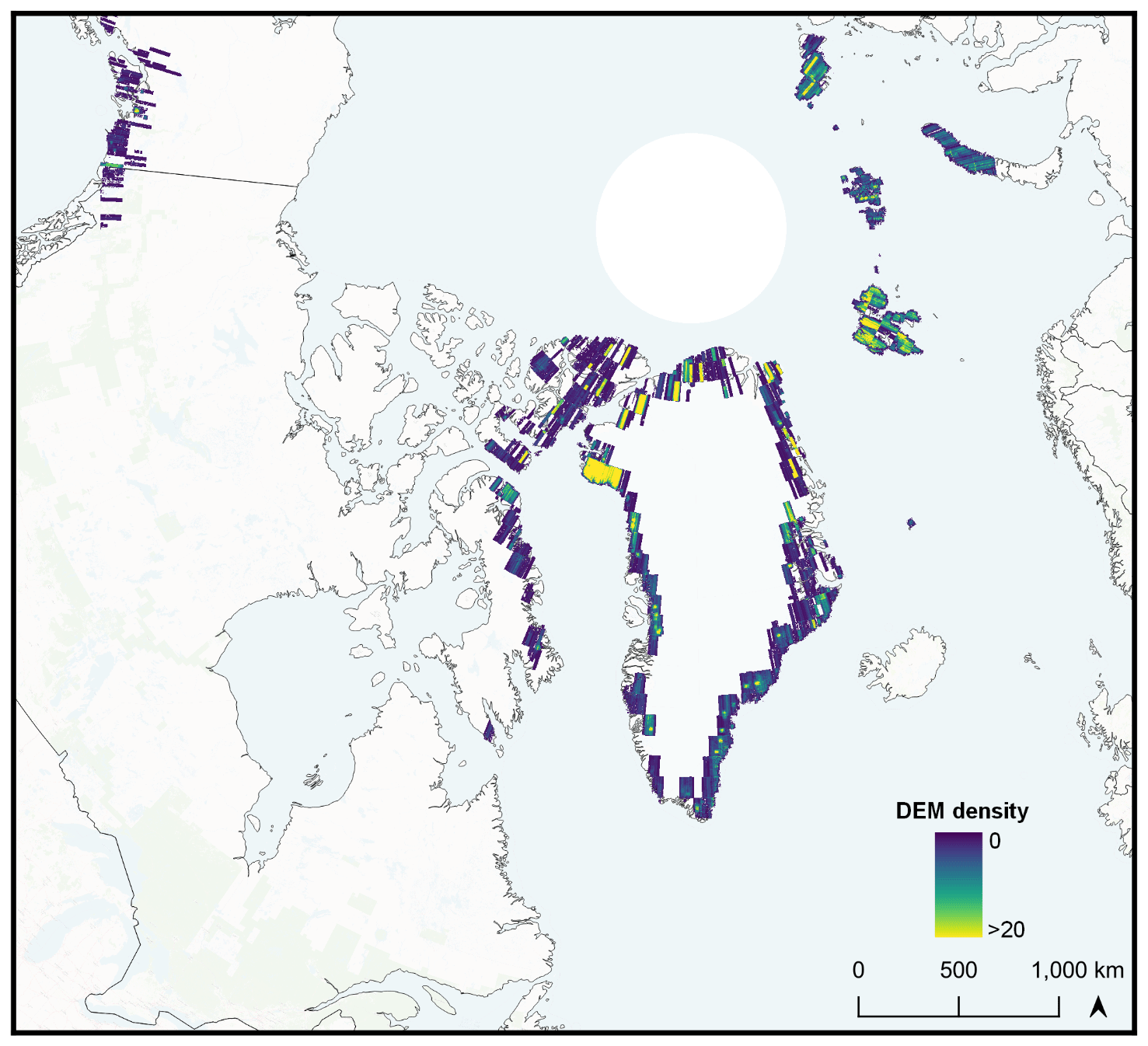
Figure A2© Google Earth Engine ArcticDEM v3 strip data availability (July–October) for Greenland's calving margins and all marine/lake/shelf terminating glaciers' extent in the remainder of the Arctic.
The user-interface guide to generate an iceberg dataset is available on the GitHub site (https://github.com/ConnorShiggins/Google-Earth-Engine-and-icebergs, last access: 3 January 2023) and Zenodo (https://doi.org/10.5281/zenodo.7500735, Shiggins, 2023) and a direct link to the tool can be accessed through the Google Earth Engine Code Editor (https://code.earthengine.google.com/ec7218374595f2a3053c72a2d6b4211d, Shiggins, 2023).
The workflow to generate the iceberg dataset is available using Google Earth Engine which is a free to use cloud computing platform for individual licenses. The metadata for all the iceberg data can be found alongside the source code on a Zenodo repository: https://doi.org/10.5281/zenodo.7500735 (Shiggins, 2023).
CJS and JML conceived the study. CJS produced the dataset, conducted all the analyses and led the manuscript writing. JML and SB offered conceptual and coding advice, and contributed to the writing of the manuscript.
The contact author has declared that none of the authors has any competing interests.
Publisher's note: Copernicus Publications remains neutral with regard to jurisdictional claims in published maps and institutional affiliations.
We thank Dominik Fahrner for providing terminus positions for Umiammakku Isbræ. We are grateful to the Polar Geospatial Center for the development and accessibility of ArcticDEM. The authors thank the editor Pippa Whitehouse, Till Wagner and an anonymous reviewer for their insightful comments.
Connor J. Shiggins, PhD studentship, is funded by the University of Liverpool. James M. Lea is supported by a UKRI Future Leaders Fellowship (grant No. MR/S017232/1).
This paper was edited by Pippa Whitehouse and reviewed by Till Wagner and one anonymous referee.
Alstott, J., Bullmore, E., and Plenz, D.: powerlaw: a Python package for analysis of heavy-tailed distributions, PloS one, 9, e85777, https://doi.org/10.1371/journal.pone.0095816, 2014.
Amundson, J. M., Fahnestock, M., Truffer, M., Brown, J., Lüthi, M. P., and Motyka, R. J.: Ice mélange dynamics and implications for terminus stability, Jakobshavn Isbræ, Greenland, J. Geophys. Res.-Earth, 115, F01005, https://doi.org/10.1029/2009JF001405, 2010.
Åström, J., Cook, S., Enderlin, E. M., Sutherland, D. A., Mazur, A., and Glasser, N.: Fragmentation theory reveals processes controlling iceberg size distributions, J. Glaciol., 67, 1–10, https://doi.org/10.1017/jog.2021.14, 2021.
Bartholomaus, T. C., Stearns, L. A., Sutherland, D. A., Shroyer, E. L., Nash, J. D., Walker, R. T., Catania, G., Felikson, D., Carroll, D., Fried, M. J., and Noël, B. P.: Contrasts in the response of adjacent fjords and glaciers to ice-sheet surface melt in West Greenland, Ann. Glaciol., 57, 25–38, https://doi.org/10.1017/aog.2016.19, 2016.
Bigg, G. R.: Icebergs: their science and links to global change, Cambridge University Press, https://doi.org/10.1017/CBO978110758927, 2015.
Bigg, G. R., Wei, H. L., Wilton, D. J., Zhao, Y., Billings, S. A., Hanna, E., and Kadirkamanathan, V.: A century of variation in the dependence of Greenland iceberg calving on ice sheet surface mass balance and regional climate change, Proc. R. Soc. A, 470, 20130662, https://doi.org/10.1098/rspa.2013.0662, 2014.
Bunce, C., Nienow, P., Sole, A., Cowton, T., and Davison, B.: Influence of glacier runoff and near-terminus subglacial hydrology on frontal ablation at a large Greenlandic tidewater glacier, J. Glaciol., 67, 343–352, https://doi.org/10.1017/jog.2020.109, 2021.
Carroll, D., Sutherland, D. A., Hudson, B., Moon, T., Catania, G. A., Shroyer, E. L., Nash, J. D., Bartholomaus, T. C., Felikson, D., Stearns, L. A., and Noel, B. P.: The impact of glacier geometry on meltwater plume structure and submarine melt in Greenland fjords, Geophys. Res. Lett, 43, 9739–9748, https://doi.org/10.1002/2016GL070170, 2016.
Cassotto, R. K., Burton, J. C., Amundson, J. M., Fahnestock, M. A., and Truffer, M.: Granular decoherence precedes ice mélange failure and glacier calving at Jakobshavn Isbræ, Nat. Geosci., 14, 417–422, https://doi.org/10.1038/s41561-021-00754-9, 2021.
Choi, Y., Morlighem, M., Rignot, E., and Wood, M.: Ice dynamics will remain a primary driver of Greenland ice sheet mass loss over the next century, Commun. Earth Environ., 2, 1–9, https://doi.org/10.1038/s43247-021-00092-z, 2021.
Cook, S. J., Christoffersen, P., Truffer, M., Chudley, T. R., and Abellan, A.: Calving of a large Greenlandic tidewater glacier has complex links to meltwater plumes and mélange, Geophys. Res.-Earth, 126, e2020JF006051, https://doi.org/10.1029/2020JF006051, 2021.
Crawford, A., Crocker, G., Mueller, D., Desjardins, L., Saper, R., and Carrieres, T.: The Canadian ice island drift, deterioration and detection (CI2D3) database, J. Glaciol., 64, 517–521, https://doi.org/10.1017/jog.2018.36, 2018.
Davison, B. J., Cowton, T. R., Cottier, F. R., and Sole, A. J.: Iceberg melting substantially modifies oceanic heat flux towards a major Greenlandic tidewater glacier, Nat. Commun., 11, 1–13, https://doi.org/10.1038/s41467-020-19805-7, 2020a.
Davison, B. J., Sole, A. J., Cowton, T. R., Lea, J. M., Slater, D. A., Fahrner, D., and Nienow, P. W.: Subglacial drainage evolution modulates seasonal ice flow variability of three tidewater glaciers in southwest Greenland, J. Geophys. Res.-Earth, 125, e2019JF005492, https://doi.org/10.1029/2019JF005492, 2020b.
Eik, K. and Gudmestad, O. T.: Iceberg management and impact on design of offshore structures, Cold Reg. Sci. Technol., 63, 15–28, https://doi.org/10.1016/j.coldregions.2010.04.008, 2010.
Enderlin, E. M., Hamilton, G. S., Straneo, F., and Sutherland, D. A.: Iceberg meltwater fluxes dominate the freshwater budget in Greenland's iceberg-congested glacial fjords, Geophys. Res. Lett., 43, 11–287, https://doi.org/10.1002/2016GL070718, 2016.
England, M. R., Wagner, T. J. W., and Eisenman, I.: Modeling the breakup of tabular icebergs, Sci. Adv., 6, eabd1273, https://doi.org/10.1126/sciadv.abd1273, 2020.
Fahrner, D., Lea, J. M., Brough, S., Mair, D. W., and Abermann, J.: Linear response of the Greenland ice sheet's tidewater glacier terminus positions to climate, J. Glaciol., 67, 193–203, https://doi.org/10.1017/jog.2021.13, 2021.
Fried, M. J., Catania, G. A., Stearns, L. A., Sutherland, D. A., Bartholomaus, T. C., Shroyer, E., and Nash, J.: Reconciling drivers of seasonal terminus advance and retreat at 13 Central West Greenland tidewater glaciers, J. Geophys. Res.-Earth, 123, 1590–1607, https://doi.org/10.1029/2018JF004628, 2018.
Gorelick, N., Hancher, M., Dixon, M., Ilyushchenko, S., Thau, D., and Moore, R.: Google Earth Engine: Planetary-scale geospatial analysis for everyone, Remote Sens. Environ., 202, 18–27, https://doi.org/10.1016/j.rse.2017.06.031, 2017.
Khazendar, A., Fenty, I. G., Carroll, D., Gardner, A., Lee, C. M., Fukumori, I., Wang, O., Zhang, H., Seroussi, H., Moller, D., and Noël, B. P:. Interruption of two decades of Jakobshavn Isbrae acceleration and thinning as regional ocean cools, Nat. Geosci., 12, 277–283, https://doi.org/10.1038/s41561-019-0329-3, 2019.
Kirkham, J. D., Rosser, N. J., Wainwright, J., Jones, E. C. V., Dunning, S. A., Lane, V. S., Hawthorn, D. E., Strzelecki, M. C., and Szczuciński, W.: Drift-dependent changes in iceberg size-frequency distributions, Sci. Rep., 7, 1–10, https://doi.org/10.1038/s41598-017-14863-2, 2017.
Laidre, K. L. and Stirling, I.: Grounded icebergs as maternity denning habitat for polar bears (Ursus maritimus) in North and Northeast Greenland, Polar Biol., 43, 937–943, https://doi.org/10.1007/s00300-020-02695-2, 2020.
Lea, J. M., Mair, D. W., Nick, F. M., Rea, B. R., Weidick, A., Kjaer, K. H., Morlighem, M., Van As, D., and Schofield, J. E.: Terminus-driven retreat of a major southwest Greenland tidewater glacier during the early 19th century: insights from glacier reconstructions and numerical modelling, J. Glaciol., 60, 333–344, https://doi.org/10.3189/2014JoG13J163, 2014a.
Lea, J. M., Mair, D. W. F., Nick, F. M., Rea, B. R., van As, D., Morlighem, M., Nienow, P. W., and Weidick, A.: Fluctuations of a Greenlandic tidewater glacier driven by changes in atmospheric forcing: observations and modelling of Kangiata Nunaata Sermia, 1859–present, The Cryosphere, 8, 2031–2045, https://doi.org/10.5194/tc-8-2031-2014, 2014b.
Mankoff, K. D., Solgaard, A., Colgan, W., Ahlstrøm, A. P., Khan, S. A., and Fausto, R. S.: Greenland Ice Sheet solid ice discharge from 1986 through March 2020, Earth Syst. Sci. Data, 12, 1367–1383, https://doi.org/10.5194/essd-12-1367-2020, 2020.
Moon, T., Sutherland, D. A., Carroll, D., Felikson, D., Kehrl, L., and Straneo, F.: Subsurface iceberg melt key to Greenland fjord freshwater budget, Nat. Geosci., 11, 49–54, https://doi.org/10.1038/s41561-017-0018-z, 2018.
Morlighem, M., Williams, C. N., Rignot, E., An, L., Arndt, J. E., Bamber, J. L., Catania, G., Chauché, N., Dowdeswell, J. A., Dorschel, B., Fenty, I., Hogan, K., Howat, I., Hubbard, A., Jakobsson, M., Jordan, T. M., Kjeldsen, K. K., Millan, R., Mayer, L., Mouginot, J., Noël, B., O'Cofaigh, C., Palmer, S. J., Rysgaard, S., Seroussi, H., Siegert, M. J., Slabon, P., Straneo, F., van den Broeke, M. R., Weinrebe, W., Wood, M., and Zinglersen, K.: BedMachine v3: Complete bed topography and ocean bathymetry mapping of Greenland from multi-beam echo sounding combined with mass conservation, Geophys. Res. Lett., 44, 11051–11061, https://doi.org/10.1002/2017GL074954, 2017.
Mouginot, J., Rignot, E., Bjørk, A. A., Van den Broeke, M., Millan, R., Morlighem, M., Noël, B., Scheuchl, B., and Wood, M.: Forty-six years of Greenland Ice Sheet mass balance from 1972 to 2018, P. Natl. Acad. Sci. USA, 116, 9239–9244, https://doi.org/10.1073/pnas.1904242116, 2019.
Moyer, A. N., Sutherland, D. A., Nienow, P. W., and Sole, A. J.: Seasonal variations in iceberg freshwater flux in Sermilik Fjord, southeast Greenland from Sentinel-2 imagery, Geophys. Res. Lett., 46, 8903–8912, https://doi.org/10.1029/2019GL082309, 2019.
Porter, C., Morin, P., Howat, I., Noh, M.-J., Bates, B., Peterman, K., Keesey, S., Schlenk, M., Gardiner, J., Tomko, K., Willis, M., Kelleher, C., Cloutier, M., Husby, E., Foga, S., Nakamura, H., Platson, M., Wethington Jr., M., Williamson, C., Bauer, G., Enos, J., Arnold, G., Kramer, W., Becker, P., Doshi, A., D'Souza, C., Cummens, P., Laurier, F., and Bojesen, M.: ArcticDEM, Version 3, Harvard Dataverse V1 [data set], https://doi.org/10.7910/DVN/OHHUKH, 2018.
Rezvanbehbahani, S., Stearns, L. A., Keramati, R., Shankar, S., and van der Veen, C. J.: Significant contribution of small icebergs to the freshwater budget in Greenland fjords, Commun. Earth Environ, 1, 1–7, https://doi.org/10.1038/s43247-020-00032-3, 2020.
Scheick, J., Enderlin, E. M., and Hamilton, G.: Semi-automated open water iceberg detection from Landsat applied to Disko Bay, West Greenland, J. Glaciol., 65, 468–480, https://doi.org/10.1017/jog.2019.23, 2019.
Schild, K. M., Sutherland, D. A., Elosegui, P., and Duncan, D.: Measurements of iceberg melt rates using high-resolution GPS and iceberg surface scans, Geophys. Res. Lett., 48, e2020GL089765, https://doi.org/10.1029/2020GL089765, 2021.
Shiggins, C.: ConnorShiggins/Google-Earth-Engine-and-icebergs: V2_icebergs (V2_icebergs), Zenodo [code], https://doi.org/10.5281/zenodo.7500735, 2023.
Shugar, D. H., Burr, A., Haritashya, U. K., Kargel, J. S., Watson, C. S., Kennedy, M. C., Bevington, A. R., Betts, R. A., Harrison, S., and Strattman, K.: Rapid worldwide growth of glacial lakes since 1990, Nat. Clim. Change, 10, 939–945, https://doi.org/10.1038/s41558-020-0855-4, 2020.
Soldal, I. H., Dierking, W., Korosov, A., and Marino, A.: Automatic detection of small icebergs in fast ice using satellite wide-swath SAR images, Remote Sens., 11, 806, https://doi.org/10.3390/rs11070806, 2019.
Sulak, D. J., Sutherland, D. A., Enderlin, E. M., Stearns, L. A., and Hamilton, G. S.: Iceberg properties and distributions in three Greenlandic fjords using satellite imagery, Ann. Glaciol., 58, 92–106, https://doi.org/10.1017/aog.2017.5, 2017.
Tournadre, J., Bouhier, N., Girard-Ardhuin, F., and Rémy, F.: Antarctic icebergs distributions 1992–2014, J. Geophys. Res.-Oceans, 121, 327–349, https://doi.org/10.1002/2015JC011178, 2016.
Walter, F., Amundson, J. M., O'Neel, S., Truffer, M., Fahnestock, M., and Fricker, H. A.: Analysis of low-frequency seismic signals generated during a multiple-iceberg calving event at Jakobshavn Isbræ, Greenland, J. Geophys. Res.-Earth, 117, F01036, https://doi.org/10.1029/2011JF002132, 2012.