Linking scales of sea ice surface topography: evaluation of ICESat-2 measurements with coincident helicopter laser scanning during MOSAiC

Information about sea ice surface topography and related deformation is crucial for studies of sea ice mass balance, sea ice modeling, and ship navigation through the ice pack. The Ice, Cloud, and land Elevation Satellite-2 (ICESat-2), part of the National Aeronautics and Space Administration (NASA) Earth Observing System, has been on orbit for over 4 years, sensing the sea ice surface topography with six laser beams capable of capturing individual features such as pressure ridges. To assess the capabilities and uncertainties of ICESat-2 products, coincident high-resolution measurements of sea ice surface topography are required. During the yearlong Multidisciplinary drifting Observatory for the Study of Arctic Climate (MOSAiC) expedition in the Arctic Ocean, we successfully carried out a coincident underflight of ICESat-2 with a helicopter-based airborne laser scanner (ALS), achieving an overlap of more than 100 km. Despite the comparably short data set, the high-resolution centimeter-scale measurements of the ALS can be used to evaluate the performance of ICESat-2 products. Our goal is to investigate how the sea ice surface roughness and topography are represented in different ICESat-2 products as well as how sensitive ICESat-2 products are to leads and small cracks in the ice cover. Here, we compare the ALS measurements with ICESat-2's primary sea ice height product, ATL07, and the high-fidelity surface elevation product developed by the University of Maryland (UMD). By applying a ridge-detection algorithm, we find that 16 % (4 %) of the number of obstacles in the ALS data set are found using the strong (weak) center beam in ATL07. Significantly higher detection rates of 42 % (30 %) are achieved when using the UMD product. While only one lead is indicated in ATL07 for the underflight, the ALS reveals many small, narrow, and only partly open cracks that appear to be overlooked by ATL07.

1 Introduction

Sea ice is not a planar surface but rather appears in a wide range of multifaceted shapes. While level ice is the product of solely thermodynamic ice growth, mechanical processes produce deformed ice. In the presence of wind and waves, ice floes can collide with each other and pile up into pressure ridges. These ridges can appear as almost linear features in the sea ice surface topography. The height of sea ice ridges above the surrounding level ice, known as the sail height, is required for the estimation of drag coefficients. These drag coefficients indicate the intensity of air–ice interactions in the momentum balance equation describing the ice motion in sea ice models (Tsamados et al., 2014; Castellani et al., 2014; Mchedlishvili et al., 2023). The geometry of ridges also plays a role in the distribution of snow on sea ice. Snow is redistributed continuously via wind and accumulates at obstacles such as pressure ridges (Wagner et al., 2022). Eventually, the deformation of sea ice becomes an important factor for the sea ice mass balance and thickness distribution (Ricker et al., 2021; von Albedyll et al., 2022).

On the other hand, in the case of divergent forces, the ice cover breaks apart leaving open water in the form of cracks and leads. The width of these openings can vary from a few meters to more than a kilometer. Leads are important for energy transfer between the ocean and atmosphere as well as for the optimal routing of vessels through the ice-covered ocean. Detecting and measuring the dimensions of sea ice surface features like ridges and leads is therefore essential to improve our understanding of the Arctic climate system.

Information on sea ice surface features is also important for deriving the sea ice freeboard – the height of the ice surface above the water level – from satellite altimetry. Specifically, the detection of leads is required for calculating the sea ice freeboard (Ricker et al., 2014). Moreover, for the interpretation of radar altimetry measurements over sea ice, roughness plays a major role. Landy et al. (2020) showed that variable sea ice surface roughness contributes a systematic uncertainty to the sea ice freeboard and thickness retrievals from the European Space Agency CryoSat-2 satellite.

Information and precise mapping of sea ice surface topography exist mostly from direct measurements acquired during field campaigns, ship-based surveys, or ice camps. However, retrieving continuous basin-scale information about the evolution and distribution of deformed ice, ridges, and leads is difficult. Satellite altimeters like CryoSat-2 are capable of detecting leads and measuring the freeboard (Wingham et al., 2006; Quartly et al., 2019), but they cannot resolve the surface topography to the level that is required to measure the dimensions of ridges, such as the sail height (Johnson et al., 2022). However, the development of satellite altimeter sensors is advancing, and the National Aeronautics and Space Administration (NASA) launched the Ice, Cloud, and land Elevation Satellite-2 (ICESat-2) in 2018. ICESat-2 carries the photon-counting Advanced Topographic Laser Altimeter System (ATLAS), which surveys the ground with six beams, arranged in three pairs, and each beam has a nominal footprint diameter of around 11 m (Magruder et al., 2020). The instrument's small footprint size and high pulse repetition rate allow for unprecedented measurements of sea ice surface topography. Kwok et al. (2019a) demonstrated that ICESat-2 is capable of resolving rough surface topography via comparisons with airborne laser altimetry measurements. Fredensborg Hansen et al. (2021) used the geolocated photon heights from ICESat-2 to estimate the degree of sea ice ridging in the Bay of Bothnia. Recently, Farrell et al. (2020) developed a high-fidelity product that optimizes the use of information retrieved by the photon-counting technique to detect individual ridges, leads, and melt ponds, and a recent study by Duncan and Farrell (2022) showed the distribution of pressure ridges at the basin scale. So far, these ICESat-2 surface elevation products have been mostly benchmarked against airborne lidar measurements from Operation IceBridge (OIB). Kwok et al. (2019a) used lidar data from a campaign in spring 2019 operating at an altitude of ∼ 1000 m, resulting in footprints of ∼ 2 m, which were sufficient to verify the presence of ridges and leads; however, to capture the exact dimensions of ridges and surface features, validation data of an even higher resolution are required. Moreover, if we want to understand how the photon heights relate to the surface roughness within the illuminated area of the footprints, we need detailed and accurate measurements of the surface topography within the illuminated areas of the beams.

Here, we present a new validation data set for ICESat-2 sea ice measurements that was acquired during the Multidisciplinary drifting Observatory for the Study of Arctic Climate (MOSAiC) campaign (Nicolaus et al., 2022). The helicopter aboard the drifting research vessel (RV) Polarstern was equipped with an airborne laser scanner (ALS) capable of sensing the sea ice surface with a lateral resolution of a few centimeters (Jutila et al., 2022b). ALS surveys were carried out during the entire MOSAiC drift, providing a unique data set of sea ice surface topography through a full seasonal cycle. On 23 March 2020, we followed an ICESat-2 ground track in close vicinity for 130 km, achieving an overlap between the ALS swath and the center beam pair of about 90 %. Although this was the only coincident helicopter flight, we will show that, even with a short data set, a comprehensive verification of the ICESat-2 sea ice surface elevation products is possible. Other helicopter ALS surveys have not been used in this study, as a direct comparison between surface features appearing in the airborne and satellite data is difficult or not possible otherwise. This study will link the MOSAiC ALS measurements with ICESat-2 measurements in order to investigate the evolution of the surface topography and deformation of the sea ice near the MOSAiC camp in the context of regional and Arctic-wide changes captured by ICESat-2. We pursue the following goals. First, we aim to validate the ICESat-2 ATL07 (Sea Ice Heights, Level 3A) product (Kwok et al., 2021a), which contains along-track heights for sea ice relative to the WGS84 ellipsoid as well as parameters useful for the detection of open-water leads, such as the return and background photon rates. For comparison, we will use the high-resolution ALS surface elevations as well as the ALS reflectance, which is used to detect leads. Second, we seek to investigate how the surface roughness within the ATL07 segments/footprint is related to the height estimates. Third, we aim to quantify the degree to which the true dimensions of sea ice surface topography, given by the ALS, can be captured by ICESat-2 products. Therefore, we will use the official NASA release of the ATL07 product as well as the high-fidelity Ridge Detection Algorithm (RDA) product provided by the University of Maryland (Farrell et al., 2020; Duncan and Farrell, 2022), denoted UMD-RDA hereafter. Finally, we will compare the weak and strong beams with respect to the objectives mentioned above.

Another aim of this study is to demonstrate that the increasing resolution of satellite altimeters will require that validation strategies be adapted. In fact, being able to relate individual surface features to altimeter signals allows for smaller, more flexible, and less extensive campaigns, in addition to the large-scale campaigns that cover different ice regimes and regions. Mapping the dimensions of sea ice surface topography requires validation with high-resolution sensors, in contrast with the validation of previous altimeters (e.g., CryoSat-2) that was primarily based on comparing large-scale averages.

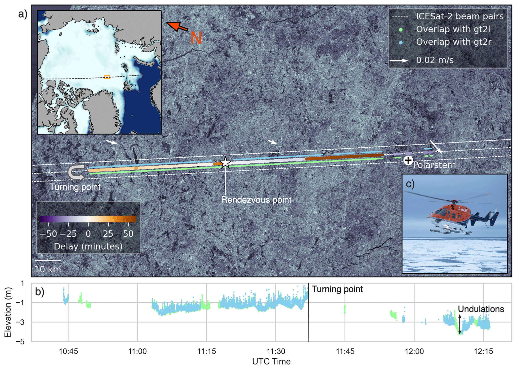
Figure 1 (a) Overview of helicopter flight and airborne laser scanner measurements (ALS) coinciding with the Ice, Cloud, and land Elevation Satellite-2 (ICESat-2) center beam pair, comprising the weak (gt2l) and strong (gt2r) beam. The upper left box shows the location of the zoomed-in position as an orange rectangle. The time delay of ALS data acquisition is shown for the overlapping sections. Note that part of the overlap was achieved on the return flight to RV Polarstern. The position of RV Polarstern corresponds to the time of helicopter takeoff. The background shows a Sentinel-1 radar image on the day of the flight, obtained from FRAM-Sat (2020) in the framework of the MOSAiC project. White arrows show the low-resolution sea ice drift from the Ocean and Sea Ice Satellite Application Facility (OSI SAF). (b) Elevations of the overlapping ALS measurements along the helicopter flight track before the correction of undulations, relative to the Technical University of Denmark mean sea surface (DTU21 MSS). Note that the gt2l elevation profile is partly masked by gt2r. Also note that, on the return section after the turning point, only those sections are shown where overlap was not achieved on the outbound flight. (c) Helicopter used for the survey (image credit: Alfred Wegener Institute, Jan Rohde; CC-BY 4.0).

2 Methods and data

2.1 Flight operations and airborne laser scanner (ALS) data

Measurements of sea ice surface elevation were carried out using the near-infrared (1064 nm), line-scanning RIEGL VQ-580 ALS installed in the rear baggage compartment of the helicopter. Moreover, the scientific instrumentation for this helicopter flight contained an Applanix AP 60-AIR Global Navigation Satellite System (GNSS) inertial system. The takeoff from the RV Polarstern flight deck was at 10:37 UTC on 23 March 2020; the conditions comprised clear visibility and no clouds. In the vicinity of the vessel, instruments were switched on and initialized before interception of the ICESat-2 ground track. The center-beam-pair ground track was chased towards the northeast (Fig. 1a). At 11:17 UTC, after 40 min of flight time, the helicopter was passed overhead by ICESat-2 at the rendezvous point (Fig. 1a). After approximately 130 km, the helicopter returned to the ship along the same flight path in order to close possible gaps in the overlap. Figure 1a shows the overlap of the ALS swath and the strong and weak ICESat-2 beams as well as the delay between the ALS and ICESat-2 observations. Gaps in the overlap during the outbound flight could be partly closed on the return flight (Fig. 1b). The survey ended at 12:24 UTC, when the helicopter landed. Considering the along-track overlap, we achieved a coverage of 97 km for the strong beam and 117 km for the weak beam.

With the aid of the position and altitude data collected by the GNSS inertial system integrated to the sensor, the range measurements from the ALS were converted into geolocated surface elevation point clouds and referenced to the Technical University of Denmark mean sea surface (DTU21 MSS) (Andersen, 2022). The elevation point clouds were then filtered to remove atmospheric backscatter, linearly interpolated onto a regular grid with a resolution of 0.50 m, and split into segments of 30 s duration. Additional parameters included range-corrected reflectance and echo width. With the 60^∘ field of view of the ALS, the resulting swath width was approximately equal to the nominal flight altitude of roughly 300 m (1000 ft) above ground. Leads are detected automatically by drops in reflectance, typically below −7 dB. A more detailed description of the ALS data and their processing can be found in Jutila et al. (2022a) and Hutter et al. (2022). The 30 s gridded segments are used for co-registration with ICESat-2 measurements.

2.2 ICESat-2 data

ICESat-2's ATLAS instrument emits pulses of green laser light (532 nm) that illuminate footprints of around 11 m in diameter on the surface (Magruder et al., 2020). These pulses are repeated at 10 kHz, resulting in oversampled coverage of one footprint every ∼ 70 cm. A distinguishing feature of ATLAS is its six beams, separated into three beam pairs, with each pair containing a weak and a strong beam. Beam pairs are separated by 3.3 km, and the beams within a pair are separated by about 90 m (Markus et al., 2017). In this underflight, the helicopter flew beneath the central beam pair of ICESat-2. The strong beam (hereafter referred to as “gt2r”) was situated on the right side of the direction of spacecraft motion, whereas the weak beam (“gt2l”) was situated on the left side. It must be noted that the naming “gt2l” and “gt2r” depends on the orientation of the satellite and is mutable so that “gt2l” can be the strong beam and vice versa for other trajectories.

The following subsections describe the ICESat-2 data products used in this study.

2.2.1 ATL07 product

The primary sea ice elevation product from ICESat-2, ATL07, provides along-track sea ice and sea surface height measurements at variable length segments for each of the six ground tracks. ATL07 is derived from the ATL03 product, which provides geolocated photon heights, time-varying geophysical corrections, range corrections, and background rates. Moreover, ATL07 uses the ATL09 atmospheric product, which provides cloud statistics, backscatter, background rates, and surface atmospheric variables. Each ATL07 segment consists of 150 aggregated signal photons, varying in length from ∼ 15 to ∼ 30 m or more. Segment lengths are typically shorter when signal strengths are high (e.g., from specular surfaces or shots from the strong beams) and longer when signal strengths are weak (e.g., from more diffuse surfaces or shots from the weak beams).

The 150-signal-photon heights are binned to construct an initial elevation histogram (referred to here as the “untrimmed histogram”) that is then trimmed to remove any photons outside of 2 standard deviations from the mean (resulting in the “trimmed histogram”). The trimming procedure is done to remove anomalous photons and to aid in the fine-surface-finding procedure of the algorithm. The trimmed histogram is fitted using a dual-Gaussian mixture distribution following the procedure in Kwok et al. (2019b, 2022). The surface height is then estimated from the fitted distribution. The resultant surface heights are referenced to a blended CryoSat-2–DTU13 MSS and are provided for both the weak and strong beams (Kwok et al., 2022, 2020). In addition to the surface heights, the ATL07 product also provides statistics of photons that were used for the aggregation of the 150-signal-photon heights. The hist_w parameter provides an estimate of the segment height histogram width.

Surface types are classified in ATL07 using the photon rates, the fitted distribution width, and the background rate, and they are used to indicate lead points in ATL07. These lead points are necessary to estimate the reference sea surface height and calculate the sea ice freeboard, which is done in the ATL10 product (Petty et al., 2020). Due to the lack of suitable leads during this underflight and the fact that freeboard validation was carried out in Kwok et al. (2019a), freeboards from ALS and ATL10 are not considered in this study. For this work, we use the latest available ATL07 version, version 5 (Kwok et al., 2021a).

2.2.2 University of Maryland (UMD) product

The University of Maryland-Ridge Detection Algorithm (UMD-RDA) is a surface retracker for analyzing ICESat-2 altimeter data (Duncan and Farrell, 2022). When applied to the ICESat-2 ATL03 global geolocated photon heights, it is used to extract sea ice height on a per-shot basis. First, a photon height distribution is constructed using a running 5-shot ATL03 aggregate (2.8 m along-track distance, sampled every 0.7 m), from which the modal height is determined. Photons within a window of +10 and −2 m about the modal height are retained to adequately capture ridge sails and leads, respectively. Then, to reduce the impact of background (noise) photons, the height distribution is trimmed, retaining only those photons within the 15th to 85th percentiles of the distribution. Sea ice surface height is defined as the 99th percentile height of the remaining distribution. UMD-RDA sea ice height estimates are processed wherever ATL07 sea ice heights (Kwok et al., 2022) exist, thereby eliminating any cloud-contaminated photon retrievals in the UMD-RDA estimates. Height corrections are applied for atmospheric range delay, tides, and the mean sea surface (MSS). The UMD-RDA surface height is reported relative to the DTU18 MSS model (Andersen et al., 2018). UMD-RDA resolves the sail height of individual pressure ridges on the ice surface and, therefore, provides a more complete estimate of the height distribution in areas of high surface roughness compared with ATL07 data (Duncan and Farrell, 2022). Recently, UMD-RDA has been applied to ATL03 data collected across the Arctic Ocean and used to investigate sea ice surface roughness, sail height, ridge width and spacing, and ridging intensity at the end of winter between 2019 and 2022 (Duncan and Farrell, 2022).

2.3 Co-registration of ICESat-2 and helicopter laser scanner measurements

The co-registration of ICESat-2 and ALS measurements is based on the segments defined in the ATL07 product. Using the segment length given in ATL07 as well as the segment center point location, we construct polygons for each segment. The length of the polygons is the ATL07 segment length, whereas we choose 13 m for the width. We assume a 13 m diameter as a conservative estimate and as a balance between the prelaunch footprint diameter estimate of 17 m (Markus et al., 2017; Kwok et al., 2019b) and the calculated footprint of around 11 m found in Magruder et al. (2020). Additionally, the 11 m footprint in Magruder et al. (2020) covers the $\mathrm{1}/e^{\mathrm{2}}$ diameter, whereas assuming 13 m allows us to capture the full beam diameter and also account for geolocation uncertainties (Luthcke et al., 2021). The polygon edges are rounded, as we assume a circular footprint. In the next step, we collect all ALS measurements within the boundary of each polygon and assign them to the corresponding segment. The arithmetic average and standard deviation of all ALS measurements within each segment are calculated. At this point, we apply a correlation-based drift correction, as described in Sect. 2.4. The co-registration and drift correction are carried out for each ALS section (30 s length). Finally, all segments with co-registered ATL07 and drift-corrected ALS measurements are concatenated. In the following, we refer to the co-registered ATL07 as “ATL07 seg” and to the co-registered and segment-averaged ALS measurements as “ALS seg”. We also keep all the ALS elevation points registered for individual segments and refer to them as “ALS full” in the following.

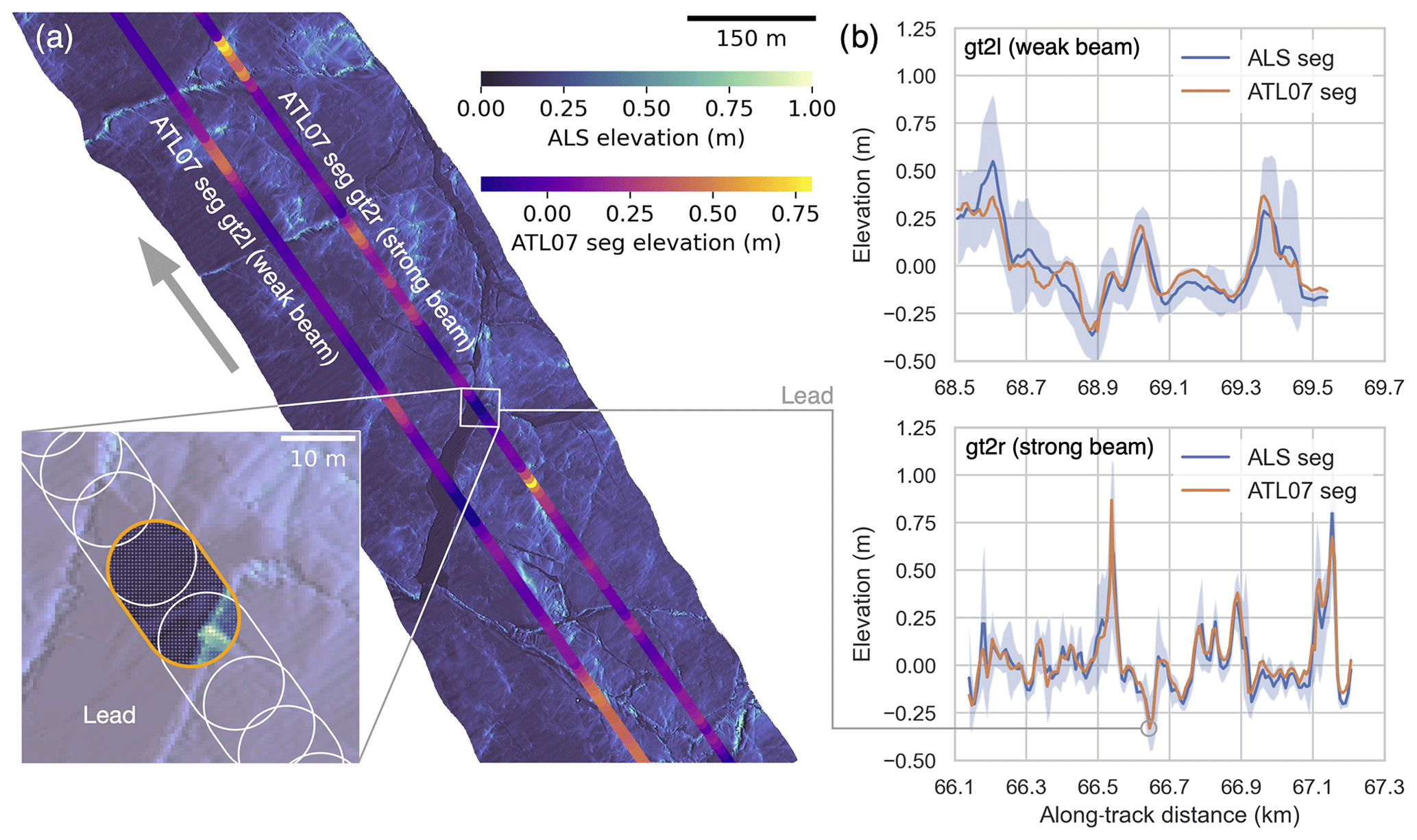
Figure 2 (a) Profile section (1 km) of the airborne laser scanner (ALS) swath with overlapping ICESat-2 beams after drift correction. The zoomed-in box shows the ICESat-2 segment outlines in white and one segment highlighted in orange, with matching ALS point measurements inside, corresponding to a lead. The gray arrow indicates the flight direction of the helicopter. (b) Elevation profiles, along the overlap shown in panel (a), of ICESat-2 beams and coincident ALS elevation, averaged within the corresponding ICESat-2 ATL07 segments. The blue shaded area in the elevation profiles represents the standard deviation of ALS point measurements within segments.

Figure 2 shows an example of a 1 km profile section, where the two ICESat-2 center beams gt2r and gt2l are overlapping with the laser scanner swath. The zoomed-in figure shows the ATL07 segment polygons of gt2r, which are overlapping each other, with a typical distance of 6–7 m between the segment centroids. For one of the segments, the assigned laser scanner points are shown.

If ATL07 segments are covered twice, on the outbound and return flight, the outbound flight is prioritized, and ALS measurements from the return flight are not considered for co-registration. We calculate an along-track distance that starts at zero – the time when the first overlap between ALS and ATL07 is registered. The along-track distance is also continued after the turning point. Therefore, ATL07 segments that are only covered during the return flight appear towards the end of the profile when referring to the along-track distance. Figure 1b shows co-registered ALS points after the turning point that fill a gap at the beginning of the outbound flight.

The UMD-RDA product is included in the co-registration of ATL07 and ALS by evaluating the timestamps of UMD-RDA and co-registered ATL07.

2.4 Drift correction

Due to the time difference between ALS and ICESat-2 observations, the co-registration of ICESat-2 and ALS measurements is affected by the drift of the sea ice. From observations at RV Polarstern and evaluation of the Ocean and Sea Ice Satellite Application Facility (OSI SAF) low-resolution ice drift product (Lavergne et al., 2010), we know that ice drift was rather weak in the region, with magnitudes of 0.01–0.02 m s⁻¹ in the southerly direction (Fig. 1a). However, even under such conditions, expected offsets will be up to ∼ 70 m, assuming a maximum delay of about 60 min. Considering the sampling rates and spatial resolution of ALS and ICESat-2 (Sect. 2.1 and 2.2), the need for ice drift correction becomes apparent. To evaluate and correct the effect of ice drift in between helicopter and satellite data acquisitions, we calculate correlations between ATL07 segment elevations and segment-averaged ALS elevations after incrementally applying drift corrections to the original ALS point measurements before co-registration in steps of 0.005 m s⁻¹ in both the x and y directions of the polar stereographic projection axes. Figure 3 shows two examples of correlation coefficients between ATL07 segment elevations and segment-averaged ALS elevations after applying a set of a priori assumed drift components on an ALS data frame. Here, we assume a range of sea ice drift velocities between −0.04 and 0.04 m s⁻¹ in each direction. The correlation analysis shows that, in the case of a 30 s data frame from 31 min before the rendezvous point, a maximum correlation of 0.87 is reached with a sea ice drift of 0.02 m s⁻¹ in the x direction and −0.015 m s⁻¹ in the y direction. Similarly, for the second example, where correlations are generally higher, we find a maximum correlation of 0.92 with sea ice drift of 0.02 m s⁻¹ in the x direction and −0.005 m s⁻¹ in the y direction. With this method applied to every 30 s ALS data frame, we find sea ice drift velocities ranging between 0.014 and 0.02 m s⁻¹, which corresponds well to the OSI SAF low-resolution drift product (Fig. 1a). Due to the choice of 0.005 m s⁻¹ binning, we expect uncertainties in the x and y directions of at least 0.0025 m s⁻¹.

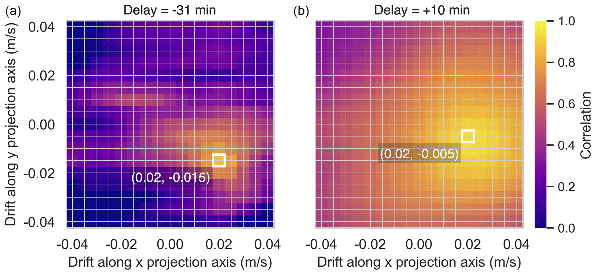
Figure 3 Evaluation of sea ice drift correction for two different airborne laser scanner (ALS) data frames from (a) 31 min before the rendezvous point and (b) 10 min after. The Pearson correlation between ALS and ICESat-2 segment elevations for applied sea ice drift in steps of 0.005 m s⁻¹ in the x and y directions of the polar stereographic projection. White squares highlight sea ice drift in the x and y directions, where the maximum correlation between ALS and ICESat-2 segment elevations is achieved.

2.5 Removal of undulations due to poor Global Positioning System (GPS) solution in ALS data

Mainly due to the poor GPS solution close to the North Pole, the entire ALS profile reveals undesired undulations and erroneous gradients in the along-track direction in the ALS elevations of up to several meters in magnitude (Fig. 1b). These need to be corrected. We first detect gaps in the elevation profile, caused by missing overlap between ALS and ICESat-2, and then divide the profile into segments that are free of gaps. To correct each profile segment for erroneous gradients, we apply a moving Gaussian window of 5 km length along each profile segment and remove the obtained low-pass-filtered signal from the original data. The choice of the 5 km window length is supported by findings during the processing in Hutter et al. (2022) which showed that most of the variability is caused by undulations at scales of 5 km and larger. Finally, we concatenate the individual profile segments to receive the corrected ALS elevation profile. We note that this correction will also eliminate natural long-wave signals and gradients from the ALS profile, and the freeboard estimation will be corrupted. However, as we only consider the surface topography in this study, removal of long-wave signals does not affect our analysis. For conformity, this correction is also applied to ICESat-2 data, including ATL07 seg and UMD-RDA. Consequently, all elevation products after this correction are referenced to the low-pass-filtered surface elevation.

2.6 Mapping of obstacles and their dimensions

To evaluate how well ATL07 seg and UMD-RDA are able to map the surface topography and dimensions of features, we apply a peak detection algorithm. Our method is based on the find_peaks function as part of the Python scipy.signal signal processing library. The function locates local maxima and calculates the height of the peak, which is defined as the height of an obstacle above the local level sea ice in this work. From a given peak, we evaluate if a virtual horizontal line intersects the slope of another peak on the left or right within a given maximum distance of 250 m to either side. This value has proved reasonable after empirical evaluation using different values. Either within the maximum distance or until the next peak, we search for the minimum on either side of the peak. The higher value then represents the elevation of the local level sea ice. The height of an obstacle is calculated as the vertical difference between the peak elevation and the elevation of the local level ice. To be classified as an obstacle, this difference must exceed 0.6 m (Hibler et al., 1972; Duncan et al., 2018). The minimum distance between two neighboring peaks is set to 16 m, which is approximately 2 times the distance between the centroids of two subsequent ATL07 segments. This method also complies with the Rayleigh criteria: two maxima points must be separated by a point with a height smaller than half of the maxima to be resolved as separate features (Hibler, 1975; Castellani et al., 2014). Here, we apply a stricter criterion, because we use high-resolution data. For example, in the case of two peaks separated by a point with lower elevation, the Rayleigh criterion is met as described above. When using high-resolution data, like ALS full or UMD-RDA, with point spacing <1 m, we assume that these two peaks belong to the same surface feature, whereas only one would be registered using our stricter method.

We also estimate the widths of obstacles. The height of the obstacle is halved and subtracted from the peak elevation. At the resulting height, a horizontal line is drawn, and the width of an obstacle is then given by the distance between the intersections of the line with the slope on either side of the peak. The lower limit for estimated widths is 1 m. The spacing of obstacles is given by the along-track distances between consecutive obstacles.

3 Results

3.1 Comparison between ATL07 and ALS co-registered elevations

For the entire profile of co-registered data, Fig. 4a visualizes the height distributions, which are divided into the weak beam gt2l and the strong beam gt2r. Here, we consider three different data sets (as introduced in Sect. 2.3): ALS seg, ATL07 seg, and ALS full. All three data sets reveal a lognormal-like distribution with a long tail towards higher elevations. Comparing strong and weak beams, we find that the gt2r (strong-beam) distribution shows a higher dynamic range for both ALS seg and ATL07 seg than for gt2l (weak beam), as indicated by the standard deviations of 0.23 m for ALS seg (gt2r) and 0.21 m for ATL07 seg (gt2r), compared with 0.18 m for ALS seg (gt2l) and 0.16 m for ATL07 seg (gt2l). Moreover, the gt2r distributions contain a larger fraction of high elevations. ALS seg (gt2r) and ATL07 seg (gt2r) contain 3.8 % and 3.3 % of elevations >0.5 m, respectively, whereas ALS seg (gt2l) and ATL07 seg (gt2l) only contain 2.0 % and 1.4 % of elevations >0.5 m, respectively.

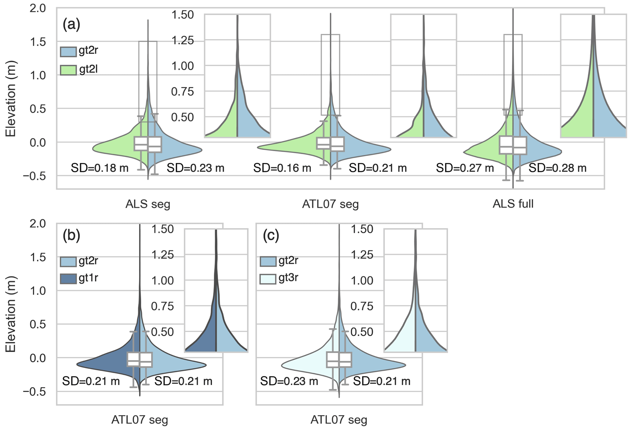
Figure 4 (a) Violin and box plots showing the elevation distributions from the segment-averaged ALS elevations (ALS seg), ATL07 segments (ATL07 seg), and the ALS elevations from all co-registered points at a 50 cm resolution (ALS full), separated between weak (gt2l) and strong (gt2r) beam segments. (b) Violin and box plots showing the elevation distribution of the strong beams of beam pair 2 and 1. (c) Violin and box plots showing the elevation distribution of the strong beams of beam pair 2 and 3.

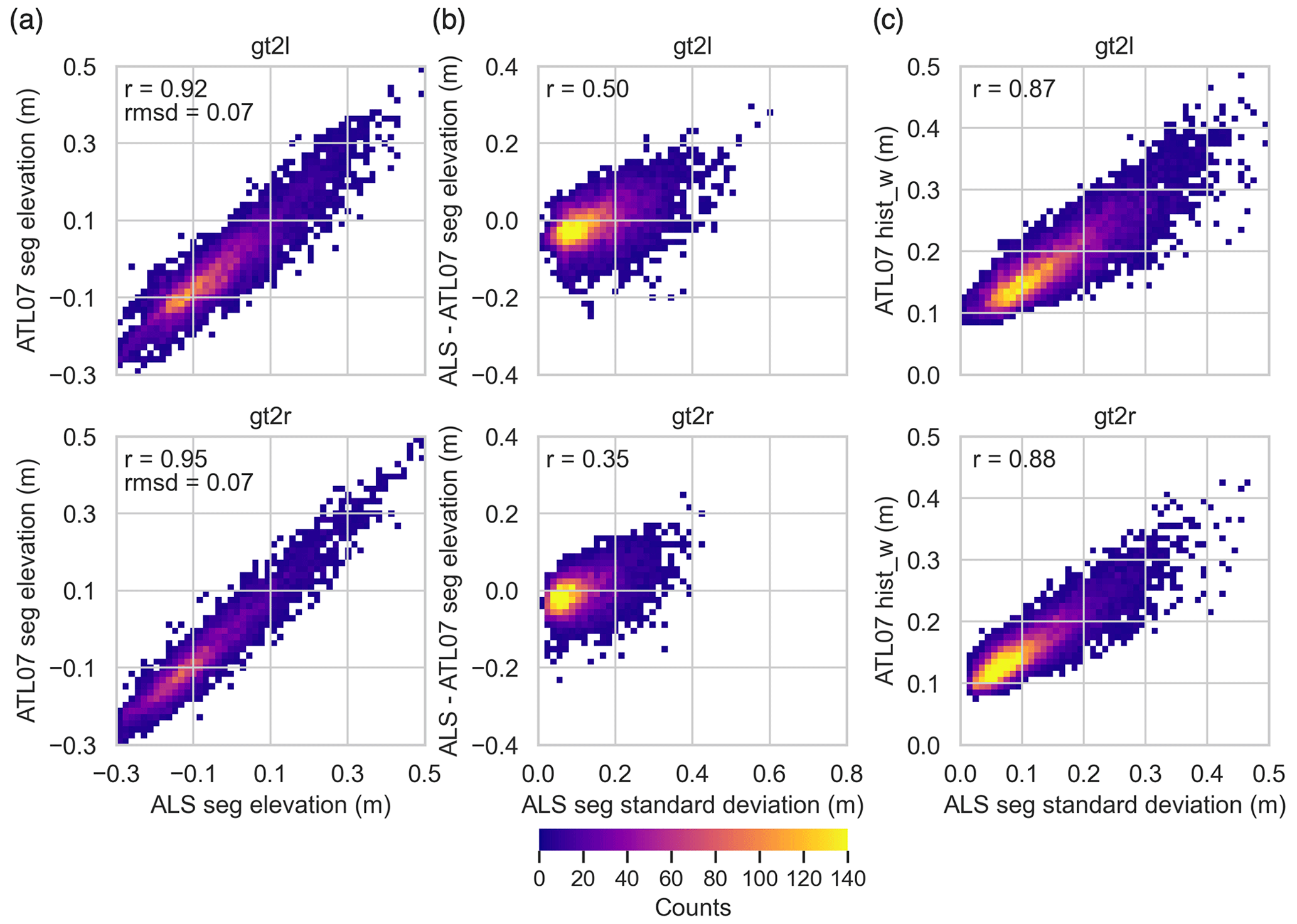
Figure 5 Scatterplots of co-registered ALS and ATL07 elevations: (a) comparison of segment-averaged elevations, showing the root-mean-square deviation (rmsd) and the Pearson correlation coefficient (r); (b) comparison between the ALS segment standard deviation and the difference between ALS and ATL07 segment elevations; and (c) comparison between the ALS segment standard deviation and ATL07 hist_w, representing the width of the height distribution within segments, provided in the ATL07 data product. Note that the rmsd refers to the elevations after subtraction of the long-wave correction (Sect. 2.5).

Considering ALS full, the distribution reveals a significantly higher fraction of elevations >0.5 m (5.3 % for gt2r) compared with ALS seg and ATL07 seg as well as a generally higher dynamic range, with standard deviations of 0.28 m and 0.27 m for gt2r and gt2l. In contrast to ALS seg and ATL07 seg, gt2l and gt2r distributions of ALS full reveal a similar dynamic range.

To illustrate how representative the results in this study are of the surrounding ice conditions, we compare gt2r with the statistics for the outer strong beams gt1r (Fig. 4b) and gt3r (Fig. 4c). We find similar elevation distributions with standard deviations of 0.21 m and 0.23 m for gt1r and gt3r, compared to 0.21 m for gt2r.

Considering the along-track signal, Fig. 2b shows the elevations of ALS seg and ATL07 seg along a 1 km profile section. In general, ALS seg and ATL07 seg reveal a similar variability and good agreement, even on small scales, but the gt2r profiles reveal a higher dynamic range, higher amplitudes, and generally more variation than the gt2l profiles. The agreement between ALS seg and ATL07 seg is also shown in Fig. 5a, which presents a comparison between all co-registered elevations of the entire helicopter flight. The Pearson correlations between the segment-averaged ALS elevations and corresponding ATL07 elevations are 0.92 for gt2l and 0.95 for gt2r. The root-mean-square deviation (rmsd) values are 0.07 m for both gt2l and gt2r. Here, we acknowledge that the value of the rmsd is limited by the fact that we have subtracted a long-wave signal from the elevation data sets; therefore, the rmsd does not relate to the heights of the original data sets.

The relationship between surface roughness and retrieved segment-scale elevations is assessed in Fig. 5b, where we consider the standard deviations for all ALS elevation points within each segment and compare them with the elevation difference between ALS seg and ATL07 seg. This indicates how the ATL07 product is affected by surface roughness within the segments. For both beams, the difference distributions are slightly skewed, with correlations of 0.5 and 0.35 for the gt2l and gt2r beams, respectively.

Figure 5c compares the standard deviations for all ALS elevation points within each segment with ATL07 hist_w from the individual photons within each ATL07 segment, given in the ATL07 product. Here, we find a Pearson correlation of 0.87 for gt2l and 0.88 for gt2r. This shows that the individual photon heights that are used to calculate the ATL07 segment heights can reproduce the actual surface roughness within the segments to a certain degree. In Sect. 3.4, we will see that an advanced evaluation of individual photon heights derived from ATL03 (UMD-RDA) is capable of capturing high-fidelity surface topography features at the meter scale.

In the following section, we investigate in more detail how surface roughness is represented in the ATL07 segments.

3.2 Comparison between ATL07 and ALS within segments

This section utilizes the high-resolution photon elevations that make up each ATL07 segment for a comparison with ALS elevations within these segments.

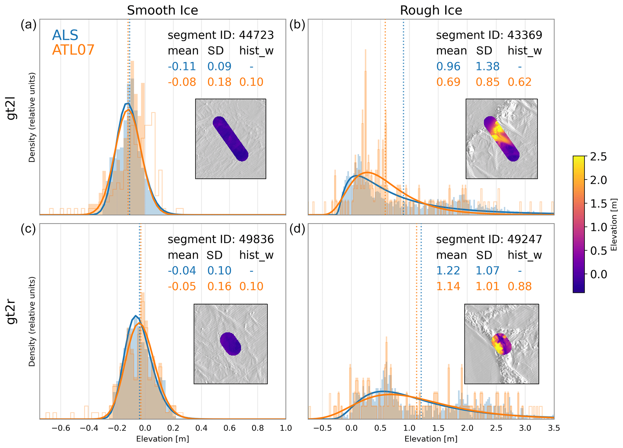
Figure 6 Example ATL07 segments and photon heights that comprise each segment, compared with ALS within-segment elevations. Example segments are chosen to represent relatively smooth ice (a, c) and rough ice (b, d) from the weak beam gt2l (a, b) and the strong beam gt2r (c, d). The orange histograms (bars) show the elevation distributions from the ATL07 segment, where the filled bars give the trimmed histogram used to derive elevation in the ATL07 product and the unfilled bars give the entire, non-trimmed photon histogram (defined in Sect. 2.2). The associated within-segment ALS elevations are shown as filled blue bars. Bin sizes are 2.5 cm for all examples. The trimmed ATL07 and ALS histograms are fitted with a lognormal distribution (solid lines), from which the provided means and standard deviations (in meters) are drawn. The hist_w represents the width of the height distribution within segments in the ATL07 product. Inset plots show the within-segment ALS elevations highlighted on top of the surrounding ALS ice elevations (shown using hillshading).

Figure 6 shows four examples of ATL07 segments and the photon height distributions that make up each segment as well as the corresponding ALS elevations from within the same segment. To compare the two data sets in light of sampling discrepancies (e.g., differences in sensor frequency and measurement counts within each segment), a lognormal distribution was fitted to both data sets, and statistics such as the mean, mode, and standard deviation were drawn from the modeled distributions. Over relatively smooth ice, the mean and standard deviation of the modeled fits for both ATL07 and ALS agree to within 1 cm across both beams. Additionally, the lognormal model fitted to the ATL07 photons has a standard deviation within 1 cm of hist_w, corroborating the roughness estimate given in the ATL07 product. Over rough ice, the within-segment agreement worsens, although the shapes of the distributions remain similar. Mean within-segment elevation differences are ∼ 10 cm (∼ 30 cm) for the strong (weak) beam, and standard deviations differ by between ∼ 13 cm (strong beam) and ∼ 80 cm (weak beam). As seen in the smooth ice examples, the standard deviations of the lognormal fits agree well with the given hist_w for both beams.

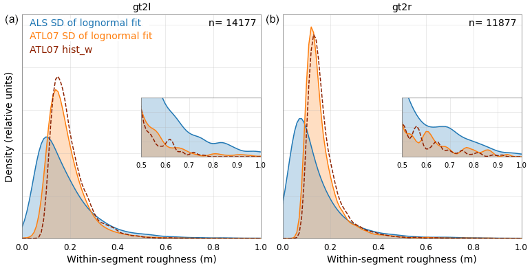
Figure 7 Probability density functions (PDFs) of roughness estimates from all overlapping segments for gt2l (a) and gt2r (b). Filled curves show the standard deviations of the lognormal fits to the within-segment elevation histograms from ALS (blue) and ATL07 (orange). The dashed red curve shows the ATL07 hist_w parameter, representing the width of the height distribution within segments. The inset axes highlight roughness values between 0.5 and 1.0 m.

While the examples shown in Fig. 6 demonstrate relatively good agreement between the ALS within-segment roughness (standard deviation of elevation measurements) and the ATL07 within-segment roughness (standard deviation of photon heights), this is not always the case across all overlapping segments. Figure 7 shows the distribution of roughness estimates in all segments, from ALS and ATL07, as well as the ATL07 hist_w. It is clearly seen that using the ATL07 heights to estimate roughness can miss the extremely smooth (<10 cm) and extremely rough (>40 cm) ice, resulting instead in more moderate (10–30 cm) roughness values. It is important to note that the differing system impulse responses from ALS and ICESat-2 are not accounted for in this analysis, which likely explains the observed differences over very smooth ice. Further explanations of these differences and their potential impacts are given in Sect. 4.3.

3.3 Occurrence of leads in ATL07 and ALS

During this underflight of ICESat-2 by ALS, no leads were identified in the ATL07 weak-beam (gt2l) data product, and only one lead was identified in the ATL07 strong-beam (gt2r) data product. Figure 8 shows this lead detected from beam gt2r as well as the leads detected from ALS along a ≥7 km section of the profile. In addition to the location of the leads, the ATL surface height profile (Fig. 8a) and one lead characteristic parameter for each sensor are given: the photon rate from ATL07 (Fig. 8b) and the surface reflectance from ALS (Fig. 8c). These parameters are used in the respective lead detection algorithms and are shown here to help to identify potential leads that are missed in the classification in the ATL07 product.

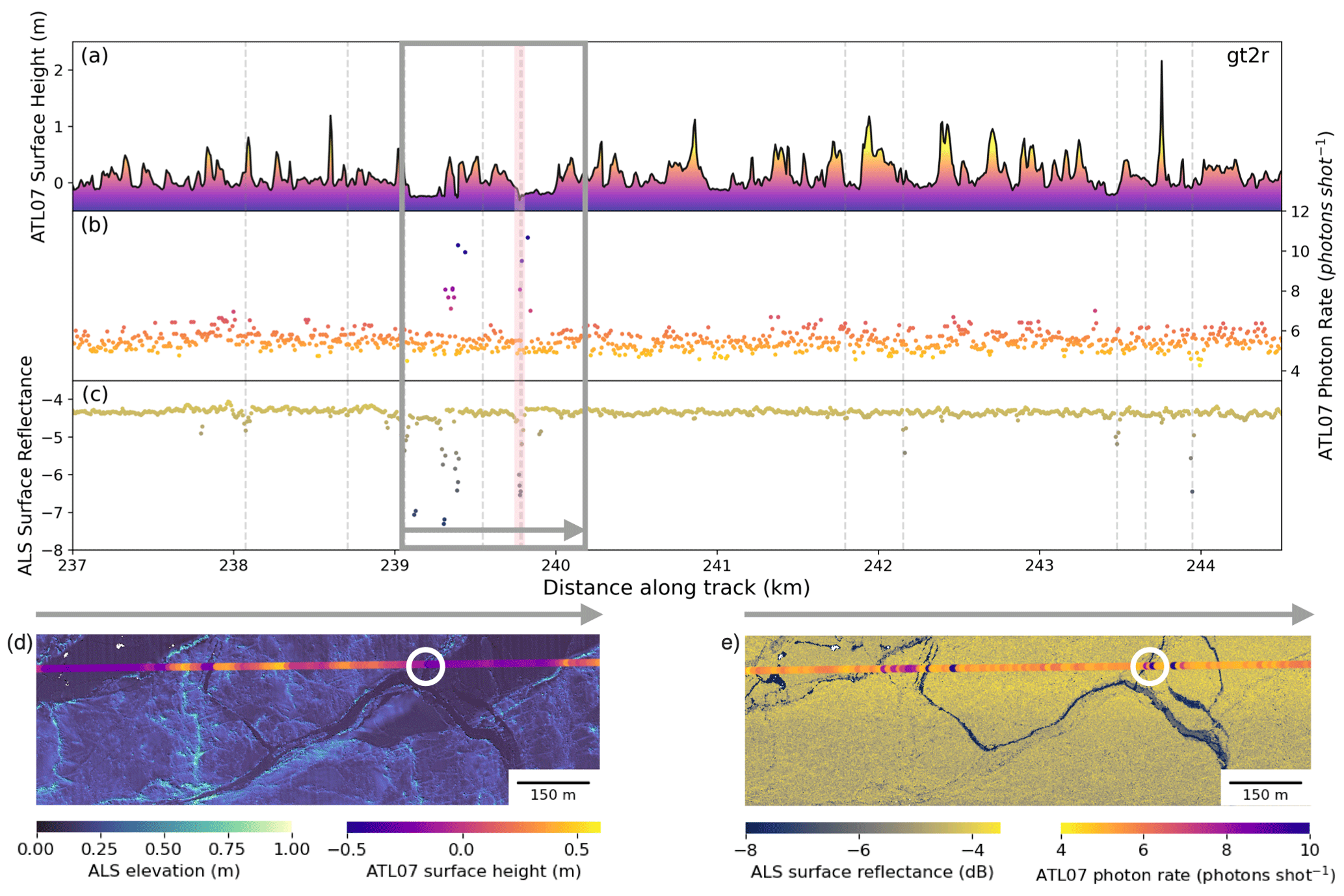
Figure 8 A ≥7 km section of the overlapping flight path with leads detected from ATL07 gt2r (vertical pink line) and from the ALS (vertical dashed gray lines). The three line profiles show the ATL07 height profile colored by elevation (a), ATL07 photon rates (b), and ALS surface reflectance (c). In panels (b) and (c), darker points represent values more probable to be classified as leads. The gray outlined box indicates the length of the subsections showing the gridded ALS elevations and coincident ATL07 gt2r elevations (d) as well as the gridded ALS surface reflectance and coincident ATL07 photon rates (e). The gray arrow indicates the flight direction. White circles highlight the only registered lead in ATL07.

The lone lead detected in the ATL07 gt2r data occurs near 239.75 km in the along-track direction and can be corroborated by the co-located height minimum and the local maximum in the photon rate. The narrow drop in ATL07 heights suggests a relatively small, specular lead. The ALS also records a lead in the same location, indicated by a drop in the surface reflectance. The ALS elevation model (Fig. 8d) and the ALS surface reflectance (Fig. 8e) show a system of narrow, partly open cracks within older and larger, refrozen leads in the vicinity of the detected lead in ATL07. In total, ALS detects 10 leads over this profile section. Some of the leads detected from ALS appear to be missed in ATL07, such as those occurring at about the 243.5 and 244 km marks in the profile. These locations both show a relative minimum in the surface height and a minimum in the ALS surface reflectance indicative of a lead, although one shows a small peak in the ATL07 photon rate whereas the other shows a local minimum. Possible explanations for these missed leads are discussed in Sect. 4.2.

3.4 Detection of obstacles using different ICESat-2 products

In this section, we investigate the capabilities of ATL07 seg and the UMD-RDA high-fidelity product to detect ridges and measure their sail heights. We use ALS full as the reference, as it provides a point spacing of 50 cm, which is assumed to represent the true surface topography along the ICESat-2 beams. In addition, we will also consider ALS seg. We use the term “obstacle” for topographic features, including pressure ridges, but also for fragments in rubble ice fields. Figure 9a shows a 500 m profile section for the strong beam gt2r. Here, elevations are referenced to the level ice. This profile section contains flat, level ice but also deformed sea ice with elevations of up to 1.5 m. While ALS seg and ATL07 seg show a smooth elevation profile, resulting in a reduced dynamic range and missing peaks, UMD-RDA can also resolve steep slopes and smaller details of the surface, e.g., at 89.25 km (Fig. 9a). However, UMD-RDA cannot resolve all of the peak heights given by ALS full. Within the 500 m section, seven obstacles with heights of 0.6 m above the local level ice are detected in ALS full. On the other hand, we find three obstacles in UMD-RDA and only one in ATL07 seg and ALS seg. Figure 9b shows the statistics of obstacle detection for the entire flight profile. In total, 532 obstacles are detected within ALS full, 225 are detected in UMD-RDA, 87 are detected in ATL07 seg, and 102 are detected in ALS seg. The shape of the density distribution of detected obstacle heights is similar among all products, but heights >1.8 m are sparse in ATL07 seg and ALS seg. The distribution of obstacle widths reveals a mean of 7.7 m for ALS full, whereas average widths are 39.6 and 38.4 m for ATL07 seg and ALS seg, respectively. The widths of the UMD-RDA obstacles are in between these values (24.4 m). The spacing between obstacles is a consequence of the detection counts; therefore, we find the lowest spacing for ALS full, whereas ATL07 seg and ATL07 seg show the highest spacing.

Figure 9 (a) The 500 m profile section along strong beam gt2r with sea ice elevations of different height products. Filled circles highlight peaks that exceed a height of 0.6 m with reference to the modal elevation of the entire track. The contour in the background shows the actual topography from airborne laser scanner (ALS) data along the center line of the ALS gridded segments shown at the top, corresponding to the ATL07 segment area. (b) Distributions of properties of n detected peaks (> 0.6 m) along the entire helicopter profile: heights and widths of obstacles as well as spacing between obstacles. μ represents the mean value for each distribution.

Figure 10 The same as Fig. 9 but for the weak beam gt2l.

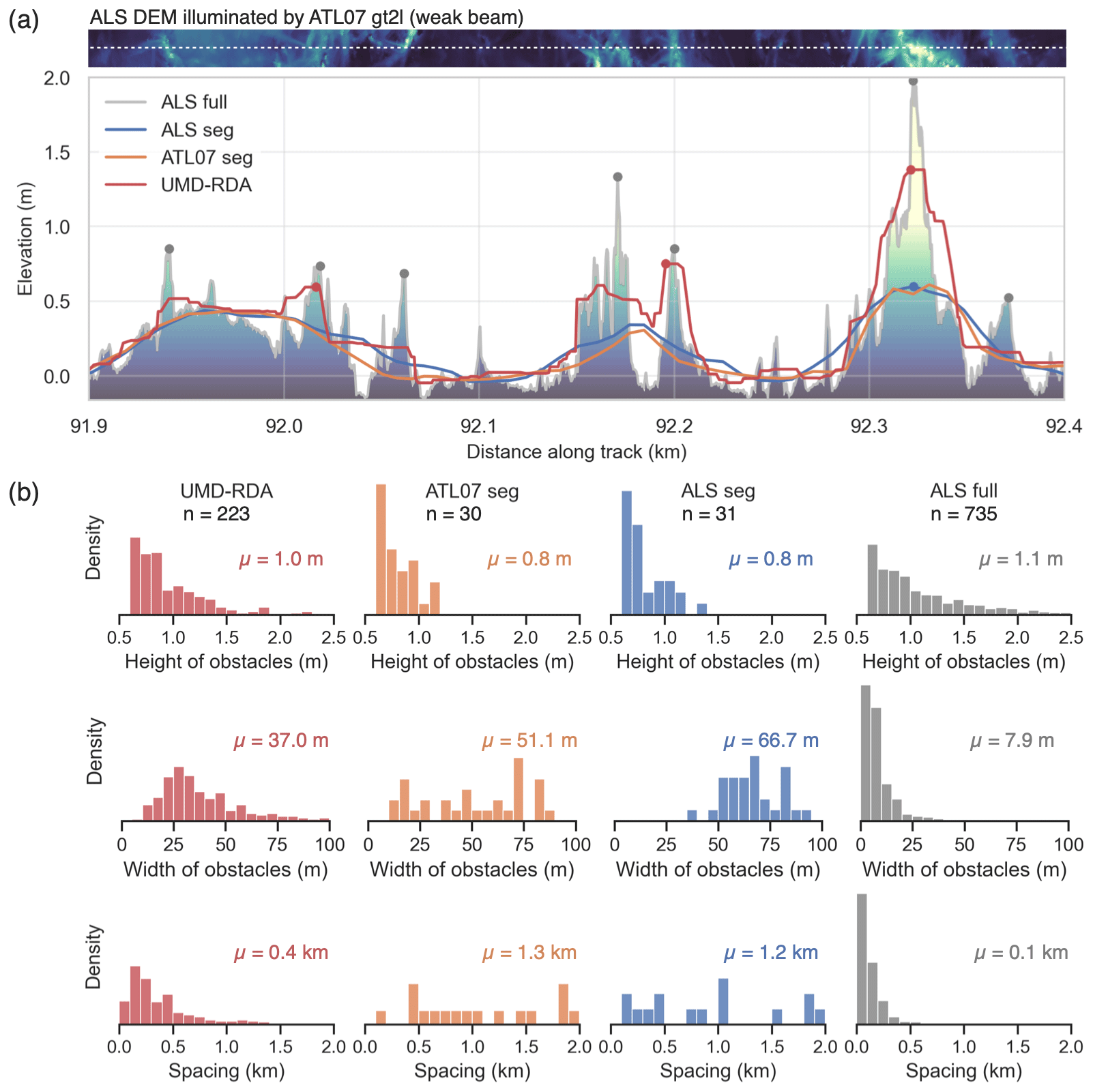
The same analysis is done for the weak beam gt2l (Fig. 10). Due to the longer segments, the elevation profiles of ALS seg and ATL07 seg appear even smoother compared with ALS full (Fig. 10a). In contrast, UMD-RDA is still able to resolve some of the peaks. This is also reflected in the profile statistics (Fig. 10b). In ATL07 seg and ALS seg, only 30 and 31 obstacles that exceed the 0.6 m height threshold are registered, respectively. In UMD-RDA, 223 obstacles are detected, whereas ALS full reveals 735 detected obstacles. Distributions for widths and spacing are similar to gt2r but with higher mean values for ALS seg, ATL07 seg, and UMD-RDA.

4 Discussion

4.1 Differences between weak and strong beams

The differences between the weak and strong beams are a result of the surface reflectance and laser power. The laser power of the strong beams is about 4 times greater than that of the weak beams. Therefore, for the data set used here, segments of the weak beam are about 3.5 times longer in order to collect the 150 signal photons, but the segment spacing is comparable (Markus et al., 2017). This results in smoother elevation profile for the weak beam (Fig. 2), whereas the strong beam reveals more details of the surface topography. However, when comparing the aforementioned elevation profiles to segment-averaged ALS elevations, we find that the performance of the weak beam is comparable to the strong beam with respect to the correlation and rmsd values (Fig. 5). Thus, weak-beam elevations are suitable for large-scale studies of the sea ice freeboard and thickness, when small-scale topography is less important. However, for the estimation of freeboard, information about the sea level is required. In the next section, we therefore discuss the presence of leads in the ICESat-2 ATL07 product, compared with leads detected in the ALS data.

4.2 Leads in ATL07

The conversion from sea ice elevation to the sea ice freeboard – and subsequently to sea ice thickness – is reliant on having observations of the local sea surface from leads in the sea ice, which must be within a reasonable vicinity of the sea ice elevation measurements (commonly between 10 and 200 km; Kwok et al., 2022). The number of sea ice leads is an important factor in the sea ice freeboard computation, and having more observations of sea surface heights from leads decreases the overall uncertainty (Di Bella et al., 2018; Ricker et al., 2016). ICESat-2, which provides altimetry data of higher spatial resolution than previously seen, allows for the measurement of narrower leads than previously possible, thereby increasing number of estimates of the local sea surface height. However, the requirement of having enough photons to produce one sea ice elevation measurement also applies for estimations of sea surface elevations in leads. Similarly, sensing the sea surface depends on the reflectance and specularity of the surface as well as the number of detected photons. Therefore, while more leads may be observable from ICESat-2, based on the current ATL07 retrieval methodology of having to rely on 150 photons to create one segment, it is likely that not all of the leads nor the entirety of each lead will be detected. This is a risk that will likely be more prevalent for the weak beams, as fewer photons are detected.

Figure 8 illustrates the limitations of ATL07-identified leads. While the segment is relatively short (7 km), only 1 of 10 leads identified in ALS was also identified in ATL07. This contrast between ALS-identified leads and ATL07-identified leads is remarkable. From the ATL07 photon rate and surface height, we observe potential leads that were not classified as such, including those between kilometers 243 and 244. It is likely that this discrepancy and non-classification are due to multiple factors. For one, the leads observed along this profile are mostly very small (only few meters wide), refrozen cracks in the ice (Fig. 8d, e). These cracks are smaller than the ICESat-2 footprint and much smaller than the 150-photon-aggregate segments; therefore, the elevations and photon rates get smoothed by the surrounding ice floes and do not meet the threshold criteria to be considered a lead. Additionally, ATL07-classified lead returns are expected to be specular or quasi-specular, i.e., leads with smooth surfaces, as shown by the increase in photon rates in Fig. 8b (Kwok et al., 2021b). The current algorithm for ATL07 does not consider “dark leads” (i.e., drops in the photon rate) in the classification procedure (Kwok et al., 2022). The potential lead around 244 km, for example, appears to show a local minimum in the photon rate, which could signal a dark lead that was not classified.

With the higher resolution of UMD-RDA, the edges of leads are more likely to be detected with higher precision due to less smoothing, which will provide more precise estimates of the width of the detected leads. ATL07 seg is likely to smooth the lead edges due to the 150-photon-aggregate requirement, leading to a larger minimum detectable width of the detected leads in the ATL07 product, where lead detection is based on a radiometric classification (Kwok et al., 2021b). However, with the higher along-track resolution of UMD comes a detectable rougher surface in the open leads compared with the smoother ATL07 leads, due to a lower photon signal-to-noise ratio. As the UMD algorithm aims to measure the top of the sea surface, there is the possibility of obtaining a higher estimate of surface elevation within a lead compared with ATL07 seg. However, as UMD also aims to measure the tops of obstacles at the sea ice surface, this effect is likely to be mitigated when converting to the freeboard.

Another aspect that adds to the discrepancies in Fig. 8 comes from the fact that the ALS swath is wider than the ATL07 segment width (Fig. 8d, e) and that the ALS lead-finding procedure incorporates returns from outside of the overlapping segments. Future analysis of overlapping profiles that flew over more, open, and larger leads would be better to assess the ATL07 parameter lead thresholds and determine the minimum detectable width of leads. Additionally, a future modification to the ATL07 algorithm could be implemented that, for example, relaxes the 150-photon requirement for leads, as fewer signal photons should be needed to get an accurate height retrieval over flat surfaces.

4.3 How are ATL07 heights affected by surface roughness within segments?

The signal photon aggregates used to estimate surface height in ATL07 also provide information related to the surface topography within each segment. By analyzing the photon height distributions (Fig. 6), we get a sense of the roughness of the within-segment surface. While these roughness estimates, given as the standard deviation of the lognormal fit or the hist_w parameter, generally correlate with that from ALS ($r=\mathrm{0}.$87–0.88; Fig. 5c), it is shown that they tend to overestimate the roughness of the smoothest ice and underestimate the roughness of the roughest ice (Fig. 7). This discrepancy is likely due to several reasons. It is likely that the differences in surface roughness that we see over smooth ice in Fig. 7 are a direct result of the different impulse responses between ALS and ICESat-2. Over rougher ice, where the impulse responses would have less of an impact, it is likely that the ATL07 photon aggregation and histogram trimming play a role in the discrepancy with respect to ALS. For a given 150-photon segment, the height uncertainty increases as the roughness increases, which could explain some of the observed differences in Fig. 6. Additionally, histogram trimming could remove the highest and lowest elevations from the distribution, effectively reducing its roughness, which could explain the differences in Fig. 7 at standard deviations greater than around 0.4 m.

In order to fully reconcile the retrieved within-segment elevations and roughnesses as well as to enhance confidence in the ATL07-derived roughness, a more robust analysis involving the system impulse responses and the ATL03 photon data aggregated to varying resolutions would be required. Additionally, future work involving the ATL07 algorithm (and specifically investigating the photon aggregation lengths, histogram-trimming procedure, and the dual-Gaussian assumed surface) would be useful to better understand how to capture the sea ice topography at these scales. Until such work is undertaken and due to the current discrepancies in the roughness estimates, we use only the high-resolution within-segment ALS elevation measurements to estimate roughness (as opposed to the ATL07 hist_w) and to help assess the impact of roughness on the returned ICESat-2 photon distribution and retrieved ATL07 heights.

If rougher sea ice had no impact on the retrieved ATL07 heights, we would expect Fig. 5b to show counts that were evenly distributed along the x axis with no correlation, as any differences in elevation between ALS and ATL would not be related to roughness. However, there is a skewness to the distributions, with a tail that extends towards positive elevation differences at larger roughness values. These distributions indicate that ATL07 heights tend to underestimate the surface elevation over rougher sea ice compared with ALS. This fact can be observed in Fig. 6b and d, as the mean value of the fitted lognormal distribution from ATL is less than that of ALS. It is possible that the trimming of the histograms in ATL07 could play a role. When using the non-trimmed histograms, the ATL mean values of the fitted distributions are 0.7 m and 1.15 m, which are in slightly better agreement with ALS compared with the values in Fig. 6b and d, respectively. However, not trimming the histograms leads to worse lognormal fits overall and also means that anomalous photons could potentially be included in the elevation retrieval (Kwok et al., 2022). Future work on the histogram-trimming procedure and dual-Gaussian assumed distribution in ATL07 is needed to fully understand their impact on the retrieved elevations.

The lengths of the segments may also contribute to the underestimation of ATL07 heights from rougher segments. This is due to two main reasons. First, longer segments have a higher probability of encountering obstacles that increase the roughness compared with shorter segments. This is shown in Fig. 7, where gt2l records a lower density of very thin, level ice segments as well as a higher density of very rough ice segments compared with gt2r. Second, the longer segment would lead to more smoothing of the surface obstacles in the ATL07 heights, as the single ATL07 height estimate comes from a larger area, which results in an underestimation of the highest elevations. This smoothing is observed in Figs. 9 and 10 and is more pronounced in the longer-segment gt2l data. The combination of rougher segments and more pronounced smoothing seen in gt2l segments would suggest a larger impact of roughness on the ATL07 weak-beam elevations compared with the strong beam. Figure 5b confirms this hypothesis, as gt2l shows a higher correlation, indicating more of an impact, as well as a more skewed distribution with a longer tail.

4.4 Mapping of ridges with ICESat-2 products

Our results show that ICESat-2 allows for detection and height estimation of individual surface topography features. However, comparison with the high-resolution ALS data set also shows that not all ridges or obstacles will be captured. Ridge detection and sail height estimation depend on the applied algorithm, the dimensions of the ridge, and the data product used. In our study, we use a peak detection algorithm with a 0.6 m height threshold with respect to the surrounding level ice, similar to previous studies (e.g., Hibler et al., 1972; Tan et al., 2012; Duncan and Farrell, 2022). Lowering the threshold leads to more detection, whereas increasing the threshold results in a lower number of detections, following an exponential or lognormal function (Fig. 4).

Given the uncertainties in the geolocation of the ATL photon heights as well as uncertainties in the drift correction of at least 0.0025 m s⁻¹ in the x and y directions, we acknowledge potential uncertainties in our comparison due to the fact that we consider ALS full as a reference in this study. ALS full represents the elevations along a 0.5 m wide line through the center of the ATL-illuminated area, which is 13 m wide. As illustrated in Figs. 9 and 10, considering heights offset from the center by a few meters can lead to changes in the elevation profile and also in the detection statistics. However, as we consider a large number of points, we do not think that this affects the result of this comparison significantly.

Another aspect that is important for ridge detection is the ridge dimensions (in combination with the along-track resolution of the elevation data set). The segments in the ATL07 product reveal a typical spacing of 6–7 m, whereas the mean segment lengths are 17 m for the strong beam (gt2r) and 59 m for the weak beam (gt2l). Therefore, narrow but high obstacles with steep slopes are smoothed out in the ATL07 product. In contrast, high obstacles with a plateau are better represented in ATL07. This is shown in Fig. 9 between 89.35 and 89.4 km in the along-track direction, where a ridge with a width of about 30 m at mid-height is detected using the ATL07 product, whereas ridges with smaller dimensions are missed (for example at 89.25 km). Because of the longer segment length, this effect is stronger for the weak beam. Eventually, the smoothing also results in an underestimation of sail heights. In contrast to ATL07, UMD-RDA only uses five-shot aggregates and, therefore, achieves a higher along-track resolution, with an average point spacing of 0.7 m (1.8 m) for the strong beam (weak beam) found in this case study. Our work shows that using finer-resolution segments with fewer photons aggregated, such as the UMD-RDA product, can substantially improve ridge detection and sail height estimation over the coarser-resolution segments that aggregate more photons, such as the ATL07 product (Figs. 9, 10). If we consider ALS full as the reference, using ATL07 results in 16 % (4 %) of detected ridges for the strong (weak) beam. In contrast, using UMD-RDA, we obtain 42 % (30 %) of the detection number compared with ALS full. Interestingly, the level of relative improvement between UMD-RDA and ATL07 is even higher for the weak beam, decreasing by only 29 % with UMD-RDA but by 75 % with ATL07 with respect to the results with the strong beam.

While the height distributions of the detected ridges reveal similar shapes among all products, the width distributions differ substantially. The reason for this is that the width estimates strongly depend on the along-track resolution. The smoothing effect mentioned earlier leads to an increase in width, while narrow ridges with small widths (<5 m) can barely be detected with ATL07. Therefore, the width distribution is biased high.

The choice of segment length (ATL07 is of varying segment length using 150-photon aggregates, whereas UMD-RDA aims to provide observations on a per-shot basis) is also a choice made based on the overall objective of each algorithm. While ATL07 aims to provide observations of the average local sea ice elevation, UMD-RDA aims to sample the top of the sea ice pressure ridges. Therefore, UMD-RDA is more likely to provide higher estimates, as it is based on the 99th percentile of a trimmed five-shot aggregate applied on a per-shot basis (Farrell et al., 2020). However, it is notable that neither ATL07 nor UMD-RDA is capable of retrieving the full extent of the surface topography, such as capturing the full height of the obstacles or the depth of the topography (to a lesser extent for the strong beam) along the transects shown in Figs. 9 and 10. In the case of the weak-beam data, significant smoothing across deformation features is observed in ATL07 due to the longer segment lengths, whereas the UMD-RDA algorithm appears to overestimate local minima between obstacles along the transect. While this is a function of resolution, it is also due to the UMD algorithm aiming to obtain elevation estimates using the 99th percentile and, therefore, using the higher-elevation photons within the aggregates as a measure of the surface elevation.

The fact that neither ATL07 nor UMD-RDA is able to capture the full extent of the surface topography likely shows the limitations of ICESat-2 for specific obstacle detection. With that being said, considering that ICESat-2 is a spaceborne platform observing meter-scale features from a 500 km orbit, these results are remarkable if compared to previous satellite altimeter missions.

4.5 Possible limitations of the study

Finally, we discuss how representative this study is, considering that our data set only covers a distance of about 130 km. The sea ice in the surveyed area is a mix of scattered multiyear floes (e.g., the MOSAiC floe) and a larger part of first-year sea ice (Nicolaus et al., 2022). From local observations, we know that this area was subject to several deformation events at that time (von Albedyll et al., 2022). Although both ice types are present, neither very thick and old sea ice, such as that typically found north of the Canadian Archipelago, nor large areas of very young ice (<10 cm thick) were covered. The Sentinel-1 radar image (Fig. 1a) suggests that the surveyed ice is representative of the surrounding area. Considering the other two strong beams, we find similar elevation distributions and standard deviations for gt1r, gt2r, and gt3r (Fig. 1b, c), indicating that gt2r reveals a dynamic range between gt1r and gt3r. Therefore, we conclude that our findings represent sea ice typical of the central Arctic in spring and that our results are representative of the other beams. However, we note that the segment lengths and spacing vary between the beams and can affect the statistics.

We anticipate that over (even more) deformed and thicker sea ice, the performance differences in mapping the sea ice surface topography between UMD-RDA and ATL07 will be comparable or even higher than in our study. On the other hand, over newly formed, rather flat, thin ice, differences between UMD-RDA and ATL07 will be rather subtle.

The evaluation of signals from leads in ATL07 is limited due to the lack of larger open-water leads, as we would expect them at different times of the season and in other regions such as the marginal ice zone or the Beaufort Gyre.

5 Conclusions

During the MOSAiC ice drift experiment, we carried out laser scanner measurements with a helicopter that were coincident with the center beam pair of an ICESat-2 overflight in March 2020. We processed airborne gridded sea ice surface elevations along a swath width of about 300 m, at a spatial resolution of 0.5 m, with an overlap of 97 km for the strong beam gt2r and 117 km for the weak beam gt2l. This unique data set allows one to study the capabilities of ICESat-2 sea ice surface elevations in the Arctic winter period.

We found that both the strong and the weak beam of ATL07 seg (the operational sea ice height product provided by NASA) coincide with the corresponding segment-averaged ALS estimates (ALS seg), with correlations of 0.95 (strong beam) and 0.92 (weak beam) and a root-mean-square deviation (rmsd) of 0.07 m, which is consistent with the findings of Kwok et al. (2019a). However, surface roughness is smoothed out on length scales smaller than the segment lengths. This has implications for the detection of leads as well as for ridges and estimates of their sail heights.

Only one lead was identified by the ATL07 algorithm, which missed smaller, partly refrozen cracks that can be seen in the ALS data set. This is a consequence of the fact that 150 photons are required to build a segment, thereby resulting in small leads and cracks being overlooked. Aggregation of fewer photons for lead detection might improve the overall performance. However, we also acknowledge that the ALS data set is not representative of other Arctic regions with a higher lead frequency, like the marginal ice zone or the Beaufort Gyre. More research is required on how lead detection can be improved, especially for small leads. Therefore, additional validation data sets and complementing measurements, such as airborne thermal infrared imaging, would be useful.

To assess the potential of ICESat-2 data for mapping of ridges and sail heights, besides ATL07 seg, we also considered the high-fidelity sea ice elevation product (Duncan and Farrell, 2022) from the University of Maryland (UMD-RDA). Here, we observe that UMD-RDA captures more obstacles with higher ridge sails more comparable to the ALS product in full resolution (ALS full), which is assumed to represent the true surface topography. We find that 16 % (4 %) of the number of obstacles in the ALS data set are detected using the strong (weak) center beam in ATL07. A significantly higher detection rate of 42 % (30 %) is achieved when using the UMD-RDA product. On average, for the strong beams, the obstacle sail heights are of similar magnitude (1.1 m for ALS full, 1.0 m for UMD-RDA, and 0.9 m for ALS seg and ATL07 seg), whereas the width of the obstacles varies significantly. While ALS full observed a high variety of surface obstacles and the topography in high detail, neither ICESat-2 algorithm is able to capture the topography to the same extent. For the weak beams, the segment lengths of each sea ice height segment are longer due to fewer photons being transmitted and detected, causing ATL07 to miss most of the obstacle features. However, our study shows that, when utilizing the high-resolution of ICESat-2 (demonstrated here with the UMD-RDA product), it is possible to provide basin-scale measurements of surface roughness and sail heights, which can be used for estimation of drag coefficients and to aid ship routing through the Arctic, if the uncertainties and limitations of these products, revealed in this work, are taken into account.

Considering the performance of the weak-beam measurements, our results suggest that weak-beam heights are useful for large-scale studies of the sea ice freeboard and thickness, when small-scale topography is less important. While previous studies commonly used the strong beams (e.g., Petty et al., 2020), additionally using weak beams to derive Arctic and Antarctic sea ice freeboard and thickness maps might increase the actual area of sensed sea ice and decrease uncertainties in the gridded products because of the increased number of measurements.

ALS surveys were carried out during the entire MOSAiC drift, providing a unique data set of sea ice surface topography through a full seasonal cycle (Hutter et al., 2022). This study links the MOSAiC ALS measurements with ICESat-2 measurements from space in order to investigate the evolution of surface topography and deformation of the sea ice near the MOSAiC camp in the context of regional and Arctic-wide changes captured by ICESat-2.