the Creative Commons Attribution 4.0 License.
the Creative Commons Attribution 4.0 License.
 | 31 Mar 2023
Feasibility of retrieving Arctic sea ice thickness from the Chinese HY-2B Ku-band radar altimeter
Zhaoqing Dong
Lijian Shi
Mingsen Lin
Yongjun Jia
Tao Zeng
Suhui Wu
With the continuous development of the China ocean dynamic environment satellite series (Haiyang-2, HY-2), it is urgent to explore the potential application of HY-2B in Arctic sea ice thickness retrievals. In this study, we first derive the Arctic radar freeboard and sea ice thickness during two cycles (from October 2019 to April 2020 and from October 2020 to April 2021) using the HY-2B radar altimeter and compare the results with the Alfred Wegener Institute (AWI) CryoSat-2 (CS-2) products. We evaluate our HY-2B sea ice freeboard and thickness products using Operation IceBridge (OIB) airborne data and Ice, Cloud, and land Elevation Satellite 2 (ICESat-2) products. Finally, we estimate the uncertainties in the HY-2B sea ice freeboard and sea ice thickness. Here, we derive the radar freeboard by calculating the difference between the relative elevation of the floe obtained by subtracting the mean sea surface (MSS) height and sea surface height anomaly (SSHA) determined by an average of the 15 lowest points method. The radar freeboard deviation between HY-2B and CS-2 is within 0.02 m, whereas the sea ice thickness deviation between HY-2B and CS-2 is within 0.2 m. The HY-2B radar freeboards are generally thicker than AWI CS-2, except in spring (March and April). A spring segment likely has more floe points than an early winter segment. We also find that the deviations in radar freeboard and sea ice thickness between HY-2B and CS-2 over multiyear ice (MYI) are larger than those over first-year ice (FYI). The correlation between HY-2B (CS-2) sea ice freeboard retrievals and OIB values is 0.77 (0.84), with a root mean square error (RMSE) of 0.13 (0.10) m and a mean absolute error (MAE) of 0.12 (0.081) m. The correlation between HY-2B (CS-2) sea ice thickness retrievals and OIB values is 0.65 (0.80), with an RMSE of 1.86 (1.00) m and an MAE of 1.72 (0.75) m. The HY-2B sea ice freeboard uncertainty values range from 0.021 to 0.027 m, while the uncertainties in the HY-2B sea ice thickness range from 0.61 to 0.74 m. The future work will include reprocessing the HY-2B L1 data with a dedicated sea ice retracker, and using the radar waveforms to directly identify leads to release products that are more reasonable and suitable for polar sea ice thickness retrieval.
- Article
(9095 KB) - Full-text XML
- BibTeX
- EndNote


Arctic sea ice is an important factor in the global climate system and plays an important role in maintaining its energy balance. By reflecting most of the solar shortwave radiation, sea ice reduces the absorption of solar shortwave radiation by seawater and blocks outwards longwave radiation from leaving the ocean, thus regulating the overall radiation budget of the Earth. Sea ice also regulates the exchanges of heat, momentum and water vapour between the polar atmosphere and oceans (Thomas and Dieckmann, 2010; Xu et al., 2017). Due to the special air–ice–sea feedback mechanism, the Arctic has exhibited warming temperatures at more than twice the global average increasing rate. This phenomenon is known as “Arctic amplification” (Serreze et al., 2009). Studies have shown that global warming has led to decreases in the extent and thickness of Arctic sea ice and that the ice age of multiyear ice has gradually decreased (Comiso et al., 2008; Lindell and Long, 2016; Kwok, 2018; IPCC, 2022; Meier and Stroeve, 2022). Models predict that the Arctic will be ice-free in summer by the middle of the 21st century (Notz and SIMIP Community, 2020). The predicted decrease in Arctic sea ice will also change the living environment of Arctic mammals, and these changes will not be conducive to the survival or development of Arctic mammals, such as polar bears and walruses (IPCC, 2019). Due to the rapid retreat of sea ice, trans-Arctic shipping routes have become increasingly navigable (Stephenson and Smith, 2015; Cao et al., 2022). In addition, the reduction in Arctic sea ice has improved the convenience of exploiting natural resources in the Arctic, and these activities will have an important impact on the economy of the Arctic and on regions beyond the Arctic.
Sea ice thickness, as the third dimension of sea ice, can be combined with sea ice extent to calculate sea ice volume to better understand changes in sea ice. However, sea ice thickness is also a difficult parameter to measure. The recent development of satellite altimeters has made it possible to obtain sea ice thickness over continuous and large ranges. To date, the available international altimeter satellites that obtain polar sea ice thickness observations include the European Remote Sensing satellite 1 (ERS-1); ERS-2; Envisat; the Ice, Cloud, and land Elevation Satellite (ICESat); CryoSat-2 (CS-2); SARAL; Sentinel-3A; Sentinel-3B; and ICESat-2 (IS-2). Laxon et al. (2003) derived Arctic sea ice thickness for the first time with the ERS-1/2 altimeter and verified their findings with submarine sonar data, thus confirming the feasibility of using satellite altimeters to retrieve sea ice thickness. Kwok (2004) derived the Arctic sea ice thickness for the first time in 2004 using the Geoscience Laser Altimeter System (GLAS) on the ICESat satellite, further demonstrating the advantage of altimeter data in estimating Arctic sea ice thickness. Giles et al. (2008) estimated the Arctic sea ice thickness using the Envisat altimeter and analysed its variation pattern in winter from 2002 to 2007; the authors found that the area where the sea ice thickness showed a decreasing and thinning trend was mainly in the Beaufort Sea. Tilling et al. (2016) released near-real-time CS-2 sea ice thickness products with time periods of 2, 14 and 28 d. Additionally, based on CS-2 data, Ricker et al. (2014) set threshold ranges for the pulse peak (PP), stack standard deviation (SSD) and stack kurtosis (K) terms to separate the lead, sea ice and open water; compared and analysed the effects of different retracking thresholds on the sea ice thickness; and estimated the uncertainties of the sea ice freeboard and sea ice thickness. Shen et al. (2020) used Sentinel-3A to retrieve the Arctic sea ice freeboard and analysed the difference and consistency between Sentinel-3A and CS-2. The results showed that the Sentinel-3A sea ice freeboard was generally lower than that retrieved by CS-2. The differences between Sentinel-3A and CS-2 are mostly a result of the processing chain of Sentinel-3 not having included zero padding or Hamming weighting. The study of Lawrence et al. (2019), in which these processing steps were applied, showed greater consistency. Petty et al. (2020) generated monthly IS-2 sea ice thickness products and compared them with various monthly sea ice thickness estimates obtained from the European Space Agency's (ESA) CS-2 satellite mission, with IS-2 showing consistently lower thicknesses. With the continuous progress of Arctic sea ice remote sensing technologies, a wide variety of sea ice thickness products have become available to the scientific community (Sallila et al., 2019). CS-2 radar altimeters, ICESat and IS-2 laser altimeters cover almost the entire Arctic Ocean due to their large orbital inclinations and are thus the main data sources for estimating sea ice thicknesses. However, few reports have explored the retrieval of sea ice thickness by Chinese altimeters among recent studies of polar sea ice thickness. Jiang et al. (2022) preliminarily estimated the Arctic radar freeboard with HY-2B L1 from October 2020 to April 2021 and compared it with radar freeboard products from the Alfred Wegener Institute (AWI). They noted the average difference between Haiyang-2B (HY-2B) radar freeboard estimates and AWI data to be 0.088 ± 0.057 m. They generally observed higher radar freeboards for HY-2B than CS-2. Therefore, Jiang et al. (2023) used the AWI CS-2 sea ice thickness products to calibrate the HY-2B thickness estimates. With the continuous development of China's marine dynamic environment satellite, the feasibility of using the HY-2B satellite to map polar sea ice must be explored. It is important to note in this study, however, that we are aiming to investigate whether HY-2B can be used for sea ice but that we are limited to already provided higher-level (Sensor and Geophysical Data Record, SGDR) products and that it is not within the scope of the study to derive freeboard products using our own retracker from the HY-2B SGDR product.
In this study, we use the HY-2B radar altimeter to retrieve the Arctic radar freeboard and sea ice thickness and compare the results with the CS-2 products released by the AWI during the same period. Finally, we compare the results with Operation IceBridge (OIB) airborne data and IS-2 laser altimeter data. In Sect. 2, we introduce the data used in this study. In Sect. 3, we introduce the determination method of the sea surface height anomaly (SSHA) and the retrieval process of sea ice thickness in detail. In Sect. 4, we compare the Arctic HY-2B radar freeboard and sea ice thickness with AWI CS-2 products and IS-2 products. In Sect. 5, we discuss the influence of different SSHA determination schemes on the HY-2B radar freeboard and estimate the uncertainties in the HY-2B sea ice freeboard and sea ice thickness. Finally, in Sect. 6, we summarize the conclusions.
2.1 HY-2B radar altimeter
The HY-2B satellite was launched on 25 October 2018. It is China's second polar-orbiting marine dynamic environmental satellite and the second marine operational satellite in China's civil space infrastructure programme. Its main mission is to monitor and survey the marine environment and obtain a variety of marine dynamic environmental parameters, including sea surface winds, wave heights, sea surface heights, sea surface temperatures, and other elements, as well as the parameters of polar sea ice. The HY-2B satellite integrates both active and passive microwave remote sensors and carries loads such as a radar altimeter, microwave scatterometer, scanning microwave radiometer, correction radiometer, ship identification system and data collection system. The HY-2B satellite adopts an orbit with a repeat cycle of 14 d in the early stage and an orbit with a repeat cycle of 168 d in the late stage. Currently, the repeat cycle of HY-2B is 14 d. The HY-2B radar altimeter adopts the same reference ellipsoid as the TOPEX/Poseidon and Jason-1/2/3. The HY-2B radar altimeter is a dual-band pulse-limited radar altimeter that comprises the Ku band and C band to remove the impacts of ionospheric delays. Table 1 lists the main parameters of the HY-2B radar altimeter (Jiang et al., 2019; National Satellite Ocean Application Service, 2019).

The National Satellite Ocean Application Service (NSOAS) has released level-1, level-2 and fusion data products compiled through the preprocessing, data retrieval and statistical averaging of the HY-2B altimeter level-0 data. The level-2 products are divided into Interim Geophysical Data Records (IGDRs), SGDRs and Geophysical Data Records (GDRs). The SGDR products contain waveform data and have been retracked using the Brown model (Zhang et al., 2022). The HY-2B altimeter will switch between suboptimal-maximum-likelihood-estimation (SMLE) tracking mode and offset-centre-of-gravity (OCOG) tracking mode according to terrain changes. The SMLE tracking mode is suitable for areas with slower changes in terrain height, such as ocean and large areas of flat sea ice. The OCOG tracking mode is used for areas with dramatic changes in topographic height, such as land and sea ice areas. The HY-2B Level-2 altimetry products (SGDR products) we used do not have OCOG data. Figure 1 illustrates the spatial coverage of the HY-2B SGDR data in April 2019.
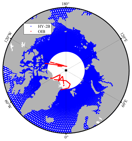
Figure 1Ground tracks of the HY-2B SGDR product (blue points) and flight tracks of Operation IceBridge (OIB) airborne experiments (red points) across the Arctic in April 2019.
2.2 CryoSat-2 radar altimeter
CS-2 was launched by the ESA in April 2010 with an orbital altitude of approximately 717 km, an orbital inclination of 92∘ and a repeat cycle period of 369 d. It has a 30 d subcycle and can realize monthly observations of the Arctic with a coverage of 88∘ N/S. CS-2 carries a Ku-band SAR Interferometric Radar Altimeter (SIRAL) that can obtain the surface elevations of ground objects. This SIRAL uses delayed Doppler radar altimeter technology to reduce the satellite observation footprint to approximately 0.3 km along the track and 1.5 km across the track.
Currently, there are five main kinds of CS-2 sea ice thickness products: those from the ESA, the Centre for Polar Observation and Modelling (CPOM) (Laxon et al., 2003; Tilling et al., 2017), the AWI (Ricker et al., 2014; Hendricks and Ricker, 2020), the National Snow and Ice Data Center (NSIDC) (Kurtz et al., 2014; Kurtz and Harbeck, 2017), and the ESA Climate Change Initiative (CCI) (Paul et al., 2017). These products are constructed using different retrack algorithms. Furthermore, the upcoming releases of CryoTEMPO are expected to be a favourable product to be used in the future by the scientific community. We mainly used level-2 (L2) along-track data published by the ESA (processor baseline-D) and monthly average products published by the AWI.
2.3 ICESat-2 laser altimeter
The Advanced Topographic Laser Altimeter System (ATLAS) aboard IS-2 is a low-pulse energy laser (operating wavelength: 532 nm) that uses photon-counting technology to emit pulses at a repetition rate of 10 kHz (Degnan, 2002). The photon detector accurately calculates the round-trip time of these photons from the satellite to the ground and back to obtain distance measurements. We used the snow freeboard data of ATL20 products in the study (version 003, Petty et al., 2021); these products were provided by the National Aeronautics and Space Administration (NASA). The ATL20 snow freeboard was calculated by subtracting the local sea surface height (SSH) from the sea ice elevation. The average value of the specular reflected elevation of the inter-ice channel collected in the 10 km segment where the measurement point was located was used as the SSH estimation value (Kwok et al., 2021). The 10 km segments were selected to minimize the impact of the sea surface slope on the sea ice freeboard height estimations, as SSHs are generally constant within 10 km segments in polar regions north of 60∘ N. If SSH data were not available within a segment, the total freeboard estimate was not provided, thus assuring the reliability of the total freeboard estimates. Finally, the total freeboard height was gridded into a 25 km spatial grid, and the average value of the total freeboard height of all observation points in the grid was used as the total freeboard height of that grid. Assuming hydrostatic equilibrium, we used IS-2 snow freeboard products to calculate sea ice thicknesses with AWI snow depth products and compared them with HY-2B and CS-2.
2.4 OIB airborne data
The airborne OIB experiment is an aerial remote sensing polar-region observation project started by NASA in 2009. Its initial purpose is to compensate for the data gaps that arise during the operation of ICESat and IS-2 satellites and to carry out large-scale sea ice detection experiments in the Arctic from March to May and in the Antarctic from October to November every year. Figure 1 shows the flight path of the OIB in the Arctic in April 2019. In this study, we used IceBridge level-4 data (IDCSI4) to evaluate the sea ice freeboard and sea ice thickness retrieved by HY-2B and CS-2. In addition, we gridded the OIB data to a 25 km polar stereographic grid and set no fewer than 100 observation points inside each grid to optimally solve the limited representation problem of the OIB data.
2.5 Auxiliary data
We used auxiliary data, including sea ice concentration (SIC), sea ice type, mean sea surface (MSS) height, snow depth, and snow density, in this study. The SIC (version OSI-401-b) and sea ice type (version OSI-403-b) data were released by the European Organization for Meteorological Satellites (EUMETSAT) Ocean and Sea Ice Satellite Application Facility (OSI-SAF). The MSS data were released by the Technical University of Denmark (DTU).
2.5.1 Sea ice concentration
Tonboe et al. (2016) used the brightness temperatures of the 19-V, 37-V and 37-H channels in the Special Sensor Microwave Imager/Sounder (SSMIS) scanning radiometer to retrieve SICs with a hybrid algorithm constructed from the Bristol algorithm and bootstrap algorithm. To ensure optimum performances over both marginal and consolidated ice and to retain the virtues of each algorithm, the Bristol algorithm is given low weights at low concentrations, while the opposite is the case for high-ice-concentration regions (Tonboe et al., 2016). The SIC data are provided as a daily average grid product with the 10 km Lambert azimuthal grid. We used these SIC data to screen the altimeter data, and altimeter observations corresponding to areas with SICs greater than 70 % were used in the sea ice freeboard calculations.
2.5.2 Sea ice type
We used sea ice type data to distinguish first-year ice (FYI) from multiyear ice (MYI). Aaboe et al. (2021) used the gradient ratio (GR) of in Advanced Microwave Scanning Radiometer 2 (AMSR-2) microwave radiometer data and the scattering coefficient in Advanced Scatterometer (ASCAT) microwave data to calculate the ice type probability. The sea ice type data are provided as a daily average grid product with a 10 km Lambert azimuthal grid.
2.5.3 MSS height
In this study, we employed the DTU18 MSS model to eliminate errors due to unresolved gravity features, inter-satellite biases and remaining satellite orbit errors. After subtracting the MSS, we are able to precisely determine the instantaneous elevation of lead (Skourup et al., 2017). The DTU18 MSS model is fused with the data of several satellite altimeters, such as TOPEX/Poseidon (T/P), Jason-1 (J1), Jason-2 (J2), ERS-1, ERS-2, ENVISAT, ICESat, Geosat, Geosat Follow-On (GFO) and CryoSat-2 (Andersen et al., 2018a, b).
2.5.4 Snow depth
Hendricks and Ricker (2020) obtained a composite snow depth product (hereafter referred to as the AWI snow depth product) by fusing climatology snow depths from Warren et al. (1999, hereinafter W99) with the daily average AMSR-2 snow depths of the University of Bremen. To merge these two datasets, the authors created a monthly average AMSR-2 snow depth product to match the W99 climatology snow depths from October to April. They then low-pass filtered the monthly average AMSR-2 snow depths with a Gaussian filter with a size of eight grid cells, removed negative snow depth values and limited the upper range to 60 cm. Finally, they created a regional weighting factor to ensure a smooth transition between the two types of data in the borderline area. Since the W99 climatology snow depths on FYI are higher, they had to be corrected by a coefficient of 0.5 (Kwok and Cunningham, 2015). However, the AMSR-2 snow depths on FYI did not need to be modified, so the authors introduced a total scaling factor to correct the contribution of W99 (Hendricks and Ricker, 2020). The AWI snow depth products are provided as monthly averaged grid products using the Equal Area Scalable Earth Grid version 2 (EASE-2) for the Northern Hemisphere with a spatial resolution of 25 km.
2.5.5 Snow density
To minimize differences in sea ice thicknesses at the beginning of the sea ice growing season, we used the evolving snow density values proposed by Mallett et al. (2020). These values are consistent with the snow densities used in the AWI CS-2 sea ice thickness product. The density equation of snow is shown in Eq. (1).
where t represents the number of months since October.
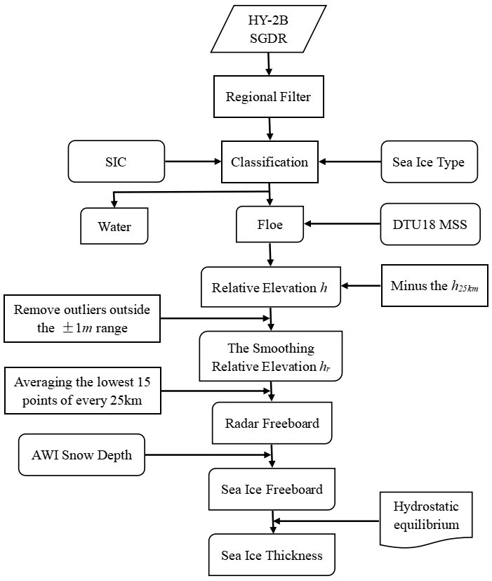
In this section, we describe the sea ice thickness retrieval method applied for the SGDR data of the HY-2B pulse-limited radar altimeter in detail. The technical process of retrieving sea ice thickness based on HY-2B SGDR data is shown in Fig. 2. The specific retrieval process is as follows:
-
NaN (not a number) values in the SGDR data and data south of 60∘ N were eliminated. Due to the influence of instrument noise, atmospheric factors and tidal factors during the propagation of pulse signals, it was necessary to consider the dry and wet tropospheric delay correction (National Centers for Environmental Prediction, NCEP), inverse barometric correction (NCEP), ionospheric correction (GIM), ocean tidal correction (Goddard Space Flight Center, GSFC, GOT4.10c), ocean load tidal correction (GSFC, GOT4.10c), earth tidal correction (Cartwright and Edden, 1973) and polar tidal correction (Wahr, 1985) when calculating the surface elevation (Zhang et al., 2022).
-
The SICs of data points in all HY-2B orbits were obtained using nearest interpolation. We used altimeter observations to calculate the radar freeboard for areas with SIC greater than 70 %. Sea ice was classified into FYI, MYI, and ambiguous ice using sea ice type data, and ambiguous ice was not considered for the subsequent sea ice thickness retrievals.
-
The MSS height product DTU18 (Andersen et al., 2018a, b) was subtracted from the geolocated surface elevations to remove geoid fluctuations, that is, the derived relative elevations of ground objects h (Ollivier et al., 2012; Zhang et al., 2021). The estimation error does not include the modelled portion of the sea surface height but includes all the unexplained static and time-varying components of the sea surface as well as noise introduced by our estimation process, including the errors of orbit determination and different tracking algorithms (Kwok et al., 2007). The estimation error of sea surface height was eliminated by subtracting the average value of every 25 km (h25 km) along the track (Kwok et al., 2007; Zhang et al., 2021), as shown in Eq. (2). In addition, the relative surface elevations, hr, outside the range +1.0 to −1.0 m are removed from processing, as shown in Fig. 3a and b. Equation (2) can be expressed as follows:
where hr is the relative surface elevation after eliminating residuals (unit: m), h is the relative elevation of ground objects (unit: m) and h25 km is the average value every 25 km (unit: m).
-
If more than or equal to 15 observation points were available per 25 km in the track data, the average of the 15 lowest values was taken as the SSHA. Otherwise, the SSHA was considered to be NaN, and nearest interpolation was performed along the track. The SSHA was subtracted from the observed values hr inside each 25 km segment to obtain the radar freeboard height, as shown in Eq. (3) and Fig. 3b and c. Since the HY-2B SGDR product has been retracked for the Brown model (Zhang et al., 2022), we are simply using the range terms from the satellite to the ground already provided in the SGDR product. Equation (3) can be expressed as follows:
where fr is the radar freeboard (unit: m), hr is the relative surface elevation after eliminating the residual (unit: m) and SSHA is the sea surface height anomaly (unit: m).
-
Due to the attenuation of electromagnetic waves when they pass through snowpack, it is necessary to correct the radar freeboard based on the AWI snow depth, as shown in Eq. (4) (Hendricks and Ricker, 2020; Glissenaar et al., 2021). Several studies have found that radar freeboard uncertainty also pertains to inconsistent knowledge on how far the radar signal penetrates into the overlying snow cover (Nandan et al., 2020; Willatt et al., 2011, 2010; Drinkwater et al., 1995). The general assumption is that the radar return primarily originates from the snow–sea-ice interface at the Ku band. While this may be applicable to cold, dry snow in a laboratory (Beaven et al., 1995), scientific evidence from observations and modelling indicates that this assumption may not be valid even for a cold, homogeneous snowpack (Nab et al., 2023; Nandan et al., 2020; Willatt et al., 2011, 2010; Tonboe et al., 2010). Moreover, field campaigns have revealed that dominant radar scattering actually occurs within the snowpack or at the snow surface rather than at the snow–ice interface (Stroeve et al., 2020; Willatt et al., 2011, 2010; Giles et al., 2007). Since we do not currently have methods that can take into account this change in the scattering horizon within the snowpack, we have assumed that the radar pulses penetrate through any snow cover on ice floes and scatter from the snow–ice interface.
where f is the sea ice freeboard (unit: m), fr is the radar freeboard (unit: m), hs is the AWI snow depth (unit: m), c is the speed of light in vacuum and cs is the speed of light through snow, parameterized by Eq. (5) (Ulaby et al., 1986).
where ρs is the snow density (Mallett et al., 2020).
-
The sea ice freeboard data were converted to sea ice thickness data by assuming hydrostatic equilibrium, as shown in Eq. (6). To obtain monthly grid values, we averaged all thickness measurements within a 25 km radius of the centre of each grid cell, with all points receiving equal weighting:
where T is the sea ice thickness (unit: m), ρw is the water density and ρi is the sea ice density. We used a fixed FYI density estimate of 916.7 kg m−3 and an MYI density estimate of 882 kg m−3 (Alexandrov et al., 2010).
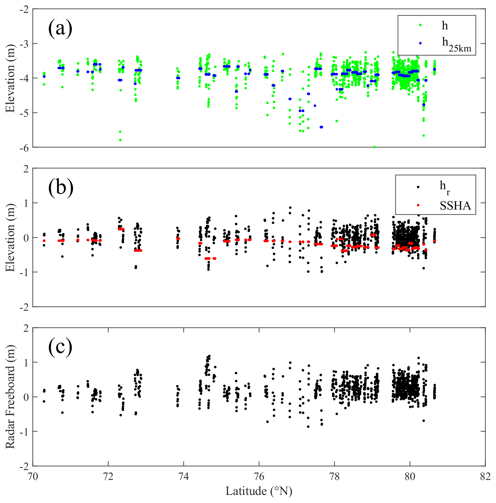
Figure 3A sample of the HY-2B elevation profile obtained for track number 14418 on 4 April 2020. The green points in panel (a) are the relative elevation (h) values; the blue points in panel (a) are the h25 km values, defined as the 25 km running mean of h; the black points in panel (b) are the modified relative elevation (hr) values; the red points in panel (b) are the sea surface height anomaly (SSHA) values; and the black points in panel (c) are the radar freeboard values.
In this section, we used the method proposed in Sect. 3 to retrieve the HY-2B radar freeboard and sea ice thickness during the two periods of interest (from October 2019 to April 2020 and from October 2020 to April 2021). First, we compared the parameters involved in the retrieval process with those in the CS-2 L2 along-track data released by the ESA. Second, we also compared the results with the CS-2 radar freeboard and sea ice thickness released by the AWI during the same periods and analysed the differences between the HY-2B and CS-2 products with regard to different sea ice types. Finally, we used airborne and satellite laser altimetry as a reference.
4.1 Comparison of along-track freeboard estimates
The orbit settings for HY-2B and CS-2 are different in that it is impossible to compare their radar freeboard estimates from the same position at the same time, so we compare the radar freeboard estimates of HY-2B and CS-2 on adjacent tracks within the Beaufort Sea, as shown in Fig. 4. Table 2 summarizes the mean and standard deviation values of the relative surface elevation, SSHA, and radar freeboard estimates based on HY-2B and CS-2. We selected two instances of different time for comparison acquired on 4 April 2020 and 13 March 2020, respectively, as shown in Fig. 4a and e. For each date we denote the time of CS-2 and HY-2B tracks. Both of them cover the Beaufort Sea and the northern Canadian Arctic Archipelago. In addition, both orbits cover the FYI (grey) and MYI (black) regions. Figure 4b, c, f and g show that the mean relative surface elevations of HY-2B/CS-2 in these two periods are 0 m/0 m and 0.081 m/0.087 m, respectively. We find that the relative surface elevations of HY-2B are slightly lower than those of CS-2, which may have been caused by the fact that not all points used to estimate the SSHA within the 25 km segments originate from leads. The mean SSHAs of HY-2B/CS-2 in the two periods are −0.21 m/−0.11 m and −0.051 m/−0.069 m, respectively. We find that the SSHAs estimated by HY-2B are lower than those estimated by CS-2, and the SSHA dispersions estimated by HY-2B are larger than those estimated by CS-2. These differences may be caused by the error of orbit determination, different tracking algorithms and different derivation methods of SSHA. Figure 4d and h show the radar freeboard estimates of HY-2B and CS-2 in the two periods, respectively. We find that the radar freeboard estimates of HY-2B are larger than those of CS-2. The anomalous radar freeboards are directly related to the SSHAs and the relative surface elevation of the ice floes. In addition, the selected tracks from HY-2B and CS-2 are not fully coincident; hence, freeboard differences are also induced by the location and time period differences between the two products.
Table 2Comparison of the mean and standard deviation values of the relative surface elevation (hr), sea surface height anomaly (SSHA) and radar freeboard estimates (fr) from HY-2B and CryoSat-2.
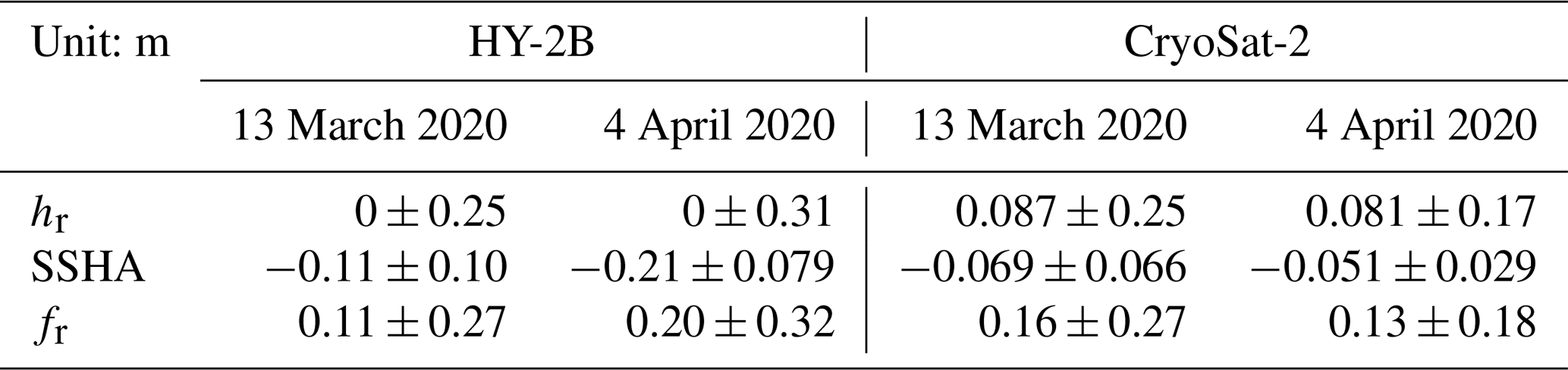
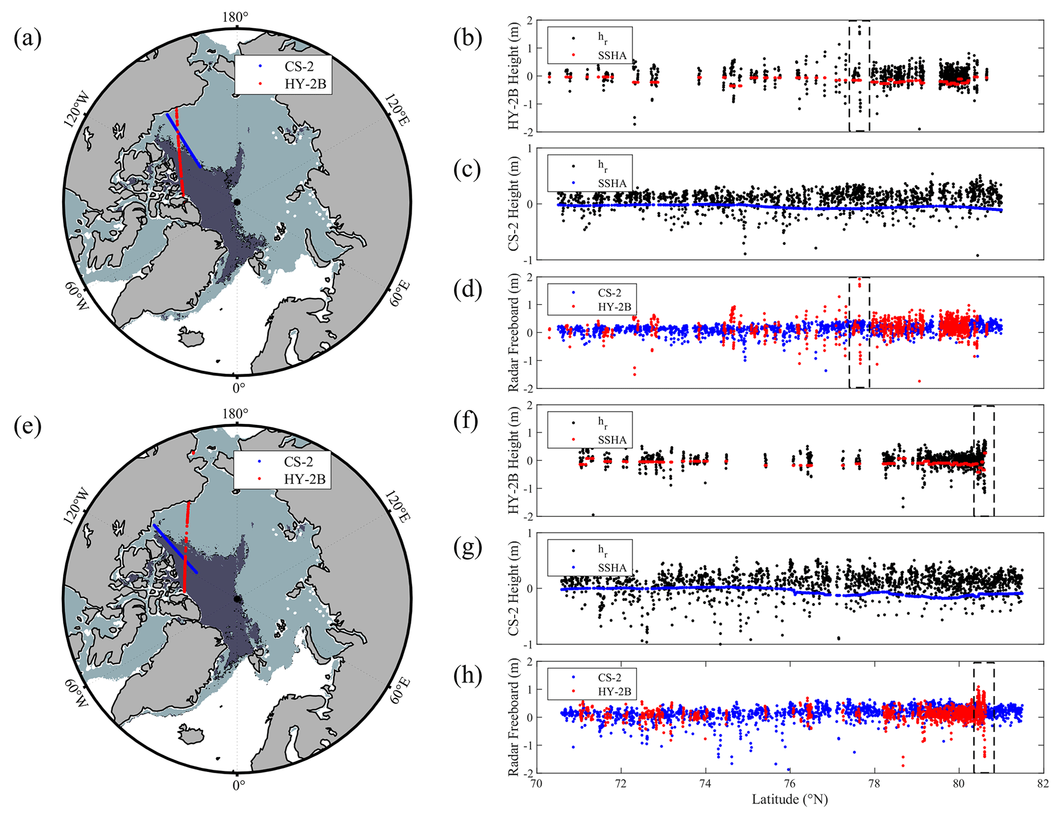
Figure 4(a, e) CryoSat-2 (blue) and HY-2B (red) tracks (acquired on 4 April and 13 March 2020, respectively) selected for comparison. FYI regions: light shading; MYI regions: dark grey shading. (b, f) HY-2B relative surface elevations of floes (black dots) and SSHAs (red dots) corresponding to the tracks shown in panels (a) and (e), respectively. (c, g) CryoSat-2 relative surface elevations of floes (black dots) and SSHAs (red dots) corresponding to the tracks shown in panels (a) and (e), respectively. (d, h) CryoSat-2 (blue) and HY-2B (red) radar freeboard values corresponding to the tracks shown in panels (a) and (e), respectively.
4.2 Comparison with AWI CS-2 radar freeboard data
Based on the HY-2B SGDR data, we analyse the HY-2B monthly average radar freeboard data collected from October 2019 to April 2020 while also comparing them with the AWI CS-2 radar freeboard recorded during the same period, as shown in Fig. 5. The spatial patterns of the HY-2B and CS-2 data are in broad agreement; that is, thicker radar freeboards occur north of the Canadian Arctic Archipelago, while thinner radar freeboards occur in other seas. Since the height of the lead is usually lower than the height of the adjacent floes, our method is reasonable where there are more leads in the 25 km segment. Despite this good spatial consistency, the HY-2B radar freeboards are generally thicker than those of AWI CS-2, except in spring (March and April). In spring, more of the lowest 15 points within the 25 km segment are likely to originate from floes, while in early winter, more points may originate from leads. Therefore, the radar freeboards in spring are lower than those of CS-2. The mean deviations of the radar freeboard between HY-2B and AWI CS-2 range from −0.035 to 0.016 m from October 2019 to April 2020. The HY-2B radar freeboards are generally higher than those of AWI CS-2 in the FYI region and lower than those of AWI CS-2 in the MYI region. More of the lowest 15 points within the 25 km segment are likely to originate from floes in the MYI region, and more points may originate from leads in the FYI region. Therefore, the radar freeboard in the MYI region is lower than that of CS-2. The HY-2B spatial coverage is limited to 81∘ N/S, while the CS-2 coverage is limited to 88∘ N/S, so the monthly average radar freeboard of HY-2B retrievals lacks observation data in the Arctic central region. Therefore, the HY-2B radar freeboard results are sparse in early winter (October to December 2019).
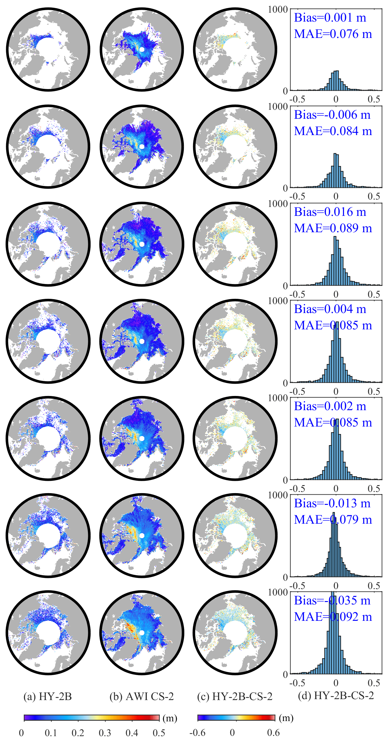
Figure 5Comparisons and differences between the HY-2B radar freeboard and AWI CS-2 radar freeboard recorded from October 2019 to April 2020: (a) HY-2B radar freeboards, (b) CS-2 radar freeboards, (c) spatial differences between HY-2B and CS-2 radar freeboards, and (d) a histogram of differences between HY-2B and CS-2 radar freeboards.
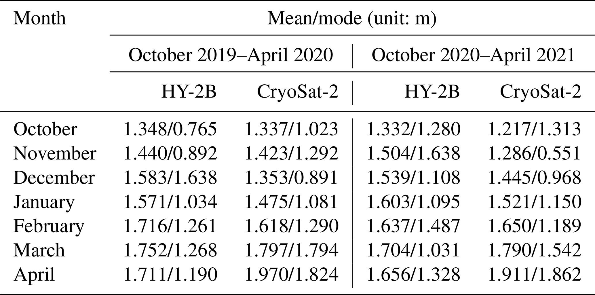
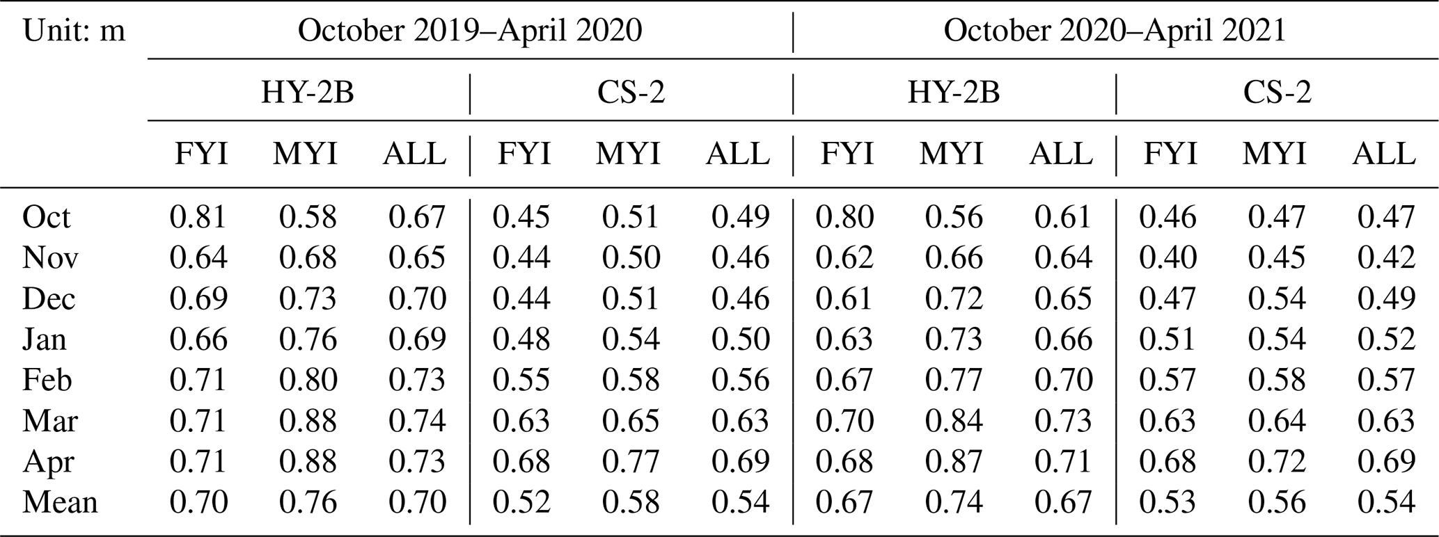
Table 3 shows the mean and modal radar freeboards of HY-2B and AWI CS-2 from October 2019 to April 2020 and from October 2020 to April 2021. For comparison, only the overlapping data points in the two satellite products are considered. The AWI CS-2 mean freeboards are larger than the CS-2 modal freeboards in all months (Schwegmann et al., 2016). The HY-2B mean freeboards are also thicker than the HY-2B modal freeboards in all months. However, despite the similarities between the two satellite products, there are also clear differences between them. The mean freeboard differences and modal freeboard differences in spring between HY-2B and CS-2 are both larger than those in early winter. Table 3 also indicates that the spring radar freeboard retrieved by our method is lower than that of CS-2. Moreover, the HY-2B radar freeboard has a smaller linear growth rate than CS-2, which is also reflected in Fig. 7a.
Table 3Mean and modal radar freeboard values of HY-2B and CryoSat-2 over the common area.
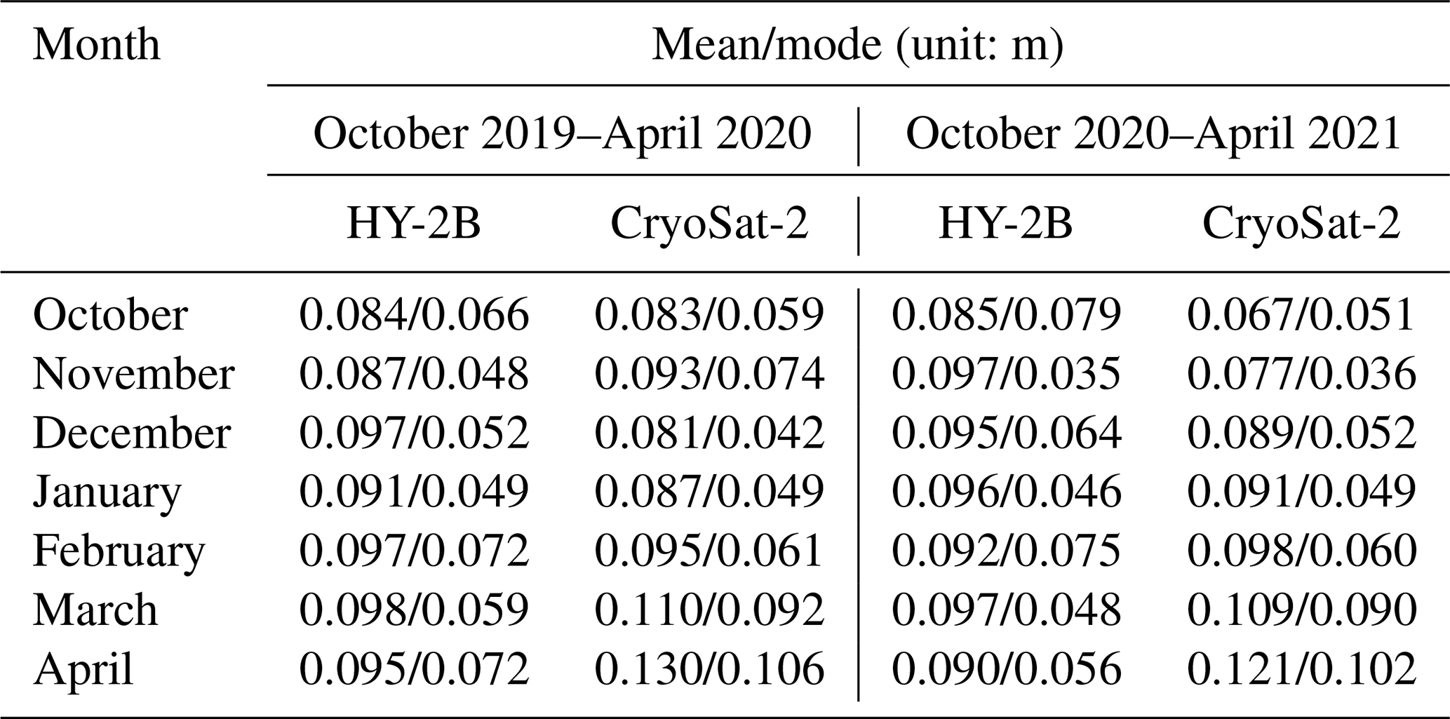
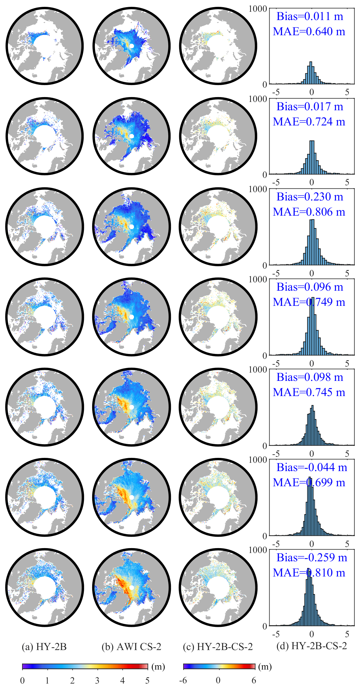
Figure 6Comparisons and differences between HY-2B sea ice thickness and AWI CS-2 sea ice thickness from October 2019 to April 2020, (a) HY-2B sea ice thicknesses, (b) CS-2 sea ice thicknesses, (c) spatial differences between HY-2B and CS-2 sea ice thicknesses, and (d) a histogram of the differences between HY-2B and CS-2 sea ice thicknesses.
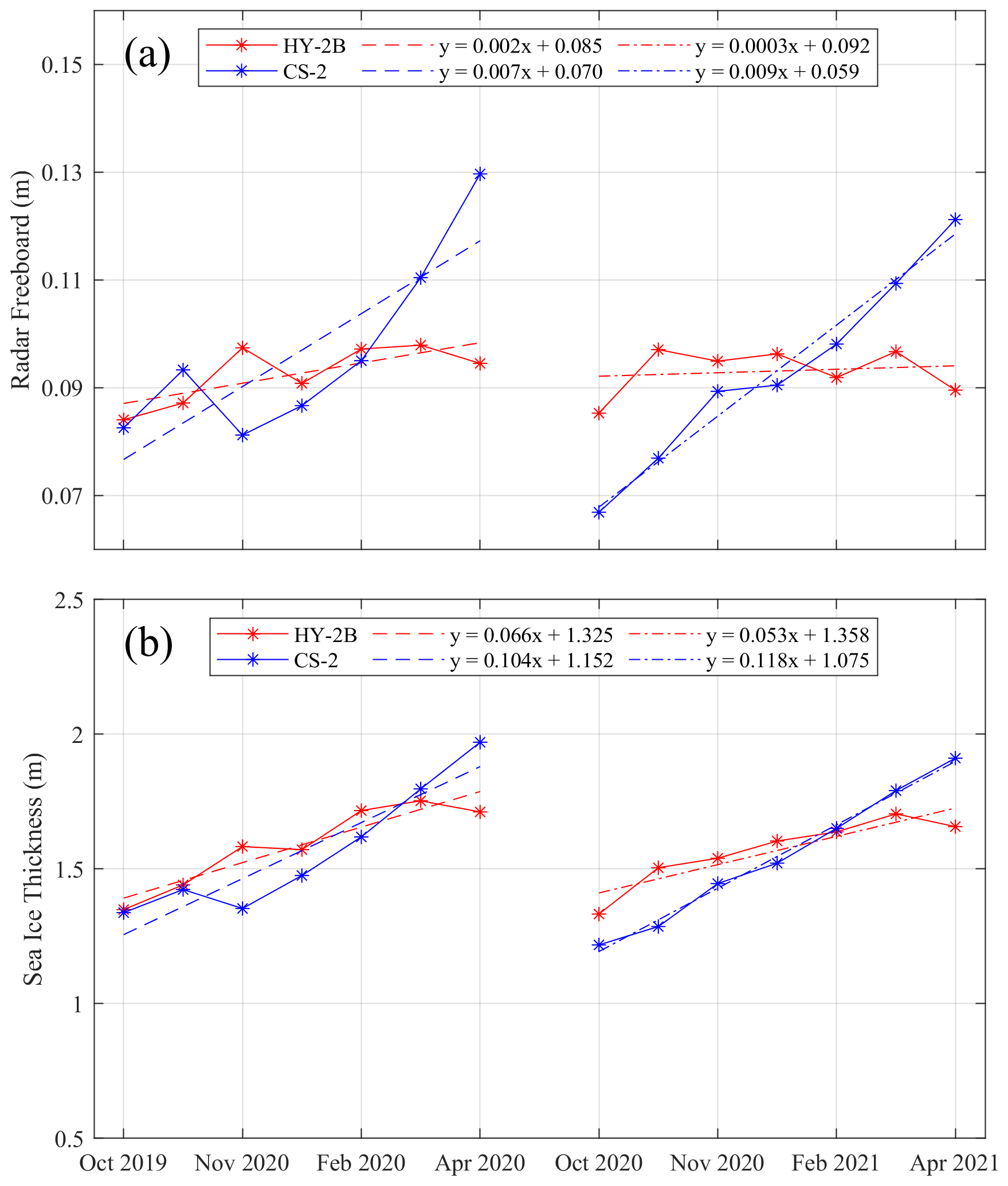
Figure 7Seasonal variation trends of HY-2B and CryoSat-2 radar freeboard and sea ice thickness from October 2019 to April 2020 and from October 2020 to April 2021. (a) Radar freeboard and (b) sea ice thickness; HY-2B: red, CS-2: blue.
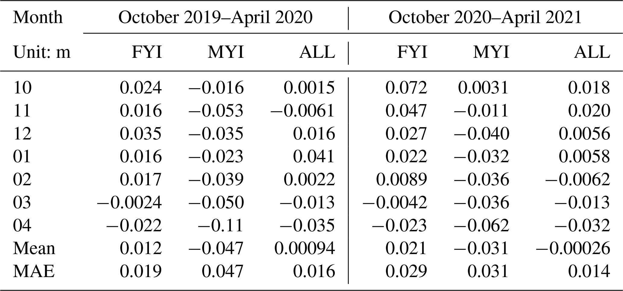
To assess the deviations between the HY-2B and AWI CS-2 radar freeboards on various sea ice types, we list the differences in FYI, MYI and total sea ice between the two satellite products in Table 4. The radar freeboard deviation between HY-2B and AWI CS-2 over MYI is larger than that over FYI, with deviations of approximately 3 cm on FYI (positive) and 5 cm on MYI (negative). In addition, the mean deviations of the radar freeboard between HY-2B and AWI CS-2 change from positive to negative over time. In March and April, the deviations between HY-2B and AWI CS-2 are negative for FYI, MYI and total sea ice, indicating that the HY-2B radar freeboards are smaller than those of AWI CS-2. In general, the HY-2B radar freeboards exhibit a mean absolute error (MAE) of approximately 0.02 m with respect to CS-2 (Table 4). We think that the MAEs may have been caused by the error of orbit determination, retracking algorithm and the accuracy of the extracted HY-2B SSHAs.
Table 4Differences in the monthly mean radar freeboard values of HY-2B and CryoSat-2 on FYI, MYI and total sea ice.
4.3 Comparison of sea ice thickness with AWI CS-2 data
Figure 6 shows the spatial comparison of Arctic SIT between HY-2B and AWI CS-2 from October 2019 to April 2020. The spatial patterns of the two sea ice thickness products exhibited broad agreement; thicker sea ice occurred north of the Canadian Arctic Archipelago, while thinner sea ice occurred in the Eurasian continental marginal sea and Baffin Bay. Both products show similar seasonal changes in which the Arctic sea ice thickness gradually thickens. Although the spatial distributions are consistent, the HY-2B sea ice thicknesses are thicker than those of CS-2, except in spring (March and April). This is mainly due to the thicker HY-2B radar freeboards than those of CS-2. The mean deviations in sea ice thickness between HY-2B and AWI CS-2 range from −0.259 to 0.230 m from October 2019 to April 2020. Due to the lower radar freeboards in spring than those of CS-2, the sea ice thicknesses are also lower in spring than those of CS-2. The HY-2B sea ice thicknesses are generally higher than those of AWI CS-2 in the FYI region and lower than those of AWI CS-2 in the MYI region. In all months, the MAEs of sea ice thickness between HY-2B and AWI CS-2 are within 0.9 m. The HY-2B sea ice thickness has a smaller linear growth rate than CS-2, which is also reflected in Fig. 7b.
Table 5 lists monthly mean and modal sea ice thickness values derived from HY-2B and AWI CS-2 from October 2019 to April 2020 and from October 2020 to April 2021. For comparison, only the overlapping data points in the two satellite products are considered. The AWI CS-2 mean thicknesses are larger than the modal thicknesses in all months. The HY-2B mean thicknesses are also thicker than the modal thicknesses, except in December 2019 and November 2020. Because the distribution of the HY-2B sea ice thickness is close to a Gaussian distribution, the modal may be close to the mean or even slightly greater than the mean. The monthly mean sea ice thicknesses of HY-2B are thicker than those of CS-2 in early winter, while the CS-2 sea ice thicknesses are greater than those of HY-2B in spring. The modal thicknesses of HY-2B are thinner than those of AWI CS-2, except in December 2019, November 2020 and December 2020. These results are related to the accuracy of the extracted HY-2B SSHAs.
Table 5Mean and modal sea ice thickness values of HY-2B and CryoSat-2 in the common area.
To assess the deviations between the HY-2B and AWI CS-2 sea ice thicknesses among various sea ice types, we list the deviations in FYI, MYI, and total sea ice, as listed in Table 6. On FYI, the HY-2B sea ice thicknesses are thicker than those of AWI CS-2, except in March and April. In MYI, the HY-2B sea ice thicknesses are thinner than those of AWI CS-2 in all months. In addition, the mean deviations in sea ice thickness between HY-2B and AWI CS-2 change from positive to negative over time. In general, the HY-2B sea ice thicknesses exhibit an MAE of approximately 0.2 m with respect to CS-2 (Table 6). The MAEs are directly affected by the accuracy of the retrieved radar freeboard values.
Table 6Differences in the monthly mean sea ice thicknesses of HY-2B and CryoSat-2 on FYI, MYI and total sea ice.
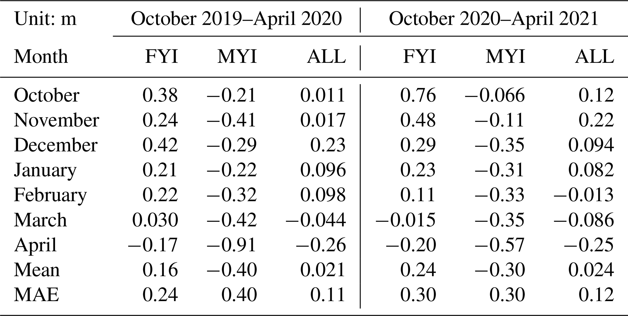
Figure 7 shows the seasonal variation trends of the HY-2B and AWI CS-2 radar freeboards and sea ice thicknesses during two sea ice growing cycles averaged over the overlapping regions. We calculate the average radar freeboard and sea ice thickness over the common area. The growth trend of the HY-2B radar freeboards is slower than that of the AWI CS-2. As shown in Fig. 7a, the HY-2B radar freeboards are higher than the AWI CS-2 in winter, while the opposite pattern is observed in spring. The seasonal trend of sea ice thickness is also similar to that of the radar freeboard. The growth rate of AWI CS-2 sea ice thickness is approximately twice that of HY-2B, as shown in Fig. 7b.
4.4 Comparison with OIB and IS-2 data
We use the HY-2B SGDR data collected in April 2019 to retrieve sea ice freeboard and sea ice thickness and compare the OIB airborne observations with HY-2B and AWI CS-2, as shown in Fig. 8. Because the HY-2B radar altimeter can cover only the 81∘ N/S region, only 13 grids could be evaluated when overlapped with the OIB airborne data collected in the same period. The correlation between the HY-2B sea ice freeboard and OIB is 0.77, with a root mean square error (RMSE) of 0.13 m and an MAE of 0.12 m. The correlation between the AWI CS-2 sea ice freeboard and OIB is 0.84, with an RMSE of 0.10 m and an MAE of 0.081 m. Based on hydrostatic equilibrium, we use the AWI snow depth data to convert sea ice freeboard into sea ice thickness, which is verified against OIB sea ice thickness, as shown in Fig. 8c and d. The correlation between HY-2B and OIB is 0.65, with an RMSE of 1.86 m and an MAE of 1.72 m, suggesting that this underestimation of sea ice thickness could be attributed not only to sea ice freeboard but also to snow depth or other parameters. The correlation between AWI CS-2 sea ice thickness and OIB is 0.80, with an RMSE of 1.00 m and an MAE of 0.75 m. The majority of the spread (shown by RMSE or MAE) in our HY-2B evaluation is caused by the underestimation of thickness over thick ice, which may have been caused by the fact that not all points used to estimate the SSHA within the 25 km segments originate from leads.
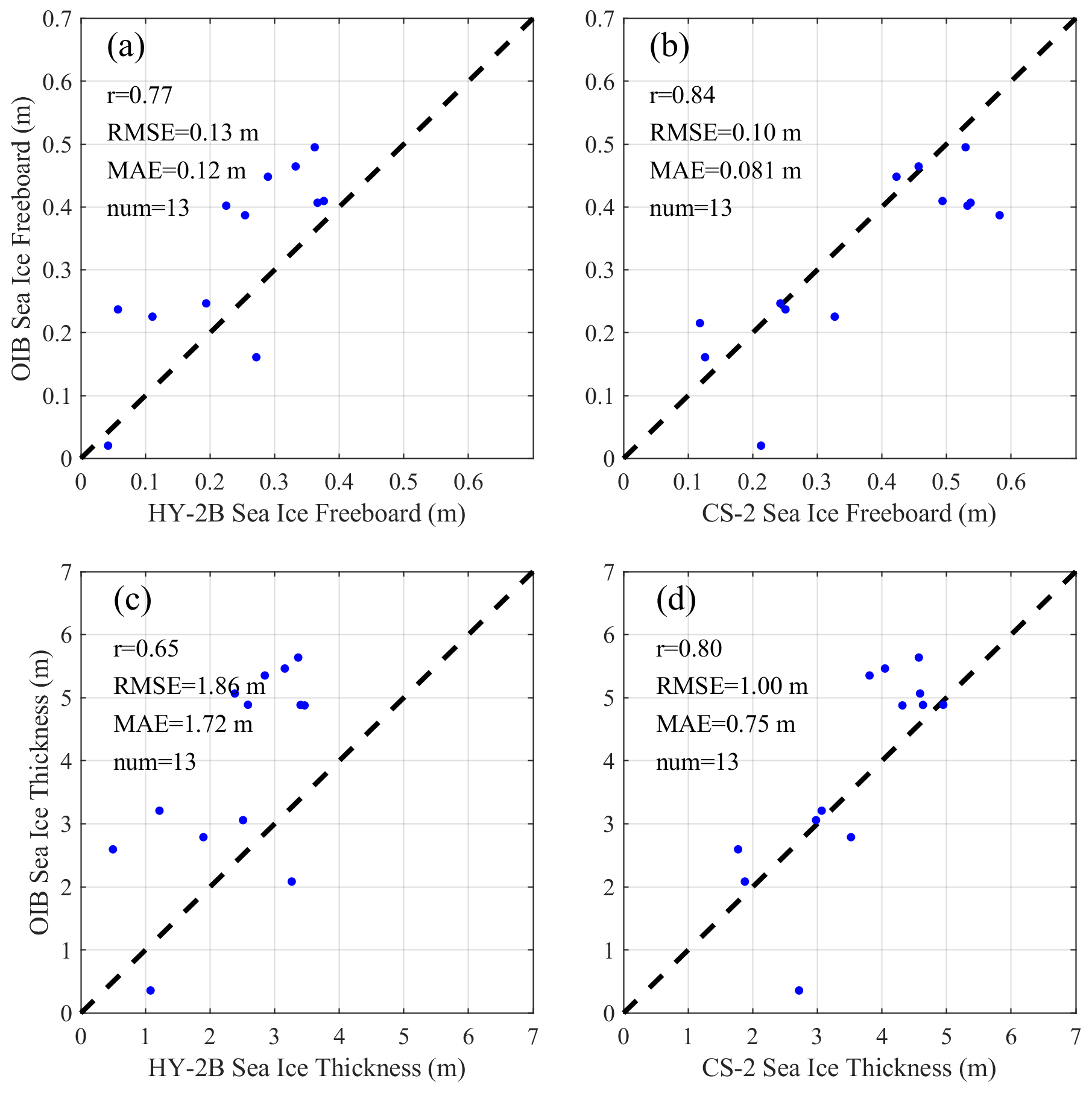
Figure 8Comparative scatter plots between two satellite products and OIB collected in April 2019: (a) HY-2B sea ice freeboard vs. OIB sea ice freeboard, (b) AWI CS-2 sea ice freeboard vs. OIB sea ice freeboard, (c) HY-2B sea ice thickness vs. OIB sea ice thickness and (d) AWI CS-2 sea ice thickness vs. OIB sea ice thickness.
IS-2 laser altimeters have a range that reaches the snow surface on sea ice and therefore are not impacted by the uncertain scattering horizons within snow layers (Magruder et al., 2020). The spatial resolutions (approximately 11 m of the measurement footprint, Fons et al., 2021) of these altimeters are much higher than those of CS-2 (approximately 0.3 km along the track and 1.5 km across the track) and HY-2B (approximately 1.9 km across the track), thus providing independent all-Arctic snow freeboard data that can be compared with the HY-2B and CS-2 retrievals. The AWI snow depths are subtracted from the IS-2 snow freeboards to obtain the sea ice freeboards. To compare these values with the IS-2 sea ice freeboard, we use the AWI snow depth to perform a wave propagation speed correction for the HY-2B and AWI CS-2 radar freeboards (see Sect. 3). Figure 9 shows monthly comparisons of sea ice freeboard between HY-2B and IS-2 and between CS-2 and IS-2 from October 2019 to April 2020 and from October 2020 to April 2021, respectively. The RMSEs obtained between HY-2B and IS-2 range from 0.13 to 0.16 m, and the MAEs range from 0.09 to 0.12 m. The RMSEs between CS-2 and IS-2 range from 0.09 to 0.12 m, and the MAEs range from 0.07 m to 0.10 m. We observe that HY-2B generates a significantly thicker sea ice freeboard than IS-2. The abnormal values from HY-2B may be caused by the error of orbit determination, the tracking algorithm of the Brown model and the determination algorithm of SSHA. In addition, the differences between HY-2B and IS-2 may be caused by inconsistent measurement modes and footprint sizes.
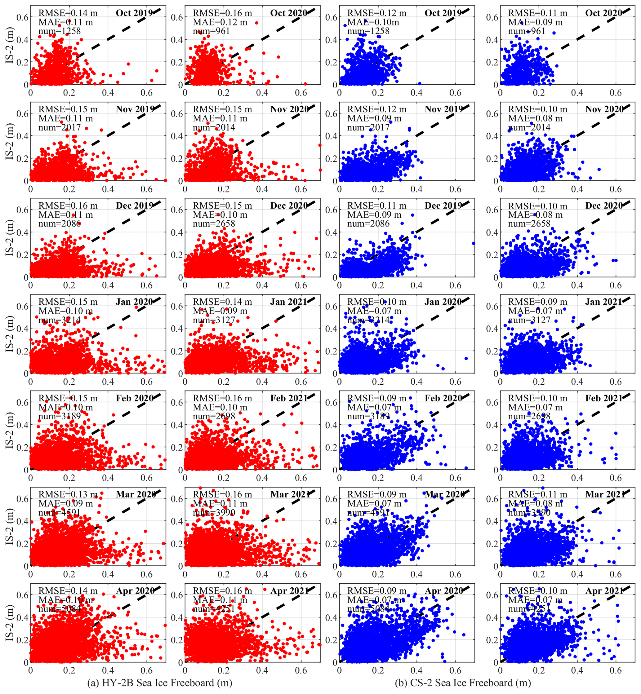
Figure 9Monthly comparisons between HY-2B sea ice freeboard and ICESat-2 sea ice freeboard and between CryoSat-2 sea ice freeboard and ICESat-2 sea ice freeboard values: panel (a) shows comparisons between HY-2B and ICESat-2 in red points, and panel (b) shows comparisons between CS-2 and ICESat-2 in blue points.
Assuming hydrostatic equilibrium, HY-2B and CS-2 sea ice freeboards are converted to sea ice thicknesses using AWI snow depth, and the results are compared with IS-2 sea ice thicknesses. Figure 10 shows comparisons of the HY-2B and CS-2 sea ice thicknesses with IS-2. The RMSEs of sea ice thickness derived between HY-2B and IS-2 range from 1.21 to 1.48 m, and the MAEs range from 0.79 to 1.00 m. The RMSEs derived between CS-2 and IS-2 range from 0.77 to 0.93 m, and the MAEs range from 0.56 to 0.74 m. The RMSE and MAE of sea ice thickness are thus related not only to sea ice freeboard and snow depth but also to sea ice type and snow density (Ricker et al., 2014).
In this section, we first compared the effects of the SSHAs extracted under different parameter schemes on the HY-2B radar freeboard retrievals. We then discussed the uncertainties of the HY-2B sea ice freeboard and sea ice thickness.
5.1 Influence of different SSHA determination schemes on the HY-2B radar freeboard
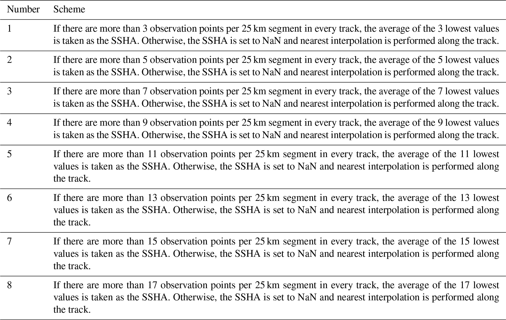
Ricker et al. (2014) believed that the random uncertainty of the radar freeboard can be determined by the speckle noise and actual accuracy of SSHAs. Therefore, it is crucial to accurately extract SSHAs in the HY-2B radar freeboard retrievals in this work. We adopt eight schemes to determine these SSHAs and apply them to retrieve the HY-2B radar freeboard. The specific parameter schemes are listed in Table 7. Moreover, the HY-2B radar freeboard retrievals are compared to the AWI CS-2 radar freeboard collected during the same period. The mean deviation, MAE and SSHA values retrieved between the two satellites under different schemes from October 2019 to April 2020 and from October 2020 to April 2021 are listed in Table 8. As the table shows (schemes 1–8), the mean deviation and MAE values first decrease and then increase with the gradual increase in SSHA, indicating that an increase in SSHA does not necessitate a linear reduction in mean deviation or MAE. The SSHA values of Scheme 8 are the largest; both are greater than −0.1 m. The mean deviations of gridded radar freeboard between HY-2B and CS-2 are all less than 0, indicating that the HY-2B radar freeboard retrievals are generally lower than the AWI CS-2 radar freeboards. In addition, the MAE of Scheme 8 is larger than that obtained under Scheme 7. Finally, according to the mean deviation and MAE values, we use Scheme 7 to extract SSHAs to retrieve the HY-2B radar freeboards. The cumulative probability of measuring points greater than or equal to 15 within each 25 km segment is 43.4 %. It is worth noting that the HY-2B radar freeboard and sea ice thickness retrieved by Scheme 7 result in slower growth rates compared to CS-2. In spring, more of the lowest 15 points within the 25 km segment are likely to originate from floes, while more points may originate from leads in early winter. As a result, the errors of the retrieved HY-2B radar freeboard and sea ice thickness are smaller in winter than in spring. Therefore, the HY-2B sea ice freeboard and sea ice thickness values are lower than those of CS-2 in spring, especially in March and April, as shown in Tables 3 and 5.
5.2 Uncertainty of HY-2B sea ice freeboard and sea ice thickness data
The speckle noise caused by instrument system errors is found to be σSGDR=0.02 m (National Satellite Ocean Application Service, 2019), and the SSHA uncertainty is assumed to be determined by the standard deviation of SSHAs within a moving 25 km window. The gridded uncertainty of the radar freeboard can be expressed as shown in Eq. (7):
where σSGDR=0.02 m; σSSA is the standard deviation of these SSHAs, weighted by the number of SSHAs within a 25 km moving window; is the gridded uncertainty of radar freeboard; and n is the number of SSHAs within a 25 km grid cell.
The sea ice freeboard is calculated after a wave propagation speed correction has been applied to the radar freeboard. The gridded uncertainty of the sea ice freeboard can be expressed as shown in Eq. (8):
where σl3,f is the gridded uncertainty of sea ice freeboard and is the gridded uncertainty of snow depth.
Finally, we calculated the partial derivative of Eq. (6) to obtain the weights of the single-variable variances to obtain the contribution of each variable to the thickness uncertainty, as shown in Eqs. (9)–(12).
The sea ice thickness uncertainty can be divided into random uncertainty and systematic uncertainty. The speckle noise and sea surface height interpolation uncertainty are both defined as random error contributions (Hendricks and Ricker, 2020). Ricker et al. (2014) hypothesized that the uncertainties of the modified W99 snow depth and snow density resulting from interannual variabilities are systematic and cannot be regarded as random uncertainty. However, the AWI snow depth product is a composite snow depth product obtained by integrating the W99 climatology snow depths and the daily average AMSR-2 snow depths of Bremen University. Therefore, we assumed that the uncertainties in the AWI snow depth and snow density products are systematic uncertainties. In addition, the densities of snow and sea ice are also treated as systematic errors. Due to the variability in seawater density, the contribution of its uncertainty is ignored (Kurtz et al., 2012; Ricker et al., 2014). We calculated the mixed uncertainty of the sea ice thickness via Gaussian error propagation, as shown in Eq. (13):
where σl3,T is the gridded uncertainty of sea ice thickness, is the gridded uncertainty of sea ice density, kg m−3, kg m−3 and kg m−3 (Alexandrov et al., 2010).
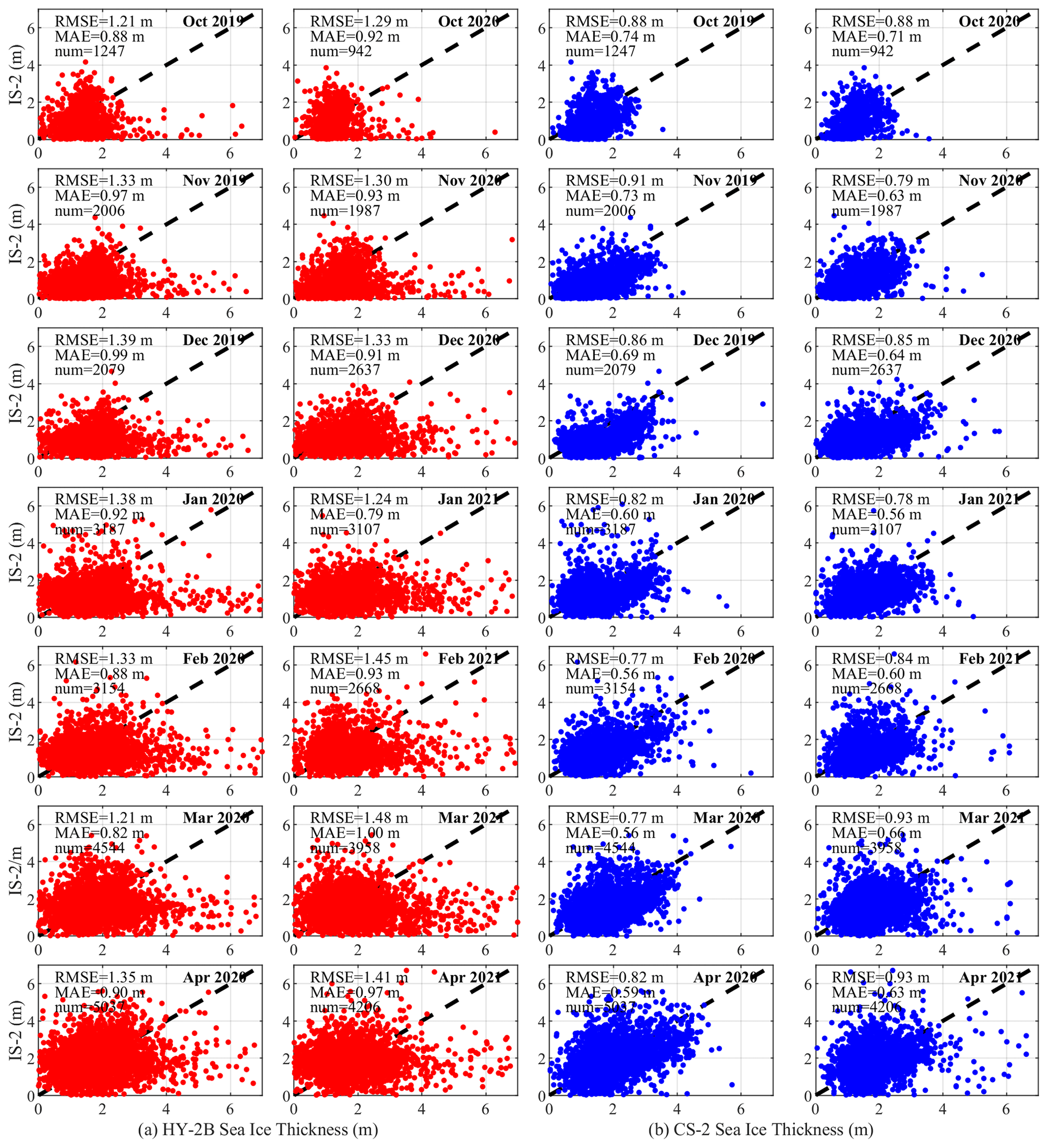
Figure 10Monthly comparisons between HY-2B sea ice thickness and ICESat-2 sea ice thickness and between CryoSat-2 sea ice thickness and ICESat-2 sea ice thickness: panel (a) shows comparisons between HY-2B and ICESat-2 in red points, and panel (b) shows comparisons between CS-2 and ICESat-2 in blue points.
Figure 11 shows the comparison of HY-2B sea ice freeboard uncertainty and AWI CS-2 sea ice freeboard uncertainty from October 2019 to April 2020 and October 2020 to April 2021. The spatial distributions of HY-2B sea ice freeboard uncertainty are similar to those of CS-2. The sea ice freeboard uncertainties over MYI are greater than those over FYI for HY-2B and CS-2, as the FYI snow depth and uncertainty values have been halved. In Table 9, we summarize the averages of sea ice freeboard uncertainty derived from HY-2B and CS-2 over the common area. The HY-2B sea ice freeboard uncertainty values range from 0.021 to 0.027 m, while the CS-2 sea ice freeboard uncertainty values range from 0.022 to 0.028 m.
Table 8Table of differences between CryoSat-2 radar freeboard and HY-2B radar freeboard retrieved by different SSHA determination schemes.
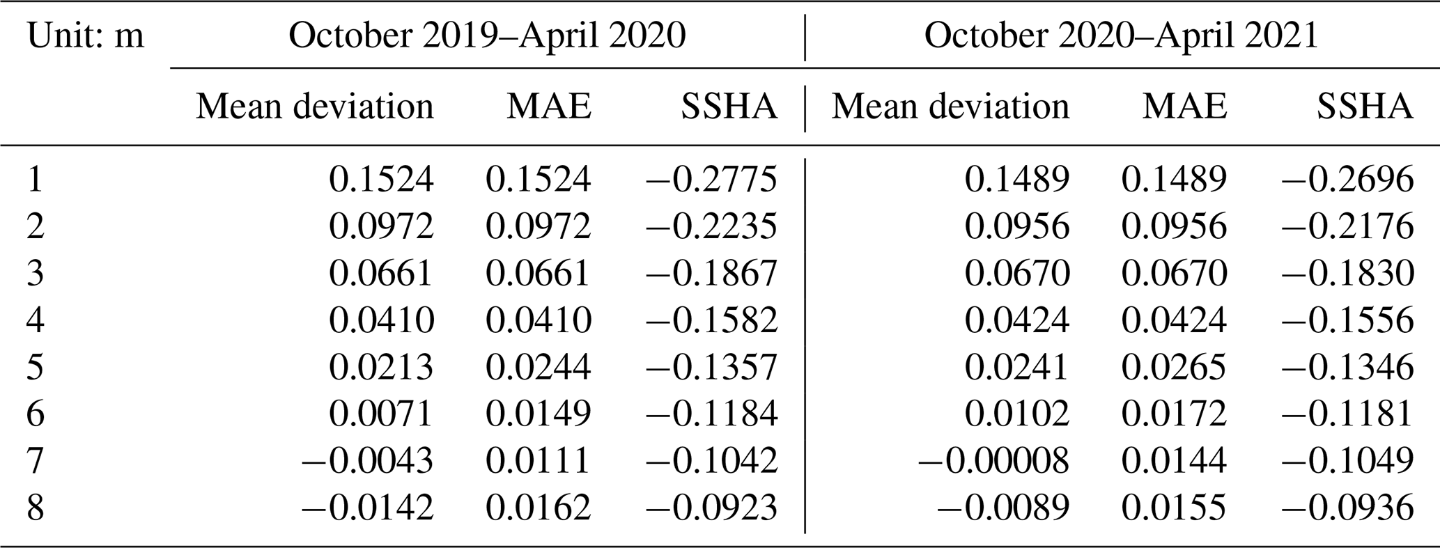
Table 9Mean sea ice freeboard uncertainties of HY-2B and CryoSat-2 on FYI, MYI and total sea ice.
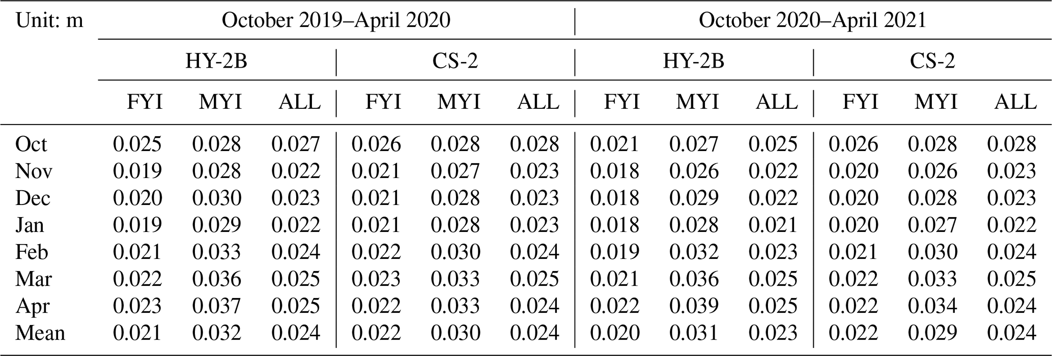
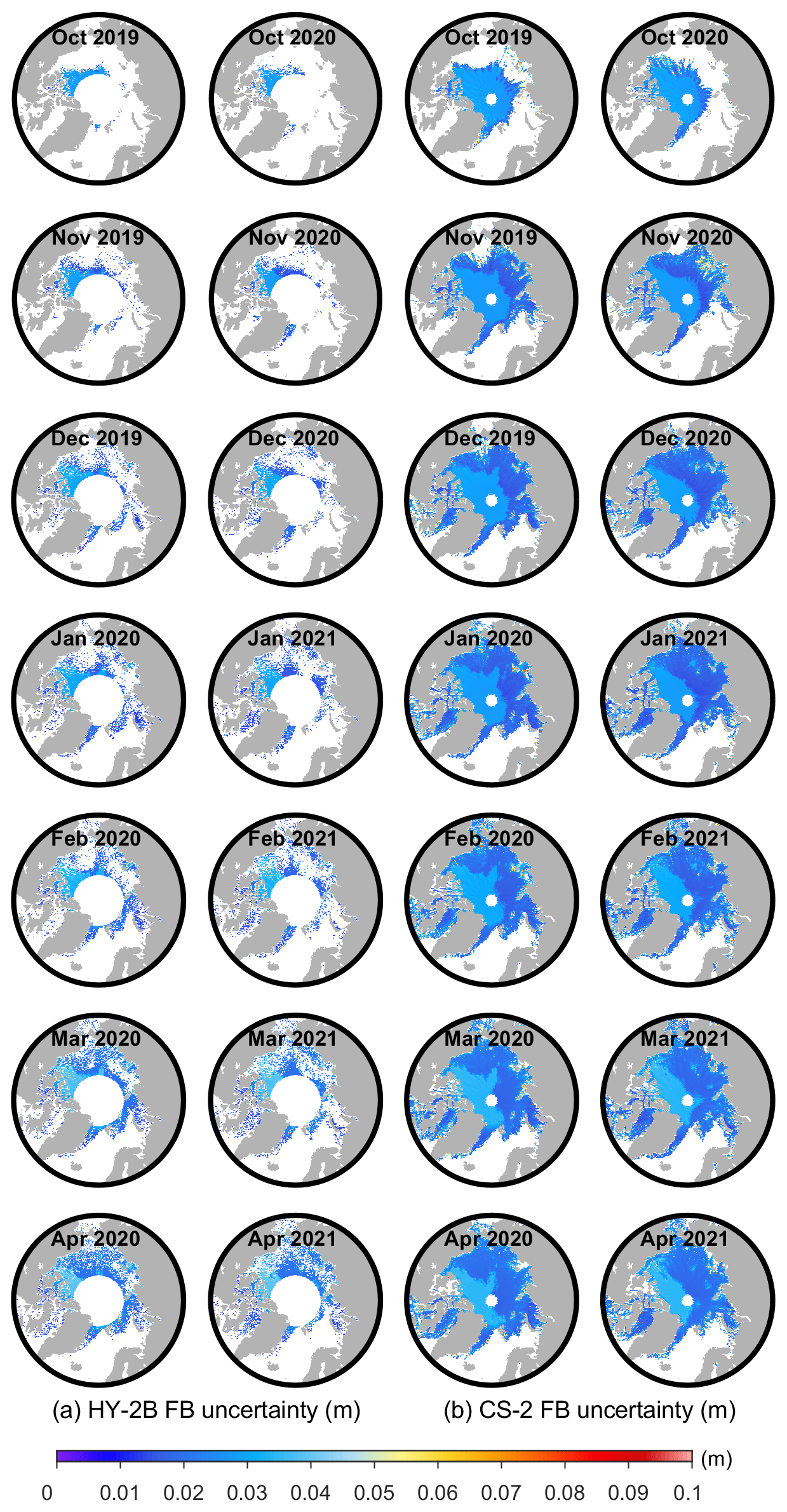
Figure 11Monthly comparisons between HY-2B sea ice freeboard uncertainties and CS-2 sea ice freeboard uncertainties from October 2019 to April 2020 and from October 2020 to April 2021: panel (a) shows the HY-2B sea ice freeboard uncertainties, and panel (b) shows the CS-2 sea ice freeboard uncertainties.
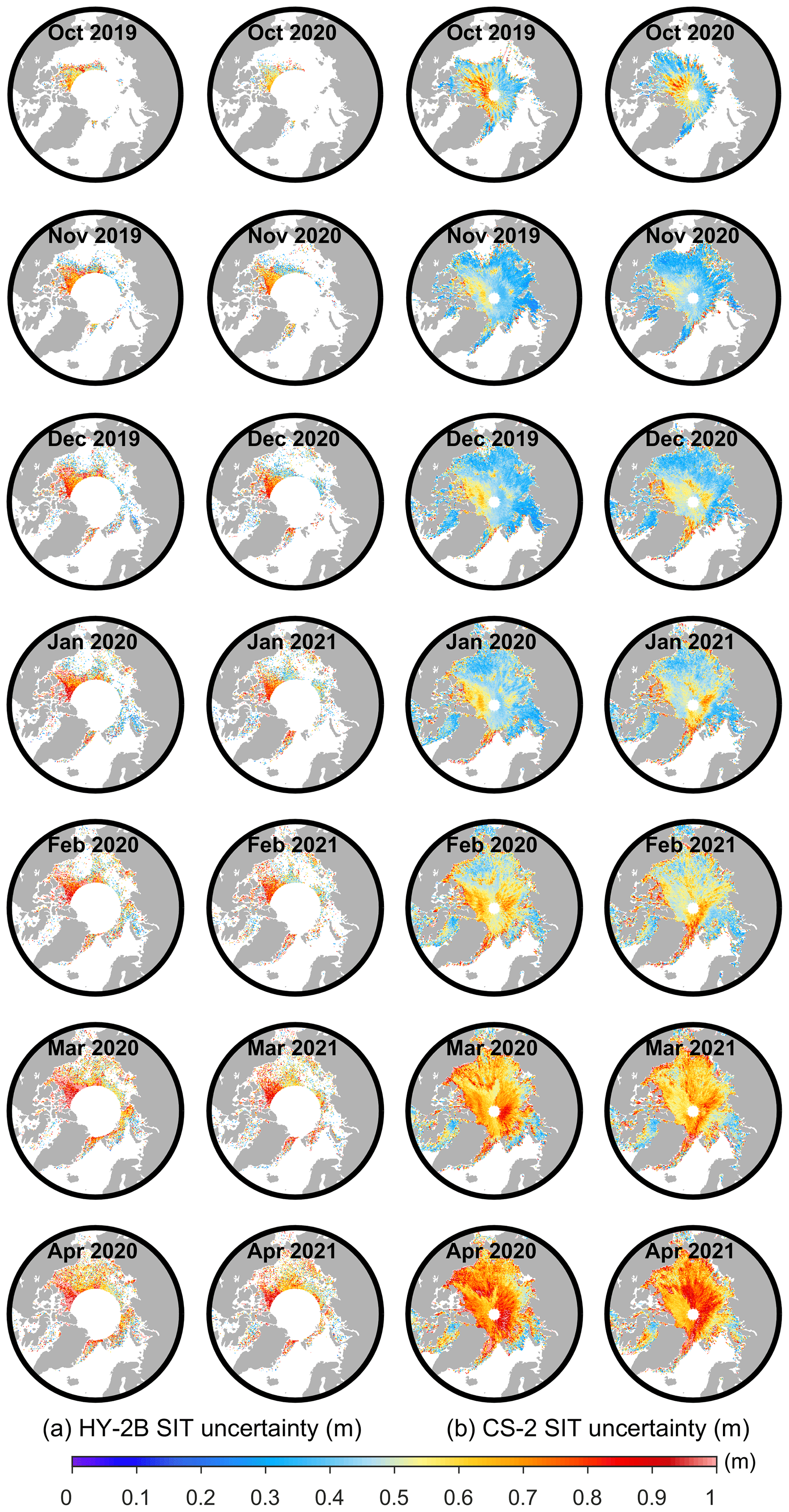
Figure 12Monthly comparisons between HY-2B sea ice thickness uncertainties and CS-2 sea ice thickness uncertainties from October 2019 to April 2020 and from October 2020 to April 2021: panel (a) shows the HY-2B sea ice thickness uncertainties, and panel (b) shows the CS-2 sea ice thickness uncertainties.
Figure 12 shows the comparison of the HY-2B sea ice thickness uncertainty and AWI CS-2 sea ice thickness uncertainty from October 2019 to April 2020 and from October 2020 to April 2021. The spatial distributions of the HY-2B sea ice thickness uncertainty are also similar to those of CS-2. The sea ice thickness uncertainties over MYI are greater than those over FYI for HY-2B and CS-2. In addition, the total error in the HY-2B and CS-2 sea ice thickness estimates increases as ice thickness increases over the growth season. Snow depth is a major contributor to this growth in sea ice thickness error, as snow accumulates and the associated standard deviation of depth anomalies increases (Tilling et al., 2019). Over FYI in October, the sea ice thickness uncertainty generated by SSHA is a dominant contributor to the error budget for HY-2B and CS-2. As the growth season progresses, its influence decreases as more measurements become available, and snow depth uncertainties become more significant. Over MYI, snow depth is the dominant contributing factor to the ice thickness error throughout the growth season for both HY-2B and CS-2 (Tilling et al., 2019). Table 10 summarizes the HY-2B sea ice freeboard uncertainty and CS-2 sea ice freeboard uncertainty over the common area. The HY-2B sea ice thickness uncertainties range from 0.61 to 0.74 m, while the CS-2 sea ice thickness uncertainties range from 0.42 to 0.69 m.
Table 10Mean sea ice thickness uncertainties of HY-2B and CryoSat-2 on FYI, MYI and total sea ice.
However, the uncertainties estimated in this study for both CS-2 and HY-2B are in the lower range when compared with other studies (Ricker et al., 2014; Landy et al., 2020). This is because we only calculate the statistics of uncertainty over the common area for CS-2 and HY-2B. Other studies do the statistics of CS-2 uncertainty with the upper limitation range of 88∘ N. In addition, Landy et al. (2020) also considered the following principal sources of systematic uncertainty: (i) partial wave penetration into the snowpack on MYI, for instance, due to metamorphic snow features; (ii) partial penetration into the snowpack on FYI, for instance, due to brine-wicking-induced snow basal salinity; and, finally, (iii) sea ice surface roughness. They revealed sea ice surface roughness as a key overlooked feature of the conventional retrieval process (Landy et al., 2020). It is important to note that these key uncertainties limit the accuracy of the radar-based freeboard retrieval, which then propagates into the freeboard-to-thickness conversion.
In this study, we first used the Chinese HY-2B radar altimeter to estimate Arctic sea ice freeboard and sea ice thickness with a new retrieval method and then compared the results to the AWI CS-2 products recorded during the same period. The accuracy of the findings was verified with independent data sources, including NASA OIB airborne data and IS-2 laser altimeter data. Finally, the uncertainties in the HY-2B sea ice freeboard and sea ice thickness were estimated. The main conclusions are as follows.
-
The spatial distributions of the HY-2B radar freeboard and AWI CS-2 radar freeboard have good consistency, but there are still some differences in the numerical values and temporal evolution. The HY-2B radar freeboards are generally thicker than those of AWI CS-2, except in spring (March and April). A spring segment likely has more floe points than an early winter segment. Therefore, the radar freeboards in spring are lower than those of CS-2. The mean deviations of the radar freeboard between HY-2B and AWI CS-2 range from −0.035 to 0.016 m from October 2019 to April 2020. The HY-2B radar freeboards are generally higher than AWI CS-2 in the FYI region and lower than AWI CS-2 in the MYI region. More of the lowest 15 points within the 25 km segment are likely to originate from floes in the MYI region, and more points may originate from leads in the FYI region. Therefore, the radar freeboard in the MYI region is lower than that of CS-2. Overall, the HY-2B radar freeboard is highly dependent on season and ice type. The radar freeboard deviation between HY-2B and AWI CS-2 over MYI is larger than that over FYI, with deviations of approximately 3 cm on FYI (positive) and 5 cm on MYI (negative). In addition, the growth trend of the HY-2B radar freeboard is slower than that of AWI CS-2.
Similarly, the spatial distributions of the HY-2B sea ice thickness and AWI CS-2 data exhibited good consistency, but we still identified some differences in their numerical and temporal evolution patterns. The mean deviations in sea ice thickness between HY-2B and AWI CS-2 range from −0.259 to 0.230 m from October 2019 to April 2020. Due to the lower radar freeboards in spring than those of CS-2, the sea ice thicknesses are also lower in spring than those of CS-2. In the FYI region, the HY-2B sea ice thicknesses are generally higher than those of AWI CS-2 and lower than those of AWI CS-2 in the MYI region. The sea ice thickness deviation between HY-2B and AWI CS-2 over MYI is larger than that over FYI, with deviations of approximately 0.3 m on FYI (positive) and 0.4 m on MYI (negative). The HY-2B sea ice thickness also has a smaller linear growth rate than CS-2.
-
Comparisons with the OIB obtained in April 2019 showed that the correlation between HY-2B sea ice freeboard retrievals and OIB values is 0.77, with an RMSE of 0.13 m and an MAE of 0.12 m. The correlation between HY-2B sea ice thickness retrievals and OIB values is 0.65, with an RMSE of 1.86 m and an MAE of 1.72 m. The majority of the spread in our HY-2B evaluation is caused by HY-2B underestimating sea ice thickness compared with OIB over thick ice. Moreover, the RMSEs between our HY-2B radar freeboard estimates and IS-2 range from 0.13 to 0.16 m, and the MAEs range from 0.09 to 0.12 m. The RMSEs between our HY-2B sea ice thickness estimates and IS-2 range from 1.21 to 1.48 m, and the MAEs range from 0.79 to 1.00 m. The abnormal values from HY-2B may be caused by the error of orbit determination, the Brown tracking algorithm and the determination algorithm of SSHA.
-
Based on Gaussian error propagation theory, we estimate the uncertainties in the HY-2B sea ice freeboard and sea ice thickness. The HY-2B sea ice freeboard uncertainty values range from 0.021 to 0.027 m, while the uncertainties in the HY-2B sea ice thickness range from 0.61 to 0.74 m. The HY-2B sea ice freeboard uncertainties over MYI are greater than those over FYI, as the FYI snow depth and uncertainty values have been halved. The total error in the HY-2B sea ice thickness estimates increases as the ice thickness increases over the growth season. Snow depth is a major contributor to this growth in sea ice thickness error, as snow accumulates and the associated standard deviation of depth anomaly increases.
However, we are aiming to investigate whether HY-2B can be used for sea ice, but we are limited to the already provided higher-level (SGDR) product, and it is not within the scope of the study to derive the freeboard product using our own retracker from the HY-2B SGDR product. The deficiency of this work is that we did not accurately distinguish between floes and lead. Moreover, the discrepancies between this study and Jiang et al. (2023) are mainly due to retrieval methods and data sources. The discrepancies of the methods are reflected in the retracking method, the estimation method of SSHA and whether the subsequent results need to be calibrated with AWI CS-2. The discrepancies of the datasets are reflected in product levels of HY-2B and DTU MSS models. Jiang et al. (2023) used the lowest three points per 25 km to estimate SSHA with HY-2B L1 product, and the resulting retrieval of sea ice thickness is thicker than AWI CS-2. So the retrieval of sea ice thickness needs to be calibrated with AWI CS-2. It is worth noting that this study uses SGDR data, which only include the SMLE retracking data. We do not deny that the L1 data Jiang et al. (2023) used are much more extensive in the Arctic. In this study, we try to explore the application of SGDR data released to the public in polar sea ice, but it can be seen from our study that it seems difficult to obtain reasonable results by using conventional methods. So we use the 15 lowest points per 25 km to estimate SSHA to retrieve more reasonable Arctic radar freeboard and thickness. Through this study, we can see that the relative surface height after subtracting MSS is relatively low compared with CS-2, which may be caused by the retracking algorithm and precision orbit determination. This is what we need to avoid when reprocessing HY-2B L1 data, which also provides reference for reprocessing L1 data. We will develop a higher-accuracy classification algorithm to classify floes and lead and use this improved algorithm to retrieve sea ice freeboard and sea ice thickness. We will use an implementation of the threshold first maximum retracker algorithm (TFMRA) to estimate the range to the main scattering horizon for each waveform. In addition, the HY-2B SGDR data used in this work retained only the measurements of the suboptimal-maximum-likelihood-estimation (SMLE) retracking algorithm, which is applicable only to the ocean surface. Although the offset-centre-of-gravity (OCOG) retracking algorithm is applicable to non-ocean surfaces, including land and sea ice, it is not saved in SGDR data and thus needs to be obtained from HY-2B L1 data. It is necessary to recalculate the satellite altitude using fine-orbit determination data and recalculate various geophysical correction terms, including the wet and dry troposphere correction, ionospheric correction, ocean tidal correction, polar tide correction, and earth tide correction terms. We hope to release products that are more reasonable and suitable for polar sea ice thickness retrieval, so as to better evaluate the potential application of HY-2B in polar sea ice.
The HY-2B SGDR data are available at ftp://osdds-ftp.nsoas.org.cn/ provided by NSOAS (2022a). If you have not registered before, you will need to create an account to access the FTP server at this website (https://osdds.nsoas.org.cn/register, last access: 30 June 2022). Then, you can enter your account and password to log in to the official website to access the FTP folder with SGDR HY-2B data using FileZilla (ftp://osdds-ftp.nsoas.org.cn/, last access: 30 June 2022). The SGDR HY-2B data can also be accessed through https://osdds.nsoas.org.cn/MarineDynamic/ (NSOAS, 2022b). The radar freeboard and sea ice thickness data corresponding to CryoSat-2 level 2I are available at ftp://science-pds.cryosat.esa.int/, provided by the ESA (last access: 30 June 2022). CryoSat-2 radar freeboard, sea ice thickness and snow depth data are available at ftp://ftp.awi.de/sea_ice/ (last access: 30 June 2022), provided by the AWI (Ricker et al., 2014; Hendricks and Ricker, 2020). The ATL20 products (version 003) for the ICESat-2 laser altimeter are available at https://doi.org/10.5067/ATLAS/ATL20.003, provided by the NSIDC (Petty et al., 2021). The IceBridge level-4 data (IDCSI4) are available at https://nsidc.org/data/NSIDC-0708/versions/1/ (last access: 30 June 2022), provided by the NSIDC (Kurtz et al., 2013). The sea ice concentration and sea ice type data are available at https://osi-saf.eumetsat.int (last access: 30 June 2022), provided by the OSI-SAF (Tonboe et al., 2016; Aaboe et al., 2021). The DTU18 MSS data are available at ftp://ftp.space.dtu.dk/pub/ (last access: 30 June 2022), provided by the DTU (Andersen et al., 2018a, b).
Data curation: ZD, YJ and LS; writing: ZD and LS; methodology: ZD, LS, ML, YJ, TZ and SW; validation: ZD, TZ and SW; funding acquisition: LS and ML. All authors have read and agreed to the published version of the paper.
The contact author has declared that none of the authors has any competing interests.
Publisher's note: Copernicus Publications remains neutral with regard to jurisdictional claims in published maps and institutional affiliations.
The authors would like to thank the editors and reviewers for their invaluable efforts in improving the paper. The authors would also like to thank the NSOAS, ESA, NSIDC, AWI, OSI-SAF and DTU for providing all the data needed for this paper.
The research is funded by the National Key Research and Development Program of China (grant numbers 2021YFC2803300 and 2018YFC1407200) and the Impact and Response of Antarctic Seas to Climate Change programme (grant number IRASCC2020-2022-No. 01-01-03).
This paper was edited by Vishnu Nandan and reviewed by Rasmus Tage Tonboe and two anonymous referees.
Aaboe, S., Down, E., and Eastwood, S.: Global Sea Ice Edge (OSI-402-d) and Type (OSI-403-d) Validation Report, v3.1, in: SAF/OSI/CDOP3/MET-Norway/SCI/RP/224, EUMETSAT OSISAF–Ocean and Sea Ice Satellite Application Facility, 2021.
Alexandrov, V., Sandven, S., Wahlin, J., and Johannessen, O. M.: The relation between sea ice thickness and freeboard in the Arctic, The Cryosphere, 4, 373–380, https://doi.org/10.5194/tc-4-373-2010, 2010.
Andersen, O. B., Knudsen, P., and Stenseng, L.: A New DTU18 MSS Mean Sea Surface – Improvement from SAR Altimetry, 172, in: Proceedings of the 25 years of progress in radar altimetry symposium, Ponta Delgada, São Miguel Island, Portugal, 24–29 September 2018, edited by: Benveniste, J. and Bonnefond, F., Azores Archipelago, Portugal, 172, 24–26, https://orbit.dtu.dk/en/publications/a-new-dtu18-mss-mean-sea-surface-improvement-from-sar-altimetry (last access: 30 June 2022), 2018a.
Andersen, O. B., Rose, S. K., Knudsen, P., and Stenseng, L.: The DTU18 MSS Mean Sea Surface Improvement from SAR Altimetry, in: International Symposium of Gravity, Geoid and Height Systems (GGHS) 2, The second joint meeting of the International Gravity Field Service and Commission 2 of the International Association of Geodesy, Copenhagen, Denmark, 17–21, https://orbit.dtu.dk/en/publications/a-new-dtu18-mss-mean-sea-surface-improvement-from-sar-altimetry (last access: 30 June 2022, 2018b.
Beaven, S. G., Lockhart, G. L., Gogineni, S. P., Hossetnmostafa, A. R., Jezek, K., Gow, A. J., Perovich, D. K., Fung, A. K., and Tjuatja, S.: Laboratory measurements of radar backscatter from bare and snow covered saline ice sheets, Int. J. Remote Sens., 16, 851–876, https://doi.org/10.1080/01431169508954448, 1995.
Cao, Y., Liang, S., Sun, L., Liu, J., Cheng, X., Wang, D., Chen, Y., Yu, M., and Feng, K.: Trans-Arctic shipping routes expanding faster than the model projections, Global Environmental Change, 73, 102488, https://doi.org/10.1016/j.gloenvcha.2022.102488, 2022.
Cartwright, D. E. and Edden, A. C.: Corrected Tables of Tidal Harmonics, Geophys. J. Int., 33, 253–264, https://doi.org/10.1111/j.1365-246X.1973.tb03420.x, 1973.
Comiso, J. C., Parkinson, C. L., Gersten, R., and Stock, L.: Accelerated decline in the Arctic sea ice cover, Geophys. Res. Lett., 35, L01703, https://doi.org/10.1029/2007gl031972, 2008.
Degnan, J. J.: Photon-counting multikilohertz microlaser altimeters for airborne and spaceborne topographic measurements, J. Geodyn., 34, 503–549, https://doi.org/10.1016/s0264-3707(02)00045-5, 2002.
Drinkwater, M. R., Hosseinmostafa, R., and Gogineni, P.: C-band backscatter measurements of winter sea-ice in the Weddell Sea, Antarctica, Int. J. Remote Sens., 16, 3365–3389, https://doi.org/10.1080/01431169508954635, 1995.
ESA: CryoSat-2 Product, ftp://science-pds.cryosat.esa.int/, last access: 30 June 2022.
Fons, S. W., Kurtz, N. T., Bagnardi, M., Petty, A. A., and Tilling, R. L.: Assessing CryoSat-2 Antarctic snow freeboard retrievals using data from ICESat-2, Earth Space Sci., 8, e2021EA001728, https://doi.org/10.1029/2021EA001728, 2021.
Giles, K. A., Laxon, S. W., Wingham, D. J., Wallis, D. W., Krabill, W. B., Leuschen, C. J., McAdoo, D., Manizade, S. S., and Raney, R. K.: Combined airborne laser and radar altimeter measurements over the Fram Strait in May 2002, Remote Sens. Environ., 111, 182–194, https://doi.org/10.1016/j.rse.2007.02.037, 2007.
Giles, K. A., Laxon, S. W., and Ridout, A. L.: Circumpolar thinning of Arctic sea ice following the 2007 record ice extent minimum, Geophys. Res. Lett., 35, L22502, https://doi.org/10.1029/2008gl035710, 2008.
Glissenaar, I. A., Landy, J. C., Petty, A. A., Kurtz, N. T., and Stroeve, J. C.: Impacts of snow data and processing methods on the interpretation of long-term changes in Baffin Bay early spring sea ice thickness, The Cryosphere, 15, 4909–4927, https://doi.org/10.5194/tc-15-4909-2021, 2021.
Hendricks, S. and Ricker, R.: Product User Guide & Algorithm Specification – AWI CryoSat-2 Sea Ice Thickness (version 2.3), https://www.researchgate.net/publication/346677382 (last access: 30 June 2022), 2020.
IPCC: Climate Change 2022: Impacts, Adaptation and Vulnerability. Contribution of Working Group II to the Sixth Assessment Report of the Intergovernmental Panel on Climate Change, edited by: Pörtner, H.-O., Roberts, D. C., Tignor, M., Poloczanska, E. S., Mintenbeck, K., Alegría, A., Craig, M., Langsdorf, S., Löschke, S., Möller, V., Okem, A., and Rama, B., Cambridge University Press. Cambridge University Press, Cambridge, UK and New York, NY, USA, 3056 pp., https://report.ipcc.ch/ar6/wg2/IPCC_AR6_WGII_FullReport.pdf (last access: 27 March 2023), 2022.
Jiang, C., Lin, M., and Wei, H.: A Study of the Technology Used to Distinguish Sea Ice and Seawater on the Haiyang-2A/B (HY-2A/B) Altimeter Data, Remote Sens., 11, 1490, https://doi.org/10.3390/rs11121490, 2019.
Jiang, M., Xu, K., Zhong, W., and Jia, Y.: Preliminary HY-2B Radar Freeboard Retrieval Over Arctic Sea Ice, IGARSS 2022 – 2022 IEEE International Geoscience and Remote Sensing Symposium, Kuala Lumpur, Malaysia, 2022, 3904–3907, https://doi.org/10.1109/IGARSS46834.2022.9883529, 2022.
Jiang, M., Zhong, W., Xu, K., and Jia, Y. :Estimation of Arctic Sea Ice Thickness from Chinese HY-2B Radar Altimetry Data, Remote Sens., 15, 1180, https://doi.org/10.3390/rs15051180, 2023.
Kurtz, N. and Harbeck, J.: CryoSat-2 Level-4 Sea Ice Elevation, Freeboard, and Thickness, Version 1 [October–April, 2010–2018], NASA National Snow and Ice Data Center Distributed Active Archive Center [data set], Boulder, Colorado USA, https://doi.org/10.5067/96JO0KIFDAS8, 2017.
Kurtz, N., Studinger, M. S., Harbeck, J., Onana, V., and Farrell, S.: IceBridge Sea Ice Freeboard, Snow Depth, and Thickness in the Lincoln Sea, Northern Hemisphere, Tech. rep., Boulder, Colorado USA, NASA DAAC at the National Snow and Ice Data Center, 2012.
Kurtz, N. T., Farrell, S. L., Studinger, M., Galin, N., Harbeck, J. P., Lindsay, R., Onana, V. D., Panzer, B., and Sonntag, J. G.: Sea ice thickness, freeboard, and snow depth products from Operation IceBridge airborne data, The Cryosphere, 7, 1035–1056, https://doi.org/10.5194/tc-7-1035-2013, 2013.
Kurtz, N. T., Galin, N., and Studinger, M.: An improved CryoSat-2 sea ice freeboard retrieval algorithm through the use of waveform fitting, The Cryosphere, 8, 1217–1237, https://doi.org/10.5194/tc-8-1217-2014, 2014.
Kwok, R.: ICESat observations of Arctic sea ice: A first look, Geophys. Res. Lett., 31, L16401, https://doi.org/10.1029/2004gl020309, 2004.
Kwok, R.: Arctic sea ice thickness, volume, and multiyear ice coverage: Losses and coupled vari-ability (1958–2018), Environ. Res. Lett., 13, 105005, https://doi.org/10.1088/1748-9326/aae3ec, 2018.
Kwok, R. and Cunningham, G. F.: Variability of Arctic sea ice thickness and volume from CryoSat-2, Philos. T. Roy. Soc. A, 373, 20140157, https://doi.org/10.1098/rsta.2014.0157, 2015.
Kwok, R., Cunningham, G. F., Zwally, H. J., and Yi, D.: Ice, Cloud, and land Elevation Satellite (ICESat) over Arctic sea ice: Retrieval of freeboard, J. Geophys. Res., 112, C12013, https://doi.org/10.1029/2006jc003978, 2007.
Kwok, R., Petty, A. A., Bagnardi, M., Kurtz, N. T., Cunningham, G. F., Ivanoff, A., and Kacimi, S.: Refining the sea surface identification approach for determining freeboards in the ICESat-2 sea ice products, The Cryosphere, 15, 821–833, https://doi.org/10.5194/tc-15-821-2021, 2021.
Lawrence, I. R., Armitage, T. W. K., Tsamados, M. C., Stroeve, J. C., Dinardo, S., Ridout, A. L., Muir, A., Tilling, R. L., and Shepherd, A.: Extending the Arctic Sea Ice Freeboard and Sea Level Record with the Sentinel-3 Radar Altimeters, Adv. Space Res., https://doi.org/10.1016/j.asr.2019.10.011, 2019.
Landy, J. C., Petty, A. A., Tsamados, M., and Stroeve, J. C.: Sea ice roughness overlooked as a key source of uncertainty in CryoSat-2 ice freeboard retrievals, J. Geophys. Res.-Oceans, 125, e2019JC015820, https://doi.org/10.1029/2019JC015820, 2020.
Laxon, S., Peacock, N., and Smith, D.: High interannual variability of sea ice thickness in the Arctic region, Nature, 425, 947–950, https://doi.org/10.1038/nature02050, 2003.
Lindell, D. B. and Long, D. G.: Multiyear Arctic Sea Ice Classification Using OSCAT and QuikSCAT, IEEE T. Geosci. Remote, 54, 167–175, https://doi.org/10.1109/TGRS.2015.2452215, 2016.
Magruder, L. A., Brunt, K. M., and Alonzo, M.: Early ICESat-2 on-orbit geolocation validation using ground-based corner cube retro-reflectors, Remote Sens., 12, 3653, https://doi.org/10.3390/rs12213653, 2020.
Mallett, R. D. C., Lawrence, I. R., Stroeve, J. C., Landy, J. C., and Tsamados, M.: Brief communication: Conventional assumptions involving the speed of radar waves in snow introduce systematic underestimates to sea ice thickness and seasonal growth rate estimates, The Cryosphere, 14, 251–260, https://doi.org/10.5194/tc-14-251-2020, 2020.
Meier, W. N. and Stroeve, J.: An updated assessment of the changing Arctic sea ice cover, Oceanography, 35, 10–19, https://doi.org/10.5670/oceanog.2022.114, 2022.
Nab, C., Mallett, R., Gregory, W., Landy, J., Lawrence, I., Willatt, R., Stroeve, J., and Tsamados, T.: Synoptic variability in satellite altimeter-derived radar freeboard of Arctic sea ice, Geophys. Res. Lett., 50, e2022GL100696, https://doi.org/10.1029/2022GL100696, 2023.
Nandan, V ., Scharien, R. K., Geldsetzer, T., Kwok, R., Yackel, J. J., Mahmud, M. S., and Stroeve, J.: Snow Property Controls on Modeled Ku-Band Altimeter Estimates of First Year Sea Ice Thickness: Case studies from the Canadian and Norwegian Arctic, IEEE J. Sel. Top. Appl., 13, 1082–1096, https://doi.org/10.1109/JSTARS.2020.2966432, 2020.
National Satellite Ocean Application Service (NSOAS): Instructions for HY-2B Satellite Data, https://osdds.nsoas.org.cn/HY2B_introduce (last access: 30 June 2022), 2019.
Notz, D. and SIMIP Community: Arctic sea ice in CMIP6, Geophys. Res. Lett., 47, e2019GL086749, https://doi.org/10.1029/2019GL086749, 2020.
NSOAS: HY-2B Product, ftp://osdds-ftp.nsoas.org.cn/, last access: 30 June 2022a.
NSOAS: HY-2B Product, https://osdds.nsoas.org.cn/MarineDynamic/, last access: 30 June 2022b.
Ollivier, A., Faugere, Y., Picot, N., Ablain, M., Femenias, P., and Benveniste, J.: Envisat Ocean Altimeter Becoming Relevant for Mean Sea Level Trend Studies, Mar. Geod., 35, 118–136, https://doi.org/10.1080/01490419.2012.721632, 2012.
Paul, S., Hendricks, S., and Rinne, E.: Sea Ice Climate Change Initiative Phase 2, D2.1 Sea Ice Thickness Algorithm Theoretical Basis Document (ATBD), SICCI-P2-ATBD (SIT), v.1.0, 50 pp., https://admin.climate.esa.int/media/documents/Sea_Ice_Thickness_Algorithm_Theoretical_Basis_Document_1.0.pdf (last access: September 2022), 2017.
Petty, A. A., Kurtz, N. T., Kwok, R., Markus, T., and Neumann, T. A.: Winter Arctic sea ice thickness from ICESat-2 freeboards, J. Geophys. Res.-Oceans, 125, e2019JC015764, https://doi.org/10.1029/2019JC015764, 2020.
Petty, A. A., Kwok, R., Bagnardi, M., Ivanoff, A., Kurtz, N., Lee, J., Wimert, J., and Hancock, D.: ATLAS/ICESat-2 L3B Daily and Monthly Gridded Sea Ice Freeboard, Version 3, Boulder, Colorado USA, NASA National Snow and Ice Data Center Distributed Active Archive Center [data set], https://doi.org/10.5067/ATLAS/ATL20.003, 2021.
Ricker, R., Hendricks, S., Helm, V., Skourup, H., and Davidson, M.: Sensitivity of CryoSat-2 Arctic sea-ice freeboard and thickness on radar-waveform interpretation, The Cryosphere, 8, 1607–1622, https://doi.org/10.5194/tc-8-1607-2014, 2014.
Sallila, H., Farrell, S. L., McCurry, J., and Rinne, E.: Assessment of contemporary satellite sea ice thickness products for Arctic sea ice, The Cryosphere, 13, 1187–1213, https://doi.org/10.5194/tc-13-1187-2019, 2019.
Schwegmann, S., Rinne, E., Ricker, R., Hendricks, S., and Helm, V.: About the consistency between Envisat and CryoSat-2 radar freeboard retrieval over Antarctic sea ice, The Cryosphere, 10, 1415–1425, https://doi.org/10.5194/tc-10-1415-2016, 2016.
Serreze, M. C., Barrett, A. P., Stroeve, J. C., Kindig, D. N., and Holland, M. M.: The emergence of surface-based Arctic amplification, The Cryosphere, 3, 11–19, https://doi.org/10.5194/tc-3-11-2009, 2009.
Shen, X., Ke, C., Xie, H., Li, M., and Xia, W.: A comparison of Arctic sea ice freeboard products from Sentinel-3A and CryoSat-2 data, Int. J.Remote Sens., 41, 2789–2806, https://doi.org/10.1080/01431161.2019.1698078, 2020.
Skourup, H., Farrell, S. L., Hendricks, S., Ricker, R., Armitage, T. W. K., Ridout, A., and Baker, S.: An assessment of state-of-the-art mean sea surface and geoid models of the Arctic Ocean: Implications for sea ice freeboard retrieval, J. Geophys. Res.-ceans, 122, 8593–8613, https://doi.org/10.1002/2017JC013176, 2017.
Stephenson, S. R. and Smith, L. C.: Influence of climate model variability on projected Arctic shipping futures, Earth's Future, 3, 331–343, https://doi.org/10.1002/2015EF000317, 2015.
Stroeve, J., Nandan, V., Willatt, R., Tonboe, R., Hendricks, S., Ricker, R., Mead, J., Mallett, R., Huntemann, M., Itkin, P., Schneebeli, M., Krampe, D., Spreen, G., Wilkinson, J., Matero, I., Hoppmann, M., and Tsamados, M.: Surface-based Ku- and Ka-band polarimetric radar for sea ice studies , The Cryosphere, 14, 4405–4426, https://doi.org/10.5194/tc-14-4405-2020, 2020.
Thomas, D. N. and Dieckmann, G. S.: Sea Ice, 2nd Edn., Wiley-Blackwell, Oxford, UK, https://doi.org/10.1002/9781444317145, 2010.
Tilling, R. L., Ridout, A., and Shepherd, A.: Near-real-time Arctic sea ice thickness and volume from CryoSat-2, The Cryosphere, 10, 2003–2012, https://doi.org/10.5194/tc-10-2003-2016, 2016.
Tilling, R. L., Ridout, A., and Shepherd, A.: Estimating Arctic sea ice thickness and volume using CryoSat-2 radar altimeter data, Adv. Space Res., 62, 1203–1225, https://doi.org/10.1016/j.asr.2017.10.051, 2017.
Tilling, R., Ridout, A., and Shepherd, A.: Assessing the impact of lead and floe sampling on Arctic sea ice thickness estimates from Envisat and CryoSat-2, J. Geophys. Res.-Oceans, 124, 7473–7485, https://doi.org/10.1029/2019JC015232, 2019.
Tonboe, R. and Lavelle, J.: The EUMETSAT OSI SAF Sea Ice Concentration Algorithm Theoretical Basis Document Product, OSI-401-b, Version 1.5, The Ocean and Sea Ice Satellite Application Facility, https://osisaf-hl.met.no/sites/osisaf-hl.met.no/files/baseline_document/osisaf_cdop2_ss2_atbd_amsr2-sea-ice-conc_v1p1.pdf (last access: 30 June 2022), 2016.
Tonboe, R. T., Toudal Pedersen, L., and Haas, C.: Simulation of the CryoSat-2 satellite radar altimeter sea ice thickness retrieval uncertainty, Can. J. Remote Sens., 36, 55–67, https://doi.org/10.5589/m10-027, 2010.
Ulaby, F., Moore, R., and Fung, A.: Microwave remote sensing: active and passive, Volume 3 – From Theory to Applications, Artech House, Norwood, Massachusetts, USA, equation number: E.80, ISBN-13 978-0890061916, 1986.
Wahr, L. W.: Deformation of the earth induced by polar motion, J. Geophys. Res., 90, 9363–9368, https://doi.org/10.1029/JB090iB11p09363, 1985.
Warren, S. G., Rigor, I. G., Untersteiner, N., Radionov, V. F., Bryazgin, N. N., Aleksandrov, Y. I., and Colony, R.: Snow Depth on Arctic Sea Ice, J. Climate, 12, 1814–1829, https://doi.org/10.1175/1520-0442(1999)012<1814:SDOASI>2.0.CO;2, 1999.
Willatt, R., Laxon, S., Giles, K., Cullen, R., Haas, C., and Helm, V.: Ku-band radar penetration into snow cover on Arctic sea ice using airborne data, Ann. Glaciol., 52, 197–205, https://doi.org/10.3189/172756411795931589, 2011.
Willatt, R. C., Giles, K. A., Laxon, S. W., Stone-Drake, L., and Worby, A. P.: Field investigations of Ku-band radar penetration into snow cover on Antarctic sea ice, IEEE T. Geosci. Remote, 48, 365–372, https://doi.org/10.1109/TGRS.2009.2028237, 2010.
Xu, S., Zhou, L., Liu, J., Lu, H., and Wang, B.: Data Synergy between Altimetry and L-Band Passive Microwave Remote Sensing for the Retrieval of Sea Ice Parameters – A Theoretical Study of Methodology, Remote Sensing, 9, 1079. https://doi.org/10.3390/rs9101079, 2017.
Zhang, S., Xuan, Y., Li, J., Geng, T., Li, X., and Xiao, F.: Arctic Sea Ice Freeboard Retrieval from Envisat Altimetry Data, Remote Sens., 13 1414, https://doi.org/10.3390/rs13081414, 2021.
Zhang, S., Zhou, R., Jia, Y., Jin, T., and Kong, X.: Performance of HaiYang-2 Altimetric Data in Marine Gravity Research and a New Global Marine Gravity Model NSOAS22, Remote Sens., 14, 4322, https://doi.org/10.3390/rs14174322, 2022.