the Creative Commons Attribution 4.0 License.
the Creative Commons Attribution 4.0 License.
 | 22 Mar 2023
Analysis of microseismicity in sea ice with deep learning and Bayesian inference: application to high-resolution thickness monitoring
Ludovic Moreau
Léonard Seydoux
Jérôme Weiss
Michel Campillo
In the perspective of an upcoming seasonally ice-free Arctic, understanding the dynamics of sea ice in the changing climate is a major challenge in oceanography and climatology. In particular, the new generation of sea ice models will require fine parameterization of sea ice thickness and rheology. With the rapidly evolving state of sea ice, achieving better accuracy, as well as finer temporal and spatial resolutions of its thickness, will set new monitoring standards, with major scientific and geopolitical implications. Recent studies have shown the potential of passive seismology to monitor the thickness, density and elastic properties of sea ice with significantly reduced logistical constraints. For example, human intervention is no longer required, except to install and uninstall the geophones. Building on this approach, we introduce a methodology for estimating sea ice thickness with high spatial and temporal resolutions from the analysis of icequake waveforms. This methodology is based on a deep convolutional neural network for automatic clustering of the ambient seismicity recorded on sea ice, combined with a Bayesian inversion of the clustered waveforms. By applying this approach to seismic data recorded in March 2019 on fast ice in the Van Mijen Fjord (Svalbard), we observe the spatial clustering of icequake sources along the shoreline of the fjord. The ice thickness is shown to follow an increasing trend that is consistent with the evolution of temperatures during the 4 weeks of data recording. Comparing the energy of the icequakes with that of artificial seismic sources, we were able to derive a power law of icequake energy and to relate this energy to the size of the cracks that generate the icequakes.
- Article
(5797 KB) - Full-text XML
- BibTeX
- EndNote


With the rapidly evolving climate in polar regions, collecting field data is key for anticipating the major upcoming changes related to global warming. In particular, sea ice is an essential element of polar regions because of the role it plays in phytoplankton production (Mayot et al., 2020) and in several atmosphere–ice–ocean interactions. In the Arctic, the extent of sea ice in summer undergoes an important negative trend of about 12.6 % per decade, according to the National Snow and Ice Data Center (https://nsidc.org/arcticseaicenews/charctic-interactive-sea-ice-graph/, last access: 21 March 2023). In the Antarctic, Parkinson (2019) observed a weak positive trend of 1.5 % per decade. However, this positive trend should be mitigated by the outstanding and unprecedented decline in 2015–2017, which shows how vulnerable Antarctic sea ice is to both ocean warming and changes in large-scale atmospheric winds (Eayrs et al., 2019). This emphasizes the need for progress in research addressing the nature of these changes, their pace and their impact at the global scale. In this matter, a finer and more accurate description of the dynamics and thermodynamic processes of sea ice is needed.
Given the challenging logistics for accessing polar regions, most of the knowledge about sea ice extent and concentration comes from remote sensing and in particular microwave-radar imagery, which provides altimetric information, which can be converted to ice thickness. Sea ice thickness is an important parameter, for many reasons. For example, thick ice filters light more than thin ice; hence thickness influences phytoplankton production (Ardyna et al., 2014). Thicker ice is also more resilient to external forcing such as swell or wind forcing (Dumont, 2022). Hence in the research effort for monitoring the state of sea ice, much focus is given to improving the spatial resolution and accuracy of thickness estimations. Remote sensing methods rely on a conversion between the freeboard measurement into an ice thickness estimation. These methods suffer from a lack of in situ measurements to calibrate the estimations, which can have several sources of errors, such as the presence of the snow cover, as well as uncertainties in the freeboard, in the densities of ice and snow, etc. (Garnier et al., 2021).
Seismic methods have been shown to be good candidates for evaluating sea ice properties at the local scale, with very good accuracy and spatial resolution. The first seismic experiments on sea ice date back to the late 1950s, where the elastic constants and the thickness of sea ice were estimated from the velocity of the seismic waves traveling in the ice cover (Crary, 1954; Anderson, 1958; Hunkins, 1960). With the emergence of digital signal processing, methods based on Fourier analysis were made possible, allowing for more accurate inversions of the signals to recover both the ice thickness and its elastic properties (Yang and Giellis, 1994; Stein et al., 1998). However, collecting seismic data on sea ice has long remained too challenging for applications to sea ice monitoring. With the miniaturization of electronic components, the rapid progress in terms of battery life and the era of seismic-noise interferometry (Shapiro and Campillo, 2004; Sabra et al., 2005), it has become possible to collect data without the need of active, human-controlled sources and then to process them remotely (Marsan et al., 2019). Therefore, over the past decade, there has been a renewed interest in seismic methods as a complementary means of monitoring the thickness, density and elastic properties of sea ice (Marsan et al., 2012; Moreau et al., 2020a, b; Romeyn et al., 2021; Serripierri et al., 2022).
The missing link between data acquisition and long-term sea ice monitoring is the ability to extract, in the continuous recordings, the useful parts of the seismic waveforms from the background noise, for automatic estimations of the sea ice properties. In this paper we combine a deep learning method for automatic clustering of the waveforms (Seydoux et al., 2020) recorded on sea ice with Bayesian inference to locate the position of thousands of icequakes while simultaneously evaluating the ice thickness. We demonstrate the possibility of generating maps of sea ice thickness and microseismic activity, with a temporal resolution that is directly linked to the number of icequakes recorded. In the specific configuration at the fjord, icequake occurrences are driven essentially by tide. On drifting ice, icequakes are generated by other mechanisms such as swell or ice motion, and many icequakes are also present in the ambient seismic field (Moreau et al., 2020b). With hundreds of icequakes recorded every day, a daily temporal resolution can be achieved. We also use the energy information to calculate the scaling law of icequakes in terms of their released energy.
2.1 Seismic array
In a thin structure such as sea ice, the seismic wavefield is multiply reflected at the upper and lower interfaces of the ice. These reflections interfere constructively to produce guided modes that propagate in the elongated direction of sea ice. When the product of the ice thickness by the frequency is larger than 1000 Hz m, the fundamental modes co-exist with higher-order modes in the wavefield (Moreau et al., 2017). Here, we restrict our analyses to frequency × thickness values, where only the fundamental modes are propagating. We use the terminology introduced in Moreau et al. (2020a) for referring to the following three modes:
-
the quasi-Scholte mode (QS), also known in the low-frequency regime as the flexural gravity wave;
-
the fundamental quasi-symmetric mode (QS0), also known in the low-frequency regime as the longitudinal wave;
-
the fundamental shear-horizontal mode (SH0), which produces shear-horizontal motion.
The QS mode is highly dispersive at low frequencies; hence seismic signals recorded in sea ice away from the source are distorted. It is noteworthy that the SH0 mode is not dispersive and that the QS0 becomes dispersive only at higher frequencies. An important property of guided-wave propagation is that given a set of ice mechanical properties, there is a direct relationship between the dispersion of the waveforms, the waveguide thickness and the source–receiver distance. By recording the seismic wavefield in sea ice, it is therefore possible to recover the structural information of the ice. In the frequency regime of interest here, only the QS mode is dispersive, and it has most of its energy on the vertical component of the displacement, while the QS0 and SH0 modes are not dispersive and have energy mainly on the horizontal components of the displacement.
To record the seismic wavefield in sea ice, an experiment was conducted on fast ice in Svalbard (Norway), in a specific part of the Van Mijen Fjord called Lake Vallunden (Fig. 1a). This part of the fjord is surrounded by moraines and can therefore be regarded as a “lake connected to the fjord”, with a depth of about 10 m (Marchenko and Morozov, 2013). A dense array of 247 geophones was deployed and left to record seismic noise for 1 month. For a detailed description of the dense array, we refer the reader to Moreau et al. (2020a). In the present study, however, we use only five geophones of the dense array, as shown in Fig. 1b as stations Si (i=1, 2, …, 5). Fast ice in this part of the fjord was continuous, with cracks located for the most part along the shoreline, which indicates that they are likely tide cracks.

Figure 1(a) Map of the area where the seismic array was installed (black squares) on Lake Vallunden, Svalbard. It is naturally bounded by moraines and connected to the Van Mijen Fjord by a small channel. The facilities of Sveagruva are located about 1.5 km west of the deployment. (b) Zoom on the five seismic stations (Si, where i=1, 2, …, 5) used to record the ambient seismic field. Arrows indicate the positions of ice drillings (ID). ID1 was performed on 1 March, giving a thickness of 62 cm; ID2 and ID3 were performed on 26 March, giving thicknesses of 70 and 73 cm.
The data in this paper were recorded using FairFieldNodal Zland three-component geophones. These all-in-one sensors have an internal battery, a built-in GPS and flash memory to store the data, allowing for several weeks of autonomous and continuous recording, without the need of external cables. They have a cylindrical geometry of about 17 cm in height and 12 cm in diameter and are mounted on a detachable spike. They were installed directly in the ice without their spike. To maximize the coupling, a milling tool was specifically designed to drill the ice at the diameter of the nodes. The snow was removed prior to drilling holes, and geophones were installed in the holes at about half their height. We covered them back with snow to insulate them in view of preserving their battery life. At the time of the deployment, the internal temperature of several nodes was measured, before and after covering them with snow, showing an increase from −21 to −16 ∘C.
FairFieldNodal Zland three-component geophones have a flat frequency response down to their eigenfrequency of 5 Hz. We recorded the data with a sampling frequency of 1000 Hz (Moreau and RESIF, 2019), but in order to reduce the computational cost of the present study, data were downsampled at 250 Hz. Conversion of the raw data into a miniSEED (Standard for the Exchange of Earthquake Data) format was obtained using the Fairfield software. Instrument response deconvolution is not necessary for our methodology and was therefore not applied. Data are expressed in millivolts but could be converted to velocity by dividing by the proportionality factor of 89 V m−1 s−1 and further converted to displacement by integration with respect to time.
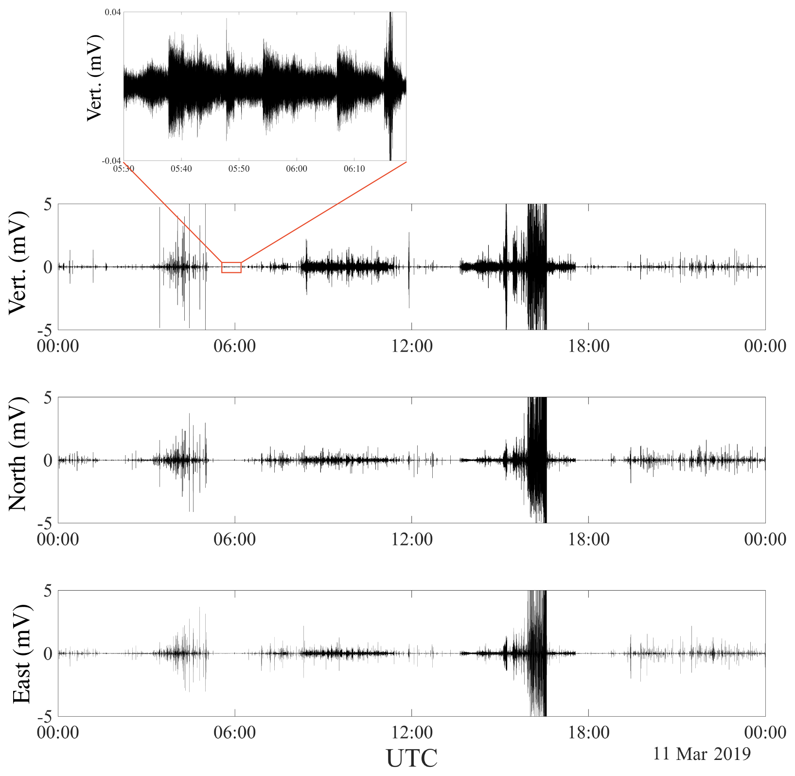
Figure 2The three 24 h waveform components of the ambient seismic field recorded on fast ice in Svalbard on 11 March 2019. The wavefield is very rich and composed of icequakes with different orders of energy magnitude, transients (see the zoomed area on the vertical channel) and anthropogenic activities (between 08:00 and 17:00).
2.2 Automatic clustering of the waveforms
In Moreau et al. (2020b), we introduced an approach based on a Bayesian inversion of the icequakes waveform to recover the ice thickness while simultaneously relocating the source position, after the Young's modulus and Poisson's ratio of the ice were estimated from noise interferometry. This method was validated on a few icequakes recorded in fast ice and in pack ice. In this paper we are using this approach to conduct a systematic analysis of the thousands of icequakes recorded at Lake Vallunden during the 1-month experiment.
Figure 2 shows 24 h of recording on 11 March 2019, at station S1 (see Fig. 1b). This typical recording exhibits various types of signals, including thousands of icequakes with several orders of magnitude of energy, long-lasting transients and background noise. Some waveforms are also related to anthropogenic activities. Therefore, the first processing step consists of extracting all icequakes from the recordings. Template matching is a common processing method for detecting similar waveforms in continuous recordings. However, although icequakes may look similar, their propagation in sea ice is accompanied by a strong dispersion of the quasi-Scholte mode. Hence, each combination of ice thickness and propagation distance results in a different waveform. For this reason, we use the scatseisnet algorithm, introduced by Seydoux et al. (2020), and we apply this clustering algorithm to the three components of the displacements recorded at S1.
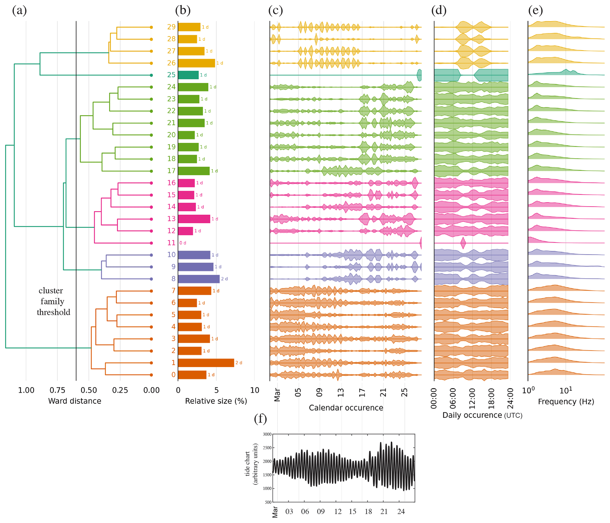
Figure 3(a) Hierarchical representation of the ambient seismic field after the scatseisnet algorithm was applied to the 27 d of continuous recording at station S1. A total of 6 families (shown as different colors) and 30 clusters are categorized. For each sub-family: (b) cumulated duration of the waveforms, (c) calendar occurrence, (d) time of day of occurrences and (e) spectrum of the waveforms. (f) Tide chart at the Ny-Ålesund station (∼160 km away from Lake Vallunden).
The scatseisnet algorithm is inspired by deep learning and automatically clusters segments of seismic data in continuous seismic records at a unique station.
It combines a deep scattering network (Andén and Mallat, 2014) to transform the seismic waveforms into a relevant data space to identify relevant features suitable for clustering.
The most relevant features are then extracted from the output of the deep scattering representation with an independent component analysis (Comon, 1992). A summary of these processing steps is given in Appendix B.
This strategy is applied on the segmented seismic time series, with a fixed window size of a few times the duration of the events of interest (see, e.g., Steinmann et al., 2022, for more information). For every signal segment, we obtain 20 real-valued features out of the independent component analysis. We finally use a hierarchical clustering approach to identify clusters of signal segments. By adjusting the distance threshold of the dendrogram (ward distance), we control the final number of clusters. A smaller distance implies a larger number of clusters. In the present case, apart from the transient waveforms lasting several minutes, the typical duration of the waveforms in our recording is of a few seconds. Since this study does not focus on the transient signals, we use a 40 s long sliding window with a 20 s overlap. We represent the hierarchical clustering output in the form of a dendrogram as in Fig. 3a, for data collected at station S1. This clustering would not change if applied to another stations, which is one of the advantages of using a deep scattering network. With the threshold distance indicated in the figure, we identify six families of signals, represented with different colors.
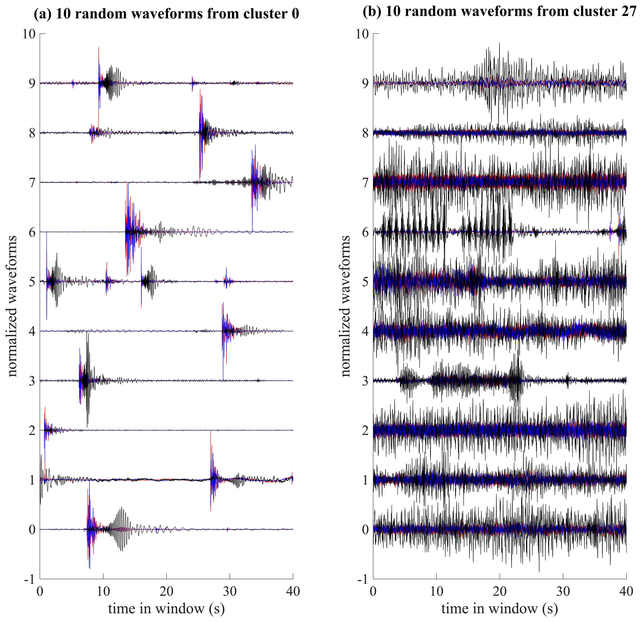
Figure 4(a) Random waveforms extracted from cluster 0, which contains mainly clean icequakes. (b) Random waveforms extracted from cluster 27, which contains mainly signals from anthropogenic activities. Black: vertical component, blue: axial component, red: transverse component of displacement.
The family with clusters referenced 0 to 7 (Fig. 3a) accounts for about 30 % of the dataset (Fig. 3b). Figure 4a shows 10 waveforms randomly sampled from cluster 0. We see that this cluster contains clean icequakes with a very good signal-to-noise ratio (SNR). So do the other six clusters of the first family. The icequakes have calendar occurrences every day of the deployment but are more frequent between 27 February and 13 March and then between 21 and 25 March (Fig. 3c). It is noteworthy that this is consistent with the tide chart shown in Fig. 3f and also with the fact that spring tides occurred on 6 and 21 March, while a neap tide occurred on 13 March. Icequakes occur at all times of the day with the same temporal distribution, except around 09:00, where occurrences slightly decreased (Fig. 3d). The decreased-occurrence rates in the latter half of March could be due to the thickening of the ice (∼25 % thickness increase).
Figure 3e indicates that the signals have a frequency content ranging between 1 and 50 Hz. To be more specific, on the vertical channel, dominated by the QS mode, the amplitude of the spectrum of icequake waveforms remains (on average) over −30 dB between 1 and 35 Hz, with a peak value around 8 Hz. On the horizontal channels, where the QS0 and SH0 modes are dominant, the spectrum remains over −30 dB up to 50 Hz.
Although some icequakes may be the consequence of thermomechanical forcing (Olinger et al., 2019), it is likely that the majority are tidal icequakes. The temperature log can be extracted from the Sveagruva weather station (SN99760), located 2 km west of the experiment location. Data for this station are available at https://seklima.met.no/hours/air_temperature/custom_period/SN99760/en/2019-02-27T00:00:00+01:00;2019-03-26T23:59:59+01:00 (last access: 21 March 2023). These temperatures are shown in Fig. 5. The absence of a periodic pattern in temperature variations suggests that tides have more effect on the generation of icequakes than changes in temperature. The majority of icequakes occur within a period of 24 h (Fig. 6). This periodicity can also be seen in Fig. 3c, especially between 1 and 15 March. One would expect the semidiurnal tide (10–20 cm) to reflect in the periodicity of the icequakes, but the specific geometry of the moraines around the experiment, together with the small channel that connects it to the fjord, generates some nonlinear effects that cause the tide in Lake Vallunden to be asymmetric (Marchenko and Morozov, 2013). This could explain why occurrences are dominated by a period of 24 h instead of 12 h.
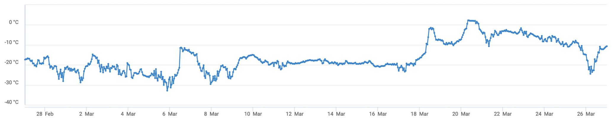
Figure 5Air temperature recorded during deployment at the Sveagruva weather station (SN99760, https://seklima.met.no/hours/air_temperature/custom_period/SN99760/en/2019-02-27T00:00:00+01:00;2019-03-26T23:59:59+01:00, last access: 21 March 2023), located about 2 km west of the experiment. Temperatures remained between −30 and −10 ∘C until 18 March and then remained essentially between −10 and 0 ∘C until the end of deployment, which is consistent with the dynamic of ice thickness shown in Fig. 7, which exhibits a sharp increase between 27 February and 16 March and then stabilizes.
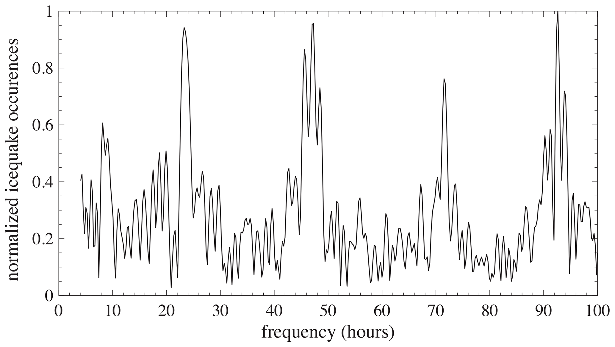
Figure 6Frequency of icequake occurrences, obtained by discrete Fourier transform of the dates of all icequakes in clusters 0–7 and normalized with the maximum amplitude in the resulting spectrum. The majority of icequakes occur within a period of 24 h and are therefore most likely linked to tidal forcing.
The family with clusters referenced 26 to 29 accounts for about 13 % of the dataset. Figure 4b shows 10 waveforms randomly sampled from cluster 27. The waveforms are more complex and include many impulsive events, some noise, repeating events and events that last up to 15–20 s. The waveforms in this family occur mostly during three sequences. The first sequence is between 27 February and 2 March, when we went into the field to deploy the geophones and performed field experiments, including impulsive sources, sweep sources and snowmobile driving. The second sequence is between 5 and 16 March, when a team of researchers and students were conducting field experiments about 150 m northeast of station S3 (Marchenko et al., 2021). The third sequence is between 25 and 27 March, when we went back for some more field experiments before removing the geophones. For a list of the exact times (coordinated universal time, UTC) of the impulsive and sweep sources in sequences 1 and 3, please refer to Table A1 in Moreau et al. (2020a). All sequences occur between 08:00 and 18:00 (UTC), with a quieter time around 12:00. Hence we conclude that this family contains waveforms associated with anthropogenic activities.
The clusters of the other families contain either icequakes with a low signal-to-noise ratio (SNR) in clusters 17–24 or waveforms that correspond to noise or that do not exhibit an obvious correlation with surrounding activities. In the following, cluster 27 will be used for (i) identifying events that correspond to the artificial impulsive sources reported in Moreau et al. (2020a) and (ii) calculating the associated source energy. Then, the energy of these artificial sources will be used to calibrate the energy of the icequakes extracted from clusters 0–7.
3.1 Icequake inversion
In this section, the methodology introduced in Moreau et al. (2020b) is applied to all waveforms in clusters 0 to 7 and also to those in cluster 27. This represents a total of 5350 icequakes to invert for ice thickness, source coordinates and source activation time. The other clusters were not analyzed further, for two reasons: first because the waveforms in the other clusters have lower SNR and second for computational time economy. Inversion is based on the Markov chain Monte Carlo (MCMC) algorithm, which requires tens of thousands of iterations for proper sampling of the parameter space. For this paper to be self-consistent, we briefly recall the inversion method, and the reader is invited to refer to Moreau et al. (2020b) for the practical details of the implementation. The method consists of the following steps:
-
Given a set of parameters for source position around the array (latitude and longitude), source activation time and ice thickness, generate the synthetic waveforms of the QS mode at the geophones. Synthetic waveforms are generated based on a Ricker wavelet that is propagated in the ice using the analytical, low-frequency asymptotic model by Stein et al. (1998), with the following ice mechanical properties: Young's modulus = 3.8 GPa, Poisson's ratio = 0.28 and density = 910 kg m−3 (Serripierri et al., 2022). This model cannot account for the finite water depth of about 10 m, like, for example, the model by Romeyn et al. (2021) can, but by comparing both models, we have checked that this has a negligible effect at the frequencies of interest.
-
Replace the amplitude of the synthetic signal spectrum with that of the signals recorded at the geophones. This is meant to account for the source mechanism in a simple way.
-
Compute the time–frequency spectra of the QS mode in the synthetic and recorded waveforms, and calculate the cost function, defined as the L2 norm between these spectra.
-
Iterate with an MCMC scheme.
It is noteworthy that, although we make use of the three displacement components for clustering the waveforms with the scatseisnet algorithm, in the inversion process we only use the vertical displacement, where the QS mode is measured. The other two modes, measured on the horizontal displacement, are not sensitive to the ice thickness: the SH0 mode is not dispersive (regardless the frequency), and the QS0 is not dispersive at the considered frequency × thickness values. These modes are, however, sensitive to the density and elastic properties of the ice. It would therefore be possible to invert all parameters simultaneously by including the three modes in the cost function, but the waveforms of the QS0 and SH0 modes are not always clearly separated in time. Hence making the inversion process automatic requires a different inversion strategy, such as full waveform inversion, which is much more computationally expensive.
Given the field conditions at the deployment site, the parameter space for the MCMC algorithm to explore is such that
-
the position of sources is within a distance of 1 km around station S1,
-
ice thickness is comprised between 0.2 and 1 m,
-
the source activation time is within a 12 s window around the icequake recording time to account for propagation time between the sources and the geophones.
Each inversion provides a probability density function for the parameters. After all inversions were performed, a quality check was applied to keep only those for which the standard deviation of the source position is less than 20 m and that of the ice thickness is less than 2 cm, resulting in 1790 selected inversions. This does not mean that the non-selected inversions cannot be exploited, but we wanted to keep the best possible inversions while retaining a sufficient number of data for statistical analyses.
Figure 7a shows the map of the inversions that meet the quality threshold. One can see that sources are located essentially along the shoreline, where most of the stress is concentrated. This is consistent with previous reports on the dynamics of tidal cracks. See for example the observation in the Van Mijen Fjord by Caline and Barrault (2008).
The artificial impulsive sources near stations S3 and S5 are indicated with black arrows. These belong to cluster 27, associated with anthropogenic activities. These sources were generated by jumping onto the ice. Another set of artificial sources appears inside the area marked with a black square. These sources were realized during the abovementioned field experiments that took place between 5 and 16 March. Part of these experiments consisted of floating-ice-block collisions with consolidated ice. The collisions were realized after Marchenko et al. (2021) cut a 5 m wide × 10 m long × 0.8 m high floe from the consolidated fast ice in the fjord. The floe with a mass of 39 t was then pulled with ropes to enter into collision with the surrounding fast ice. We checked with the authors of Marchenko et al. (2021) that the time of these events, which was extracted with the scatseisnet algorithm, match the time of the collisions experiments. Interestingly, these events belong to cluster 0, which means that the scatseisnet algorithm clusters the collisions in the family of icequakes instead of clustering them in the family of anthropogenic activities (cluster 27). The waveforms in clusters associated with anthropogenic activities have most of their energy on the vertical-displacement component (Fig. 4b), while those associated with icequakes have more energy on the horizontal-displacement components (Fig. 4a). Hence we deduce that the recorded icequakes are generated by source mechanisms dominated by traction/compression motion similar to the collision source mechanisms, which is quite different from dislocation mechanisms encountered in the fault zone for earthquakes. If these icequakes had similar dislocation mechanisms, anti-symmetric motion (with respect to the middle plane of the ice layer) would be generated and the energy would mainly go to the vertical-displacement component.
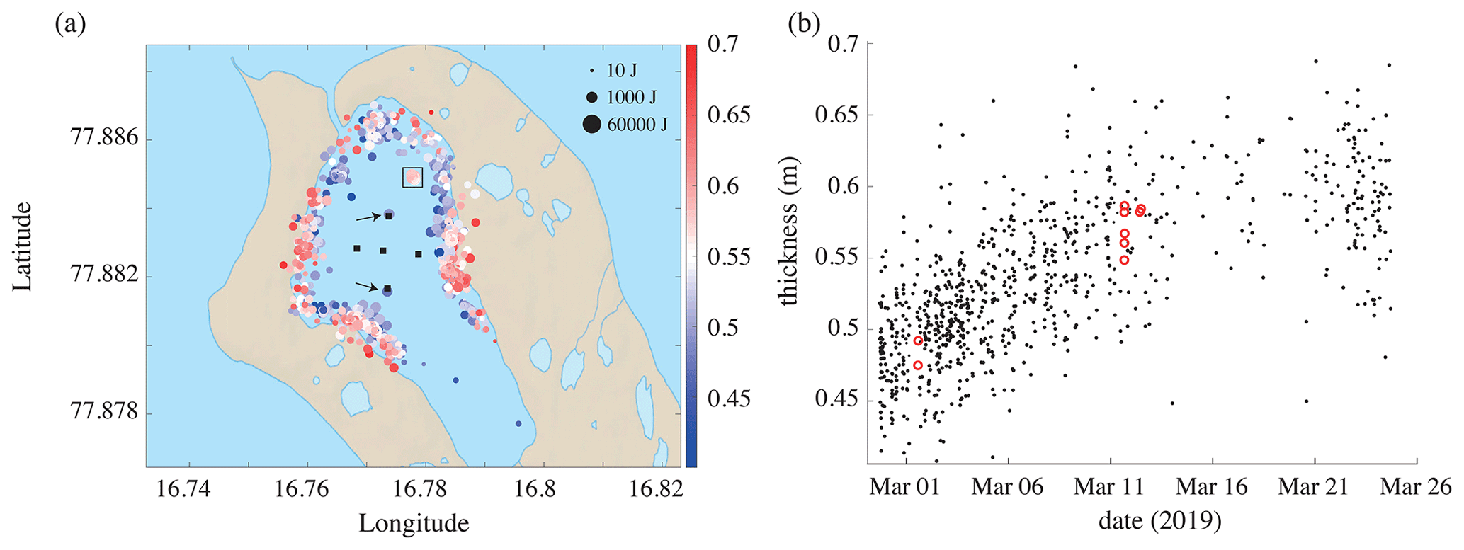
Figure 7(a) Map of the position of the inverted icequakes. The color bar indicates the corresponding ice thickness (with bounds on the thinnest and thickest values found). This thickness represents an average value along the paths between the icequake source and the five geophones. The size of the circles is proportional to the icequake energy. The black arrows indicate the position of the vertical impulsive sources, and the black square is that of the horizontal impulsive source. (b) Ice thickness versus date, obtained from icequake inversions (black dots) and from waveforms with anthropogenic sources (red circles). The squares indicate values found by drilling the ice. We note a sharp increase in thickness during the first 2 weeks of deployment, followed by a stabilization during the remaining days, which is consistent with the rise in temperatures shown in Fig. 5.
Figure 7a also shows, in color, the range of thicknesses associated with the 1790 selected inversions. Different thicknesses appear from identical positions, indicating that ice thickness has increased between the beginning and the end of the deployment. This is more visible in Fig. 7b, where the inverted thicknesses are represented versus time. On average, the thickness increased by about 15 cm, which is consistent with the increase reported in Serripierri et al. (2022), but dispersion is more significant. This is because, in the present paper, ice thickness is evaluated from all directions along the shoreline and covers a much larger range of distances from the stations (from 5 to 1000 m) than in Serripierri et al. (2022), where it is evaluated along two lines of receivers oriented north–south and east–west, with both lines having a length of 50 m. It is noteworthy that thickness estimates using only icequakes that originate from the same region and at a similar date have a significantly reduced dispersion that is consistent with the standard deviation of each individual inversion, as shown in Fig. 8.
The ice thickness increase was also confirmed by ice drillings on 1 and 25 March. There is a sharp increase in thickness during the first 2 weeks, followed by a stabilization during the remaining days. This is consistent with the temperature shown in Fig. 5, which shows variations between −15 and −30 ∘C in the first half of March, while temperatures rose between −10 and 0 ∘C in the second half.
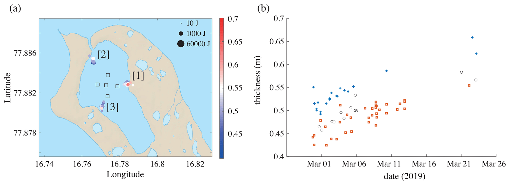
Figure 8(a) Same as Fig. 7a, restricted to icequakes originating only from directions marked as [1], [2] and [3]. (b) Same as Fig. 7b, for the icequakes in the three groups shown in Fig. 8a: + for group [1], ∘ for group [2] and □ for group [3]. Inversions originating from the same region and at a similar date have a range of thicknesses that is consistent with the standard deviation of each individual inversion (i.e., 2.5 cm). When comparing all directions, however, the range of thicknesses is on the order of 20 cm.
It is noteworthy that Fig. 7a represents all the recorded icequakes during the 27 d of geophone deployment. However, given the number of icequakes recorded every day, it could be possible to generate a similar map for each day, hence achieving near-real-time maps of sea ice thickness evolution.
3.2 Energy of the artificial sources
Estimating the energy of the icequakes requires information about the decay of amplitude between the source and the receivers due to geometrical spreading, energy leakage in water and air, and the influence of snow. This can be achieved by exploiting the waveforms from the jumps on the ice. To this end, we proceed with the following steps:
-
Isolate inversions for which the source position is closest to stations S3 and S5, where the jumps were made.
-
Calculate the corresponding energy at each geophone: , where T is the duration of the waveform and UZ, UN and UE are the vertical, northward and eastward displacement components, respectively.
-
Fit the energies versus the distance r to obtain the energy decay function Ej(r). The amplitude of a guided wave in plate-like structures can be described with Hankel functions; hence we fit the square of a Hankel function to approximate this decay.
-
Extrapolate the fitted energy decay function up to the largest distance between the icequakes and the geophones.
Jumps on the ice were performed from a height of 1 m by a person weighing 85 kg, so the kinetic energy of the jumps is about 850 J. Hence Ej(r) can be used to estimate Es(r=0), the energy of the other sources, from Es(r(Si)), the energy measured from the waveforms at geophone Si, located at a distance r(Si) from the source, such that
For example, applying this formula to the ice floe collisions, northeast of station S3 (see the black square in Fig. 7a), we are able to estimate the energy of these sources to be on the order of 40 kJ (Fig. 9a). Given the weight of the ice floe, 39 t, the speed of the floe at the impact should be of about 1.4 m s−1, which is walking speed. Of course, this approach is only a “first-order” estimation of the energy because it does not account for all the physics of the problem, such as source mechanism, source directivity and scattering. However, it provides interesting statistics about the scaling law of the icequakes in sea ice.
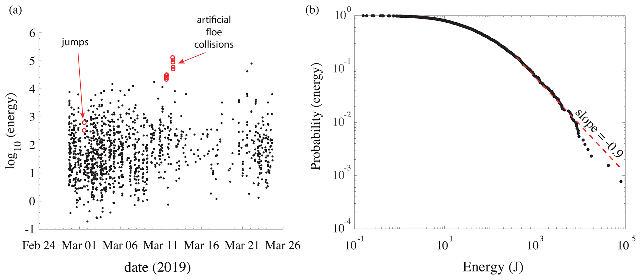
Figure 9(a) Energy versus date of all inverted icequakes (black dots) and artificial sources (red circles). (b) Scaling law of the icequake energy.
3.3 Energy of the icequakes
Here we apply Eq. (1) to calculate the energy of the 1790 icequakes selected out of the 5350 inversions. The results are shown in terms of the energy versus date in Fig. 9a and in terms of the scaling law of the energy in Fig. 9b. Energies vary between less than 1 J and about 40 kJ. By comparison with earthquakes energy, this corresponds to energy magnitudes between −3.7 and −0.2, where the conversion was obtained with the energy magnitude formula (Choy and Boatwright, 1995) of .
In the artificial ice floe collisions, the impact surface is 5 m × 0.8 m =4 m2 and causes an energy release of about 40 kJ. The average icequake energy is about 500 J, which is 2 orders of magnitude weaker. This suggests that the majority of icequakes are generated by cracks that are a few centimeters long, but there are also icequakes generated by cracks several meters long.
The scaling law of the icequakes was calculated following Clauset et al. (2009), which gave a power law with a slope of −0.9 between 400 and 80 000 J, which is validated by a Kolmogorov–Smirnov test (Massey, 1951) that gives a p value of 0.078. This is a bit larger than for earthquakes, for which the typical scaling law in terms of energy has a slope of −0.66 (see above in the Gutenberg–Richter law). However, the comparison is only indicative and serves no other goal, since very little is known about sea ice dislocation mechanisms, which are presumably quite different than those of fault zones.
The forward model used for data inversion assumes a constant ice thickness, which is not the case in reality. Our estimations of ice thickness represent an apparent value that we assume to be an average between the icequakes source and the five geophones. It is noteworthy that this assumption should not hold if the ice thickness varied monotonically. In that case, without a forward model that accounts for linear thickness variations, for example in a free plate (Moreau et al., 2014), the apparent ice thickness would be biased towards the value directly under the receivers (Romeyn et al., 2021), due to adiabatic mode propagation. However, it is very unlikely that there was a monotonic thickness increase (or decrease) at the place of the experiment, although it is not possible to verify without ground-truth values. More likely would be that there were random thickness variations of a few centimeters between the shoreline and the geophones. Nonetheless, the path between the source and each geophone is not the same, so the ice thickness is likely to be slightly different from one path to another. This is thus the reason for the assumption that the apparent thickness is an average.
This model, like all models based on plate theory, also suffers the limitation of being restricted to low frequencies. Ongoing comparisons between inversions using this model and a full numerical model based on the spectral-element method (Cao et al., 2021) suggest that using a model based on plate theory underestimates the ice thickness by a few centimeters, as soon as the frequency band of interest includes frequencies above 10 Hz, for an ice thickness of 1 m. Moreover, these numerical investigations also reveal that the snow layer, if not accounted for in the model, leads to some estimations that reflect “apparent values” for the ice thickness and mechanical properties (Moreau et al., 2020a). In particular, the snow layer introduces a gradient of porosity through the thickness which makes the flexural wave velocity lower, resulting in potential underestimation of the ice thickness.
These are, however, preliminary results, and the investigation is still ongoing. The full study will be presented in detail in a separate paper. These limitations to the model (plate theory and not accounting for snow), together with the spatial heterogeneity of the ice thickness in the field, explain why the thickness estimations appear to be slightly less that those measured by drilling the ice (Fig. 7b).
Both the abovementioned issues will be tackled in future developments by using the relocated icequakes as sources for a tomographic inversion of the thickness, for example based on full waveform inversion strategies with a spectral-element-based forward model, which also accounts for the snow layer.
Currently, we are only making use of the vertical-displacement component in this type of inversion. However, by making use of the horizontal-displacement components, it will be possible to also recover and monitor Young's modulus and Poisson's ratio, instead of using a constant value. As demonstrated in Serripierri et al. (2022), these parameters can be constrained by exploiting the waveforms of the other two guided modes, QS0 and SH0, for which polarization is on the horizontal-displacement components. This could be useful regarding drifting pack ice for long-term monitoring. In the present study, using a constant value for these parameters is, however, a valid assumption, since these have been shown to remain constant around E=3.8 GPa and ν=0.28, during the 27 d of deployment (Serripierri et al., 2022).
A particularly appealing aspect of this approach is the ability to adapt the frequency of investigation to the required spatial resolution. The wavelength of the seismic modes guided in the ice layer depends on the product of the ice thickness by the frequency. It typically varies from a few meters around 100 Hz m to a few hundred meters around 0.1 Hz m. Hence, on drifting pack ice, by adjusting the size of the geophones antenna, the spatial resolution of the maps can vary from tens of meters to a few kilometers.
The ideal monitoring conditions in the fjord allow for the development of such methodologies, in view of a transfer to the open Arctic ocean. In Moreau et al. (2020b), the inversion method was successfully applied to a few icequakes identified “manually” in continuous recordings on drifting pack ice in the Arctic. To transfer the methodology of this paper in a less favorable environment, the preferred approach is to join other scientific projects on sea ice, for example during ice camps on fast ice or on board an icebreaker. This is planned in the coming 2 or 3 years. Another possibility, dedicated to long-term monitoring, is to make use of geophones that can telemeter the continuous recordings via satellite, such as those used in Marsan et al. (2019) to record seismic noise on drifting ice floes. However, this requires a large budget, which for the most part is dedicated to the use of satellite bandwidth.
The thermomechanical processes that generate the icequakes recorded in the fjord are likely a combination of thermal fracture such as those observed in lakes (Ruzhich et al., 2009) or in glaciers (Podolskiy et al., 2019) and mechanical forcing due to tide, as observed in glaciers (Barruol et al., 2013). The 24 h periodicity of icequakes, as shown in Figs. 3 and 6, is not correlated with temperature variations, which suggests that the latter effect is dominant compared to the former. The range of energy of the recorded icequakes is consistent with that reported in frozen lakes, for example in Ruzhich et al. (2009) or Kavanaugh et al. (2018).
We conducted a systematic analysis of the microseismicity recorded on fast ice in Svalbard. The analysis consists of a two-step processing of the seismic data. First, a deep learning algorithm is used for clustering the waveforms into different families of signals: icequakes, background noise, anthropogenic noise, etc. Clusters containing thousands of icequakes were identified, from which the waveforms of the QS mode were extracted. Then, Bayesian inversion was applied to these waveforms to determine the position of the seismic sources and the average ice thickness between the sources and the geophones. Icequakes were found to originate from all along the shoreline of the fjord, where mechanical stress due to tides induces cracking, most of which occurs with a recurrence of about 24 h. Our analyses also reveal that the recorded icequakes are likely to be generated by source mechanisms that are quite different from dislocations encountered for earthquakes because the energy of the icequakes is mainly on the horizontal-displacement components, which are dominated by the SH0 and QS0 modes. However, these modes are excited by traction/compression motion, which is not compatible with the anti-symmetric motion of vertical dislocations.
The ice thickness was found to increase by about 15 cm during the first 2 weeks of deployment, which is consistent with the low temperatures in the first half of March 2019 and confirmed by ice drillings at the beginning and the end of March. Finally, using artificial impulsive sources, we were able to determine a scaling law of the icequake energy, ranging between 1 J and 30 kJ and exhibiting a log-normal distribution with slope −0.9.
In a future work, by including the waveforms of the three guided modes instead of using only that of the QS mode, it will be possible to exploit the whole content of the recordings via full waveform inversions strategies, in order to generate maps of sea ice parameters with a spatial resolution of tens of meters.
These data will also be very useful to train a deep neural network able to instantly estimate both the source position and the ice properties, without the need to go through a computationally expensive MCMC inversion, enabling the possibility of real-time in situ estimation of the ice thickness and cracks.
scatseisnet strategy The scatseisnet algorithm operates with the processing steps shown in Fig. A1. These steps are briefly detailed in this section.

Figure A1Computing scheme of the scatseisnet method. The seismograms are fed to a deep scattering network for extracting the scattering coefficients. The most relevant features are extracted from the scattering coefficients with an independent component analysis. Clusters are identified with an agglomerative-clustering technique.
A1 Deep scattering network
A scattering network is a deep convolutional neural network with wavelet filters. Although a thorough description of the deep scattering network is provided in Andén and Mallat (2014), we provide a succinct description here for self-consistency of this paper. Considering the continuous three-component input data segment u(t)∈ℝ3, the scattering coefficients S(ℓ) of order ℓ are the result of a cascade of wavelet convolutions and modulus operations, such as
where ⋆ denotes the convolution operation; is the modulus; and ϕ(i)(fi) is the wavelet filter at the layer i of the scattering network, with center frequency fi. Here fi refers to one of the center frequencies of the layer i, which is defined by the operator. While the authors in Seydoux et al. (2020) implement learnable wavelet filters ϕ(i) with respect to the clustering loss, we here directly use Gabor filters, as originally proposed in Andén and Mallat (2014) and implemented in Steinmann et al. (2022) to allow for faster computations. The maximum operator performs a pooling reduction over the time interval , allowing for reducing the complexity carried by the waveform itself. We prefer it over the low-pass filter operation originally proposed in Andén and Mallat (2014) to maximize our change to make pulse-like signals dominate the final representation.
A2 Scattering coefficients
The first wavelet transform provides a time frequency representation of the input seismic waveform – namely a scalogram – which is routinely used by seismologists. Thanks to the modulus operation, the wavelet transform represents the envelope of the input signal as a function of time in the frequency band of the wavelet filter ϕ(1)(f1) centered around the frequency f1. The second-order wavelet transforms perform a scalogram of every envelope provided by the first-order wavelet transform. This second-order transform provides information on the modulation of the signal's envelope within different frequency bands and therefore allows for discriminating signals with the same frequency content but different temporal histories. Following Andén and Mallat (2014), we use a maximum of two layers in the scattering network, provided that the third layer slightly improves auto-classification performance at a high computational cost.
A3 Independent component analysis
The number of coefficients generated by the deep scattering network is large (a few hundred), meaning that the dimension of the feature vector for every window is high-dimensional. Although the dimension is large, the information provided by the neighboring scattering coefficient is highly similar in essence (Andén and Mallat, 2014). In order to reduce the dimension, as well as inherently improve the computational performances, we extract the most relevant features with an independent component analysis (Comon, 1992), which solves the problem of factorizing the data matrix into a source matrix, and a mixing matrix under the constrain that the sources should be maximally independent.
A4 Agglomerative clustering
We finally use agglomerative clustering to identify clusters in the data. By computing the linkage matrix, we form a dendrogram (as represented in Fig. 3a). The dendrogram indicates how clusters form as a function of the merging distance. By defining an arbitrary threshold, we can obtain a varying number of clusters. For more details, please consider reading Steinmann et al. (2022).
Codes are available at
https://doi.org/10.5281/zenodo.7755633 (Moreau, 2023a).
All metadata for this experiment are available online (https://doi.org/10.15778/RESIF.XG2019; Moreau and RESIF, 2019). A subset can be accessed instantly via a direct download link. To request this link, please send an email to resif-dc@ujf-grenoble.fr with your affiliation and IP address. The full dataset (total size of 3.2 TB) is available upon request to the corresponding author, but we do not have the possibility of having such a large dataset made available with a download link. Catalogs of extracted icequakes can be downloaded at https://doi.org/10.5281/zenodo.7755650 (Moreau, 2023b).
LM designed and led the Icewaveguide (IWG) experiment in the scope of the IWG project (no. ANR10 LABX56). He supervised the manuscript preparation and the research process.
LM and JW participated in the deployment of the seismic array. LS and MC designed the scatseisnet algorithm.
The contact author has declared that none of the authors has any competing interests.
Publisher's note: Copernicus Publications remains neutral with regard to jurisdictional claims in published maps and institutional affiliations.
The Institut des Sciences de la Terre (ISTerre) is part of LABEX OSUG@2020 (grant no. ANR10 LABX56). This research was funded by the Agence Nationale de la Recherche (ANR, France) and by the Institut Polaire Français Paul-Émile Victor (IPEV).
Most of the computations presented in this paper were performed using the GRICAD infrastructure (https://gricad.univ-grenoble-alpes.fr, last access: 21 March 2023), which is supported by Grenoble research communities.
Michel Campillo and Léonard Seydoux acknowledge support from the European Research Council under the European Union Horizon 2020 research and innovation program (F-IMAGE; grant no. 742335).
Michel Campillo and Léonard Seydoux had support from the Multidisciplinary Institute in Artificial Intelligence (MIAI@Grenoble Alpes; investissements d'avenir contract no. ANR-19-P3IA-0003, France).
This research was funded by the Agence Nationale de la Recherche (grant no. ANR-17-CE01-0019), the Institut Polaire Français Paul-Emile Victor, and the European Research Council under the European Union Horizon 2020 research and innovation program (F-IMAGE; grant no. 742335).
This paper was edited by Evgeny A. Podolskiy and reviewed by Rowan Romeyn and one anonymous referee.
Andén, J. and Mallat, S.: Deep Scattering Spectrum, IEEE T. Sign. Process., 62, 4114–4128, https://doi.org/10.1109/TSP.2014.2326991, 2014. a, b, c, d, e, f
Anderson, D.: Preliminary results and review of sea ice elasticity and related studies, Transactions of the Engineering Institute of Canada, 2, 2–8, 1958. a
Ardyna, M., Babin, M., Gosselin, M., Devred, E., Rainville, L., and Tremblay, J.-É.: Recent Arctic Ocean sea ice loss triggers novel fall phytoplankton blooms, Geophys. Res. Lett., 41, 6207–6212, https://doi.org/10.1002/2014GL061047, 2014. a
Barruol, G., Cordier, E., Bascou, J., Fontaine, F. R., Legrésy, B., and Lescarmontier, L.: Tide-induced microseismicity in the Mertz glacier grounding area, East Antarctica, Geophys. Res. Lett., 40, 5412–5416, https://doi.org/10.1002/2013GL057814, 2013. a
Caline, F. and Barrault, S.: Measurements of stresses in the coastal ice on both sides of a tidal crack., in: 19th IAHR International Symposium on Ice, 6 to 11 July 2008, Vancouver, British Columbia, Canada, 2008. a
Cao, J., Brossier, R., Górszczyk, A., Métivier, L., and Virieux, J.: 3-D multiparameter full-waveform inversion for ocean-bottom seismic data using an efficient fluid–solid coupled spectral-element solver, Geophys. J. Int., 229, 671–703, 2021. a
Choy, G. L. and Boatwright, J. L.: Global patterns of radiated seismic energy and apparent stress, J. Geophys. Res.-Sol. Ea., 100, 18205–18228, https://doi.org/10.1029/95JB01969, 1995. a
Clauset, A., Shalizi, C. R., and Newman, M. E. J.: Power-Law Distributions in Empirical Data, SIAM Review, 51, 661–703, https://doi.org/10.1137/070710111, 2009. a
Comon, P.: Independent Component Analysis, in: Higher-Order Statistics, edited by: Lacoume, J.-L., 29–38, Elsevier, https://hal.archives-ouvertes.fr/hal-00346684, 1992. a, b
Crary, A. P.: Seismic studies on Fletcher's Ice Island, T-3, Eos, Transactions American Geophysical Union, 35, 293–300, https://doi.org/10.1029/TR035i002p00293, 1954. a
Dumont, D.: Marginal ice zone dynamics: history, definitions and research perspectives, Philos. T. Roy. Soc. A, 380, 20210253, https://doi.org/10.1098/rsta.2021.0253, 2022. a
Eayrs, C., Holland, D., Francis, D., Wagner, T., Kumar, R., and Li, X.: Understanding the Seasonal Cycle of Antarctic Sea Ice Extent in the Context of Longer-Term Variability, Rev. Geophy., 57, 1037–1064, https://doi.org/10.1029/2018RG000631, 2019. a
Garnier, F., Fleury, S., Garric, G., Bouffard, J., Tsamados, M., Laforge, A., Bocquet, M., Fredensborg Hansen, R. M., and Remy, F.: Advances in altimetric snow depth estimates using bi-frequency SARAL and CryoSat-2 Ka–Ku measurements, The Cryosphere, 15, 5483–5512, https://doi.org/10.5194/tc-15-5483-2021, 2021. a
Hunkins, K.: Seismic studies of sea ice, J. Geophys. Res., 65, 3459–3472, 1960. a
Kavanaugh, J., Schultz, R., Andriashek, L. D., van der Baan, M., Ghofrani, H., Atkinson, G., and Utting, D. J.: A New Year's Day icebreaker: icequakes on lakes in Alberta, Canada, Can. J. Earth Sci., 56, 183–200, https://doi.org/10.1139/cjes-2018-0196, 2018. a
Marchenko, A. V. and Morozov, E. G.: Asymmetric tide in Lake Vallunden (Spitsbergen), Nonlin. Processes Geophys., 20, 935–944, https://doi.org/10.5194/npg-20-935-2013, 2013. a, b
Marchenko, A. V., Chistyakov, P. V., Karulin, E. B., Markov, V. V., Morozov, E. G., Karulina, M. M., and Sakharov, A. N.: Field experiments on collisional interaction of floating ice blocks, in: Proceedings of the 26th International Conference on Port and Ocean Engineering under Arctic Conditions, ISSN 2077-7841, 2021. a, b, c
Marsan, D., Weiss, J., Larose, E., and Métaxian, J.-P.: Sea-ice thickness measurement based on the dispersion of ice swell, J. Acoust. Soc. Am., 131, 80–91, 2012. a
Marsan, D., Weiss, J., Moreau, L., Gimbert, F., Doble, M., Larose, E., and Grangeon, J.: Characterizing horizontally-polarized shear and infragravity vibrational modes in the Arctic sea ice cover using correlation methods, J. Acoust. Soc. Am., 145, 1600–1608, 2019. a, b
Massey, F. J.: The Kolmogorov-Smirnov Test for Goodness of Fit, J. Am. Stat. A., 46, 68–78, 1951. a
Mayot, N., Matrai, P. A., Arjona, A., Bélanger, S., Marchese, C., Jaegler, T., Ardyna, M., and Steele, M.: Springtime Export of Arctic Sea Ice Influences Phytoplankton Production in the Greenland Sea, J. Geophys. Res.-Oceans, 125, e2019JC015799, https://doi.org/10.1029/2019JC015799, 2020. a
Moreau, L.: Python package for icequakes inversions (Version 1), Zenodo [code], https://doi.org/10.5281/zenodo.7755633, 2023a. a
Moreau, L.: Catalog of icequakes recorded in March 2019, in the Van Mijen Fjord, in Svalbard (Norway), Zenodo [data set], https://doi.org/10.5281/zenodo.7755650, 2023b. a
Moreau, L. and RESIF: Svalbard – Vallunden (Icewaveguide) (RESIF – SISMOB_Nodes), RESIF – Réseau Sismologique et géodésique Français [data set], https://doi.org/10.15778/resif.xg2019, 2019. a, b
Moreau, L., Minonzio, J.-G., Talmant, M., and Laugier, P.: Measuring the wavenumber of guided modes in waveguides with linearly varying thickness, J. Acoust. Soc. Am., 135, 2614–2624, 2014. a
Moreau, L., Lachaud, C., Théry, R., Predoi, M. V., Marsan, D., Larose, E., Weiss, J., and Montagnat, M.: Monitoring ice thickness and elastic properties from the measurement of leaky guided waves: A laboratory experiment, J. Acoust. Soc. Am., 142, 2873–2880, 2017. a
Moreau, L., Boué, P., Serripierri, A., Weiss, J., Hollis, D., Pondaven, I., Vial, B., Garambois, S., Larose, É.,Helmstetter, A., Stehly, L., Hillers, G., and Gilbert, O.: Sea ice thickness and elastic properties from the analysis of multimodal guided wave propagation measured with a passive seismic array, J. Geophys. Res.-Oceans, 125, e2019JC015709, https://doi.org/10.1029/2019JC015709, 2020a. a, b, c, d, e, f
Moreau, L., Weiss, J., and Marsan, D.: Accurate estimations of sea-ice thickness and elastic properties from seismic noise recorded with a minimal number of geophones: from thin landfast ice to thick pack ice, J. Geophys. Res.-Oceans, 125, e2020JC016492, https://doi.org/10.1029/2020JC016492, 2020b. a, b, c, d, e, f
Olinger, S. D., Lipovsky, B. P., Wiens, D. A., Aster, R. C., Bromirski, P. D., Chen, Z., Gerstoft, P., Nyblade, A. A., and Stephen, R. A.: Tidal and Thermal Stresses Drive Seismicity Along a Major Ross Ice Shelf Rift, Geophys. Res. Lett., 46, 6644–6652, https://doi.org/10.1029/2019GL082842, 2019. a
Parkinson, C. L.: A 40-y record reveals gradual Antarctic sea ice increases followed by decreases at rates far exceeding the rates seen in the Arctic, P. Natl. Acad. Sci. USA, 116, 14414–14423, https://doi.org/10.1073/pnas.1906556116, 2019. a
Podolskiy, E. A., Fujita, K., Sunako, S., and Sato, Y.: Viscoelastic Modeling of Nocturnal Thermal Fracturing in a Himalayan Debris-Covered Glacier, J. Geophys. Res.-Earth Surf., 124, 1485–1515, https://doi.org/10.1029/2018JF004848, 2019. a
Romeyn, R., Hanssen, A., Ruud, B. O., and Johansen, T. A.: Sea ice thickness from air-coupled flexural waves, The Cryosphere, 15, 2939–2955, https://doi.org/10.5194/tc-15-2939-2021, 2021. a, b, c
Ruzhich, V., Psakhie, S., Chernykh, E., Bornyakov, S., and Granin, N.: Deformation and seismic effects in the ice cover of Lake Baikal, Russ. Geol. Geophys.+, 50, 214–221, https://doi.org/10.1016/j.rgg.2008.08.005, 2009. a, b
Sabra, K. G., Gerstoft, P., Roux, P., Kuperman, W., and Fehler, M. C.: Extracting time-domain Green's function estimates from ambient seismic noise, Geophys. Res. Lett., 32, L03310, https://doi.org/10.1029/2004GL021862, 2005. a
Serripierri, A., Moreau, L., Boue, P., Weiss, J., and Roux, P.: Recovering and monitoring the thickness, density, and elastic properties of sea ice from seismic noise recorded in Svalbard, The Cryosphere, 16, 2527–2543, https://doi.org/10.5194/tc-16-2527-2022, 2022. a, b, c, d, e, f
Seydoux, L., Balestriero, R., Poli, P., Hoop, M. d., Campillo, M., and Baraniuk, R.: Clustering earthquake signals and background noises in continuous seismic data with unsupervised deep learning, Nat. Commun., 11, 3972, https://doi.org/10.1038/s41467-020-17841-x, 2020. a, b, c
Shapiro, N. M. and Campillo, M.: Emergence of broadband Rayleigh waves from correlations of the ambient seismic noise, Geophys. Res. Lett., 31, L07614, https://doi.org/10.1029/2004GL019491, 2004. a
Stein, P. J., Euerle, S. E., and Parinella, J. C.: Inversion of pack ice elastic wave data to obtain ice physical properties, J. Geophys. Res.-Oceans, 103, 21783–21793, 1998. a, b
Steinmann, R., Seydoux, L., Beaucé, É., and Campillo, M.: Hierarchical Exploration of Continuous Seismograms With Unsupervised Learning, J. Geophys. Res.-Sol. Ea., 127, e2021JB022455, https://doi.org/10.1029/2021JB022455, 2022. a, b, c
Yang, T. and Giellis, G.: Experimental characterization of elastic waves in a floating ice sheet, J. Acoust. Soc. Am., 96, 2993–3009, 1994. a