Sea ice classification of TerraSAR-X ScanSAR images for the MOSAiC expedition incorporating per-class incidence angle dependency of image texture

We provide sea ice classification maps of a sub-weekly time series of single (horizontal–horizontal, HH) polarization X-band TerraSAR-X scanning synthetic aperture radar (TSX SC) images from November 2019 to March 2020, covering the Multidisciplinary drifting Observatory for the Study of Arctic Climate (MOSAiC) expedition. This classified time series benefits from the wide spatial coverage and relatively high spatial resolution of TSX SC data and is a useful basic dataset for future MOSAiC studies on physical sea ice processes and ocean and climate modeling. Sea ice is classified into leads, young ice with different backscatter intensities, and first-year ice (FYI) or multiyear ice (MYI) with different degrees of deformation. We establish the per-class incidence angle (IA) dependencies of TSX SC intensities and gray-level co-occurrence matrix (GLCM) textures and use a classifier that corrects for the class-specific decreasing backscatter with increasing IAs, with both HH intensities and textures as input features. Optimal parameters for texture calculation are derived to achieve good class separation while maintaining maximum spatial detail and minimizing textural collinearity. Class probabilities yielded by the classifier are adjusted by Markov random field contextual smoothing to produce classification results. The texture-based classification process yields an average overall accuracy of 83.70 % and good correspondence to geometric ice surface roughness derived from in situ ice thickness measurements (correspondence consistently close to or higher than 80 %). A positive logarithmic relationship is found between geometric ice surface roughness and TSX SC HH backscatter intensity, similar to previous C- and L-band studies. Areal fractions of classes representing ice openings (leads and young ice) show prominent increases in middle to late November 2019 and March 2020, corresponding well to ice-opening time series derived from in situ data in this study and those derived from satellite synthetic aperture radar (SAR) and optical data in other MOSAiC studies.

1 Introduction

During the 1-year-long Multidisciplinary drifting Observatory for the Study of Arctic Climate (MOSAiC) expedition from 2019 to 2020, the icebreaker RV Polarstern drifted with sea ice along the Transpolar Drift in the central Arctic Ocean, conducting the largest multidisciplinary Arctic research expedition in history (Nicolaus et al., 2022). Satellite data acquisitions from multiple platforms were coordinated to survey the sea ice area surrounding the expedition, enabling continuous, large-scale sea ice monitoring along the drift. Moreover, extensive on-ice, airborne, and ship-based in situ data were collected surrounding the MOSAiC ice floe, where RV Polarstern was moored and the Central Observatory (CO) was established. These include data from sources such as meteorological stations, airborne laser surveys, ship radar measurements, and a distributed network of autonomous buoys (Krumpen and Sokolov, 2020; Nicolaus et al., 2021; Shupe et al., 2022). This expedition aimed to facilitate physical, biogeochemical, and ecological studies of the region, enabling multiscale quantification of relevant processes and feedbacks and, eventually, the production of improved climate and Earth system models (Krumpen et al., 2021; Nicolaus et al., 2021; Shupe et al., 2022).

Sea-ice-type classification is an important basic representation of sea ice conditions that supports various further analyses, such as the monitoring of ice breakup and lead formation, inferring the occurrence of sea ice deformation and studying ice-associated and under-ice ecology, as well as input to ocean and climate models. Satellite synthetic aperture radar (SAR) data have been widely used for sea ice classification for operational and scientific purposes due to their high spatial resolution as well as their weather- and illumination-independent monitoring capabilities (Zakhvatkina et al., 2019). Coordinated acquisitions of TerraSAR-X scanning synthetic aperture radar (TSX SC) data were conducted to provide consistent coverage of the MOSAiC ice floe throughout the expedition. This dataset provides daily X-band (9.65 GHz) imaging with an 8.25 m nominal pixel spacing, which is considerably higher than publicly available scanning synthetic aperture radar (ScanSAR) products, e.g., Sentinel-1 (S1). The extent of TSX SC scenes is approximately 100 km ×150 km. These features make TSX SC a valuable data source for detailed examinations of sea ice development for large areas around the MOSAiC ice floe. This study aims to produce a classified winter (November 2019 to March 2020) TSX SC time series surrounding the CO, which can serve as a basis for further MOSAiC sea ice studies and modeling efforts.

TSX SC scenes in this time series cover a wide range of incidence angles (IAs). Therefore, appropriate adjustment for the IA effect of the SAR signal, i.e., generally decreasing backscatter intensities with the IA, is crucial for reliable and consistent classification. The magnitude of the IA effect varies with ice type (Mäkynen et al., 2002; Mäkynen and Karvonen, 2017; Mahmud et al., 2018), which necessitates per-class IA correction. A sea ice classifier that specifically considers this phenomenon is used in this study. Developed and published by Lohse et al. (2020), this classifier directly incorporates per-class IA dependencies into a Bayesian classifier, treating the IA dependence as a class property. This classifier replaces the constant mean vector of the Gaussian probability density function with a linearly variable mean, which represents class-specific IA dependencies (Lohse et al., 2020), and is therefore named the Gaussian incidence angle (GIA) classifier. It has been developed based on S1 Extra Wide (EW) swath data and has also been used with the RADARSAT-2 (RS2) ScanSAR Wide (SCW) and Fine resolution Quad-polarization beam (FQ) data products with minor adjustments (Guo et al., 2022). The GIA classifier reliably corrects the IA effect on the HH (horizontal–horizontal) and HV (horizontal–vertical) channels of these datasets, resulting in improved classification results compared with classification with global IA correction.

TSX SC data collected for MOSAiC are in HH polarization. The same ice types can have vastly different HH intensities due to factors such as different surface characteristics, e.g., different degrees of deformation on first-year ice (FYI) and multiyear ice (MYI), and different surface roughness and salinity levels on young ice. On the other hand, some ice types have similar X-band HH intensities, e.g., MYI, deformed FYI, and young ice (e.g., Liu et al., 2016). Therefore, in addition to HH intensities, we use image textures as input to the classification to expand the feature space. Specifically, we use texture measures calculated on the basis of the gray-level co-occurrence matrix (GLCM; Haralick et al., 1973). The GLCM tabulates how different combinations of gray levels co-occur in image windows, based on which statistical measures are derived to represent the spatial variability surrounding the central pixel. GLCM textures are among the most powerful texture discrimination tools (Barber and LeDrew, 1991; Zakhvatkina et al., 2019); they have been generally widely used for the texture-based classification of remote sensing images (Hall-Beyer, 2017) and have been specifically used for the sea ice classification of X- and C-band SAR data (e.g., Clausi and Yu, 2004; Leigh et al., 2014; Zakhvatkina et al., 2017; Murashkin et al., 2018; Park et al., 2020; Lohse et al., 2021; and those publications listed in Table 1). Compared with classification based only on SAR intensities, they provide additional separability between FYI and MYI, young ice and MYI, and level and deformed ice (e.g., Holmes et al., 1984; Shokr, 1991; Leigh et al., 2014; Zakhvatkina et al., 2017; Lohse et al., 2021).

Table 1 shows the GLCM texture parameters employed in previous sea ice classification studies using X-band SAR. Texture names and parameters can be found in Haralick et al. (1973) and Conners and Harlow (1980), and they are introduced in more detail in Sect. 2.3. Table 1 presents a wide variety of datasets and parameters, indicating that various GLCM textures on different geographical scales are useful for discriminating between sea ice classes. Many studies use a limited number of texture measures and do not involve a process of selecting texture combinations based on class separability and textural collinearity.

Holmes et al. (1984)Barber and LeDrew (1991)Shokr (1991)Liu et al. (2016)Ressel et al. (2015)Zhang et al. (2019)Liu et al. (2021)

Table 1 Texture parameter selection in previous studies of X-band synthetic aperture radar (SAR) sea ice classification.

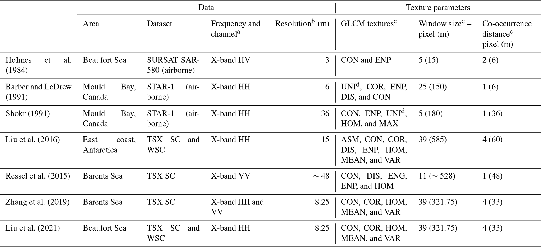
^a Only SAR channels used for GLCM calculation are shown. ^b Effective pixel spacing after preprocessing. ^c GLCM textures, window sizes, and co-occurrence distances are those used for texture-based classification or those that yield the best classification results in studies comparing different parameter combinations. ^d UNI denotes uniformity and is calculated as uniformity $={\sum }_i{\sum }_j{P}_{i,j}^{\mathrm{2}}$; therefore, it is similar to energy (ENG). Other previously undefined abbreviations and acronyms used in the table are as follows: SURSAT – SURveillance SATellite, STAR-1 – Sea Ice and Terrain Assessment Radar-1, CON – contrast, ENP – entropy, COR – correlation, DIS – dissimilarity, HOM – homogeneity, MAX – maximum probability, ASM – angular second moment, MEAN – mean, and VAR – variance.

In the logarithmic (decibel, dB) domain, S1 EW textures of the HH channel for different ice types generally have a linear relationship with IA and have been used for sea ice classification (Lohse et al., 2021). For TSX data, Ressel et al. (2015) used five GLCM textures from the VV (vertical–vertical) channel of three TSX SC images to classify sea ice near Svalbard with an artificial neural network (ANN) and reported satisfactory results for scenes with similar IA ranges to the training scene. Liu et al. (2016) used eight GLCM textures from TSX SC and Wide ScanSAR (WSC) data to classify sea ice on the east coast of Antarctica, using IA directly as an input feature to a support vector machine (SVM) classifier. Zhang et al. (2019) used five GLCM textures in an SVM classifier on five TSX SC (HH and VV) scenes, and Liu et al. (2021) used the same five GLCM textures on eight TSX SC and WSC (HH) scenes to classify sea ice, both in the Beaufort Sea, with no corrections for the IA effect. To our knowledge, no previous study has demonstrated the IA dependencies of different Arctic sea ice types for TSX SC intensities and GLCM textures.

This study examines this phenomenon in winter during the MOSAiC campaign and, accordingly, includes GLCM textures as input features to the GIA classifier. Optimal parameters for texture calculation are derived to provide statistical separability between class distributions evaluated by the Kolmogorov–Smirnov (K–S) distance (Massey, 1951). A total of 17 GLCM texture measures are analyzed, which can be derived using commonly available software tools, i.e., the Sentinel Application Platform (SNAP), provided by the European Space Agency (ESA; European Space Agency, 2020), and the Google Earth Engine (GEE; Gorelick et al., 2017). As we aim to fully utilize the spatial resolution of TSX SC data, a rating system is developed to find the set of texture measures that provides class separability at the smallest window size while minimizing intercorrelations between textures.

In summary, the objectives of this study are as follows: (1) to use the GIA classifier on TSX SC HH intensity and textures to produce a classified winter time series for sea ice surrounding the area covered during the MOSAiC expedition and (2) to demonstrate per-class IA dependencies of TSX SC HH intensity and textures for the abovementioned study area and period.

2 Materials and methods

2.1 Data

This study analyzes 53 TSX SC scenes (1 November 2019 to 11 April 2020; IA from 17.18 to 59.56^∘) with an average of 3 scenes per week. All scenes are radiometrically corrected and calibrated to σ⁰ and converted to decibels. Figure 1a shows the scene boundaries for each month using black rectangles. Figure 1c shows the IA ranges of the scenes in red.

Among the aforementioned scenes, 50 scenes (1 November 2019 to 28 March 2020; IA from 31.90 to 59.56^∘) are used for sea ice classification and are hereafter referred to as the time series. The remaining three scenes (31 March 2020, 3 April 2020, and 11 April 2020; IA from 17.18 to 36.70^∘) are only included to cover the full IA range of the TSX SC data in order to examine the IA dependencies of HH intensities. They were captured at low IAs (Fig. 1c) to retain the CO, which was drifting below 85.5^∘ N (Fig. 1b), in the scene frames. These scenes exhibit consistent IA dependency with other scenes for HH intensities but not for HH textures (not shown). The spatial details obtainable from these scenes are different from others after being subjected to identical preprocessing steps, resulting in considerably different texture values. Moreover, these scenes are generally more affected by noise (Fritz et al., 2013).

We use 13 scenes, including the 3 scenes with low IAs, as reference scenes (dates and IA ranges are shown in Fig. 1c and d), from which reference polygons are derived to examine IA dependencies. These scenes are selected to cover each month between November 2019 and April 2020 as well as the full IA range of the TSX SC data. As mentioned above, the 3 scenes with low IAs are only used to demonstrate IA dependencies of HH intensities, and the other 10 reference scenes before 31 March 2020 are used to demonstrate IA dependencies of both HH intensities and textures as well as for classification training and testing.

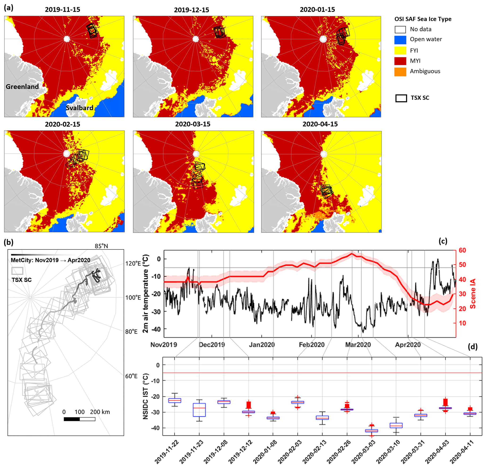
Figure 1 (a) TSX SC scenes for each month and OSI SAF sea ice classifications of surrounding sea ice areas in the middle of each month; (b) the drift track of the MetCity weather station and its position relative to TSX SC scenes; (c) 2 m air temperature records and IA ranges of TSX scenes (average IAs are shown using the red line), with vertical lines representing selected reference scenes; and (d) box plots of the NSIDC IST data within each reference scene, where boxes cover the 25th to the 75th percentile, the median is shown using the red bar, whiskers extend to data extremes excluding outliers, and red crosses indicate outliers.

Environmental conditions associated with the scenes are inferred from 2 m air temperature records from the MetCity weather station in the CO (Fig. 1c, black), the drift track of which is shown in Fig. 1b (gray line). Figure 1c shows that temperatures are mostly below −5 ^∘C during the study period except for in late April, when warm spells brought temperatures to near 0 ^∘C. For the reference scenes, near-coincident scenes (within 3 h of TSX acquisition) from the National Snow and Ice Data Center (NSIDC) MOD29/MYD29 sea ice surface temperature (IST) dataset (Hall and Riggs, 2021) are extracted to show that temperatures within TSX scene boundaries are well below −5^∘ (Fig. 1d). Overlapping S1 EW and RS2 FQ scenes and the Ocean and Sea Ice Satellite Application Facility (OSI SAF) sea ice type (OSI-403-d; Fig. 1a) product (OSI SAF, 2019) are used as qualitative visual references to aid the derivation of reference polygons, providing general knowledge about large-scale ice conditions and comparison with C-band SAR signals, respectively.

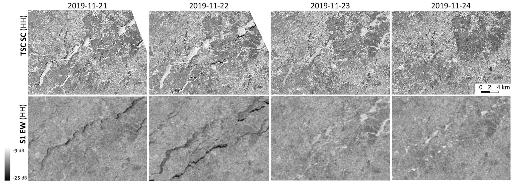
Figure 2 Progression of young ice on near-coincident TSX SC and S1 EW scenes scaled by the same range of intensities. All subsequent figures of HH intensities use the decibel range shown here.

Young ice shows a wide range of HH intensities due to differences in surface characteristics; this affects ice-type classification. Figure 2 shows an example of the progression of young ice on overlapping TSX SC and S1 EW scenes in HH polarization. On 20 November 2019, widespread lead openings occurred around the CO. Between 20 and 21 November 2019, more openings appeared that quickly refroze into young ice. On the TSX scenes from 21 November 2019, most of the young-ice areas appear very bright. Subsequently, young ice gradually darkens to brightness levels similar to the surrounding ice. On the S1 scenes, the HH intensities of young ice gradually increase from brightness levels similar to or lower than the nearby ice to very bright on 23 and 24 November 2019. Afterwards, they again darken to a similar brightness level to their surroundings. The changing young-ice intensities are presumably due to evolving surface roughness, e.g., influenced by the formation and evolution of frost flowers, which are highly saline and have different sizes, leading to varying scales of surface roughness (Martin et al., 1995; Barber et al., 2014; Isleifson et al., 2018; Johansson et al., 2018). The delayed increase and decrease in young-ice backscatter in the C band (5.405 GHz) compared with the X band (9.65 GHz) are then presumably due to different interactions between changing surface roughness scales and different SAR wavelengths (Isleifson et al., 2010; Dierking, 2010; Barber et al., 2014; Park et al., 2020). These observations confirm the need to split young ice into separate classes for ice-type classification, as described below.

2.2 Reference polygons of sea ice classes

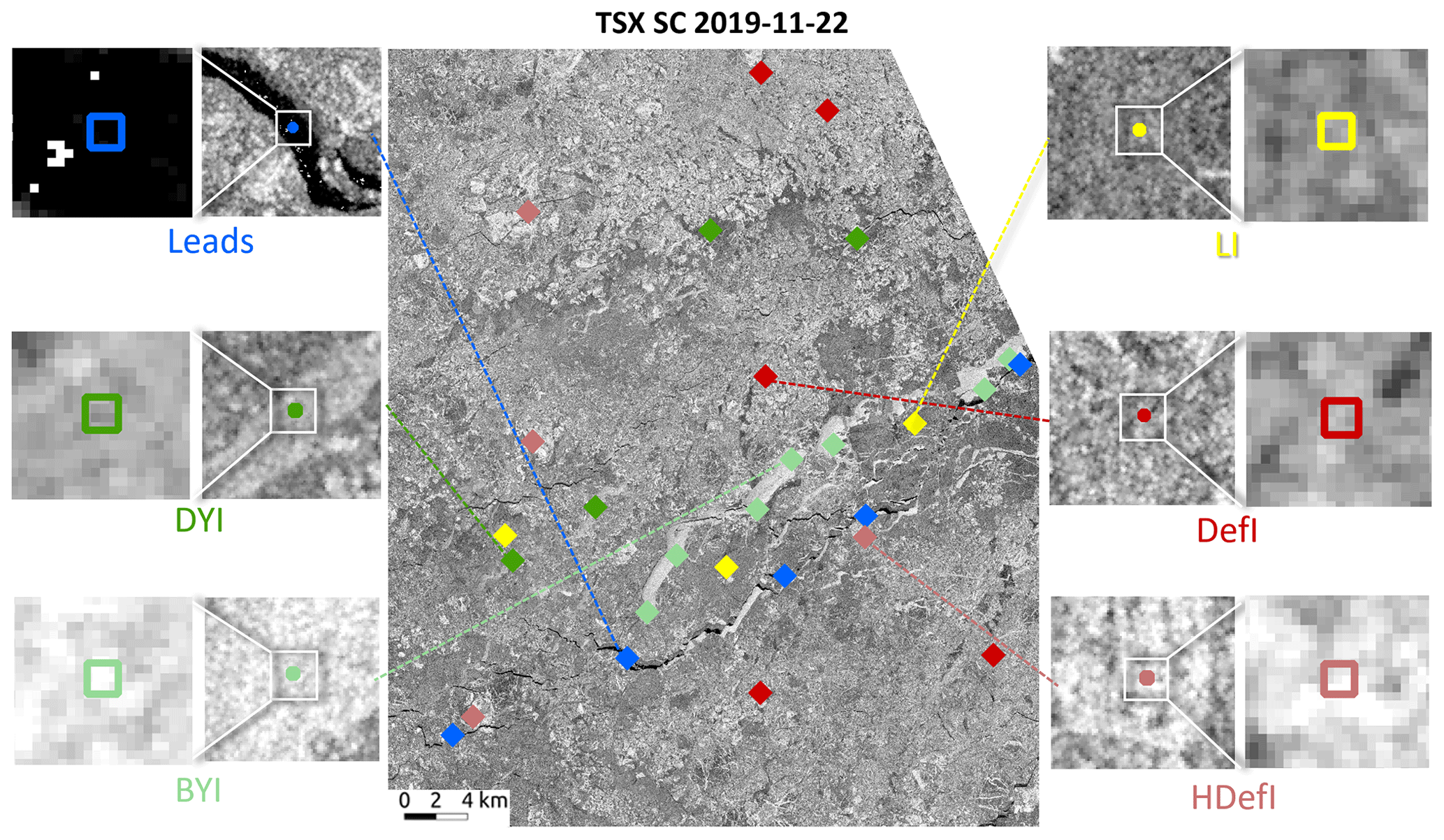
Based on the ice conditions in the study area and period, we classify sea ice into leads, rough young ice with different HH intensities, and FYI or MYI with different deformation states. The intensity thresholds shown below are empirically derived approximate values only used as one of the criteria in deriving the reference polygons. These classification thresholds are defined as follows:

Figure 3 Example reference polygons of different classes over the scene on 22 November 2019.

1. Leads are ice openings occupied by calm open water, nilas, or smooth newly formed ice and have the lowest HH intensities ($<-\mathrm{25}$ dB). Separation in open water due to different wind states is not within the scope of this study, and a visual examination shows that open-water leads in the time series are all narrow (≤250 m) and predominantly occur in a calm state.

2. Dark young ice (DYI) refers to newly formed ice in leads and has relatively high HH intensities ($\ge -\mathrm{15}$ dB), irrespective of thickness. Young ice is further split into two classes, as mentioned above, with the DYI class having comparatively low intensities (between −15 and −10 dB). The separated young-ice classes do not correspond to existing ice types in the World Meteorological Organization (WMO) nomenclature (WMO, 2018).

3. Bright young ice (BYI) denotes rough young ice with HH intensities of greater than −10 dB.

4. Level ice (LI) refers to smooth FYI or MYI areas with intermediate HH intensities that are between those of leads and DYI (−25 and −15 dB, respectively).

5. Deformed ice (DefI) is rough FYI or MYI with HH intensities between −15 and −10 dB.

6. Heavily deformed ice (HDefI) refers to FYI or MYI areas with very high degrees of deformation and, thus, high HH intensities ($\ge -\mathrm{10}$ dB).

For each class, 15 reference polygons in 3 pixel ×3 pixel rectangles are manually derived for each reference scene to standardize the number of reference pixels between classes. The polygon size is determined to accommodate typical widths of small or linear surface features, i.e., classes representing “lead ice” (leads, DYI, and BYI) and HDefI. The former usually takes a linear shape along ice openings, and the latter usually includes (1) linear strips or spatially limited aggregations of deformation features or (2) rounded MYI floes. Therefore, polygons are placed at the center of small, rounded features and along the width of linear features. To minimize spatial dependence, a minimum distance of 50 pixels is maintained between polygons, and polygons for each class are distributed evenly across the scenes where possible. Polygons of each class in each scene are then randomly split in half for training and testing. To improve training consistency across scenes, polygons of LI, DefI, and HDefI are derived for approximately the “same ice” for all reference scenes, where possible. Figure 3 shows example reference polygons derived for 22 November 2019.

2.3 The IA dependencies of HH intensities and textures

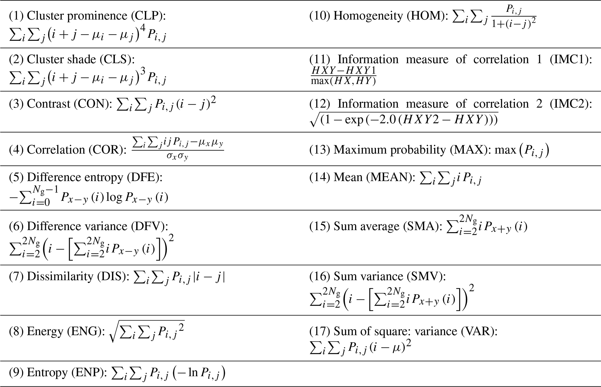
We examine IA dependencies of HH intensities and 17 GLCM textures for different ice types and evaluate class separability provided by them. This enables us to optimize the utilization of GLCM textures as classification features and classify sea ice for MOSAiC with reliable IA correction. The textures used are listed in Table 2, where the mathematical expressions match those from Haralick et al. (1973) and Conners and Harlow (1980).

Table 2 GLCM texture measures analyzed in this study, where P_i,j is the (i,j)th entry in the GLCM; ∑_i is ${\sum }_{i=\mathrm{1}}^{N_{\mathrm{g}}}$; ∑_j is ${\sum }_{j=\mathrm{1}}^{N_{\mathrm{g}}}$; N_g is the number of distinct gray levels in the quantized image; $P_{x+y}\left(k\right)={\sum }_{i=\mathrm{1}}^{N_{\mathrm{g}}}{\sum }_{j=\mathrm{1}}^{N_{\mathrm{g}}}{P}_{i,j}$ ($i+j=k;k=\mathrm{2},\mathrm{3},\mathrm{\dots },\mathrm{2}{N}_{\mathrm{g}}$); $P_{x-y}\left(k\right)={\sum }_{i=\mathrm{1}}^{N_{\mathrm{g}}}{\sum }_{j=\mathrm{1}}^{N_{\mathrm{g}}}{P}_{i,j}$ ($|i-j|=k;k=\mathrm{0},\mathrm{1},\mathrm{\dots },N_{\mathrm{g}}-\mathrm{1}$); $P_x\left(i\right)={\sum }_{j=\mathrm{1}}^{N_{\mathrm{g}}}{P}_{i,j}$; $P_y\left(j\right)={\sum }_{i=\mathrm{1}}^{N_{\mathrm{g}}}{P}_{i,j}$; μ_x, μ_y, σ_x, and σ_y are the means and standard deviations of P_x and P_y; $HXY=-{\sum }_i{\sum }_j{P}_{i,j}\log P_{i,j}$; $HXY\mathrm{1}=-{\sum }_i{\sum }_j{P}_{i,j}\log p_x\left(i\right)p_y\left(j\right)$; $HXY\mathrm{2}=-{\sum }_i{\sum }_j{p}_x\left(i\right)p_y\left(j\right)\log p_x\left(i\right)p_y\left(j\right)$; and HX and HY are the entropy of P_x and P_y, respectively.

In an initial examination of GLCM textures, we found that only textures of HH intensities in the logarithmic (dB) domain have a consistent linear relationship with IA, given a properly constrained IA range (more detail below), whereas textures of HH intensities in the linear domain do not. This linear dependency is one of the prerequisites for input features of the GIA classifier. Similar findings are reported in Lohse et al. (2021) for C-band S1 EW data. Thus, GLCM textures are calculated for HH intensities in decibels, split into 64 gray levels to achieve balance between the precision of gray-level information and computational efficiency, and averaged for four directions (0, 45, 90, and 135^∘) to avoid directional sensitivity of textures. We use a data-driven approach to optimize the other three texture parameters for image classification: co-occurrence distance, texture window size, and the combination of texture measures (more detail given in Sect. 2.4). These texture parameters are explained in Haralick et al. (1973).

The statistical distribution and scatterplots of HH intensities of the 13 reference scenes (Fig. 4) show that ambiguities in HH intensities are most prominent for two class pairs: BYI vs. HDefI and DYI vs. DefI. Thus, these difficult class pairs are the focus of subsequent separability evaluations. The IA dependency of leads is the weakest and is statistically insignificant (Fig. 4), with HH intensities mostly under the nominal noise floor (Fritz et al., 2013) and with the widest scatter. HH intensities of the other classes are generally linear with IA throughout the IA range and have significant slopes.

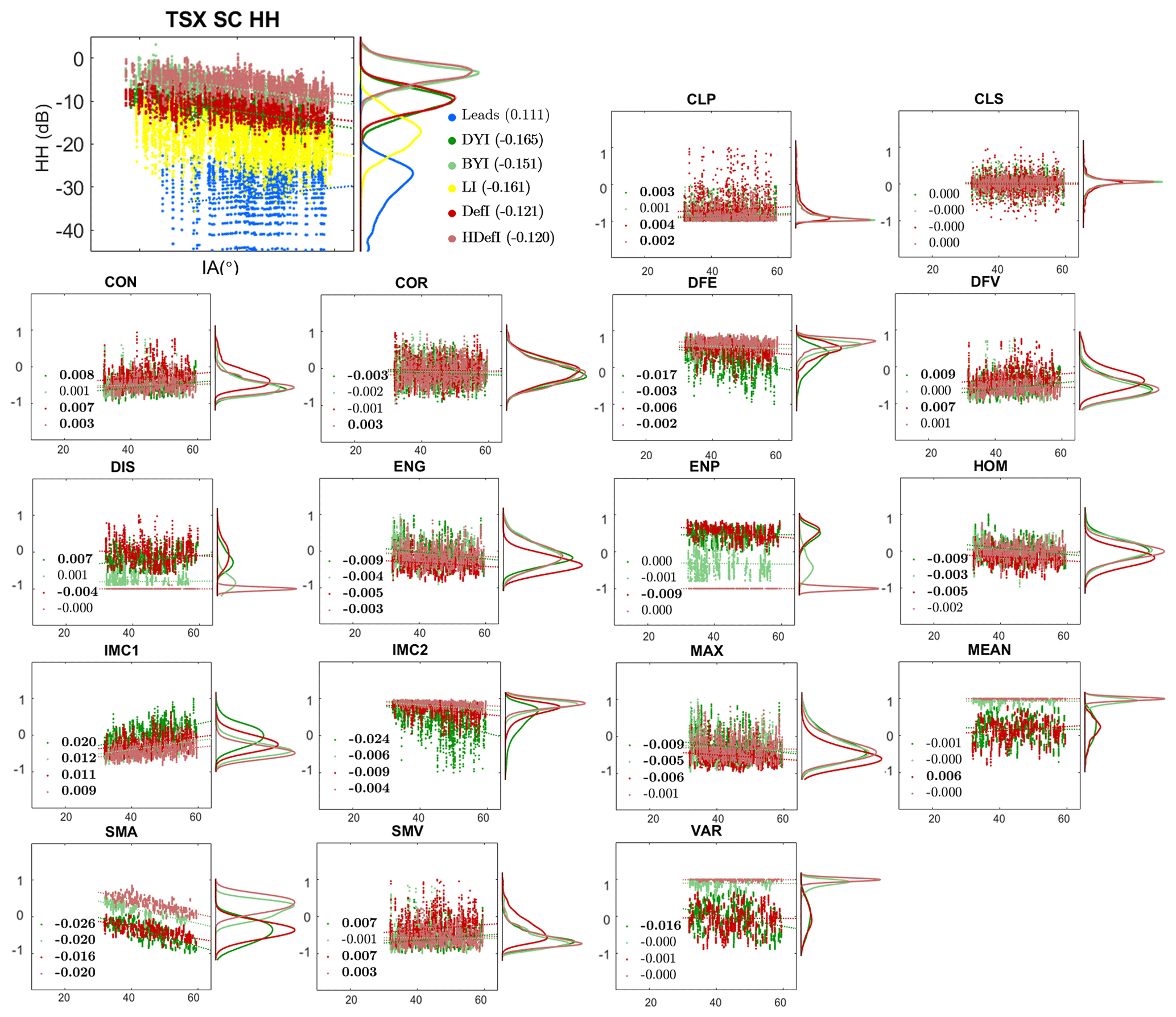
Figure 4 Histograms and scatterplots of TSX SC HH intensities with the IA for the reference polygons (all classes) and of GLCM textures (Table 2) with the IA for the training polygons (difficult class pairs). Slope values of different classes with the IA are also shown, with bold font indicating statistical significance. Values of all texture measures are scaled to the −1 to 1 range in order to yield comparable slope values.

The distribution of GLCM textures in an example window size of 9 pixels and their scatterplots in the IA range of the 10 training scenes (31.90 to 59.56^∘) are shown in Fig. 4. Only the difficult class pairs are shown for visual clarity. Textures generally show a weak linear relationship with IA with varying levels of dependencies (IA slopes), similar to previous C-band and X-band findings (e.g., Liu et al., 2016; Lohse et al., 2021; Scharien and Nasonova, 2020). Some textures show visually apparent separability between one or both of the difficult class pairs (e.g., DIS, ENP, MEAN, SMA, and VAR). The classes form approximately Gaussian distributions for HH intensities and most textures (Fig. 4), satisfying the prerequisite for input features of the GIA classifier.

A considerable part of the leads class is below the nominal noise floor, affecting its distribution for HH intensities and textures. Moreover, the leads class has distinctly different HH intensities than other classes. Therefore, the leads class is excluded from subsequent texture-based classification. A separate classification is run using HH intensities only, from which leads are extracted and used for the final classification result, which we found to provide satisfactory lead separation.

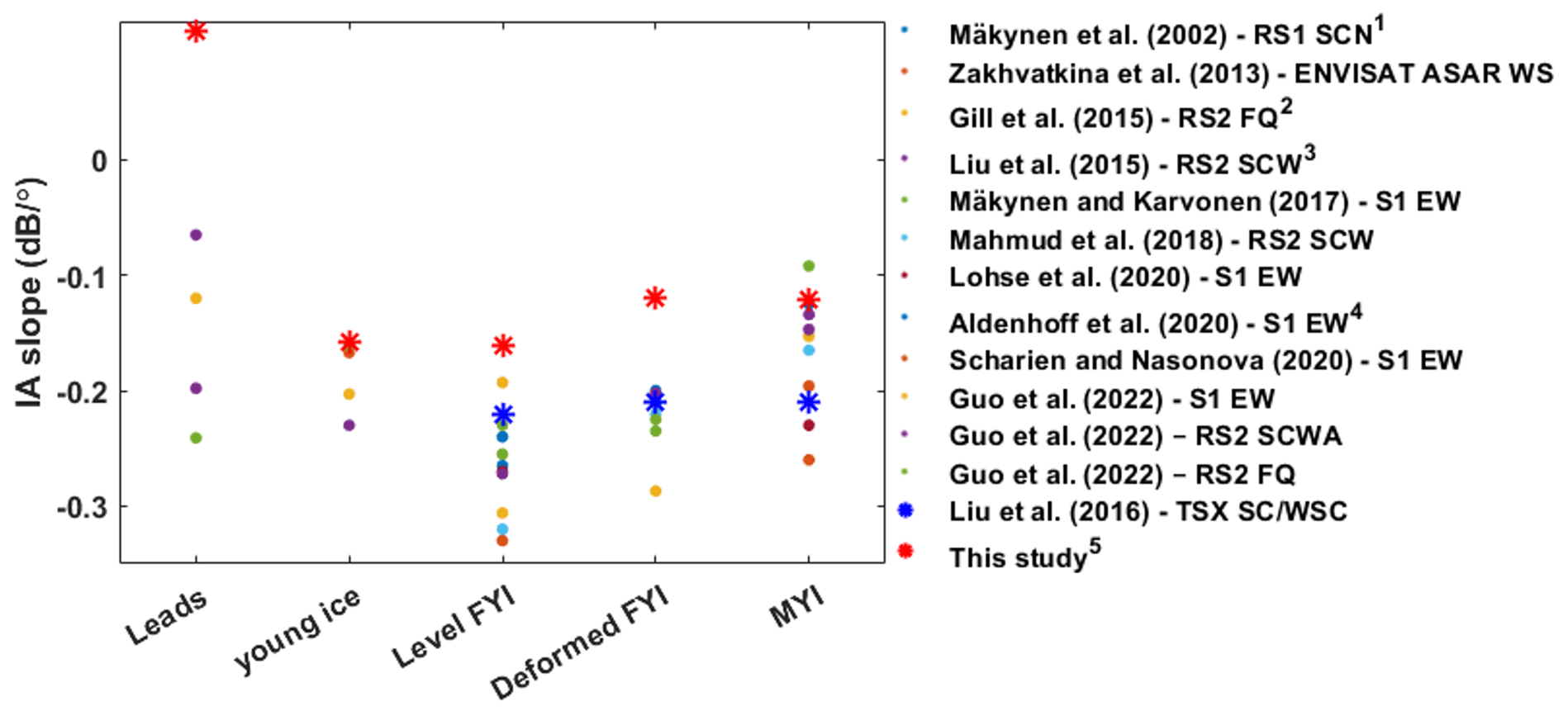
Figure 5 Comparison between IA slope values derived in this work and those from previous studies. Different classification schemes are used for these studies; we summarize these classification schemes into five commonly used classes and display per-class IA slopes for the classes that are the most closely related to these five classes. Dots denote C-band results and asterisks denote X-band results. The correspondence between ice classes shown in the figure and the closest ice classes in the original studies defined differently or more specifically is as follows (see the superscript numbers in the legend): (1) FYI – FYI with dry snow on top; (2) FYI – land-fast smooth FYI with thin (7.7±3.9 cm) to thick (36.4±12.3 cm) snow cover; (3) leads – nilas; young ice (YI) – deformed gray ice; (4) MYI – averaged for MYI and old MYI; (5) YI – averaged for DYI and BYI, deformed FYI – HDefI, and MYI – DefI.

IA slopes of the C-band and X-band SAR intensities for sea ice types derived in previous studies are shown in Fig. 5. There are a limited number of studies reporting IA dependencies of Arctic sea ice types for X-band sensors. IA slope values shown in Liu et al. (2016), presented using blue asterisks, are derived from TSX SC and WSC scenes with a limited IA range of 22.61 to 45.31^∘ from the east coast of Antarctica. HH intensities of TSX SC data derived in our study are generally less dependent on IA than those for C-band sensors, the values of which are summarized in Guo et al. (2022). This has also been observed in previous comparative studies of airborne X- and C-band sensors (e.g., Mäkynen and Hallikainen, 2004). The general pattern of comparative IA slopes between classes is similar for the C- and X-band: LI has a slightly stronger IA dependency than deformed MYI and FYI (in this study HDefI and DefI), presumably due to stronger volume scattering and added randomness in backscatter caused by deformation features, respectively, which both lead to decreased sensitivity to IA (Mäkynen et al., 2002; Dierking and Dall, 2007; Zakhvatkina et al., 2013). These differences confirm the necessity for per-class IA correction in classifying the time series.

2.4 Parameter optimization of GLCM textures

Optimization of the abovementioned three parameters is performed to provide class separability while maximizing the retention of spatial details and minimizing the correlation between textures. The texture window size and the combination of texture measures determine the spatial domain for texture calculation as well as the variety and abundance of GLCM-based statistics used for classification. The co-occurrence distance determines the spatial displacement of gray-level co-occurrences captured by the GLCM and directly impacts the resulting texture values.

In this study, class separability is evaluated using the K–S distance (Massey, 1951), which is nonparametric and, thus, a relatively robust metric without assumptions regarding the class distribution (Daniel, 1990). The K–S distance quantifies the distance between class distributions, and the K–S test yields a test decision for the hypothesis that two classes come from the same distribution. The detailed steps of the parameter optimization are as follows:

1. For each texture, the K–S distances between class pairs are calculated for odd window sizes between 3 and 61 pixels with co-occurrence distances of 1, 2, 4, and 8 that are smaller than the window sizes for all pixels within the training polygons (training pixels).

2. For each combination of textures, the smallest window size at which all of the individual constituent textures provide statistical separability between all class pairs (as evaluated by the K–S test) for at least one co-occurrence distance is selected as the “optimal” window size.

3. For each texture combination at its optimal window size and associated co-occurrence distances providing separability between all class pairs, the summation of the K–S distances for all textures is divided by the summation of correlation coefficients between texture pairs, resulting in a “combination rating” that provides control over textural collinearity.

4. Texture combinations with the 10 highest ratings in the corresponding optimal window size and co-occurrence distance are used to classify the training scenes. The results are compared visually to arrive at a final selection of texture parameters.

GLCM texture calculation for the training pixels and the optimization of texture parameters are conducted in MATLAB R2021b (The Mathworks Inc., 2021). GLCM textures calculated for whole TSX images are then produced with optimized parameters using SNAP (from the ESA) and GEE.

2.5 Classification of MOSAiC winter time series

Sea ice classification of the time series is conducted using the GIA classifier trained with HH intensities and textures with optimal parameterization. Details of the training process can be found in Lohse et al. (2021). Within the classification process, a Markov random field (MRF) contextual smoothing component (Doulgeris, 2015) is added to alter the posterior class probabilities yielded from the classifier before determining the maximum probability class labels. This technique replaces global class probabilities with spatially varying local probabilities by giving more weight to class memberships of spatially neighboring classes. This process reduces scattered, misclassified pixels caused by texture-based classification and ScanSAR image artifacts, including scalloping and inter-scan banding. These artifacts are small in areal coverage but widespread, thus necessitating a smoothing process. As the area surrounding the CO is the main focus of MOSAiC sea ice studies, we present classification results for a 70 km × 70 km square around the CO.

3 Results and discussion

In this section, we first present a qualitative and quantitative evaluation of the performance of our classification product. We then compare the classification maps with sea ice roughness estimates from MOSAiC in situ data and, accordingly, evaluate our classification scheme splitting FYI and MYI into different deformation states. To evaluate the consistency of the classification, the temporal development of areal fractions of each class is then presented and compared with indicators of ice openings from in situ data and other MOSAiC studies. Finally, we list several limitations of our workflow and give potential directions for future studies following this work.

3.1 Classification with HH intensities and textures

The selected optimal combination of textures used for classification is DIS, ENG, ENP, HOM, MAX, SMA, and VAR, with an optimal window size of nine pixels and a co-occurrence distance of two pixels. Figure 6 shows the comparison between classification results for three example scene subsets using HH intensities only and HH intensities and textures with and without MRF contextual smoothing. Due to ambiguities in HH intensities, classification without textures shows prevalent mixing of difficult class pairs. DefI and HDefI are frequently misclassified as young ice (e.g., 8 January and 28 March 2020, zoomed-in image patches), resulting in classification maps dominated by DYI and BYI (green). Young ice is also frequently classified as DefI or HDefI (e.g., 14 November 2019, zoomed-in image patch). Considerable classification improvement is achieved from the inclusion of GLCM textures, especially in the correct separation between these class pairs. MRF contextual smoothing further greatly reduces scattered, misclassified pixels due to texture classification and image artifacts.

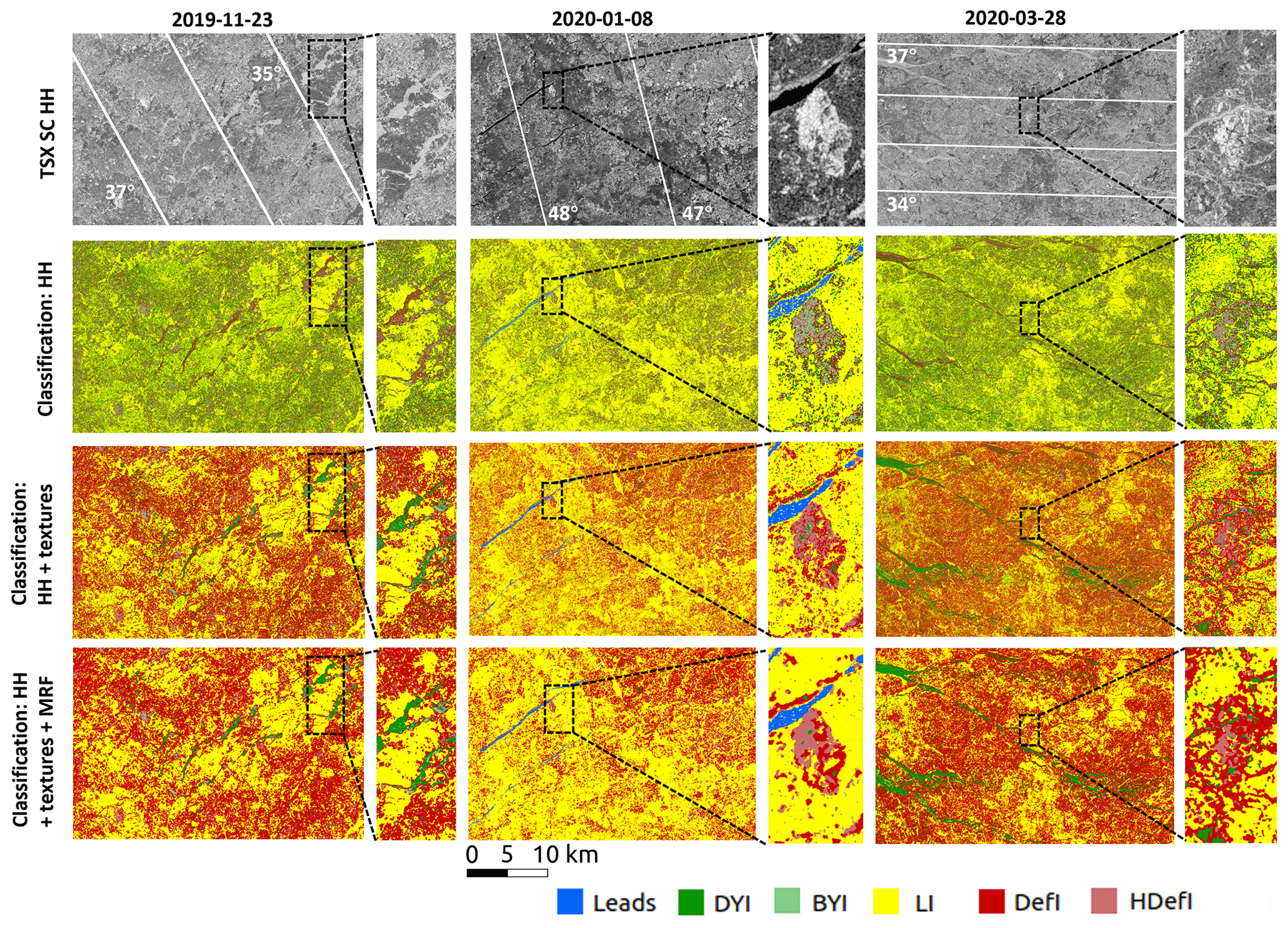
Figure 6 Example TSX SC scenes and classification maps using the GIA classifier trained with HH intensities only, HH intensities and optimal texture measures, and with MRF contextual smoothing applied for three scenes across the time series. IA contours are shown as white lines on HH intensities.

Overall classification accuracies for different testing scenes are shown as box plots in Fig. 7. The average overall accuracy for the classification of HH intensities and textures (78.31 %) is significantly higher (p value <0.01) than that of HH intensities only (64.79 %). The use of MRF contextual smoothing further increases (p value <0.01) the overall accuracy to 83.70 %. For the final classification with MRF contextual smoothing, the confusion matrix (not shown) indicates that remaining misclassifications mostly happen between the difficult class pairs, as expected. Leads and level ice are mostly correctly classified. The MRF contextual smoothing technique is theoretically (Doulgeris, 2015) and practically (not shown) superior to image smoothing processes that do not incorporate contextual information (e.g., a local majority filter) with respect to improving classification accuracy and minimizing the loss of spatial detail.

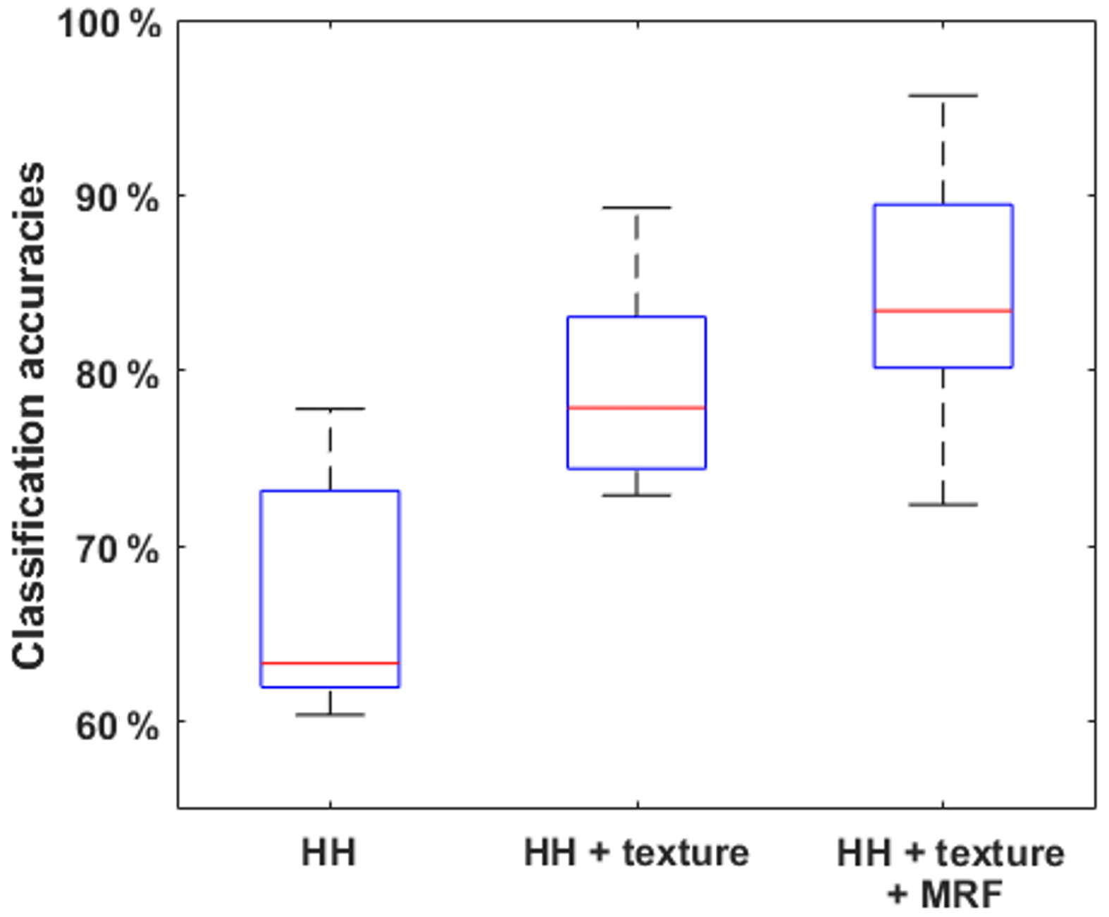
Figure 7 Overall accuracies for sea ice classification derived from testing scenes based on TSX SC HH intensities and on HH intensities and GLCM textures with and without MRF smoothing.

To demonstrate temporal classification consistency, classification maps for the middle of each month and the last scene of the time series (28 March 2020) are shown in Fig. 8. The general distribution of LI vs. DefI and HDefI is consistent through the time series for the classified scenes and the MOSAiC ice floe carrying the CO (zoomed-in patches). The classification maps clearly capture the breakup and the change in the size and shape of the MOSAiC ice floe. Major lead openings are seen on 17 and 28 March 2020, which are partially classified as BYI and DYI. Panoramic photos taken from RV Polarstern (Fig. 9b; Marcel et al., 2021) confirm the presence of ice openings occupied by young ice with the same position relative to the ship as indicated by Fig. 8, with RV Polarstern indicated by a black circle in the zoomed-in patches.

Figure 8 Classification maps of example TSX SC scenes; the zoomed-in patches focus on the MOSAiC ice floe, and black circles indicate the position of RV Polarstern.

A manual classification map of a small area around RV Polarstern is shown in Fig. 9a, which was produced by a co-author with extensive knowledge of sea ice conditions during MOSAiC. Our classification is consistent with the ground observations summarized in this map, indicating that the MOSAiC ice floe was composed of a mixture of FYI and second-year ice (SYI) and had a strongly deformed zone in the center (named “the Fortress”), which is the oval-shaped ice surface consistently classified as DefI and HDefI (Krumpen et al., 2020; Itkin et al., 2023). In most scenes in November 2019, part of the SYI surface of the MOSAiC ice floe surrounding the Fortress appears similar to or even darker than nearby LI (Fig. 8) and is, thus, classified as LI. This is attributed to the presence of refrozen melt ponds (Fig. 9a; Krumpen et al., 2021).

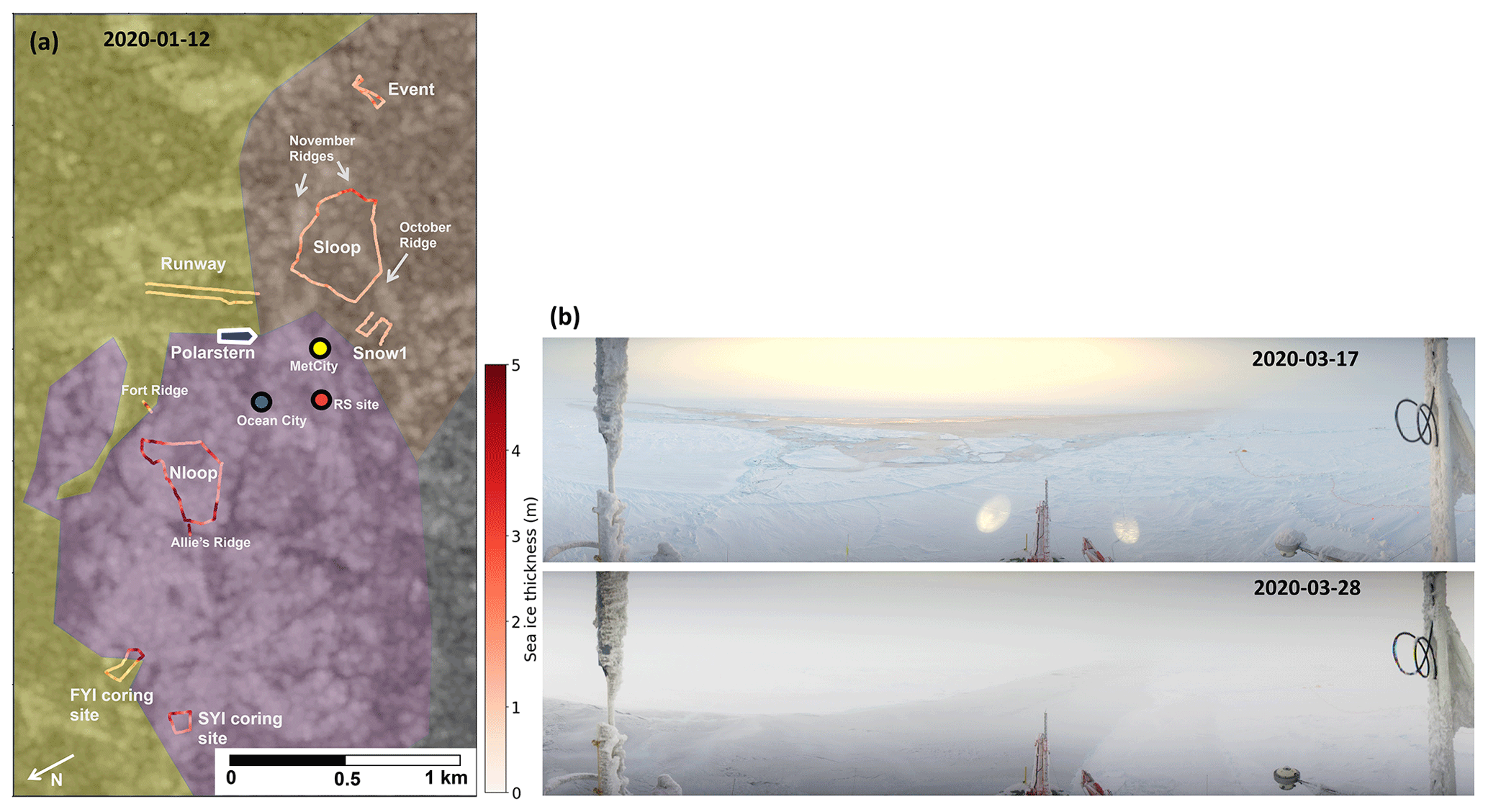
Figure 9 (a) Manual sea ice classification of the CO overlaid on a RS2 SCW scene (HH) on 12 January 2020. The color code used in the figure is as follows: yellow – FYI; purple – rough SYI; and red – ponded SYI. The RV Polarstern, weather stations, and transects with sea ice thickness measurements are also shown. Panel (b) shows two respective panoramic photographs taken from RV Polarstern on 17 and 28 March 2020.

3.2 Comparison to sea ice roughness estimates

The standard deviation of the sea ice thickness measured from the electromagnetic induction (EM) instrument (GEM-2; Hendricks et al., 2022) along several transects near the CO is used as a combined indicator of ice surface and bottom roughness and is plotted in blue on the classification maps in Fig. 10a. This dataset captures geometric roughness on the sea ice surface on the spatial scale of ice blocks or pressure ridges (i.e., approximately 1 to 30 m). Geographical coordinates from satellite images and ground data are converted to a local coordinate system that corrects for sea ice drift during data collection (Itkin et al., 2023). Additional minor manual translations are applied to account for geolocation errors. Nevertheless, some effects of ice floe rotation and deformation are present, and the data points are averaged in 4 pixel × 4 pixel windows (33 m×33 m) in TSX SC images to partially remedy these issues. Rougher ice (deeper blue) along the transects mostly corresponds correctly to areas classified as DefI or HDefI, and smoother ice (lighter blue) mostly corresponds correctly to LI (Fig. 10a).

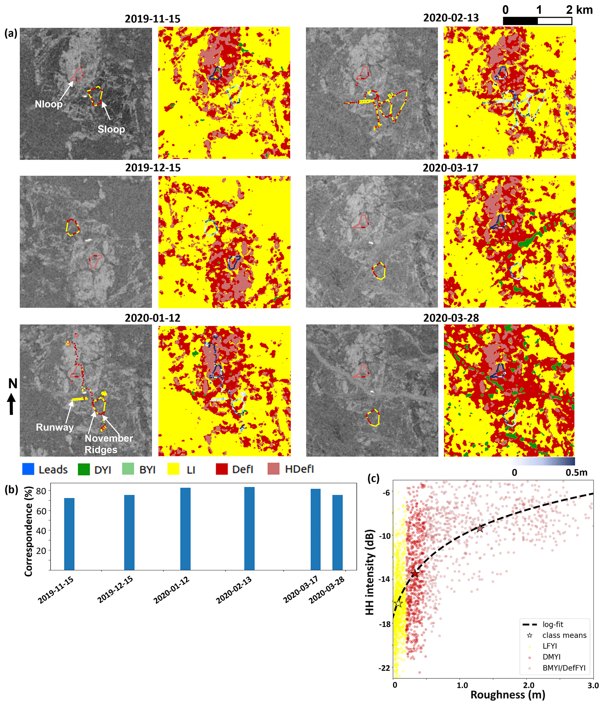
Figure 10 (a) Sea ice roughness in transects (in blue) overlaid on synthetic aperture radar (SAR) classification maps as well as the classification of sea ice roughness (in the same color scheme) overlaid on HH intensities in several transects within a 4 km × 4 km square around RV Polarstern for the same dates as those shown in Fig. 8; (b) the percentage correspondence between SAR and roughness classifications in repeated transects; and (c) a scatterplot of HH intensities vs. ice roughness in repeated transects, grouped by their corresponding class labels from the SAR classification.

Additionally, ice roughness transect points are classified into LI, DefI, and HDefI, as shown in Fig. 10a overlaid on HH intensities using the same color scheme as the SAR classification. This roughness classification is based on threshold values for level, rubble, and ridge ice, as described by Itkin et al. (2023). Briefly, in areas of mostly smooth FYI and SYI (outside the Fortress), ice roughness is classified into LI and DefI using a threshold of 0.2 m, showing good correspondence with LI and DefI in the SAR classification. In the Fortress, ice roughness is classified into DefI and HDefI using the same threshold, again showing a similar spatial distribution to DefI and HDefI in the SAR classification.

Two of the transects are repeated during the entire season: the southern and northern transect loops, or “Sloop” and “Nloop”, respectively (Fig. 10a). Sloop is located in the aforementioned ponded SYI area, and it crosses rough SYI and smooth refrozen melt ponds, which have similar HH intensities to LI, whereas Nloop is located in the Fortress and, thus, consists of predominantly heavily deformed SYI (Itkin et al., 2023). These observations are mostly correctly shown in both the SAR and roughness classifications. The “Runway” transect (Fig. 10a), established on LI, is also consistently classified as LI in both classifications.

The transect ice roughness estimate represents surface and bottom roughness, whereas the SAR classification represents only surface roughness. Consequently, there is an apparent mismatch between the two classifications that can be seen, for example, in Sloop on the “November ridges”, as indicated by arrows in Fig. 10a, most notably on 12 January 2020. In the southern part of Sloop (arrow to the right), where ice is smooth but thick, low HH intensities lead to the SAR classification result of LI, but the roughness classification result is DefI, presumably due to the dominance of ice-bottom roughness. On the contrary, in the western part (arrow to the left), high HH intensities and, hence, a rough ice surface lead to a SAR classification of DefI, whereas the roughness classification result is mostly LI, likely due to low thickness standard deviations calculated from thin ice (Fig. 9a).

The percentage of correct correspondence between both classifications in repeated transects is shown in Fig. 10b. Corresponding to a roughness classification data point, the SAR classification is counted as “correct” if the ice class of at least one TSX pixel in its surrounding 4 pixel × 4 pixel window is the same class. Good correspondence is found between the two classifications, with the percentages of correctly classified SAR pixels being consistently near or more than 80 %.

Finally, we demonstrate the relationship between HH intensities and ice roughness for the repeated transects, grouped by class labels from the SAR classification (Fig. 10c). An apparent logarithmic fit can be seen, where the points representing mean roughness and intensities for LI, DefI, and HDefI (shown using stars) are very close to the fitted curve. This indicates that TSX SC HH intensities in these particular transects are largely controlled by geometric ice roughness because other sea ice surface properties, such as micro-roughness (centimeter to decimeter), salinity, and snow, are quite similar. This relationship as well as the good correspondence between the SAR and roughness classifications shown by Fig. 10c and the above qualitative comparisons illustrate that, under similar environmental conditions, TSX SC HH intensities of FYI and MYI can be attributed to different degrees of deformation, which justifies our chosen classification scheme. Previous studies have also found a similar logarithmic relationship between geometric surface roughness and SAR backscatter intensities for winter sea ice for co- and cross-polarization channels of C- and L-band SAR sensors (Cafarella et al., 2019; Segal et al., 2020), whereas microscale roughness has a more significant impact on C-band backscatter than on the L-band (e.g., Dierking and Dall, 2007; Gegiuc et al., 2018). It is expected that the TSX signal, with a shorter wavelength than C-band sensors, should also react to small-scale roughness, but quantifying the contrast between the influence of different spatial scales of surface roughness on SAR backscatter is not achievable with the observations used here, nor is it within the scope of this study. The contribution from both surface and bottom roughness to our ice roughness estimate as well as the additional influence from small-scale surface roughness presumably leads to the relatively wide spread of the scatterplot.

3.3 The temporal development of ice class fractions

Areal fractions of different classes for all scenes in the time series are shown in Fig. 11. Leads, DYI, and BYI are combined into a “lead ice” category, representing areas of ice opening. DefI and HDefI are combined into a “deformed ice” category. Relative proportions of level vs. deformed ice are reasonably consistent through the time series (Fig. 11). Several peaks in the lead ice fraction are visible, most notably in middle to late November 2019 and late January to early February 2020. In March 2020, lead ice fractions remain high and ice openings can be consistently observed in the scenes. A major ice-opening event occurred on 28 March 2020 (Fig. 8) during which time the lead ice fraction reached 7.16 %. This event persisted through early April.

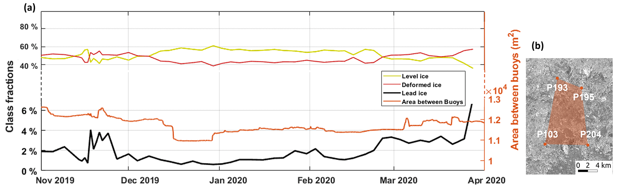
Figure 11 (a) Fractions of level ice, deformed ice, and lead ice (left y axis) as well as the areas between four buoys surrounding the CO (right y axis) over the time series; (b) the names and positions of the four buoys are shown for 1 November 2019.

A detailed examination of ice-opening events is conducted by comparing the class fractions to indicators of ice openings derived in this work and in other MOSAiC studies:

1. Areal change between buoys. The area between four selected buoys (P103, P193, P195, and P204; Fig. 11b) surrounding the CO (Bliss et al., 2021) is calculated every 3 h, partially representing events of divergence and convergence (Fig. 11a, orange). Similar peaks in this areal change to those of the lead ice fractions can be seen in middle to late November (Fig. 11). Areal changes are also frequent through March, indicating frequent short-lived ice openings between the buoys. The sharp decrease in the area on 15 December 2019 is caused by a large-scale shearing event that lasted through to 23 December 2019 but is not prominently registered by changes in the lead ice fraction in the scenes due to significantly larger spatial scales.

2. Other MOSAiC studies. Several peaks in the lead ice fractions in Fig. 11a have good correspondence with those generated from optical satellite observations shown in Krumpen et al. (2021). Lead fractions within a 50 km radius of the CO show prominent peaks in early to middle December, early February, and early and late March, matching those in Fig. 11. In the same study, no lead fraction is produced for middle to late November and middle to late March, but prominent divergence and convergence events can be seen in middle to late November and late March, as obtained from S1 sea ice drift data (Krumpen et al., 2021). Similar to our study, a recent sea ice classification study on TSX dual-polarization Stripmap (SM) images (54 km × 16 km at a 3.5 m resolution) also identifies a prominent rise in young-ice fractions in the 3 km × 3 km area around RV Polarstern in late November 2019 and late March 2020 (Kortum et al., 2022). Abrupt and prominent changes in wind speed and direction were recorded from RV Polarstern during these periods (Itkin et al., 2023), which likely contributed to the observed increase in lead-opening events.

These comparisons demonstrate that our classified time series is valuable as an indicator of ice openings; thus, it is a good reference for studying the associated physical processes over a larger spatial scale than the previously derived MOSAiC sea ice classification product (Kortum et al., 2022).

3.4 Limitations and future steps

The current classifier has a limited capability with respect to detecting linear young-ice areas that are narrower than the texture window size. This is an inevitable outcome of texture-based classification that we try to mitigate by minimizing texture windows. Comparatively, the leads class is mostly fully represented in the classification, as it is classified with HH intensities only. The texture parameter selection workflow established in this study produces satisfactory classification results (Sect. 3.1, 3.3) and is generally applicable to future studies. However, the texture parameters yielded are specific to our dataset on the constrained IA range of the training scenes.

The inherent scalloping and inter-scan banding issues in ScanSAR products can be observed in HH intensities and textures with varying visibility across scenes and are more prominent in HH textures than in HH intensities. These image artifacts affect the classification results, most notably leading to misclassification between the difficult class pairs. This issue is partially remedied by MRF contextual smoothing. For future studies using TSX SC scenes with obvious sensor artifacts, additional correction steps should be taken using previously proposed procedures (e.g., Iqbal et al., 2012; Yang et al., 2020).

No continuous in situ observation is available to provide detailed information on thin ice evolution through the time series. Ice roughness derived from in situ ice thickness measurements is calculated on a different spatial scale from that of the classification maps, represents both surface and bottom ice roughness, and suffers from potential co-location errors due to sea ice rotation and deformation. Therefore, the utilization of ice surface roughness calculated from airborne and ground-based laser scanners is desirable in future studies as a stronger validation of ice classification. This study has focused on the freezing season during the MOSAiC expedition. Future steps will extend the study period into summer to examine the seasonality of TSX SC textures of sea ice and its effects on texture-based sea ice classification.

For future studies on texture-based sea ice classification, more detailed quantification of the correspondence between GLCM textures and ice surface properties should be conducted, following previous studies (e.g., Baraldi and Parmiggiani, 1995; Soh and Tsatsoulis, 1999). Moreover, previous studies of texture-based sea ice classification have achieved ice-type separation using various physical window sizes. Therefore, investigation into the better inclusion of multiscale textural information (e.g., by varying window size and co-occurrence distance) is desirable (e.g., Soh and Tsatsoulis, 1999; Leigh et al., 2014). Although GLCM textures are among the most powerful tools for texture-based classification (Hall-Beyer, 2017; Zakhvatkina et al., 2019), it is still valuable to examine IA dependencies and the utilization of other types of image textures previously used for sea ice classification, such as first-order textures; image moments; and MRF-based, wavelet-transformed-based, variogram-based, and gray-level-dependence-matrix-based textures (Conners and Harlow, 1980; Unser, 1995; Clausi, 2001; Clausi and Yu, 2004; Sanden and Hoekman, 2005; Bogdanov et al., 2007; Komarov and Buehner, 2017; Gegiuc et al., 2018; Scharien and Nasonova, 2020). Finally, the integration of ice-type-specific IA dependencies into other classifiers, such as convolutional-neural-network-based classifiers (e.g., Boulze et al., 2020), is desirable to potentially improve classification performance.

4 Conclusions

This study demonstrates per-class IA slopes of HH intensities and GLCM textures calculated from TSX SC data, and it uses a sea ice classifier incorporating these IA dependencies to produce a classified time series for the winter MOSAiC period. Linear IA dependencies of HH intensities in decibels in our study area and period are generally lower than C-band data, but between-class IA slope differences still necessitate per-class IA correction. In the constrained IA range, GLCM textures calculated from decibel intensities also exhibit linear IA dependencies. The leads class has a wide scatter in HH intensities and textures vs. IAs, resulting in weak linear dependency, and is, thus, retrieved from a separate classification on HH intensities only. A texture parameter selection process based on statistical separability between class distributions determines the optimal texture combination to be DIS, ENG, ENP, HOM, MAX, SMA, and VAR (see Table 2 for definitions) at a window size of nine pixels with a co-occurrence distance of two pixels. We use a classification scheme that separates young ice into different SAR intensities and separates FYI and MYI into different deformation states. Qualitative assessments via visual inspection of classification maps and quantitative assessment using classification accuracies show that the inclusion of GLCM textures is essential for classifying single-polarization TSX SC data. The application of MRF contextual smoothing refines the result while preserving maximum spatial details, leading to significantly increased classification accuracies. Good correspondence is found between the classification result and geometric ice roughness calculated from in situ ice thickness measurements, with the latter showing a logarithmic relationship with HH backscatter intensities. The classified time series shows reasonably consistent fractions of LI vs. DefI and HDefI. Lead ice fractions derived from the classification result correspond well to other indicators of ice openings derived in this work and in previous studies. This suggests that the classified time series can serve as a reliable reference of the sea ice conditions and associated physical processes during the expedition within the spatial scale of the TSX SC scenes. This study provides valuable information on the utilization of per-class IA dependencies of TSX SC intensities and GLCM textures in classifying sea ice as well as a classification product incorporating a broad area surrounding the MOSAiC ice camp that can potentially facilitate future MOSAiC sea ice studies and modeling efforts.