The response of sea ice and high-salinity shelf water in the Ross Ice Shelf Polynya to cyclonic atmosphere circulations

Coastal polynyas in the Ross Sea are important source regions of high-salinity shelf water (HSSW) – the precursor of Antarctic Bottom Water that supplies the lower limb of the thermohaline circulation. Here, the response of sea ice production and HSSW formation to synoptic-scale and mesoscale cyclones was investigated for the Ross Ice Shelf Polynya (RISP) using a coupled ocean–sea ice–ice shelf model targeted on the Ross Sea. When synoptic-scale cyclones prevailed over RISP, sea ice production (SIP) increased rapidly by 20 %–30 % over the entire RISP. During the passage of mesoscale cyclones, SIP increased by about 2 times over the western RISP but decreased over the eastern RISP, resulting respectively from enhancement in the offshore and onshore winds. HSSW formation mainly occurred in the western RISP and was enhanced responding to the SIP increase under both types of cyclones. Promoted HSSW formation could persist for 12–60 h after the decay of the cyclones. The HSSW exports across the Drygalski Trough and the Glomar Challenger Trough were positively correlated with the meridional wind. Such correlations are mainly controlled by variations in geostrophic ocean currents that result from sea surface elevation change and density differences.

1 Introduction

Antarctic coastal polynyas are characterized by the areas of persistent open water surrounded by sea ice along the coastlines, which tend to appear recurrently at fixed geographical locations and periods of the year. These coastal polynyas are mechanically driven by offshore katabatic and synoptic winds (Bromwich et al., 1998; Massom et al., 1998; Morales Maqueda et al., 2004), which are regarded as the dominant near-surface wind fields over the Antarctic continent. Katabatic wind is traditionally defined as a downslope cold flow driven by gravity and pressure gradient force over a sloping surface near the Antarctic coast, and its direction is largely controlled by local topography (Lutgens and Tarbuck, 2001). New sea ice production within coastal polynyas and the associated brine rejection process leads to the formation of high-salinity shelf water (HSSW), which is the precursor of Antarctic Bottom Water (AABW), a key component of the lower cell of the meridional overturning circulation (Comiso and Gordon, 1998; Ohshima et al., 2013; Whitworth et al., 2013). Furthermore, Antarctic coastal polynyas are identified as biological “hot spots” due to the enhanced primary productivity during the austral spring and summer (Arrigo and van Dijken, 2003). The polynya regions are also characterized by massive atmospheric CO₂ sinking (Hoppema and Anderson, 2007; Arrigo et al., 2008; Tortell et al., 2012), resulting from deep convection and large amounts of phytoplankton accumulation compared with adjacent waters (Tremblay and Smith, 2007). Consequently, coastal polynya processes play an important role in the global climate system.

Previous studies indicate that the sea ice production (SIP) rate and HSSW formation within the coastal polynyas are significantly increased with the strength of katabatic winds (Mathiot et al., 2010; Barthélemy et al., 2012; Zhang et al., 2015; Dale et al., 2017; Cheng et al., 2019). Most of these studies focused on the role of winds in the Antarctic coastal polynyas on seasonal or longer timescales. However, atmospheric conditions along the Antarctic coast are characterized by high-frequency wind events associated with the passages of synoptic-scale or mesoscale cyclones (Turner et al., 2009; Chenoli et al., 2015; Weber et al., 2016; Wang et al., 2021). The coastal margin of Antarctica is regarded as the most active cyclogenetic region on earth due to the existence of a strong baroclinic zone around the Antarctic continent (Parish and Cassano, 2003). The coastal Ross Sea, which has been identified as an important source region of AABW due to the presence of the Terra Nova Bay and Ross Ice Shelf polynyas (Jacobs et al., 1970; Gordon and Comiso, 1988; Whitworth and Orsi, 2006), is frequently affected by the passages of cyclones (Bromwich et al., 1993; Simmonds et al., 2003; Knuth and Cassano, 2011; Uotila et al., 2011; Yu and Zhong, 2019). Recent studies have begun to focus on the influence of synoptic-scale wind forcing on sea ice properties in the Ross Sea polynyas based on the observations (Dale et al., 2017; Cheng et al., 2019; Ding et al., 2020; Thompson et al., 2020; Wenta and Cassano, 2020). The sea ice properties and the polynya extent have a strong correlation with wind speed in the Ross Sea polynyas (Dale et al., 2017; Cheng et al., 2019; Ding et al., 2020). Thompson et al. (2020) demonstrated that the estimated frazil ice production could increase up to 110 cm d⁻¹ during the strongest wind events using in situ observations, available from the Polynyas and Ice Production and seasonal Evolution in the Ross Sea (PIPERS) program, which conducted an autumn ship campaign in 2017 and two spring airborne campaigns in 2016 and 2017 (Ackley et al., 2020). Wenta and Cassano (2020) found that during an extreme wind event associated with the passage of two cyclones, the extent of the Terra Nova Bay (TNB) polynya increased dramatically by over 20-fold. These studies provide important insights into the response of polynyas to changes in atmospheric forcing. However, the influence of cyclones on the oceanic processes, including the convection and the formation of HSSW that directly affect the AABW and thermohaline circulation, has not been revealed. Moreover, different types and paths of cyclones may induce different coastal wind patterns over the polynyas and result in distinct responses by sea ice production and the HSSW formation. The extent of these processes remains uncertain but would be important for understanding the short-scale variability of HSSW and even the AABW formation.

As very few in situ measurements have been conducted at the Antarctic coastal polynyas during the freezing season, numerical models have become indispensable methods to investigate the response of sea ice and oceanic processes to harsh weather conditions, such as cyclones. In this study, a 5 km resolution regional ocean–sea ice–ice shelf model for the Ross Sea was employed to investigate the role of mesoscale and synoptic-scale cyclones in sea ice production and the HSSW formation in the Ross Ice Shelf Polynya (RISP), which is the largest coastal polynya with the highest SIP over the Southern Ocean (Tamura et al., 2008; Kern et al., 2009). This paper is organized as follows. In Sect. 2, descriptions of the numerical model, observational data, and model validation and analysis methods are provided. In Sect. 3, the impacts of different types of cyclones on the variations of sea ice production and water mass formation are presented and interpreted. Discussions on the HSSW exports in the troughs that are major conduits for HSSW outflow and their relationship with the meridional winds are also given in Sect. 3. Section 4 provides the conclusions.

2 Data and methods

2.1 Model data description

This study utilizes the Ross Sea circulation model as described in Dinniman et al. (2018), which is implemented with the Regional Ocean Modeling System (ROMS). ROMS combines a primitive-equation, finite-volume ocean model with a dynamic sea ice model (Budgell, 2005) based on an elastic–viscous–plastic (EVP) rheology solver (Hunke and Dukowicz, 1997; Hunke, 2001). The sea ice model applies the two-layer ice thermodynamics following Mellor and Kantha (1989) and Häkkinen and Mellor (1992), which has been verified to be able to simulate sea ice variables well over coastal regions around the Antarctic including the Ross Sea (Stern et al., 2013; Dinniman et al., 2011, 2015). The ice shelves used in this model are static, which means that the motion or mass change of the ice sheet, including iceberg calving, is ignored. The thermodynamic and mechanical effects of the Ross Ice Shelf (RIS) cavity on the adjacent water beneath are parameterized (Holland and Jenkins, 1999; Dinniman et al., 2011). The momentum, heat, and freshwater (imposed as a salt flux) fluxes in the open ocean are calculated from the COARE version 3.0 bulk flux formulae (Fairall et al., 2003). There is no relaxation for surface temperature or salinity towards prescribed values, such as an observational climatology.

The southern extent of the Ross Sea model domain includes most of the cavity under the RIS, and the northernmost part consists of the continental shelf break and extends to 67.5^∘ S (Fig. 1). The model has a horizontal resolution of 5 km and 24 vertical layers with variable thicknesses (higher resolution towards the top and bottom surfaces) based on a terrain-following vertical coordinate system (Haidvogel et al., 2008; Shchepetkin and McWilliams, 2009). The topographic datasets used in this model are from the International Bathymetric Chart of the Southern Ocean (IBCSO) and Bedmap2 (Arndt et al., 2013; Fretwell et al., 2013) which include the elevation of the bedrock and the base of any floating ice shelves (mainly for the RIS). The lateral open boundary conditions for temperature and salinity are derived from the climatological data based on the World Ocean Atlas 2001 (WOA01) and for barotropic velocities from the Ocean Circulation and Climate Advanced Modelling project (OCCAM; Saunders et al., 1999). Monthly observed data from passive microwave satellite observations (SSM/I) over 1999–2014 are used as the lateral open boundaries for sea ice concentration. Ocean tidal currents and the inverse barometer effect are not included. The atmospheric forcing fields, including 6-hourly winds and air temperature and monthly sea level pressure and humidity, were obtained from the ERA-Interim reanalysis product (Dee et al., 2011) produced by the European Centre for Medium-Range Weather Forecasts (ECMWF) (Dinniman et al., 2018). The high temporal resolution for winds and air temperature is related to their importance for simulating sea ice and currents in the Southern Ocean (Wu et al., 2020). Coastal precipitation from reanalysis products for Antarctica is significantly affected by atmospheric model resolution (van Lipzig et al., 2004). Therefore, monthly climatological precipitation used in this model is derived from the Antarctic Mesoscale Prediction System (AMPS), a high-resolution atmospheric model over the Antarctic (Powers et al., 2003; Bromwich et al., 2005), instead of the ERA-Interim product. Furthermore, due to the overestimation of mean clouds over the Southern Ocean from ERA-Interim, monthly cloud fraction climatology data come from the International Satellite Cloud Climatology Project stage D2 (ISCCP D2; Rossow et al., 1996) and are used to calculate net longwave and shortwave radiation following Berliand (1952). These atmospheric variables are used in the bulk formulae to generate the surface fluxes in the Ross Sea model (Fairall et al., 2003). The ERA-Interim has a spectral T255 horizontal resolution which corresponds to approximately 79 km spacing on a reduced Gaussian grid. The ERA-Interim reanalysis products can well resolve the mesoscale and synoptic-scale cyclones (Uotila et al., 2013; Chenoli et al., 2015; Yu and Zhong, 2019). The Ross Sea model simulation spans from 15 September 1999 to 15 September 2014 after a 6-year spin-up simulation, and the model results are output as 5 d average values. In this study, for the selected periods of synoptic-scale or mesoscale atmospheric events, model simulations over June to September of 2005 and 2014 are output as 6-hourly results, which is essential to revealing the detailed processes over the short duration of the cyclone events.

2.2 Observational data for model validation

In this work, the simulated sea ice concentration in the RISP was validated by the daily bootstrap sea ice concentrations from Nimbus-7 SMMR and DMSP SSM/I-SSMIS archived at the National Snow and Ice Data Center (NSIDC) (Markus and Cavalieri, 2000; Comiso, 2017), which have a horizontal resolution of 25 km (https://nsidc.org/data/nsidc-0079/versions/3, last access: 15 January 2023). The Advanced Microwave Scanning Radiometer for the Earth Observing System (AMSR-E)-product-derived SIP was employed to evaluate the modeled SIP. The AMSR-E SIP is estimated based on the heat flux calculation using a thin-ice-thickness estimation algorithm and surface atmospheric data (http://www.lowtem.hokudai.ac.jp/wwwod/polar-seaflux/, last access: 8 February 2023), assuming that the contribution of oceanic heat flux to the sea ice freezing–melting process is negligible (Nihashi and Ohshima, 2015; Nihashi et al., 2017). The AMSR-E SIP dataset was calculated over 2003–2010, and the annual cumulative SIP is defined as the integrated ice production from March to October, i.e., the freezing season (Nihashi and Ohshima, 2015). Wind speeds at 10 m from the ERA-Interim reanalysis were compared with measured 10 m wind data at the McMurdo Station near the Ross Island (Fig. 1b) over austral winter. The observed wind speed data are available on the Reference Antarctic Data for Environmental Research (READER) project website (https://legacy.bas.ac.uk/met/READER/, last access: 12 November 2022). We selected two winters to study the influence of cyclone events, which are featured by high correlations between wind speed from ERA-Interim and observations (correlation coefficients R>0.5 and p values P<0.0001) and have representative mesoscale or synoptic-scale cyclone events. The selected years were 2005 (R=0.56) and 2014 (R=0.61).

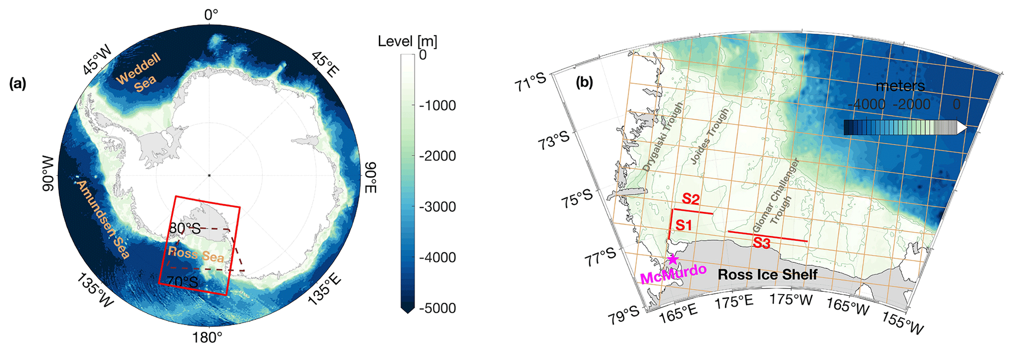
Figure 1 Geographic map of (a) the Southern Ocean south of 60^∘ S, and (b) the Ross Sea. Areas in white show continental surfaces, and areas in light grey indicate the ice shelves. The color scale indicates the bathymetry. In panel (a), the Ross Sea model domain is shown by the solid red box, and the dashed brown box represents the area shown in panel (b). In panel (b), the orthogonal yellow lines indicate the model grids magnified by a factor of 20, the magenta star indicates the position of McMurdo Station, and the red lines indicate the S1, S2, and S3 sections crossing the troughs that are the major passages for HSSW outflows towards the slope.

2.3 Model validation

The performance of the Ross Sea model in reproducing sea ice properties in the RISP was evaluated by comparing the annual cumulative SIP from the model simulation with the estimates from satellite data. Following Nihashi and Ohshima (2015), the calculation of annual cumulative SIP covers the period of March to October, i.e., the ice-freezing seasons for the Southern Ocean. The annual cumulative SIP averaged over 2003–2010 in the RISP presents similar spatial patterns between the simulation and observations (Fig. 2a–b). Compared with the observations, the model slightly overestimates the SIP, which is a common problem with the Southern Ocean ocean–sea ice models used for studying Antarctic coastal polynyas (Zhang et al., 2015; Kusahara et al., 2017; Wang et al., 2021). The integrated SIP volumes over the RISP are 6.79×10² and 6.10×10² km³ yr⁻¹ for modeled and observed datasets respectively. Such a SIP overestimation is possibly associated with the relatively coarse resolution of the atmospheric forcing fields compared to the actual wind conditions. The atmospheric model with too low a resolution possibly extends orographic slopes seaward, beyond the actual coastline, and thus induces offshore winds that are too strong, which in turn enhance SIP in the coastal polynyas (Stössel et al., 2011). In addition, the AMSR-E SIP product does not discriminate the active-frazil area for Antarctic coastal polynyas, which could result in an underestimation of sea ice production for frazil-dominant polynyas (Nakata et al., 2021). Statistical analysis of comparisons for daily SIC anomalies in winters (June–September) of 2005 and 2014 from climatological values was conducted, and the results are shown in Fig. 2c and d. Correlation coefficients between the modeled and observed sea ice concentration in RISP in 2005 and 2014 are 0.45 (P<0.001) and 0.73 (P<0.0001), respectively (Figs. 2c–d), suggesting that the model captures the daily variability of ice concentration well. The absolute deviations of modeled ice concentration are −0.31 and −0.29 for 2005 and 2014 respectively.

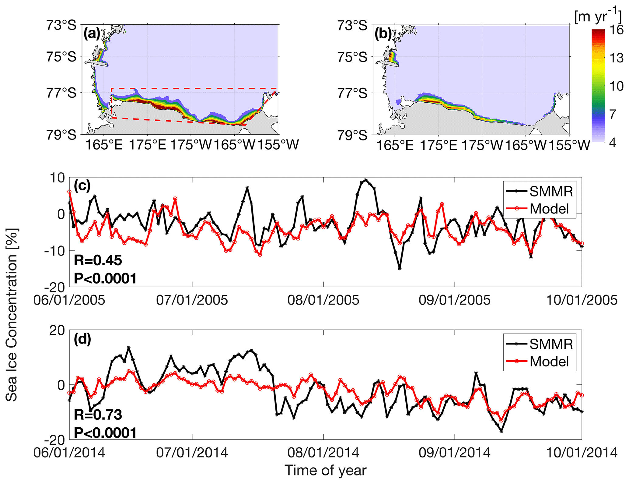
Figure 2 (a–b) Annual cumulative sea ice production rates over the Ross Sea from (a) the Ross Sea model and (b) the AMSR-E product averaged over 2003–2010. The polygon in panel (a) enclosing the Ross Ice Shelf Polynya was used to analyze the HSSW characteristics. (c–d) Time series of observed (black lines) and modeled (red lines) daily polynya-averaged sea ice concentration anomalies in June–September of 2005 and 2014.

2.4 Analysis methods

The extent of RISP was defined as the area where the multi-year-average annual cumulative SIP is greater than zero near the RIS region based on the Ross Sea model results. The HSSW is defined as the water mass with neutral density (γⁿ) above 28.27 kg m⁻³, practical salinity (S) >34.62 and potential temperature (θ) $<-\mathrm{1.85}$ ^∘C (Orsi and Wiederwohl, 2009; Castagno et al., 2019). Temperature–salinity (T–S) analysis and the calculations of HSSW volume and spatial-averaged HSSW salinity were conducted over the defined RISP polygon region presented in Fig. 2a, to elucidate the impacts of cyclones on the HSSW formation. The HSSW export rates were calculated across three transects (Fig. 1b) located over three troughs, the Drygalski Trough (S1), the Joides Trough (S2), and the Glomar Challenger Trough (S3), that are the major HSSW outflow passages.

Cyclones were tracked by the University of Melbourne Automatic Cyclone Tracking Scheme (Murray and Simmonds, 1991), based on the ERA-Interim reanalysis product from 1999 to 2014. The optimal parameters used in this scheme, including the horizontal air pressure field smoothing parameter, the radius used for the calculation of Laplacian pressure, and the maximum topographic height for detecting the cyclones, adopted the values by Uotila et al. (2009). The identified cyclone properties included their locations, lifetimes, and mean radii. Cyclones were selected according to the criteria that they should have lifetimes longer than 12 h and the distance between their first and last detected locations should be greater than 1000 km. Such criteria are likely to exclude detected but unrealistic cyclones (Uotila et al., 2011). We divided the area south of 42^∘ S into 720 sectors, each one spanning 4^∘ in latitude and 6^∘ in longitude, and calculated cyclone track densities, defined as the number of cyclone tracks per each sector (Uotila et al., 2013) over 1999 to 2014 (Fig. 3). The cyclones were categorized into two types depending on their horizontal scale: synoptic-scale cyclones with length scales 1000 km or longer and mesoscale cyclones with length scales shorter than 1000 km (Heinemann, 1990; Bromwich, 1991; Carrasco et al., 2003; Uotila et al., 2011). The synoptic-scale depressions form mainly on stronger horizontal temperature gradients in the troposphere and grow through baroclinic instability. The mesocyclones are usually the cold air vortices forming to the south of the main polar front and develop in outbreaks of polar air. In this study, we selected two representative synoptic-scale cyclone events that had different paths over the study region and one mesoscale cyclone event. These three events occurred in June 2005 (labeled as MESO), July 2005 (labeled as SYNO1), and September 2014 (labeled as SYNO2).

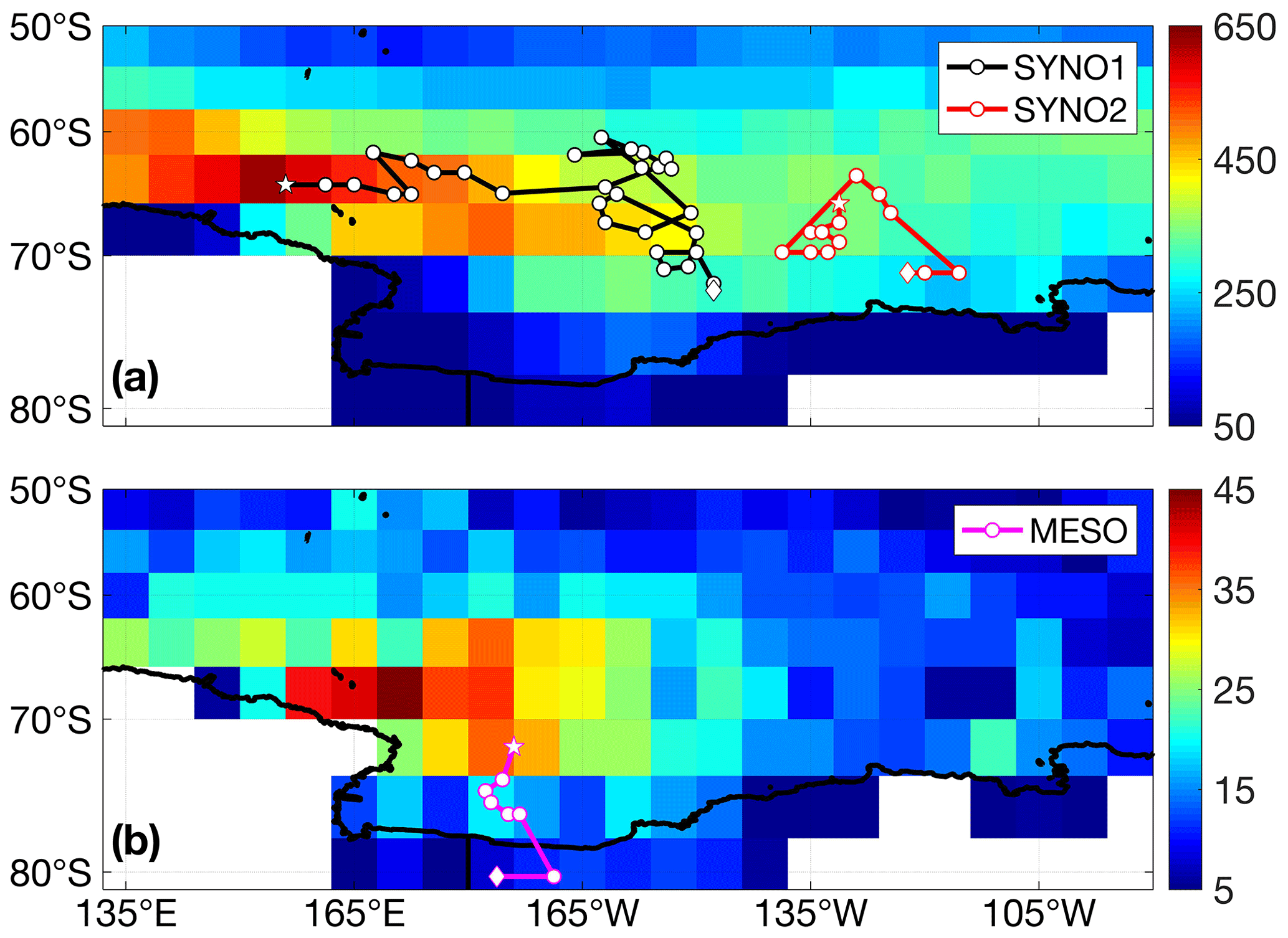
Figure 3 Accumulated track densities (the number of tracks per section) of (a) synoptic-scale cyclones and (b) mesoscale cyclones in the Ross Sea and surrounding regions over 1999–2014. The black, red and magenta lines indicate complete cyclone trajectories of selected cases (SYNO1, SYNO2, and MESO), and the circles represent the 6-hourly cyclone center locations, the pentacles indicate the starting positions and the diamonds present the ending positions.

A three-dimensional momentum analysis of ocean flow was conducted to elucidate the potential mechanisms for the HSSW export variability under the impact of a typical cyclone. Each momentum term was analyzed to diagnose the dominant term related to the export variability. The three-dimensional along-ice-shelf and across-ice-shelf (defined by local acceleration terms) momentum equations are

$$\begin{array}{}\text{(1)}& \begin{array}{rl}{\displaystyle \frac{\partial u}{\partial t}}& =-\left(u{\displaystyle \frac{\partial u}{\partial x}}+v{\displaystyle \frac{\partial u}{\partial y}}+w{\displaystyle \frac{\partial u}{\partial z}}\right)+fv-{\displaystyle \frac{\mathrm{1}}{{\mathit{\rho }}_{\mathrm{0}}}}{\displaystyle \frac{\partial p}{\partial x}}\\ & +K_{\mathrm{V}}{\displaystyle \frac{{\partial }^{\mathrm{2}}u}{\partial z^{\mathrm{2}}}}+K_{\mathrm{H}}\left({\displaystyle \frac{{\partial }^{\mathrm{2}}u}{\partial x^{\mathrm{2}}}}+{\displaystyle \frac{{\partial }^{\mathrm{2}}u}{\partial y^{\mathrm{2}}}}\right)\end{array}\end{array}$$

and

$$\begin{array}{}\text{(2)}& \begin{array}{rl}{\displaystyle \frac{\partial v}{\partial t}}& =-\left(u{\displaystyle \frac{\partial v}{\partial x}}+v{\displaystyle \frac{\partial v}{\partial y}}+w{\displaystyle \frac{\partial v}{\partial z}}\right)-fu-{\displaystyle \frac{\mathrm{1}}{{\mathit{\rho }}_{\mathrm{0}}}}{\displaystyle \frac{\partial p}{\partial y}}\\ & +K_{\mathrm{V}}{\displaystyle \frac{{\partial }^{\mathrm{2}}v}{\partial z^{\mathrm{2}}}}+K_{\mathrm{H}}\left({\displaystyle \frac{{\partial }^{\mathrm{2}}v}{\partial x^{\mathrm{2}}}}+{\displaystyle \frac{{\partial }^{\mathrm{2}}v}{\partial y^{\mathrm{2}}}}\right),\end{array}\end{array}$$

respectively, where u and v are the along-ice-shelf and across-ice-shelf components of velocity, f is the Coriolis parameter, ρ₀ is the reference density of 1025 kg m⁻³, p is pressure, x is the along-shelf coordinate, y is the cross-shelf coordinate, and K_V and K_H are the vertical and horizontal eddy viscosity coefficients respectively. Vertical momentum and tracer mixing were calculated using the K profile parameterization (KPP; Large et al., 1994). Each term of the momentum equations was calculated for each model time step and output as 6-hourly averages. In addition, the geostrophic currents may be either barotropic or baroclinic. Then to elaborate on which component dominates the variation of HSSW export, the barotropic flow related to the changes in sea surface and the baroclinic flow resulting from the density differences were calculated.

3 Results and discussions

3.1 Cyclone track densities

The track density of synoptic-scale cyclones can be up to 10–14 times higher than that of mesoscale cyclones in the Ross Sea and the surrounding regions (Fig. 3). Such discrepancy between synoptic-scale and mesoscale cyclones could be related to the relatively coarse spatial resolution of the ERA-Interim product, which may not capture all smaller systems like mesoscale cyclones (Condron et al., 2006; Uotila et al., 2009, 2011). However, the spatial distributions of cyclones revealed in this study are consistent with the features in Uotila et al. (2011), which are derived from the AMPS high-resolution dataset. The high track density of synoptic-scale cyclones extends to the continental slope regions of the western Ross Sea (at around 65^∘ S, Fig. 3a). For mesoscale cyclones, on the Ross Sea continental shelf a large number of track densities appear in front of the RIS central region (near the ∼180^∘ meridian, Fig. 3b), which may be related to the cold air outbreaks from the continental interior (Seefeldt and Cassano, 2008; Turner et al., 2009). For synoptic-scale cyclones, two events were selected for our study, which occurred in July 2005 (SYNO1) and September 2014 (SYNO2) respectively. SYNO1 was formed as a combination of two synoptic-scale cyclones with relatively small spatial scales by examining the spatial distribution of sea level pressure. The initial low-pressure center originated in the area about 65^∘ S northwest of the Ross Sea. Afterward, this system gradually developed to the north of the central Ross Sea and then moved southeastwards before finally reaching the eastern coastal region. The complete trajectory of SYNO1 is represented in Fig. 3a. The path of the cyclone related to this event was located in the area with high track densities shown in Fig. 3a. The onset and development of SYNO2 in the September 2014 event were primarily situated along the northeastern part of the Ross Sea (about 130^∘ W), accompanied by a slight east–west movement (Fig. 3a). Although the latter event has quite a different trajectory than the earlier one, it was also located in the high-track-density area over the eastern region (Fig. 3a). For the mesoscale system, we chose one representative event occurring in June 2005 (MESO). This cyclone moved southeastward from the northern continental shelf region and lingered in the central Ross Sea, where the track density is higher compared to nearby areas (Fig. 3b).

3.2 Synoptic-scale cyclones

3.2.1 The SYNO1 case

As mentioned in Sects. 2.4 and 3.1, two representative synoptic-scale cyclones were selected over the Ross Sea region in the freezing season of 2005 and 2014 respectively. The SYNO1 occurred from 13 July to 17 July of 2005, when the cyclone was situated in a mature stage, i.e., when the cyclone has a large spatial scale, strong intensity, and only one low-pressure center. The center of this cyclone was located northeast of the Ross Sea with a diameter of about 2000 km (Fig. 4). The cyclone developed from 18:00 local time (LT; the time zone for all instances in the text is LT) on 13 July to 06:00 on 16 July (Fig. 4a–f), and in this time period there was a dramatic increase in the offshore wind over the entire RISP, which was associated with the western branch of the cyclone. Corresponding to the wind change, the SIP values increased from 0.1 to 0.3 m d⁻¹ (Fig. 5a–f). Following the reduction of wind speed as the cyclone weakened and moved slightly east at 18:00 on 16 July (Fig. 4g), SIP decreased quickly to ∼0.2 m d⁻¹ over the west side of RISP and∼0.1 m d⁻¹ over the east side (Fig. 5g). The coastal winds turned onshore at 06:00 on 17 July when the cyclone weakened (Fig. 4h), and SIP decreased further (Fig. 5h), indicating a near-instantaneous response of sea ice formation to the wind changes. The differences in the meridional wind speed and SIP between the normal and cyclone conditions averaged over the RISP are summarized in Table 1. For SYNO1, the wind speed was about 1.4 times larger than the normal values, i.e., from 5.1 to 7.0 m s⁻¹, while polynya-averaged SIP increased by 23 %, reaching 0.038 m d⁻¹.

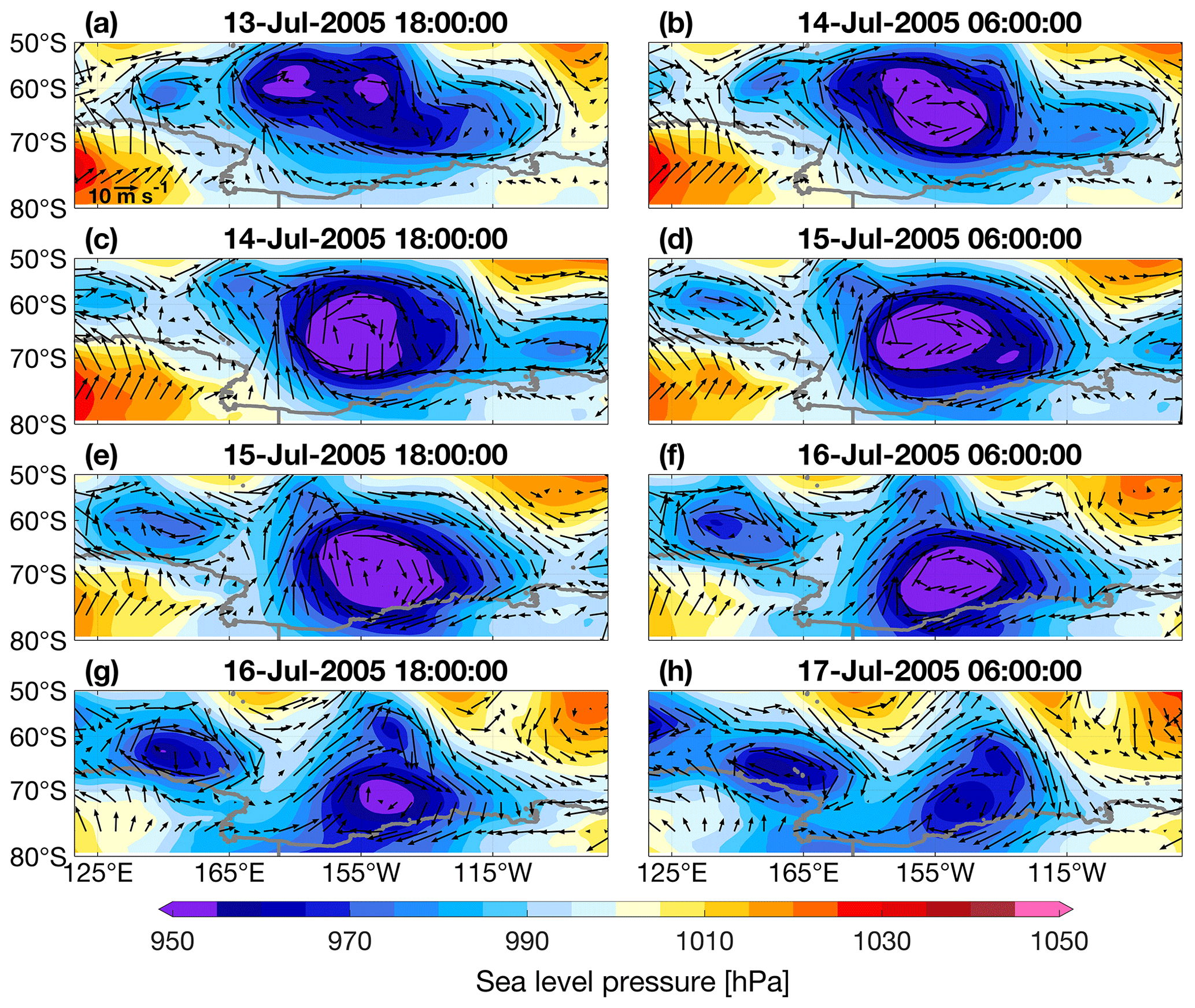
Figure 4 (a–h) Spatial distributions of 12 h average sea level pressure (colored shading) and 10 m wind vectors (black arrows) in the Ross Sea and surrounding regions over 13–17 July 2005.

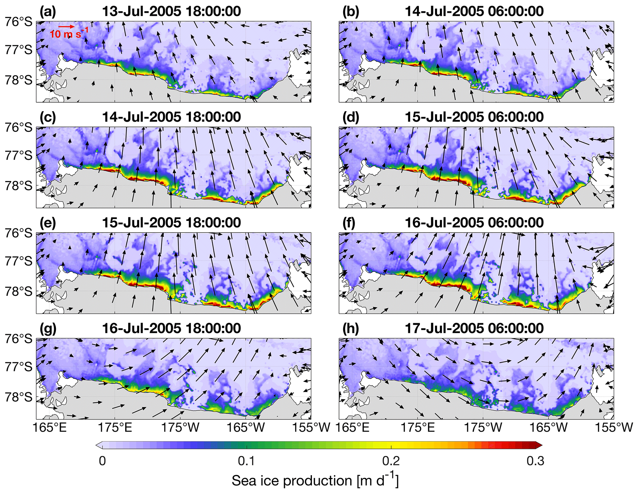
Figure 5 (a–h) Spatial distributions of 12 h average wind vectors and sea ice production (colored shading) in the Ross Ice Shelf Polynya over 13–17 July 2005.

Table 1 Comparisons of polynya-averaged sea ice production rates and HSSW properties under the normal and selected synoptic-scale and mesoscale cyclones (SYNO1, SYNO2 and MESO) for the RISP. The normal values are calculated prior to these events, from 06:00 on 13 July to 18:00 on 13 July for SYNO1, 12:00 on 16 September to 00:00 on 18 September for SYNO2, and 18:00 on 20 June to 12:00 on 21 June for MESO. The cyclone time ranges used in the calculation are consistent with those shown in Figs. 4 and 8 and Fig. S1 in the Supplement.

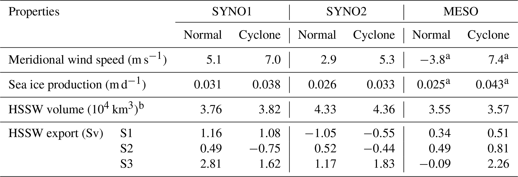
^a The calculation was conducted for the region west of 175^∘ W within the defined RISP, as the eastern region is dominated by onshore winds, resulting in no significant change in SIP.
^b The calculation was performed with a 24 h lag for synoptic-scale events and a 12 h lag for the mesoscale event respectively, based on the discovered lag time of HSSW volume response to the cyclones.

The water mass properties in the RISP region during the SYNO1 event are illustrated in Fig. 6a. Note that HSSW was mainly formed in the western section of RISP (167–176^∘ E), and fresher water accumulated from 176^∘ E to 154^∘ W (Fig. 6a), which is consistent with previous studies that observed the highest HSSW accumulation in the western sector of the Ross Sea (Jacobs et al., 1985; Budillon et al., 2003; Mathiot et al., 2012). The HSSW volume increased significantly from 18:00 on 14 July to 06:00 on 16 July (Fig. 6b), when a dramatic increase in SIP occurred in this area, accompanied by the intensification of the SYNO1 cyclone. The HSSW volume still kept increasing, indicated by the positive values for HSSW volume variability, even when SYNO1 weakened from 18:00 on 16 July to 18:00 on 19 July (Fig. 6b), so the HSSW formation could persist around 3 d after the cyclone decayed. For SYNO1, the HSSW volume increased by 0.06×10⁴ km³ compared to the value before the cyclone (Table 1). Meanwhile, the HSSW salinity presented similar features to the HSSW volume variability and reached the maximum at 18:00 on 16 July (Fig. 6c) when the cyclone had intensified for 2 d. The higher-salinity HSSW persisted for 2–3 d after the decay of the cyclone from 18:00 on 16 July to 06:00 on 19 July, and then the salinity started decreasing (Fig. 6c).

Figure 6 (a) Temperature–salinity diagram for the RISP region shown in Fig. 2a at 18:00 on 13 July 2005. The T–S dots are color-coded with longitude. The black isolines denote the neutral density contours of 28 and 28.27 kg m⁻³. The purple box shows the range of potential temperatures below −1.85 ^∘C and salinities above 34.62 psu. (b–c) Time series of panel (b) HSSW volume variability and (c) averaged HSSW salinity over the RISP region shown in Fig. 2a from 18:00 on 13 July to 06:00 on 21 July 2005. The gray shading represents the time of the SYNO1 event.

The HSSW exports across the three selected transects (S1, S2, and S3 in Fig. 1b) were calculated and related to the changes in meridional winds (Fig. 7a, b). The northward winds increased slightly from 18:00 on 13 July to 18:00 on 14 July and then turned onshore at 06:00 on 17 July (Fig. 7a, b), associated with the evolution of the SYNO1 cyclone. The export of HSSW across S1 has a significant positive correlation with the meridional wind speed (R=0.70, P=0.012), suggesting that the HSSW had stronger eastward (positive, toward RISP) transport across the meridionally directed transect S1 when the wind speed increased. The transport across the zonally directed transect S3 significantly and positively correlated with the meridional wind speed (R=0.76, P=0.004). The averaged current velocity on S1 and the averaged current velocity on S3 both have strong correlations with HSSW export (R²>0.98 and P<0.0001), suggesting that the velocity is the dominant factor regulating the export (Figs. 7a, b). Time series of HSSW export and wind speed for transect S2 are not shown as no significant correlation between these two variables was detected.

The vertical sections of neutral density and circulation along transects S1–S3 were analyzed to identify physical mechanisms behind the correlations discussed above (Fig. 7c–n). When the offshore wind speed decreased between 14 and 17 July (Fig. 7a), there was no significant change in the distribution of HSSW along S1 (Fig. 7f, i, and l). Meanwhile, there was notable change in the cross-transect current velocity: the positive (eastward) velocity in the upper layer between 76.7 and 76.5^∘ S decreased significantly, while the negative (westward) velocity in the bottom layer increased (Fig. 7f to i and l). Both features could lead to reduced eastward exports when the wind speed decreased. When the offshore wind speed increased between 06:00 and 18:00 on 13 July (Fig. 7a), changes in the cross-transect current velocity on S1 were exactly the opposite of those found during the decrease of the wind (Fig. 7c to f). For S3, the distribution of HSSW had no significant changes, while the change in velocity is much more pronounced between 178.4^∘ E and 178.7^∘ W, where the positive (northward) velocity decreased on the west side and the negative (southward) velocity increased on the east side (Fig. 7h, k, and n) when the offshore wind speed decreased (Fig. 7b), resulting in a decrease in HSSW export, which is positively correlated with the wind speed. The dynamical mechanisms for the change in currents will be discussed in Sect. 3.4. For S2, although there is no significant correlation between the HSSW export and the wind speed, the vertical distribution shows a decrease in northward export (Fig. 7d, g, j, and m).

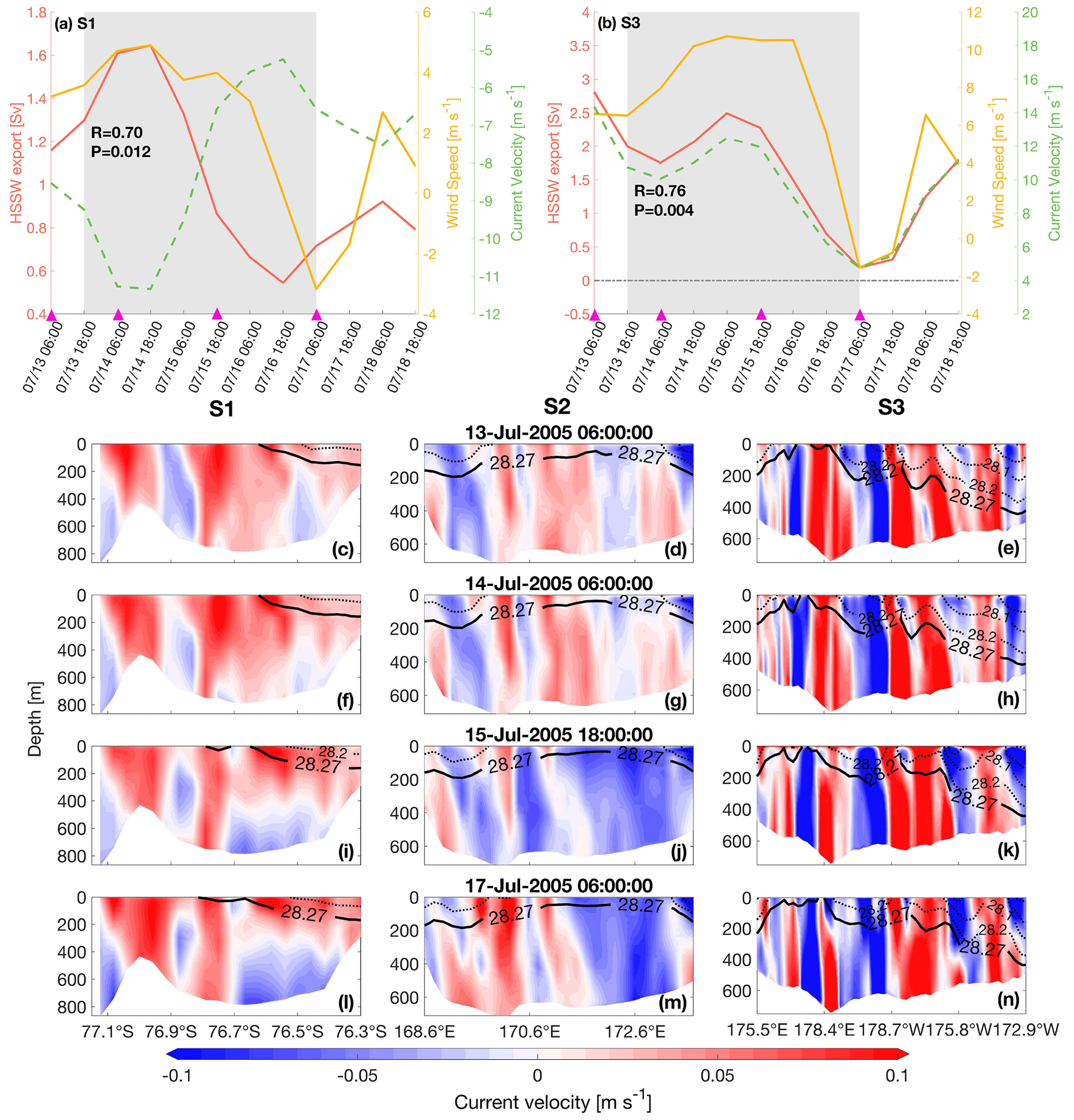
Figure 7 (a) Time series of averaged meridional winds along the S1 transect (see Fig. 1), HSSW exports across the S1, and averaged current velocity along the S1 from 06:00 on 13 July to 18:00 on 18 July 2005. The gray shading represents the time of the SYNO1 event. The correlation coefficient R and P value were calculated between the HSSW export and meridional winds. (b) Same as panel (a) but for S3. (c–n) Vertical sections of cross-transect current velocity (colored shading) and neutral density (contour lines) on (c, f, i, l) S1, (d, g, j, m) S2, and (e, h, k, n) S3 at four selected time moments (indicated by the magenta triangles in panels a and b). Positive values denote eastward currents for S1 and northward currents for S2 and S3. The bold black line indicates the neutral density contour of 28.27 kg m⁻³.

3.2.2 The SYNO2 case

The second selected synoptic-scale cyclone (SYNO2) developed from 00:00 on 18 September to 12:00 on 22 September 2014 and was located on the eastern side of the Ross Sea close to the Amundsen Sea, which is further east than the SYNO1 event (Fig. S1). The entire period of this synoptic-scale cyclone can be divided into three stages. In Stage I, the cyclone developed, and the low-pressure center expanded in all directions (Fig. S1a–d). In Stage II, the center moved eastward (Fig. S1e–g). In Stage III, the cyclone rapidly decayed (Fig. S1h–j). The spatial pattern of SIP in the RISP is displayed in Fig. S2. During Stage I, SIP increased over the entire RISP due to the strong offshore winds (Fig. S2a–d), and the increase was more pronounced on the western side of the polynya compared to the eastern side. As the cyclone entered Stage II, SIP showed opposite changes over the eastern and western sides compared to Stage I, when the offshore wind over the western polynya was still strong, but the wind over the eastern polynya had significantly turned and weakened (Fig. S2e–g). There was a notable SIP decrease over the entire RISP when the SYNO2 cyclone decayed in Stage III (Fig. S2h–j). Similar to SYNO1, SIP quickly responded to the variation of winds over the entire RISP. For the SYNO2 event, the area-averaged wind speed increased by almost 2 times compared to before the cyclone's arrival, reaching 5.3 m s⁻¹. The area-averaged SIP showed an increase of about 27 %, reaching 0.033 m d⁻¹ (Table 1).

For the water mass response, HSSW volume variability in the RISP increased significantly until 00:00 on 21 September and then maintained positive values for at least 60 h (Fig. S3a). The salinity of newly formed HSSW increased to 34.84 psu at 00:00 on 21 September after Stages I and II of SYNO2 (Fig. S3b). Afterwards, the volume and salinity of HSSW kept increasing for 36 h when the coastal SIP was already decreasing (Figs. S2 and S3). Therefore, both events (SYNO1 and SYNO2) revealed persistent impacts of cyclones on the HSSW formation, even after these weather systems had decayed. The HSSW exports across the three transects (S1–S3) were calculated during the SYNO2 event but are not shown as the meridional winds and the HSSW exports across S1 and S2 did not correlate. For S3 on the other hand, there was a significant but weak positive correlation between the meridional wind speed and the HSSW export 12 h later (R=0.53, P=0.042). The reason for the weaker correlations between HSSW export and wind speed over SYNO2 might be related to the lower wind speed in RISP compared to the SYNO1 event (5.3 m s⁻¹ for SYNO2 and 7.0 m s⁻¹ for SYNO1, shown in Table 1), resulting from the faraway cyclone center located in the Amundsen Sea. Additionally, other factors (such as the circulations of ice shelf basal melting water) could regulate the HSSW exports significantly. As shown in Table 1, there was an increase in the HSSW volume during SYNO2, being 0.03×10⁴ km³ larger than the value before the event. The HSSW export across S3 increased about 56 % when the wind speed increased from 2.9 to 5.3 m s⁻¹, while the magnitude of export across S1 and S2 decreased.

Figure 8 (a–h) Spatial distributions of 6 h average sea level pressure (colored shading) and 10 m wind vectors (black arrow) in the Ross Sea and surrounding regions over 21–23 June 2005.

3.3 The MESO case

The selected mesoscale cyclone event was present around RISP from 12:00 on 21 June to 06:00 on 23 June 2005, which is associated with the synoptic cyclone being located farther northwest of the Ross Sea (not shown). The formation of this MESO case is consistent with earlier studies that demonstrate that the small synoptic systems could merge into mesoscale cyclones (Carrasco and Bromwich, 1993; Uotila et al., 2009). From the patterns of sea level pressure and wind vectors (Fig. 8), the center of the cyclone was located in the middle of the Ross Sea (Fig. 8c–f), and the horizontal length scale ranged from 500–1000 km. The trajectory of this cyclone was located in the area of high track densities of the Ross Sea (Fig. 3b), suggesting that it is a typical mesoscale cyclone for this region. An enlargement of the wind field is shown in Fig. 9 on top of the SIP field. During the initial stage of MESO (Fig. 9a, b), the entire RISP was influenced by the southern branch of the cyclone and the prevailing alongshore wind. There was little variation in SIP, as the offshore component of wind did not significantly change. As the center of the cyclone moved south and approached RIS (Fig. 8c–e), the western and eastern sections of RISP were respectively affected by the southerly and northerly winds induced by MESO. As a result of the enhanced offshore winds, SIP in the western section increased rapidly to over 0.3 m d⁻¹ (Fig. 9c–e). When the cyclone center moved further south onto the ice shelf and the cyclone winds weakened (Fig. 8f–h), there was a notable decrease of SIP, suggesting that SIP responds quickly to the winds (Fig. 9f–h). In contrast to the western polynya, SIP in the eastern polynya presented a slight decrease during MESO (Fig. 9a–e), which was due to the onshore winds generated by MESO that shrunk the polynya. The response of SIP in RISP was instantaneous during these selected cyclones, which is consistent with the variation for SIP during typical strong wind events in East Antarctic coastal polynyas including the Prydz Bay and Shackleton polynyas (Wang et al., 2021). During MESO, area-averaged SIP increased by 72 % compared to before the cyclone's arrival (Table 1), reaching 0.043 m d⁻¹, while the meridional wind speed rose from −3.8 to 7.4 m s⁻¹. Thompson et al. (2020) proposed that the intensity of ice production could rise up to 1.1 m d⁻¹ during the events when the wind speeds exceeded 20 m s⁻¹ in TNB, which was calculated from the salt budget using conductivity–temperature–depth (CTD) profiles. Meanwhile, the maximum SIP rate in the RISP during MESO was 1.2 m d⁻¹ in our study when the wind speed was around 15 m s⁻¹, which is just slightly different from the value in TNB. The air temperatures for both TNB and RISP were below −25 ^∘C. Differences in topography and location between the RISP and TNB could lead to such slight differences in atmospheric and hydrological conditions.

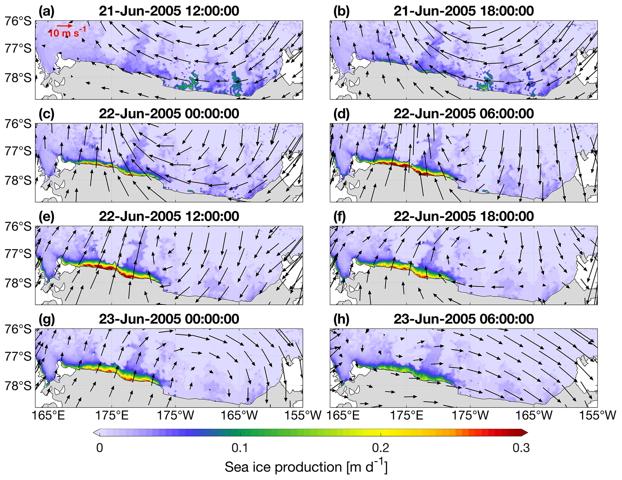
Figure 9 (a–h) Spatial distributions of 6 h average wind vectors and sea ice production (colored shading) near the Ross Ice Shelf Polynya over 21–23 June 2005.

Figure 10a represents a continuous increase for HSSW volume over MESO until 18:00 on 23 June when the cyclone already disappeared. Furthermore, it can be seen from Fig. 10b that the averaged HSSW salinity began increasing on late 22 June, responding to the increase in SIP (Fig. 9a–f). The volume and salinity of HSSW increased persistently even during the cyclone decay when SIP was already decreasing from 23 June (Figs. 9g–h and 11), which suggests that the response of the HSSW formation to a mesoscale cyclone could persist for 12–18 h, which is a comparable timescale to synoptic cyclone events but with a shorter time lag. The mean HSSW volume during MESO increased slightly by 0.02×10⁴ km³ compared to the volume before it. This is much smaller than changes under the synoptic cyclones SYNO1 and SYNO2 (Table 1). This difference is likely related to different spatial scales of cyclones. During MESO, only the western part of RISP was dominated by offshore winds due to the smaller spatial extent of the mesoscale cyclone, which resulted in a smaller region for HSSW production than that under synoptic-scale cyclones during SYNO1 and SYNO2.

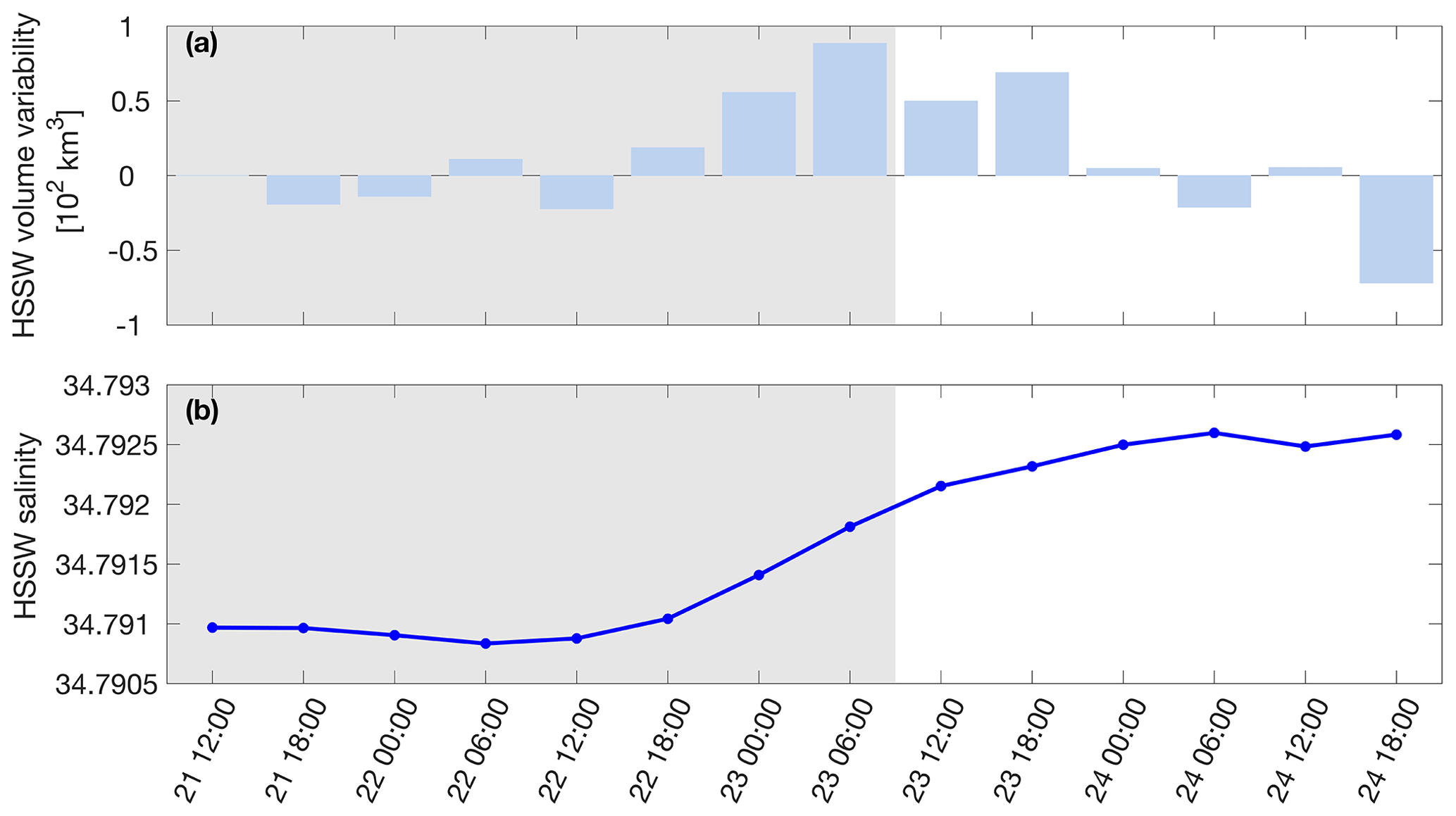
Figure 10 Time series of (a) HSSW volume variability and (b) averaged HSSW salinity over the RISP region shown in Fig. 2a from 12:00 on 21 June to 18:00 on 24 June 2005. The gray shading represents the time of the MESO event.

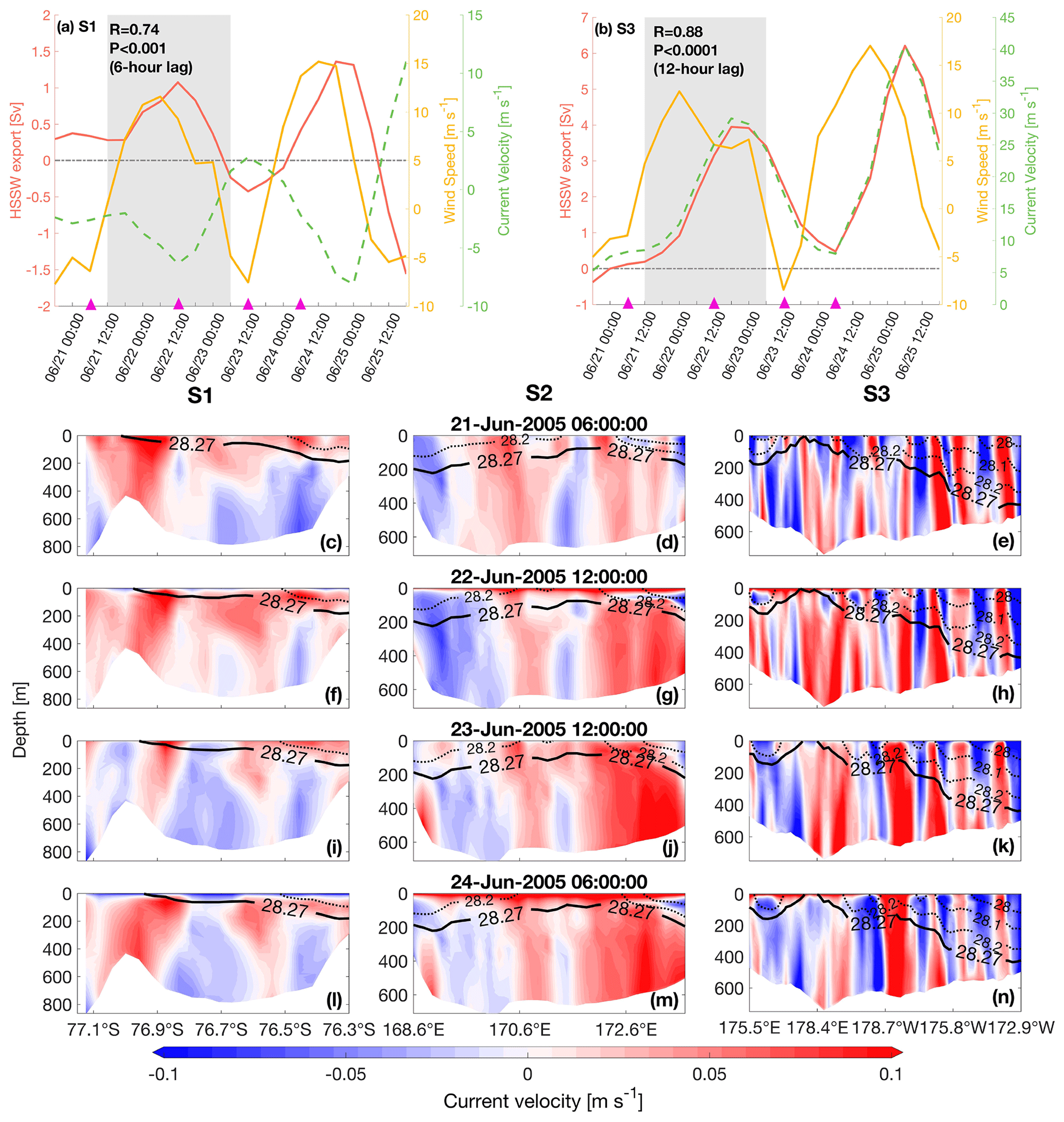
Figure 11 (a) Time series of averaged meridional winds along the S1 transect (see Fig. 1), HSSW exports across the S1, and averaged current velocity along the S1 from 18:00 on 20 June to 18:00 on 25 June 2005. The gray shading represents the time of the MESO event. The correlation coefficient R and P value were calculated between the HSSW export and meridional winds. (b) Same as panel (a) but for S3. (c–n) Vertical sections of cross-transect current velocity (colored shading) and neutral density (contour lines) on (c, f, i, l) S1, (d, g, j, m) S2, and (e, h, k, n) S3 at four selected time moments (indicated by the magenta triangles in panels a and b). Positive values denote eastward currents for S1 and northward currents for S2 and S3. The bold black contour line indicates the neutral density contour of 28.27 kg m⁻³.

The HSSW exports across transects S1–S3 over the period of the mesoscale cyclone MESO are shown in Fig. 11. To better investigate the relationship between the HSSW export and the cyclone event, distributions of wind vectors and sea level pressure were examined for about 2 d after the end of MESO (i.e., until 25 June). The two maxima of wind speed time series are associated with two consecutive mesoscale cyclones (Fig. 11a–b). For transect S1, there is a significant, positive correlation between the meridional wind speed and HSSW export, with a 6 h lag from 21 to 25 June (R=0.74, P<0.001) (Fig. 11a). Furthermore, relationships of wind speed and HSSW export across S1 and S3 are similar. The HSSW export across S3 is significantly and positively related to the wind speed, with a 12 h lag (R=0.88, P<0.0001). The export across S2 has a positive correlation with wind speed though weaker compared to S1 (R=0.41 and P=0.07, not shown). By examining the ocean currents near S2, a northward flow originated around 79^∘ S which is located at the RIS (Fig. S7e, h, k and f, i, l) was observed, and the weaker correlation between HSSW export and wind speed might be associated with local ice shelf circulations. For transects S1 and S3, the current velocity is significantly correlated with the HSSW export with no lag (R²>0.99 and P<0.0001, Fig. 11a–b), resembling the SYNO1 case. As there are lag correlations between wind speed and current velocity both for S1 and S3, such a relationship can explain why the HSSW export also exhibited lag responses to the wind speed. The HSSW export increased by 50 % across S1 and increased by 2.35 Sv across S3 when the offshore wind speed increased from −3.8 to 7.4 m s⁻¹ compared to the values before MESO (Table 1). Vertical sections for ocean currents and potential density are presented in Fig. 11c–n. For S1, negative (westward) transport was observed in the upper 50 m (Fig. 11f and l) when offshore wind speed became stronger, which can be interpreted as enhanced westward Ekman transport (Fig. 11a). Consistent with the features found under synoptic-scale cyclones, the major factor inducing the change in HSSW export across S1 is the current velocity change below 50 m: the positive (eastward) velocity increased between 77.1–76.9 and 76.7–76.5^∘ S, corresponding to the increase of wind speed, and the negative (westward) velocity decreased in the central section between 76.9 and 76.7^∘ S (Fig. 11c to f and i to l), ultimately leading to a positive correlation between the wind speed and the HSSW export. For S2, the most eminent feature is that the export of HSSW is mainly concentrated on the eastern side of the section (Fig. 11d, g, j, and m), which originates from the RIS region. For S3, there was no significant change in HSSW compared to the change in current velocity. The sharp change in current velocity over 178.4^∘ E–178.7^∘ W dominates the variation of HSSW export (Figs. 11e, h, k, and n).

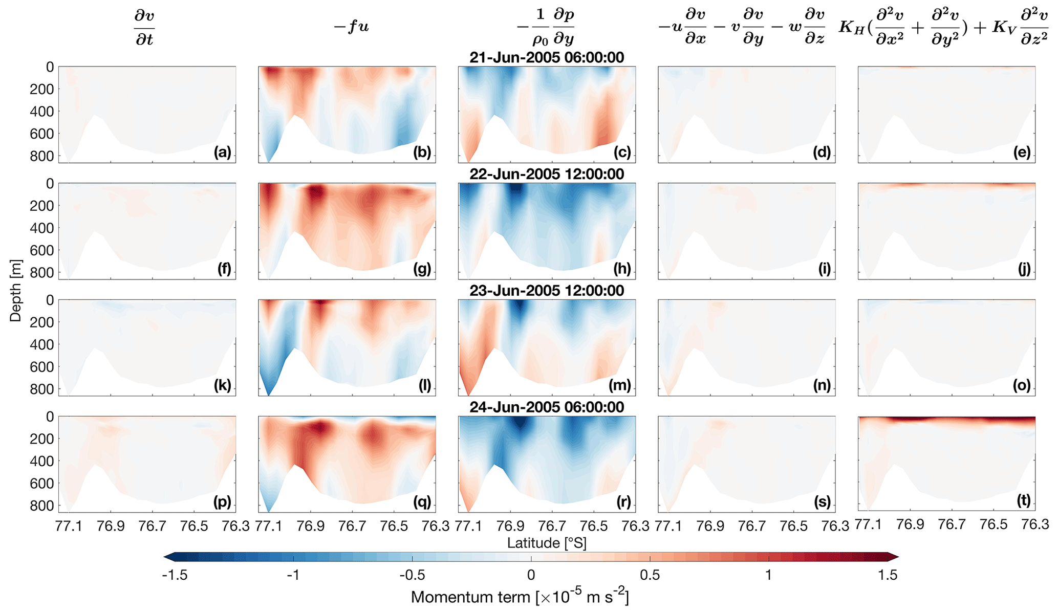
Figure 12 Vertical sections of the momentum equation terms (Eq. 2) along S1 at four selected time moments during the MESO event (indicated by the magenta triangles in Fig. 11a and b): (a, f, k, p) local acceleration, (b, g, l, q) Coriolis acceleration, (c, h, m, r) pressure gradient, (d, i, n, s) nonlinear advection, and (e, j, o, t) eddy viscosity in the across-ice-shelf momentum budget.

3.4 Potential mechanisms for the HSSW export variations

As illustrated in Sect. 3.2 and 3.3, for both SYNO1 and MESO, the HSSW export across S1 and S3 was positively correlated with the meridional wind speed (Figs. 7a–b and 11a–b). These relationships also exist over the longer time periods of June–September in 2005 and 2014 but with relatively lower correlation coefficients (R=0.27 and P<0.0001 with a lag of 6–12 h for S1 and R=0.42 and P<0.0001 with a 12 h lag for S3). Meanwhile, it is clear that the current velocity is the dominant factor in modulating the HSSW export change compared to the HSSW volume for both S1 and S3 (Figs. 7 and 11). Then, to elucidate the dynamical control for the current variations, we examined the momentum budgets for S1 and S3 in SYNO1 and MESO. For SYNO1 (Figs. S4 and S5), the momentum balance presents similar results to those of MESO. The vertical sections of momentum terms on S1 and S3 in MESO are displayed in the across-ice-shelf (Fig. 12) and along-ice-shelf (Fig. 13) directions respectively. For both directions, the momentum budgets were dominated by the Coriolis acceleration and pressure gradient terms, and the other terms were an order of magnitude smaller (Figs. 12 and 13). As such, the flows across these transects (in the along-shelf direction for S1 and the cross-shelf direction for S3) were primarily geostrophic (Figs. 12 and 13).

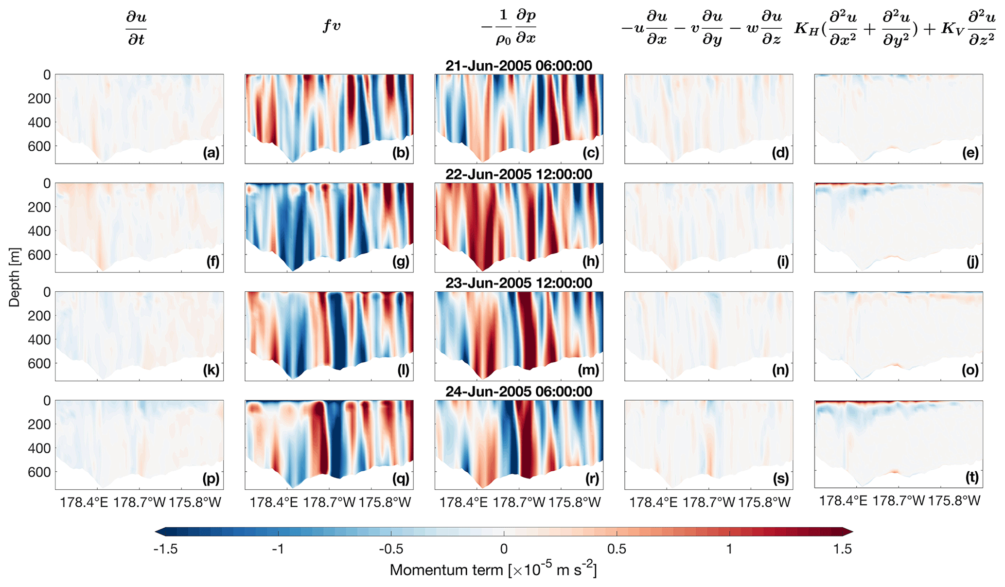
Figure 13 Vertical sections of the momentum equation terms (Eq. 1) along S3 at four selected time moments during the MESO event (indicated by the magenta triangles in Fig. 11a and b): (a, f, k, p) local acceleration, (b, g, l, q) Coriolis acceleration, (c, h, m, r) pressure gradient force, (d, i, n, s) nonlinear advection, and (e, j, o, t) eddy viscosity in the along-ice-shelf momentum budget.

For S1, there were two zones (77.1–76.9 and 76.7–76.5^∘ S) where the current velocity changed notably (Fig. 11c, f, i, and l) during MESO, corresponding to the change in the Coriolis (Fig. 12b, g, l, and q) term, which was associated with the change in the pressure gradient (Fig. 12c, h, m, and r) term. We then examined the spatial distribution of sea surface elevation over the Ross Sea (Fig. 14), where negative values near the RIS close to S1 existed persistently. Such distribution resulted in southward (negative) pressure gradient force due to sea surface differences over S1, leading to an eastward geostrophic flow across S1. When the wind speed increased at 12:00 on 22 June and 06:00 on 24 June (Fig. 11a), the pressure gradient force was larger than that under lower wind speeds (compare Fig. 14b and d to a and c). These features suggest that the increased offshore winds induced intensified westward Ekman transport in the upper layer in the area bounded by 74–76.5^∘ S and 163–176^∘ E just north of S1 (marked by the blue box in Fig. 15d and j), eventually resulting in the higher sea surface in this region (Fig. 14b and d). Meanwhile, the relatively strong vertical shear in the upper layer suggests that the Ekman transport could dominate on top of the interior geostrophic current (Fig. 12j and t), which contributed to the variation of sea surface elevation over S1. However, near the RIS between 163 and 176^∘ E, where offshore winds also prevailed, the increase in surface elevation (i.e., the enhanced westward Ekman transport) could barely be detected (Fig. 15). After examining the horizontal pattern of currents over the Ross Sea, we found a southeastward flow across S1 located north of the Ross Island (within the green boxed area near S1 in Fig. 15), which can also be detected in Fig. 14, suggesting that it can be regarded as the barotropic flow resulting from sea surface change. Furthermore, this southeastward current further flowed southward below the RIS in the deeper layer (Fig. 15b, c, e, f, h, i, k and l), and the zonal and meridional components of this southeast flow can be observed more clearly in Figs. S6 and S7 respectively. Previous studies showed that there is an HSSW inflow underneath the RIS through the Ross Island (Assmann et al., 2003; Budillon et al., 2003), which could advect more than 10 % of HSSW to the southern part of RIS and intensify continuously over the winter (Jendersie et al., 2018). Therefore, we speculate this southward inflow is one of the reasons for the persistent low sea surface elevation in the area close to the RIS (Fig. 14). In addition, we further examined the barotropic and baroclinic components for this geostrophic flow along S1 (Figs. S8 and S9). The positive (eastward) velocity in the upper layer in the area bounded by 77.1–76.9 and 76.7–76.5^∘ S (Fig. 11c, f, i, and l) is regulated by the barotropic current (Fig. S8a, d, g, and j), while the negative (westward) velocity in the deeper layer (Fig. 11c, f, i, and l) is related to the baroclinic component resulting from the density differences across S1 (Fig. S9a, d, g, and j).

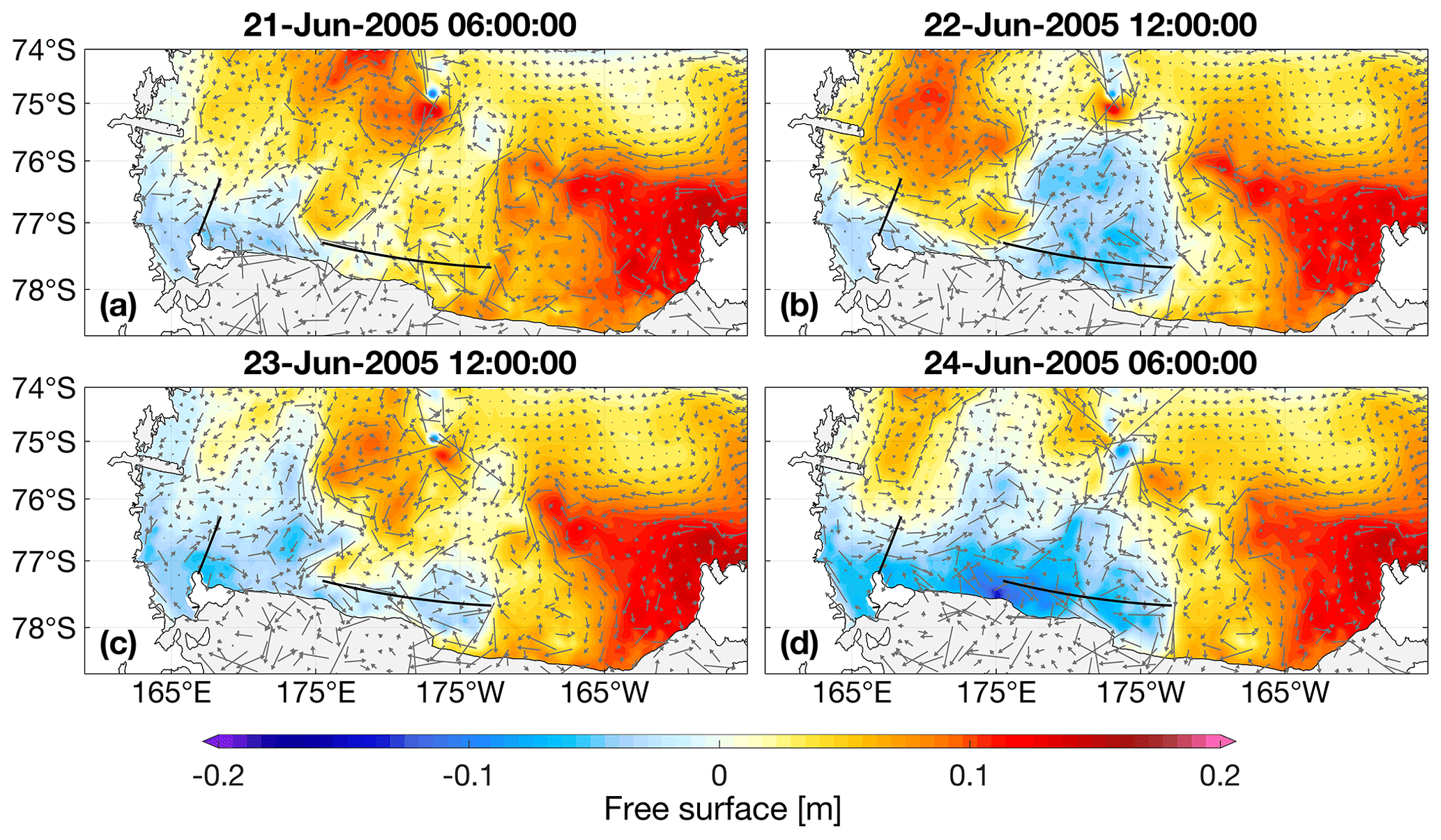
Figure 14 (a–d) Spatial distributions of free surface (colored shading) and barotropic geostrophic currents (gray arrow) in the Ross Sea region at four selected time moments of MESO (indicated by the magenta triangles in Fig. 11a and b). The black lines indicate the S1 and S3 section.

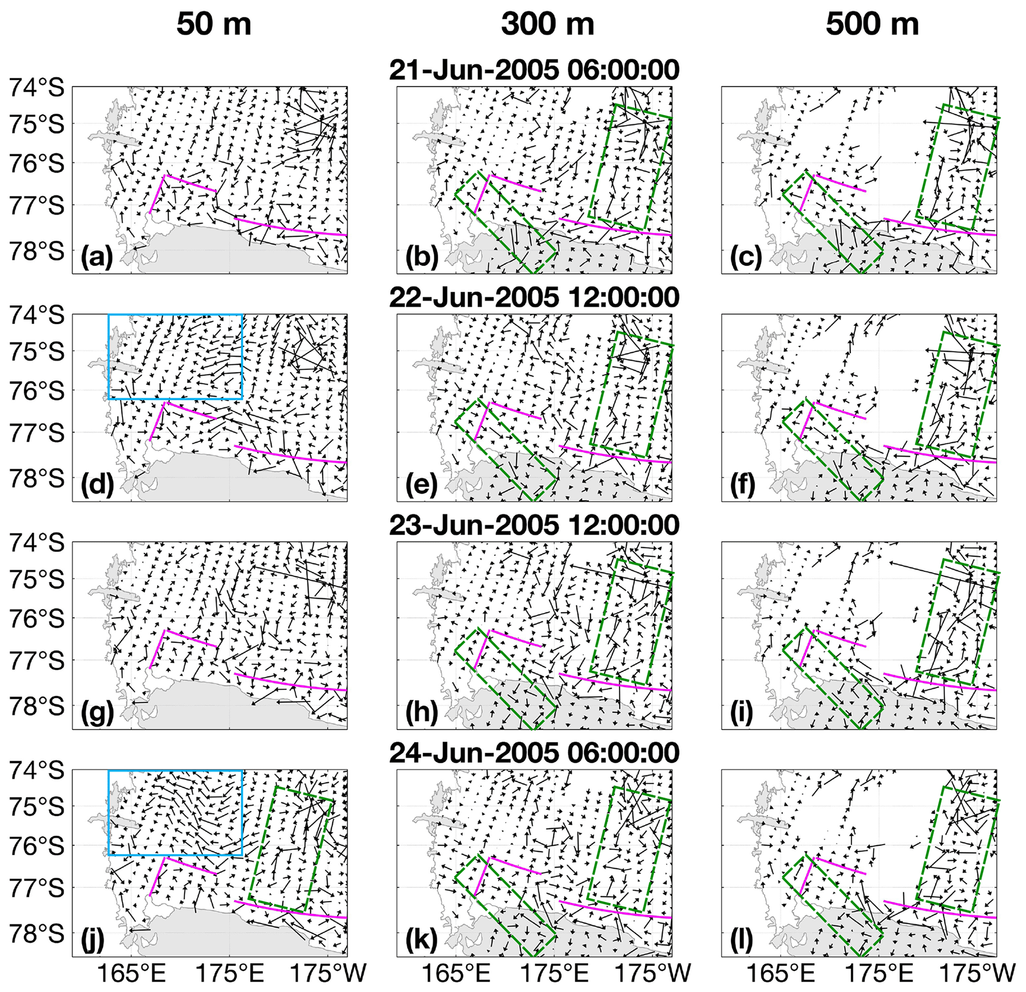
Figure 15 Spatial distributions of ocean currents at the depth of (a, d, g, j) 50 m, (b, e, h, k) 300 m, and (c, f, i, l) 500 m at four selected time points (06:00 on 21 June, 12:00 on 22 June, 12:00 on 23 June, and 06:00 on 24 June). The magenta lines are the S1, S2, and S3 sections defined in Fig. 1b. The blue boxes indicate the areas where westward Ekman transport is observed. The green boxes near S1 and S3 indicate the areas where southeastward and outward (northward) flows are present respectively.

Along S3, the western section (178.4^∘ E –178.7^∘ W) with a considerable velocity change (Fig. 11e, h, k, and n) dominated the variation of HSSW export. Meanwhile, an outward (northward) flow can be seen clearly over the Glomar Challenger Trough across the western section (marked by the green box near S3 in Fig. 15). From the distribution of sea surface elevation, it is noted that the elevation was lower when the wind speed increased over the Glomar Challenger Trough (Fig. 14b and d), which might be associated with the divergent Ekman transport caused by the cyclone. Such a divergent pattern would generate a positive (eastward) pressure gradient force over the western section of S3, which drove northward barotropic geostrophic flows associated with the HSSW transport occupying this area (Fig. 11e, h, k, and n). Such barotropic currents could be identified on S3 in Fig. S8. Meanwhile, the baroclinic geostrophic flow also plays an important role in HSSW export across S3 (Fig. S9c, f, i, and l). Therefore, the northward flow is regulated by both barotropic and baroclinic components. These features for MESO are consistent with those we found for SYNO1 (Figs. S10 and S11).

3.5 Lag time for HSSW formation and export

The HSSW formation in the RISP demonstrated a near-instantaneous response to the wind change during the synoptic-scale and mesoscale cyclone events (Figs. 6, S3, and 10), which could persist for 12–60 h after the passage of the cyclones. These features are somewhat different from the HSSW response over the East Antarctica coastal polynyas as proposed by Wang et al. (2021), which elucidates a lag response of 10–15 d for the HSSW formation to strong wind events in the Prydz Bay and Shackleton polynyas. Such discrepancy might be related to the polynya extent and local circulations. The RISP has been regarded as the highest ice production region among the major 13 Antarctic coastal polynyas (Tamura et al., 2008), suggesting intensified brine rejection that will result in faster production of HSSW. Another factor might be the local circulation system like the outflow of basal melting water and the local gyre over these coastal regions. Herraiz-Borreguero et al. (2016) highlight the role of ice shelf water in controlling the HSSW formation rate and its thermohaline properties in East Antarctica. Formation of HSSW could be hindered by the freshwater input from ice shelves (Williams et al., 2016). Meanwhile, the increased freshwater from ice shelf melting could reduce the transport of circumpolar deep water onto the continental shelf region (Dinniman et al., 2018), which can further affect the formation of dense shelf water.

The HSSW exports across S1 and S3 were positively correlated with wind speed over MESO with a 6 and 12 h lag respectively (Fig. 11a–b). Furthermore, as mentioned before, such a lag relationship between wind and HSSW was robust over June–September in 2005 and 2014, while the lag time could vary between 6 and 12 h. Mathiot et al. (2012) documented a 6-month time lag between the HSSW formation in polynyas (TNB and RISP) and the HSSW transport across the topographic sills in the Ross Sea; i.e., the maximum HSSW transport occurred during summer (February/March), while the maximum of polynya activity occurs in winter (August/September). The defined sections across the Drygalski Trough and the Joides Trough in their study were located around 74^∘ S, which is about 330 km further north than the sections we selected. This study provided a baseline for us to estimate the timescale for the cyclone-induced sea ice and HSSW change to influence bottom water properties at the slope. Generally, the lag time between the changes in wind and HSSW exports is highly dependent on the locations of chosen transects and the spreading rate of HSSW.

4 Conclusions

This study investigated the response of sea ice and HSSW formation and export in the Ross Ice Shelf Polynya to mesoscale and synoptic-scale cyclones based on a coupled ocean–sea ice–ice shelf Ross Sea model. For synoptic-scale cyclones, two representative events were selected, and for mesoscale cyclones one representative event was selected. When synoptic-scale cyclones with spatial size over 1000 km prevailed over this region, the entire RISP was dominated by strong offshore winds, which resulted in increased SIP rates in the entire RISP, while during the passage of mesoscale cyclones with radii less than 1000 km, SIP increased rapidly over the western side of RISP but decreased over the eastern side of RISP, due to changes in the offshore winds associated with the cyclonic wind field. SIP instantaneously responded to the wind change over the RISP under both the synoptic-scale and mesoscale cyclones. Enhanced HSSW formation was detected when there was a notable increase of SIP in RISP, mainly in the western side of RISP, and could persist for 12–60 h after the passage of the cyclones. The main differences in the response of HSSW formation to the synoptic-scale and mesoscale cyclones lie in the persistence time of high-salinity signals after the cyclone decayed. For the two synoptic-scale cyclones, the increase in HSSW formation persisted for about 2–3 d, while the response of HSSW formation to the mesoscale cyclone had a shorter lag of about 12–18 h. The HSSW exports across the transects over the Drygalski Trough (S1) and the Glomar Challenger Trough (S3) were positively correlated with the meridional wind. The variations of the HSSW export across S1 and S3 were mainly regulated by the geostrophic currents. Pressure gradients driving the geostrophic currents were related to barotropic gradients in sea surface caused by wind-induced Ekman transport and the baroclinic gradients resulting from the density differences. However, there might be other factors that affected the hydrography near the Ross Island along the S1 transect. For instance, the melting beneath the RIS and the intrusion of the circumpolar deep water have impacts on currents in this region, which deserves future investigations to reveal the different responses for S1 and S3. In addition, tides could further modulate the export and volume of HSSW in this region (Padman et al., 2009; Wang et al., 2013), and such effects should be considered by using models including the tides in the future.