Geometric controls of tidewater glacier dynamics

Retreat of marine outlet glaciers often initiates depletion of inland ice through dynamic adjustments of the upstream glacier. The local topography of a fjord may promote or inhibit such retreat, and therefore fjord geometry constitutes a critical control on ice sheet mass balance. To quantify the processes of ice–topography interactions and enhance the understanding of the dynamics involved, we analyze a multitude of topographic fjord settings and scenarios using the Ice-sheet and Sea-level System Model (ISSM). We systematically study glacier retreat through a variety of artificial fjord geometries and quantify the modeled dynamics directly in relation to topographic features. We find that retreat in an upstream-widening or upstream-deepening fjord does not necessarily promote retreat, as suggested by previous studies. Conversely, it may stabilize a glacier because converging ice flow towards a constriction enhances lateral and basal shear stress gradients. An upstream-narrowing or upstream-shoaling fjord, in turn, may promote retreat since fjord walls or bed provide little stability to the glacier where ice flow diverges. Furthermore, we identify distinct quantitative relationships directly linking grounding line discharge and retreat rate to fjord topography and transfer these results to a long-term study of the retreat of Jakobshavn Isbræ. These findings offer new perspectives on ice–topography interactions and give guidance to an ad hoc assessment of future topographically induced ice loss based on knowledge of the upstream fjord geometry.

1 Introduction

Rates of ice discharge from the Greenland Ice Sheet are likely to exceed their Holocene (last 12 000 yr) maxima this century (Briner et al., 2020; Kajanto et al., 2020), and parts of Antarctica are on the brink of irreversible mass loss (Garbe et al., 2020). Consequently, major natural and societal challenges related to changes in the terrestrial cryosphere of the high latitudes lay ahead. An advanced understanding of the underlying processes of ice loss is paramount for fact-based decision-making (Oppenheimer et al., 2019).

About half of the current mass loss over Greenland (30 % to 70 %) is due to dynamic ice discharge related to thinning, speed-up and increased calving of outlet glaciers (Nick et al., 2009; Felikson et al., 2017; Haubner et al., 2018; Mouginot et al., 2019; King et al., 2020). In Antarctica, dynamic instability of the West Antarctic Ice Sheet is considered a major driver of future sea-level rise (Pattyn and Morlighem, 2020), but there is also emerging evidence of changes in ice dynamics at some glaciers in East Antarctica (Brancato et al., 2020; Miles et al., 2020). While outlet glaciers therefore are critical to ice sheet mass balance and associated sea-level rise, considerable knowledge gaps on the processes governing their dynamics still exist.

Despite the general warming trend observed over the recent decades, we do not observe an overall synchronous pattern in outlet glacier evolution. This is clear for various settings in the Arctic, such as in Greenland (Warren and Glasser, 1992; Carr et al., 2013; Bunce et al., 2018; Catania et al., 2018), Svalbard (Schuler et al., 2020), Novaya Zemlya (Carr et al., 2014) and North America (McNabb and Hock, 2014) as well as in Antarctica (Pattyn and Morlighem, 2020). Even adjacent glaciers with similar climatic and oceanic conditions can show strongly different behavior (Carr et al., 2013; Catania et al., 2018; Bunce et al., 2018). The main proposed explanation is that differing bathymetry and glacier geometry significantly modulate glacier response to climate over a range of timescales (Warren and Glasser, 1992; Briner et al., 2009; Jamieson et al., 2012; Åkesson et al., 2018a; Catania et al., 2018). Broadly, there is a consensus that wide and deep parts of a fjord promote retreat, while narrow and shallow areas tend to stabilize glacier termini. Moreover, kinematic wave theory indicates that the upstream propagation of a thinning signal is heavily influenced by bed topography (Felikson et al., 2017, 2021). Modeling of idealized settings (Enderlin et al., 2013; Åkesson et al., 2018b) and theoretical studies based on analytical calculations and numerical experiments further emphasize the potential of fjord geometry to modulate glacier retreat (Weertman, 1974; Raymond, 1996; Vieli et al., 2001; Schoof, 2007; Pfeffer, 2007; Gudmundsson et al., 2012; Gudmundsson, 2013).

It is therefore critical to advance our understanding of the influence of fjord geometry on glacier retreat to accurately predict sea-level rise, especially when extrapolating observations of a few well-monitored glaciers to those less studied (Nick et al., 2009). This knowledge is also pivotal to correctly infer past climate signals from glacier proximal landforms because their formation may have been influenced by fjord topography and may not necessarily have been in equilibrium with the prevailing climate (Åkesson et al., 2018b; Steiger et al., 2018).

The most important suggested mechanisms behind geometric control of glacier retreat are (1) friction, with glaciers in narrow fjords and grounded well above flotation being stabilized by fjord geometry, while the opposite is the case for glaciers in wide fjords and close to flotation (Raymond, 1996; Pfeffer, 2007; Enderlin et al., 2013; Åkesson et al., 2018b) (buttressing and lateral shear between an ice shelf and nearby islands and/or fjord walls can be an important factor as well; Gudmundsson et al., 2012; Gudmundsson, 2013; Jamieson et al., 2012, 2014); (2) area exposed to ocean melt, where a wider or deeper fjord induces a larger cumulative melt flux (Straneo et al., 2013; Åkesson et al., 2018b); and (3) the marine ice sheet instability (MISI), which is a feedback mechanism between increasing driving stress with increasing ice thickness at the grounding line (GL), where inland-sloping (retrograde) beds lead to self-accelerating ice loss (Weertman, 1974; Schoof, 2007).

While the main controls of ice–topography interactions are known, a quantitative understanding is still largely missing, especially on timescales beyond a few decades. In this context, in situ observations of ice dynamics do not cover the full spectrum of ice–topography interactions because they are limited in space and time. While remotely sensed observations of ice dynamics over the past decades exist, the recent retreat in Greenland and elsewhere over this period is too short to allow for a complete assessment of geometry–glacier interactions (Carr et al., 2013; Catania et al., 2018; Bunce et al., 2018). In contrast, on paleo-timescales, retreat has occurred over large distances, but the temporal resolution of geomorphological studies is limited by the available geological data, and key information is missing to discern different drivers of glacier retreat (Briner et al., 2009; Åkesson et al., 2020). Meanwhile, numerical studies that can address these issues have so far mostly used width- and depth-integrated flow line models, which carry many assumptions that do not hold in some settings (Nick et al., 2009; Enderlin et al., 2013; Åkesson et al., 2018b; Steiger et al., 2018). In particular, they parameterize or do not account for factors that are thought to be instrumental to explain ice–topography interactions, such as lateral drag, across-flow variations in glacier characteristics and viscosity changes due to variations in ice temperature. The latter, for instance, was found to be key to explain Jakobshavn Isbræ's recent retreat (Bondzio et al., 2017).

Here, we use a numerical ice-flow model resolving two horizontal dimensions; we include a suite of 21 experiments and present a systematic approach to compare the relative importance of basal and lateral fjord topography. This setup allows the assessment of how fjord topography controls glacier retreat on interannual to centennial timescales. We hypothesize that there are quantifiable relationships between glacier retreat and topography that apply to a wide range of glaciological settings. Such general relationships would yield substantial predictive power for a broad assessment of expected future outlet glacier retreat.

We create a large ensemble of artificial fjords that include geometric features (referred to as “perturbations” in the following) typically found in glacial fjords, such as sills and overdeepenings (referred to as “bumps” and “depressions”, respectively; together “basal perturbations”) as well as narrow and wide fjord sections (referred to as “bottlenecks” and “embayments”, respectively; together “lateral perturbations”). We then force synthetic glaciers to retreat through this variety of fjords by increasing ocean-induced melt rates and assess key retreat metrics such as the grounding line retreat rate. The ice dynamics of each simulation are compared and quantitatively linked to the characteristics of the respective fjord geometry. Finally, we investigate whether the retreat dynamics and ice–topography interactions are transferable from the idealized setup to a long-term study on Jakobshavn Isbræ in western Greenland.

2 Methods

2.1 Ice sheet model

We use the Ice-sheet and Sea-level System Model (ISSM; Larour et al., 2012) with the shallow-shelf approximation (SSA; Morland, 1987; MacAyeal, 1989). A discussion on the appropriateness of this approximation compared to a full-Stokes model is provided in Sect. 4.2. Our domain is rectangular (80 km × 10 km), with x and y representing the along-flow and across-flow coordinates, respectively (Fig. 1a). We create an unstructured mesh with a fixed resolution of 100 m close to the GL, comparable to other high-resolution studies of Greenlandic fjords (e.g., Morlighem et al., 2016, 2019). The temporal resolution is set to Δt=0.01 yr (3.65 d) to satisfy the Courant–Friedrichs–Levy condition (Courant et al., 1928). We apply a subelement GL migration scheme (Seroussi et al., 2014) and enable a moving calving front with the level-set method (Bondzio et al., 2016). We use a thermal model (Larour et al., 2012) to constrain the ice rheology parameter, B, based on the temperature-dependent relationship from Cuffey and Paterson (2010). The spin-up ice temperature is −5 ^∘C, representative of conditions in southern and central Greenland and the southern Fennoscandian Ice Sheet (Nick et al., 2013; Åkesson et al., 2018a). To simulate calving, a von Mises law is used (Morlighem et al., 2016), where the calving rate c is given as

$$\begin{array}{}\text{(1)}& c=\left|\right|\mathit{v}\left|\right|{\displaystyle \frac{\stackrel{\mathrm{̃}}{\mathit{\sigma }}}{{\mathit{\sigma }}_{max}}},\end{array}$$

where v is the velocity vector, $\stackrel{\mathrm{̃}}{\mathit{\sigma }}$ is a scalar quantity representing the tensile stress at the ice front, and σ_max is a stress threshold. This formulation, demonstrated to perform well in Greenlandic fjords (Choi et al., 2018), means that ice front retreat occurs when the tensile stress at the glacier front exceeds a fixed threshold; σ_max generally needs to be determined experimentally for studies on real-world glaciers. Here we fix σ_max to 1 MPa for grounded ice and 200 kPa for floating ice. These values yield a representative setup and are within the range suggested for Greenland outlet glaciers (Morlighem et al., 2016; Choi et al., 2018, 2021). Note that the choice of the calving law is an important yet poorly constrained control on the grounding line dynamics and ice front behavior (Schoof et al., 2017; Haseloff and Sergienko, 2018). In the absence of a universal calving law, a reasonable assumption has to be made, and we justify the choice of the von Mises law through its relatively good performance in real-world applications (Choi et al., 2018).

Basal sliding is parameterized with a Budd-type friction law (Budd et al., 1984) of the form

$$\begin{array}{}\text{(2)}& {\mathit{\tau }}_{\mathrm{b}}=-k^{\mathrm{2}}N{\mathit{v}}_{\mathrm{b}},\end{array}$$

where τ_b is basal drag, k is a friction parameter, v_b is the basal velocity, and N is the effective pressure. N is given as $N={\mathit{\rho }}_{\mathrm{i}}gH-{\mathit{\rho }}_{\mathrm{w}}gmax(\mathrm{0},-z_{\mathrm{B}})$, where ρ_i and ρ_w are the density of ice and salt water, respectively; g is gravitational acceleration; H is ice thickness; and z_B is bed elevation with respect to sea level. N is thus the difference between the ice overburden and water pressure assuming perfect connectivity between the subglacial water layer and the ocean. The effective pressure in the friction law induces an elevation dependence of the basal resistance to flow. This dependence is motivated through the assumption that weak sediments are more likely to be present in low-lying areas. Implications for our results are discussed in Sect. 4.2. We set k as spatially uniform to isolate the topographic signal of retreat in our results and thus to reduce the number of degrees of freedom for the interpretation. We fix k=40 (Pa yr m⁻¹)^½, which is mid-range among values typically found in glaciological settings resembling ours (Bondzio et al., 2017; Haubner et al., 2018; Åkesson et al., 2018a).

Ocean-induced melting is parameterized through prescribed melt rates that are invariant of depth. On all elements that have a floating section, a fixed basal melt rate is applied, thinning the ice from below. The reference forcing for this subshelf melt rate used for model spin-up is 30 m yr⁻¹. All elements at the ice front are subject to a frontal rate of undercutting if they are grounded. This parameterization accounts for both small-scale calving events associated with undercutting and direct melt at the ice front (Rignot et al., 2016; Morlighem et al., 2019). The reference forcing here is 200 m yr⁻¹. Both values are on the lower end of observed melt rates (Motyka et al., 2003; Enderlin and Howat, 2013; Xu et al., 2013), thus reflecting a configuration prior to recent warming when glaciers were more in balance with the ambient climate than today (King et al., 2020). For both friction and melt, experiments not shown here indicate that the mesh is sufficiently refined in the vicinity of the grounding line so that the type of subelement scheme chosen does not affect the simulations significantly.

As part of the idealized setup, the surface mass balance (SMB) is fixed to zero, except in the uppermost 10 km of the domain (Fig. 1a), where we set an accumulation rate of 55 m yr⁻¹. This creates a realistic fixed upstream ice flux and is not meant to represent local SMB found on real glaciers. Additionally, mass is added to the model domain by fixing an ice velocity of v_x=50 m yr⁻¹ at the upper domain boundary, which creates an influx as a function of the glacier thickness. These two approaches to adding mass represent a total accumulation (A) which can be expressed as

$$\begin{array}{}\text{(3)}& A=C+\underset{\mathrm{0}}{\overset{y_{max}}{\int }}{v}_x\left(\mathrm{0},y\right)H\left(\mathrm{0},y\right)\mathrm{d}y,\end{array}$$

where $C={\left(\mathrm{10}\times {\mathrm{10}}^{\mathrm{3}}\right)}^{\mathrm{2}}\times \mathrm{55}=\mathrm{5.5}\times {\mathrm{10}}^{\mathrm{9}}$ m³ yr⁻¹ is a constant accumulation. Through the thickness-dependent influx represented by the second term on the right-hand side, we account for a reduction in accumulation for a shrinking glacier, thus parameterizing the SMB–altitude feedback (Harrison et al., 2001; Oerlemans and Nick, 2005).

We impose free-slip boundaries at the lateral margins of the domain (where y=0 and $y=y_{max}$), meaning that no mass can leave the system laterally. In summary, the only mass source is at the upstream end of the domain, while the only mass wasting occurs where the glacier is in contact with the ocean (through either calving or melting).

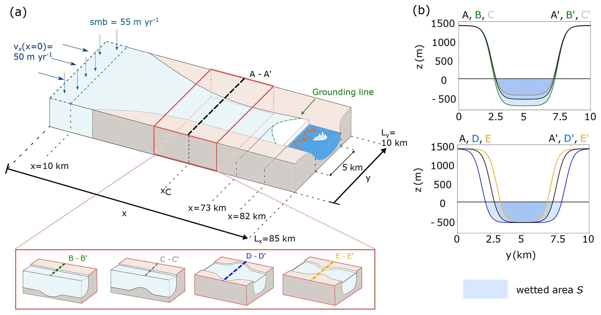
Figure 1 Schematic of the experimental setup. (a) Sketch of the domain (not to scale) with annotated dimensions and mass balance processes (gains: thickness-dependent influx and surface accumulation; losses: melt at the ice–ocean interface and calving). The red box symbolizes how the fjord geometry is changed in different experiments to include geometric perturbations (their center being referred to as x_C). (b) Cross-sections through the linear fjord (black line) and geometric perturbations. Upper panel: basal perturbations (green: depression; gray: bump); lower panel: lateral perturbations (blue: embayment; yellow: bottleneck). The wetted area, i.e., the cross-sectional area of the fjord below sea level, is shaded in blue for each geometry.

2.2 Fjord geometries

Our reference geometry is a fjord sloping linearly towards the ocean with a wide section in the upstream area from which ice is funneled towards a 5 km wide outlet channel with parallel walls (Fig. 1a). The fjord topography is given by $B(x,y)=B_x\left(x\right)+B_y(x,y)$ with

$$\begin{array}{}\text{(4)}& B_x\left(x\right)=B_{\mathrm{0}}+x\times \mathit{\alpha }+\mathrm{\Theta }\left(x\right)\end{array}$$

and

$$\begin{array}{}\text{(5)}& \begin{array}{rl}{B}_y(x,y)& ={\displaystyle \frac{d_{\mathrm{f}}-B_x\left(x\right)}{\mathrm{1}+e^{\left(m_{\mathrm{f}}\left(y-\frac{\mathrm{1}}{\mathrm{2}}{L}_y+w_{\mathrm{f}}+\mathrm{\Omega }\left(x\right)+\mathrm{\Theta }\left(x\right)\right)\right)}}}\\ & +{\displaystyle \frac{d_{\mathrm{f}}-B_x\left(x\right)}{\mathrm{1}+e^{\left(-m_{\mathrm{f}}\left(y-\frac{\mathrm{1}}{\mathrm{2}}{L}_y-w_{\mathrm{f}}-\mathrm{\Omega }\left(x\right)-\mathrm{\Theta }\left(x\right)\right)\right)}}},\end{array}\end{array}$$

where $\mathrm{\Omega }(\mathrm{0}<x<x_{\mathrm{U}})={\frac{x-x_{\mathrm{U}}}{F}}^{\mathrm{2}}$. The parameter values and descriptions are found in Table 1. This formulation is inspired by the Marine Ice Sheet Model Intercomparison Project (MISMIP) setup (Gudmundsson et al., 2012; Asay-Davis et al., 2016) but adapted to our purpose.

To insert basal or lateral perturbations in the outlet channel and thus alter the fjords' depth or width in specific areas, we modify the parameter Θ(x) in either Eq. (4) or Eq. (5) such that

$$\begin{array}{}\text{(6)}& \mathrm{\Theta }(x_B<x<x_E)=-\sin \left({\displaystyle \frac{\mathrm{2}\mathit{\pi }}{\mathrm{\Lambda }}}\left(x-{\displaystyle \frac{\mathrm{\Lambda }}{\mathrm{4}}}-x_{\mathrm{C}}\right)\right){\displaystyle \frac{\mathrm{\Gamma }}{\mathrm{2}}}+{\displaystyle \frac{\mathrm{\Gamma }}{\mathrm{2}}}.\end{array}$$

Altering Θ(x) in only one of the terms on the right-hand side of Eq. (5) allows fjords to be produced with one-sided lateral perturbations, thus making them asymmetric. Combined, these equations reproduce the typical U shape of fjords (Fig. 1b) and yield a setting that is representative of a wide range of outlet glaciers.

Table 1 Parameters for generating fjord geometries (in parentheses for longer geometric perturbations).

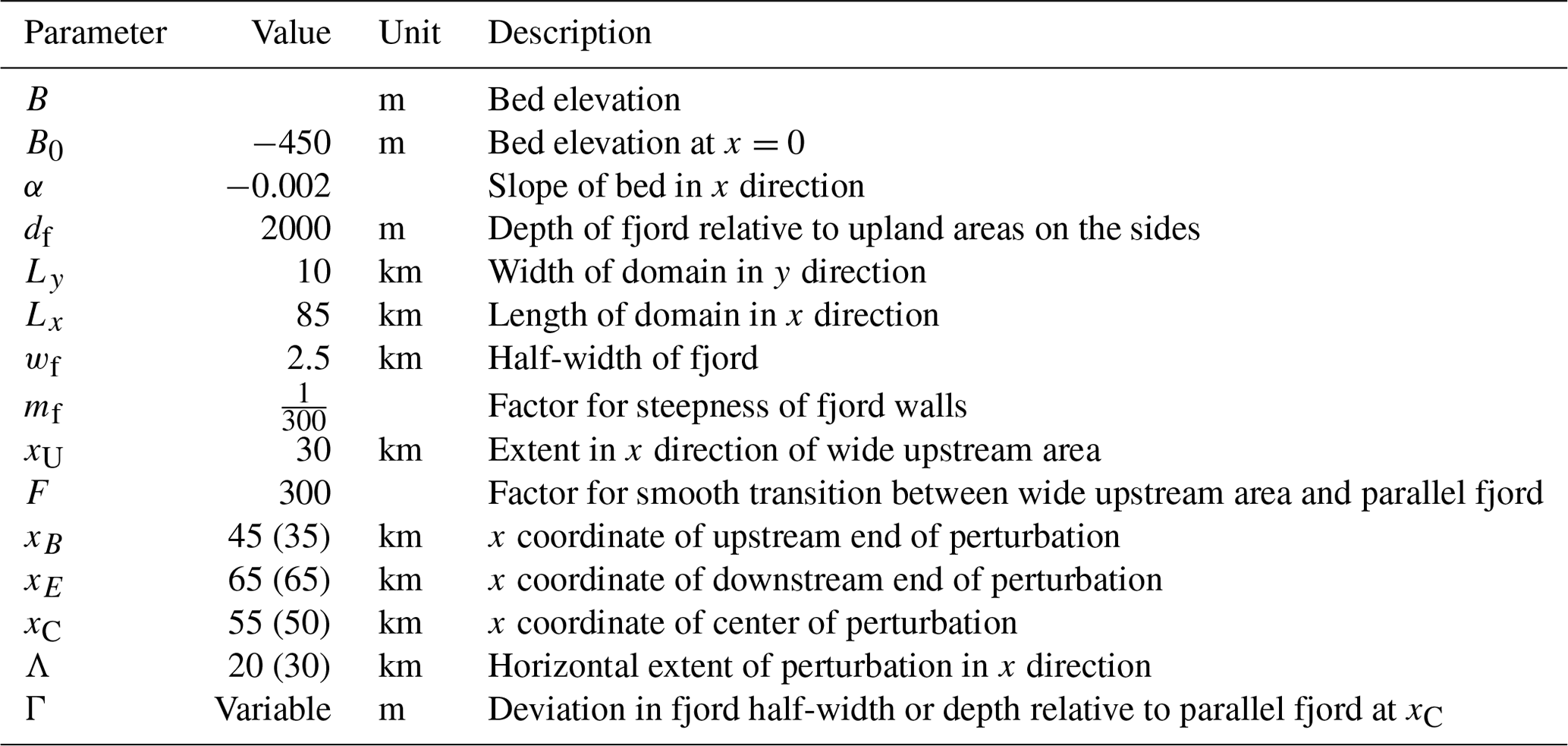
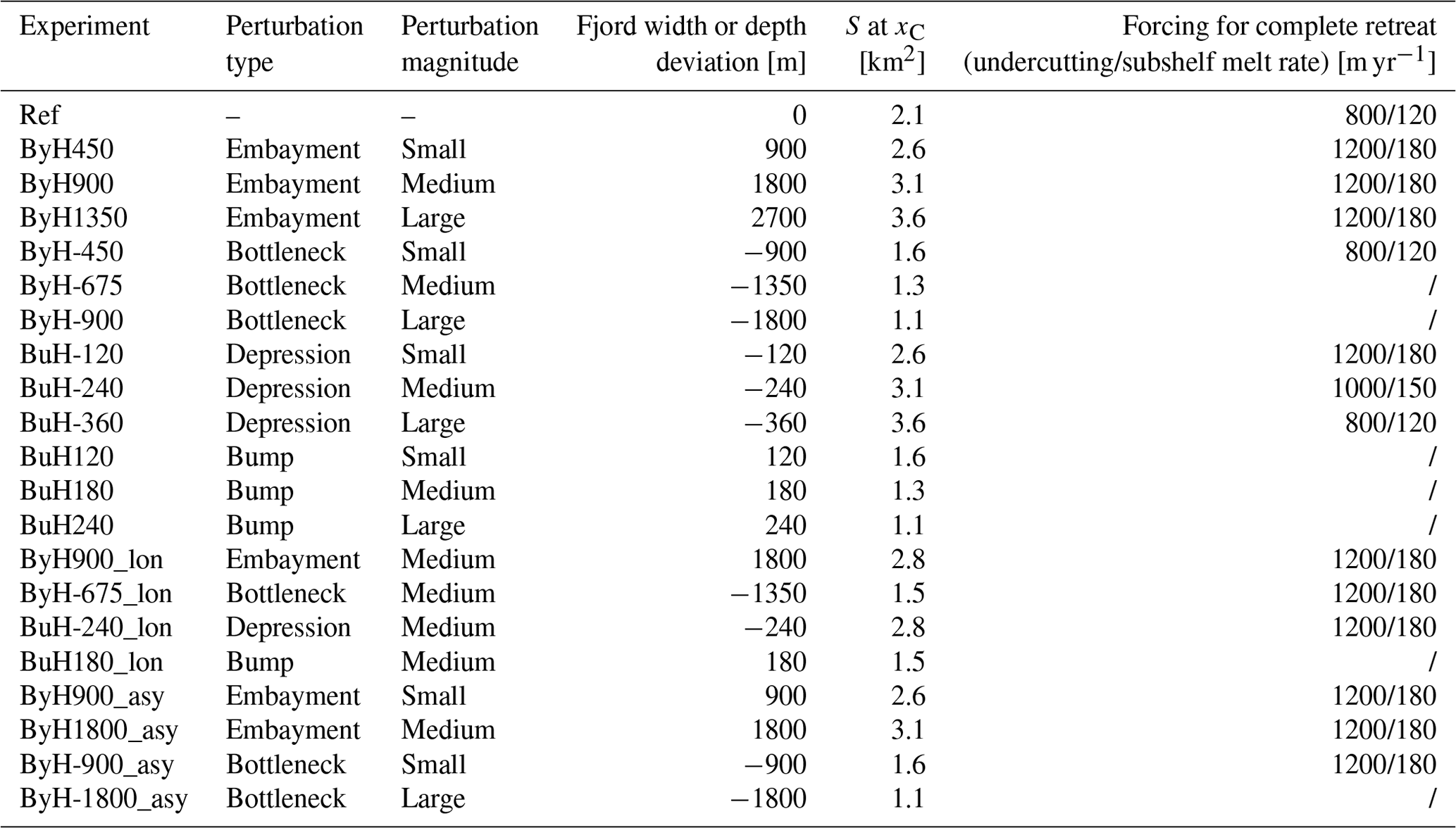
Table 2 Suite of experiments with name (extensions _lon and _asy refer to longer and asymmetric geometries), type of geometric perturbation, perturbation magnitude, the deviation in fjord width (2 Γ for symmetric lateral perturbations, 1 Γ for asymmetric ones) or depth (1 Γ for basal perturbations) at the center of the perturbation relative to the linear reference fjord, S at x_C (i.e., the wetted area at the center of the perturbation), and forcings required to induce complete retreat through the entire geometric perturbation (/ if no complete retreat could be enforced).

The metric used to quantitatively link fjord shape with glacier retreat is the wetted area S: the submerged cross-sectional area of the fjord (Fig. 1b), which can be calculated at any point along an outlet channel according to

$$\begin{array}{}\text{(7)}& S\left(x^{\prime }\right)=\underset{y_{\mathrm{1}}^{\prime }}{\overset{y_{\mathrm{2}}^{\prime }}{\int }}D(x^{\prime },y^{\prime })\mathrm{d}{y}^{\prime },\end{array}$$

where D is the water depth, and $y_{\mathrm{1}}^{\prime }$ and $y_{\mathrm{2}}^{\prime }$ are the intersections of the water line in the fjord with the fjord walls so that $y_{\mathrm{2}}^{\prime }-y_{\mathrm{1}}^{\prime }$ is the width of the outlet channel in a transformed coordinate system that is oriented such that the coordinates $(x^{\prime },y^{\prime })$ are parallel and perpendicular to the center line of the outlet channel, respectively, at any given point. S combines information about the width and depth of a fjord and is thus a comprehensible parameter for comparing basal and lateral perturbations. Furthermore, it is straightforward to calculate its first derivative $\frac{\mathrm{d}S}{\mathrm{d}{x}^{\prime }}$ (in the following written as dS for brevity), which yields information on the along-fjord change in width and/or depth.

Besides our reference setup, we test 20 fjord geometries (Table 2, Fig. 2), each of which contains either a small, medium or large geometric perturbation. The magnitude of the perturbation is defined by how much the width or depth of the fjord deviates from the reference fjord. Our “core experiment”, which the results focus on, comprises 12 fjords, each of which features one of the four perturbation types (depression, bump, bottleneck, embayment) of one of the three magnitude classes (small, medium, large). The depressions and embayments in each magnitude class increase the wetted area S at the center of the perturbation x_C by the same amount, while the bottlenecks and bumps in each magnitude class reduce S at x_C by the same amount. The along-flow horizontal extent of all perturbations in the core experiment is 20 km (Fig. 2).

In the eight simulations outside our core experiments, we test asymmetric and longer perturbations to verify if the results from our core experiment can be transferred to a wider range of settings. We test two asymmetric embayments, which have the same S at x_C as the small and medium embayments and depressions, as well as two asymmetric bottlenecks, which have the same S at x_C as the small and large bottlenecks and bumps. The longer perturbations have an along-flow horizontal extent of 30 km. We test one longer perturbation per perturbation type with S at x_C corresponding to the medium magnitude class.

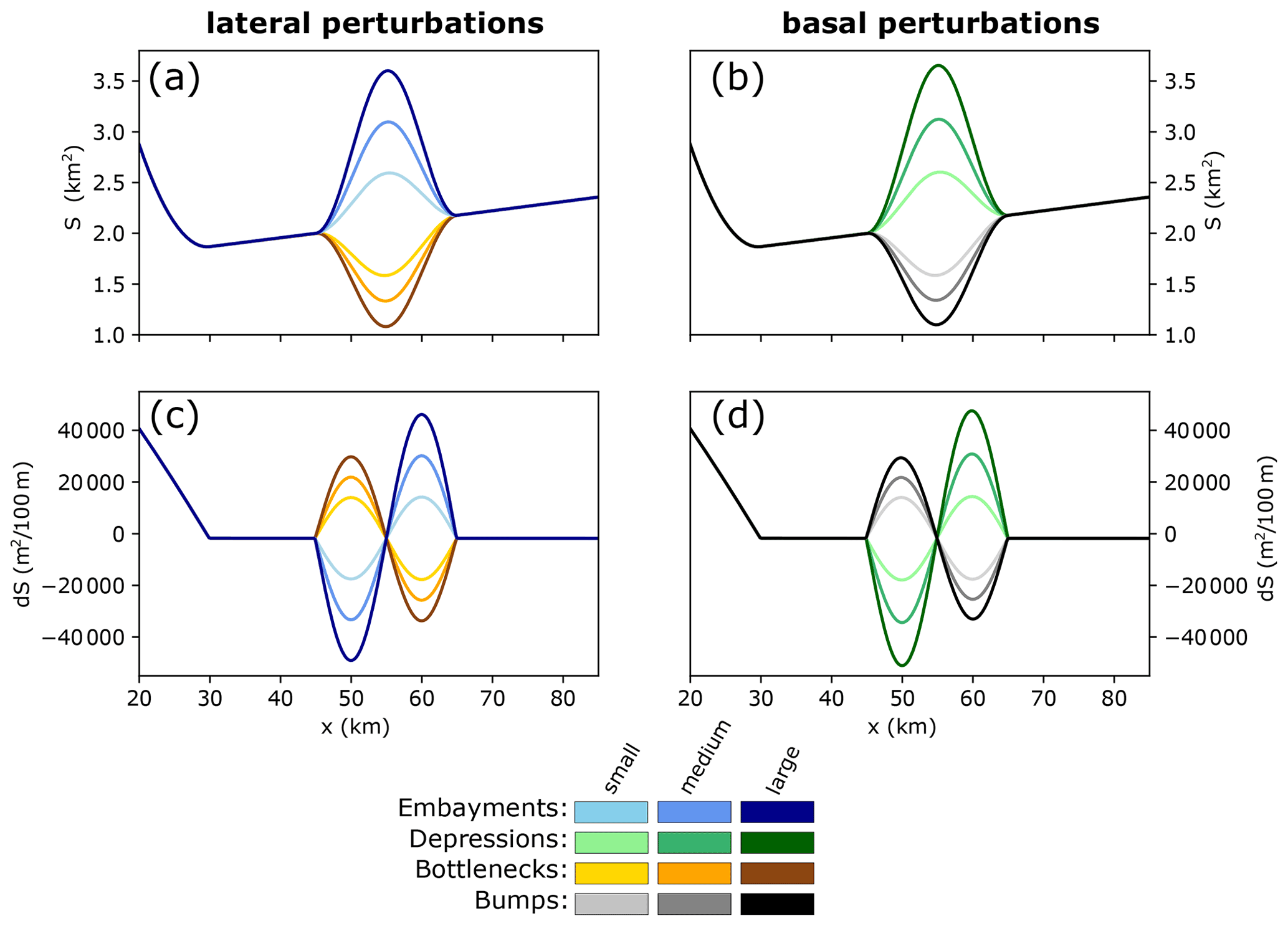
Figure 2 Along-fjord profiles of the wetted area S (a: lateral; b: basal perturbations) and its derivative dS (c: lateral; d: basal) for fjords featuring different geometric perturbations of different magnitude classes. Note that the profiles of embayments and depressions and likewise bottlenecks and bumps of the same magnitude class are largely congruent, thus allowing a straightforward comparison between basal and lateral perturbations.

2.3 Reference glacier

All experiments start from an artificial reference glacier, which is produced by relaxing a rectangular block of ice in the reference fjord. The spin-up is run until the relative ice volume ($(\mathrm{d}V/\text{yr})/V\ll \mathrm{0.05}$ %) and GL position are steady. The length of the spun-up reference glacier is 82 km, its GL is at x=73 km, and the velocity at the GL along the central flow line of the glacier v_GL=2.5 km yr⁻¹. In a steady state, the total mass gain is ∼6.1 km³ yr⁻¹ (≈5.6 Gt yr⁻¹), which is balanced by mass losses through melting at the ice–ocean interface (∼0.9 km³ yr⁻¹) and calving (∼5.2 km³ yr⁻¹). In a sensitivity experiment with doubled ocean melt rates (400 m yr⁻¹ undercutting and 60 m yr⁻¹ subshelf melting), mass loss through ocean melt increases to ∼2.1 km³ yr⁻¹, while calving reduces to ∼4 km³ yr⁻¹. The GL remains largely unchanged, indicating that the reference glacier is not very sensitive to ocean forcing due to compensating effects in the mass wasting processes.

The setup represents a medium-sized fjord–glacier system, which has similar dimensions and dynamics as, for example, the present-day Alison glacier in NW Greenland, where the fjord width is about 5 km, water depth is around 500 m, and observed ice discharge has increased from ∼4 to ∼8 Gt yr⁻¹ in the past 20 yr (Mouginot et al., 2019). It is furthermore broadly representative of outlet glaciers from the Fennoscandian Ice Sheet during the last glacial, such as the Hardangerfjorden glacier (Mangerud et al., 2013; Åkesson et al., 2020).

2.4 Retreat experiments in variable fjords

We slightly modify the reference glacier to match the new fjord geometry when introducing geometric perturbations. For embayments, we extrapolate the glacier surface laterally to fill the newly introduced lateral cavities. For depressions, we fill the new basal cavity with ice but keep the glacier surface the same. For bumps or bottlenecks, we remove ice while keeping the glacier surface unaltered. Subsequently, we relax the glacier in each geometry for 50 yr, resulting in an ice volume change $(\mathrm{d}V/\mathrm{yr})/V<\mathrm{0.5}$ % at the end of relaxation for every setup tested and a steady GL.

After relaxation, we increase the ocean forcing to trigger a retreat. We aim to force the GL to retreat through the entire geometric perturbations. The ocean melt rates required to induce such a retreat depend on the fjord geometry, which we elaborate on in the results section. To determine what melt rates are needed to force this complete retreat in a particular fjord, we strengthen the ocean forcing using multiples of the reference forcing (200 m yr⁻¹ frontal rate of undercutting, 30 m yr⁻¹ subshelf melt) until complete retreat takes place. In some cases (cf. Sect. 3.2), even unrealistically high values for the ocean forcing (e.g., 20 times the reference forcing) did not trigger complete retreat, suggesting that glaciers in these geometries are not sensitive to ocean melt.

Since we want to explore the response of outlet glaciers to melting at the ice–ocean interface, we keep the SMB constant with time and let the upstream ice flux vary only through our parameterized SMB–altitude feedback (Eq. 3).

We assess 16 glacier metrics during the retreat, which we expect to show a response to local topography (Table 3). All of these can be observed in situ or via remote sensing techniques (e.g.,  Mouginot et al., 2019; King et al., 2020), which means that our results are readily transferable to real-world settings. The GL position (x_GL) and its derivative (the GL retreat rate, dGL), the front position (x_Fr) and its derivative (the frontal retreat rate, dFr), and also the velocity at the GL (v_GL) and the shelf length (L_S) are measured along the central flow line of the glacier.

Table 3 Glacier characteristics assessed during retreat for later correlation with fjord geometry. Parameters marked with ^* are assessed along the central flow line of the glacier.

2.5 A real-world case study: Jakobshavn Isbræ

We want to verify the degree to which the dynamics seen in our experiments are also prevalent in real-world settings. This is challenging since we investigate decadal to centennial timescales. Specifically, we would need observations with high temporal resolution on glacier metrics (Table 3) for a glacier that has retreated over tens of kilometers through a fjord with variable and known topography. There are perhaps only a handful of glaciers worldwide that may fulfill these requirements, and even so, acquiring the necessary data is difficult and outside the scope of the present study.

To test our idealized results in a real-world setting, we instead turn to model simulations from the evolution of Jakobshavn Isbræ (JI) in the Holocene (Kajanto et al., 2020). We focus on an 8000-year simulation of the retreat of JI from a sill at the fjord mouth of Jakobshavn Isfjord to a point inland of today's GL position. This model retreat is forced using a step reduction in the equilibrium line altitude early in the Holocene (experiment SE_CM in Kajanto et al., 2020). While this is a sensitivity experiment not meant to reflect the actual evolution of JI (Kajanto et al., 2020), it is convenient for our purposes since it produces a long-lasting, dynamic retreat.

Just like in our idealized experiments, we calculate S and dS for Jakobshavn Isfjord. We then assess whether the relationships found in our idealized settings are also prevalent in JI's dynamics (Sect. 3.5).

3 Results

3.1 Stagnant and ephemeral grounding line positions

We identify positions of GL stagnation (“stagnant” GL positions), i.e., where the GL rests for a sustained time (typically 50 to 200 years) or retreats slowly (dGL $>-$100 m yr⁻¹), and areas where the GL retreats quickly (“ephemeral” GL positions; dGL $<-\mathrm{500}$ m yr⁻¹). Figure 3 shows both stagnant and ephemeral positions for one representative run per perturbation type. For a comparison of the GL retreat dynamics of all simulations within our core experiment, the reader is referred to Fig. A1. Note that in the following, all terminology related to along-fjord changes in width or depth of the fjord (e.g., narrowing, deepening) refers to the direction of glacier retreat.

Stagnant positions exist at the downstream end of embayments and depressions where the fjord becomes wider and deeper (x≈62 to 65 km; Fig. 3a, c). Ephemeral positions, associated with rapid retreat, are found in the remainder of both perturbations (x≈45 to 62 km). Retreat from the stagnant position at the downstream end of the embayment occurs gradually (dGL $\approx -\mathrm{22}$ m yr⁻¹, while x_GL≈62 to 64 km) but is rapidly accelerating as the GL retreats further into the perturbation, accompanied by some lateral ungrounding. Retreat from the stagnant position in the depression occurs suddenly after a phase of near-stability (dGL $\approx -\mathrm{6}$ m yr⁻¹, while x_GL≈64.5 to 65.5 km) as the glacier ungrounds where the fjord is deepest in the center of the perturbation (x≈55 km; Fig. 3c inset plot). The cavity formed under the glacier rapidly grows in size and expands downstream until it eventually detaches the glacier from the bed also at the downstream end of the depression (x≈65 km). In bottlenecks and on bumps, stagnant positions are found where the fjord is narrow and shallow (x≈55 to 58 km; Fig. 3b, d). The stabilizing effect of bumps is, in fact, so large that no glacier could be forced to retreat over them within reasonable limits for the ocean forcing. However, we observe that retreat onto bumps occurs fast (dGL $\approx -\mathrm{500}$ m yr⁻¹ for x_GL≈58 to 65 km). For bottlenecks, only the glacier situated in the fjord with a “small” bottleneck (i.e., the bottleneck with the largest S among the ones tested) could be forced to retreat completely. Noticeably, retreat at the downstream end of the bottleneck (x≈56 to 65 km), where the fjord narrows in, is fast (ephemeral), with dGL $\approx -\mathrm{900}$ m yr⁻¹, whereas it is very slow (relatively stagnant), with dGL $\approx -\mathrm{25}$ m yr⁻¹, upstream of the narrowest point, where the fjord is widening (x≈45 to 55 km; Fig. 3d).

In summary, stagnant GL positions are found where the fjord widens and deepens in the direction of glacier retreat (positive dS; Fig. 2), and rapid retreat occurs through areas where the fjord becomes narrower and shallower (negative dS). Thus, the along-fjord change in width or depth (dS) is a key control on GL retreat. However, glaciers in narrower or shallower fjords than the reference fjord (bottlenecks and bumps) can also temporarily stagnate where S is small. This shows that the wetted area constitutes an additional important control on GL retreat. The experiments with asymmetric and longer perturbations confirm these findings (see Fig. A2).

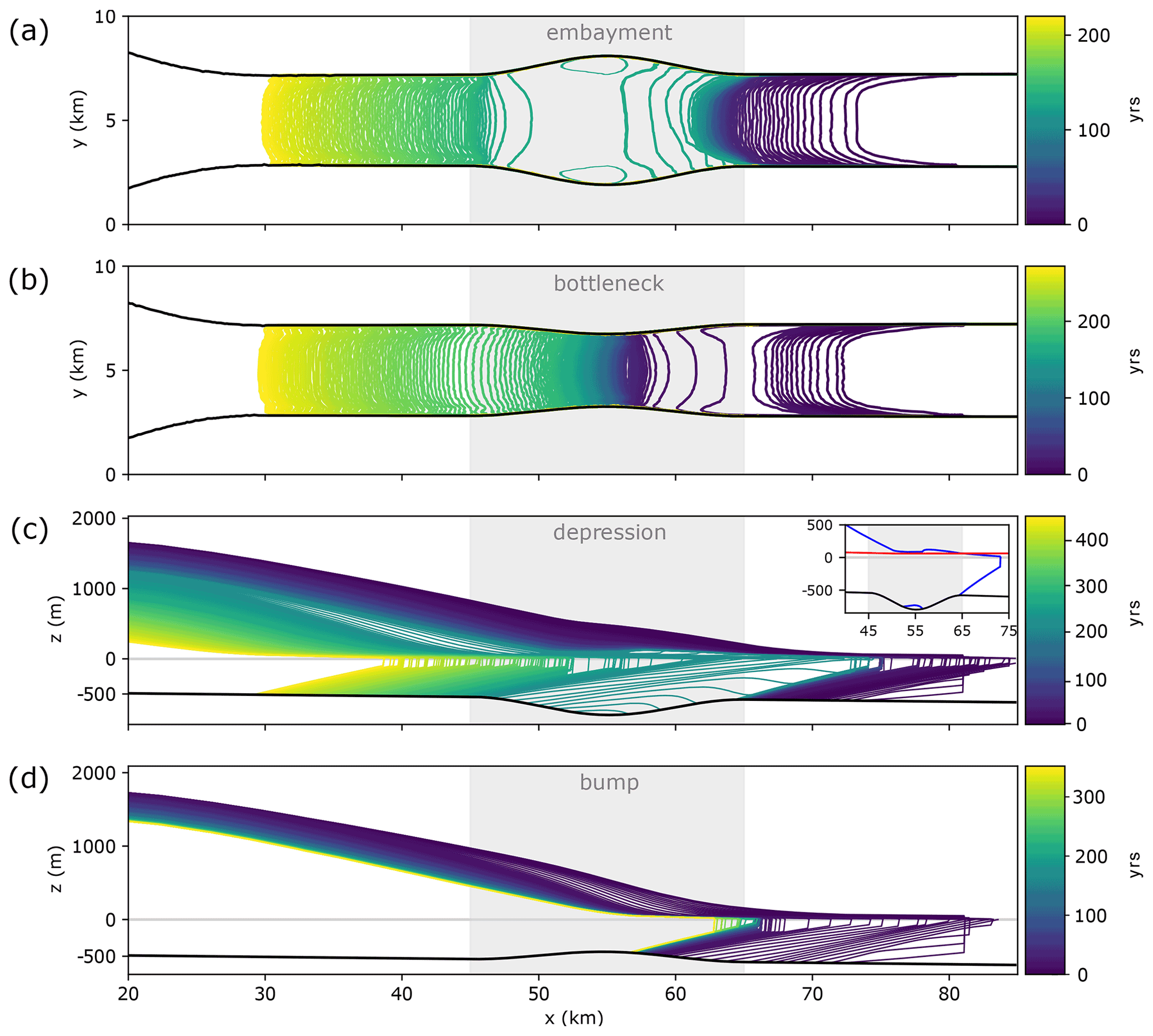
Figure 3 Annual glacier evolution (a, b: top-down view of domain showing yearly grounding lines; c, d: yearly glacier profiles along central flow line) in fjords featuring different geometric perturbations (location of perturbations marked in gray) with the spacing between the lines indicating retreat velocity: (a) medium embayment, (b) small bottleneck, (c) medium depression, (d) small bump. Inset plot in (c) shows profile (blue) in year 217 when glacier ungrounds in the central part of the depression, which triggers further retreat. The red line is the level to which a glacier needs to thin to reach flotation.

3.2 Forcings and timings of retreat

Now, we investigate how retreat from stagnant and ephemeral GL positions is correlated with fjord topography (i.e., S and dS). Two parameters are important in this context (Fig. 4): first, the amplitude of the forcings needed to induce complete retreat through the different geometric perturbations. As mentioned previously, distinctions exist between both the different perturbation types (bumps, depressions, bottlenecks, embayments) and the different magnitude classes (small, medium, large) for a given geometry type. The second important parameter is the approximate residence time of the GL in a stagnant position. The stronger the GL is stabilized by a particular geometric perturbation, the longer it will be stagnating.

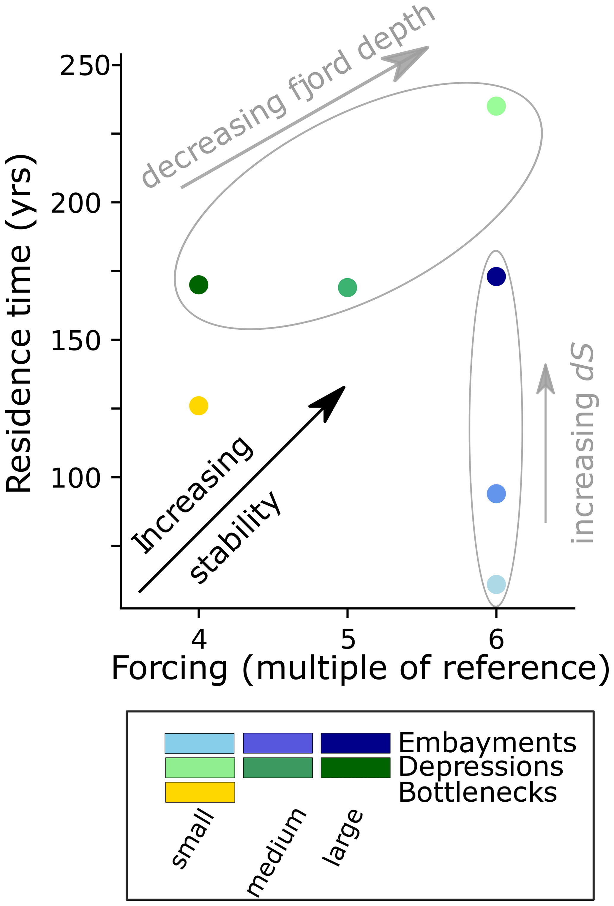
Figure 4 Forcing required to induce complete retreat in multiples of the reference forcing (200 m yr⁻¹ undercutting rate, 30 m yr⁻¹ subshelf melt) and approximate residence time of the GL in a stagnant position for different fjord geometries. A longer residence time and a larger forcing required indicate that fjord geometry provides larger stability. More stability is correlated with decreasing fjord depth for depressions (shades of green) and with increasing along-fjord change in wetted area dS for embayments (shades of blue). The simulations for which no retreat through the perturbation was observed have been omitted from the figure.

All glaciers in embayments require the same increase in forcing to retreat completely (6 times the spin-up forcing). This increase is larger than what is needed to induce retreat through the linear reference fjord (4 times the spin-up forcing). The residence time of the GL in the stagnant positions at the downstream end of the embayments is such that the glacier in the smallest embayment is the earliest to retreat (after 61 yr of GL stagnation), and the one in the largest is the latest (after 173 yr) (Fig. 4). This implies that the larger the embayment, the more stability it provides to the glacier at its downstream end before retreat through the entire perturbation is possible. A larger embayment means a locally larger along-flow change in wetted area dS at its downstream end (Fig. 2). Thus, there is a positive correlation between GL stability and dS. This indicates that dS not only determines the location of stagnant GL positions in embayments, as shown before, but that it also quantitatively impacts how stagnant the GL is.

The glaciers in fjords with depressions require different forcings to retreat completely (small: 6× the reference forcing; medium: 5×; large: 4×). The residence time also varies; retreat over small depressions occurs ∼65 yr later than over medium and large depressions, which retreat after about the same time (after 169 and 170 yr, respectively). These findings indicate that the stabilizing effect of a depression declines the deeper it is (Fig. 4). Thus, there is a negative correlation between GL stagnation and S. In Sect. 3.1, ungrounding in the central part of depressions was identified as the trigger of rapid retreat from the temporary stillstands. Such GL retreat occurs more easily in a deeper fjord (larger S). Therefore, it is consequential that a deeper depression is less stabilizing. Note, however, that the fjord depth several kilometers upstream of the GL determines how long the GL stagnates. There is no direct correlation between S or dS at the GL and the stability provided to the glacier by the fjord in our settings with depressions.

The glacier in a fjord with a “small” bottleneck required a 4-fold increase in oceanic melt rates and retreated from its stagnant position after 126 yr of stagnation. This is a weaker forcing than for the glaciers in the embayments as well as for the medium and small depressions and thus suggests that this bottleneck provides less stability than these geometries. This contrasts with the common pattern, where a small S and a positive dS should stabilize the glacier strongly. It is unclear why this is the case here. We hypothesize that it might be related to a combination of high driving stresses due to a steepened surface inside the bottleneck in conjunction with high modeled calving rates (not shown). The two experiments with glaciers in geometries with narrower bottlenecks (“medium” and “large” bottleneck) did not retreat through the entire perturbation. This, in turn, aligns well with the general notion of a confined (low S) and downstream narrowing (positive dS) fjord yielding strong stability to the glacier. Likewise, none of the glaciers in fjords with bumps retreated completely, which follows the same concept. However, the strong stability that bumps provide to the glacier may also be related to the choice of model parameters (Sect. 4.2).

3.3 Stress balance response to fjord geometry

To assess the underlying mechanisms behind the geometric controls described before, we now analyze the stress regimes across the studied geometries. We focus on lateral shear stress gradients for lateral perturbations and longitudinal stress gradients for basal perturbations as given by the SSA in the x direction by

$$\begin{array}{}\text{(8)}& \mathit{\rho }gH{\mathit{\alpha }}_x={{\mathit{\tau }}_{\mathrm{b}}}_x+{\displaystyle \frac{\partial }{\partial x}}(\mathrm{2}H{\mathit{\sigma }}_{xx}^{\prime }+H{\mathit{\sigma }}_{yy}^{\prime })+{\displaystyle \frac{\partial }{\partial y}}\left(H{\mathit{\sigma }}_{xy}^{\prime }\right),\end{array}$$

where σ^′ is the deviatoric stress, and τ_b is basal drag. We interpret the second and third term on the right-hand side as longitudinal stress gradient and lateral shear stress gradient, respectively. With the imposed spatially uniform friction coefficient, variations in the investigated stress fields are largely caused by variable fjord topography and are hence convenient to investigate for our purpose.

For embayments and bottlenecks, variations in lateral shear stress gradients can be seen along the fjord walls (Fig. 5a, b). Specifically, strongly negative shear stresses are found where ice is funneled in a downstream narrowing fjord. This occurs, for example, where 55 km $<x<$65 km in embayments (Fig. 5a) and where 45 km $<x<$55 km in bottlenecks (Fig. 5b). This indicates enhanced resistance to flow for the glacier originating from the fjord walls, which provides stability to the glacier. Where ice flow diverges in a widening section of the fjord (in the upstream half of embayments and the downstream half of bottlenecks; Fig. 5a, b), lateral shear stress gradients are comparatively weak. This indicates that the glacier–fjord wall contact is reduced here and that the fjord walls provide little support to the glacier in these areas.

For depressions and bumps, we see clear variations in longitudinal stress gradients along the glacier bed (Fig. 5c, d). In depressions, a band of negative values stretches across the full width of the outlet channel where the bed turns from being prograde to retrograde (at x=55 km; Fig. 5c), indicating that ice flow is being blocked here. Likewise, a marked reduction in positive longitudinal stresses is seen at the onset of the bump where the bed slope switches sign (at x=45 km; Fig. 5d). Together, the stress regimes in basal perturbations demonstrate that a retrograde glacier bed, tilted against the direction of flow, reduces longitudinal stress gradients considerably as it increases the basal resistance to flow, which ultimately stabilizes the glacier.

In summary, the stress analysis above suggests that increased lateral shear stress gradients or negative longitudinal stress gradients are found wherever ice flow is forced to converge, either horizontally or vertically, towards a narrowing or shoaling area downstream. Simulations using asymmetric as well as longer perturbations confirm that these findings are robust (see Fig. A3). Through the convergent flow, the contact between the glacier and the fjord is enhanced, leading to increased resistance to flow. Overall, along-flow change in fjord width or depth (i.e., dS) is found to define areas of increased lateral shear gradients or negative longitudinal stress gradients and thus GL stagnation.

Figure 5 Stress states in perturbations. Lateral shear stress gradients for (a) and (b), with flow lines in gray, and longitudinal stress gradients for basal perturbations (c, d). The green line is the grounding line; the black line is the glacier outline.

3.4 A quantitative relationship for ice–topography interaction

We hypothesize that there is a quantitative relationship between fjord geometry and glacier retreat, valid across a range of different geometries. To test this, we correlate a variety of metrics indicative of glacier retreat (Table 3) against relevant metrics of fjord geometry, that is, the submerged cross-sectional area (S) and its derivative (dS). We restrict the data to those instances when the GL is located within a geometric perturbation (gray-shaded areas in Fig. 3). Among all combinations of retreat and geometry metrics tested, including those of asymmetric and “longer” perturbations (Table 2), the clearest and most universal relationship found is a negative, close-to-linear correlation between the ratio of the GL flux and the submerged cross-sectional area $Q_{\mathrm{GL}}/S$ over the change in submerged cross-sectional area dS (Fig. 6). This relation expresses that a widening or deepening fjord in the downstream direction (negative dS) promotes a high GL flux per wetted area ($Q_{\mathrm{GL}}/S$). Conversely, a glacier retreating in a fjord that becomes narrower or shallower downstream (positive dS) will have a reduced $Q_{\mathrm{GL}}/S$. Note that the ratio $Q_{\mathrm{GL}}/S$ for basal geometry perturbations (gray to black and green colors in Fig. 6) is on average lower than for lateral geometry perturbations. This means that basal perturbations generally inhibit ice flux across the GL more efficiently than lateral perturbations (note that this may be influenced by our modeling choices; Sect. 4.2). Also, note that the GL flux is the product of the velocity v_GL and the flux gate area at the GL A_GL, that is $Q_{\mathrm{GL}}=v_{\mathrm{GL}}\times A_{\mathrm{GL}}$. The ratio $Q_{\mathrm{GL}}/S$ is thus proportional to v_GL when there is hydrostatic equilibrium at the GL (because in that case, $S=\mathrm{0.9}\times A_{\mathrm{GL}}$), and so we find a comparable, negative linear relationship between v_GL and dS (Fig. A4).

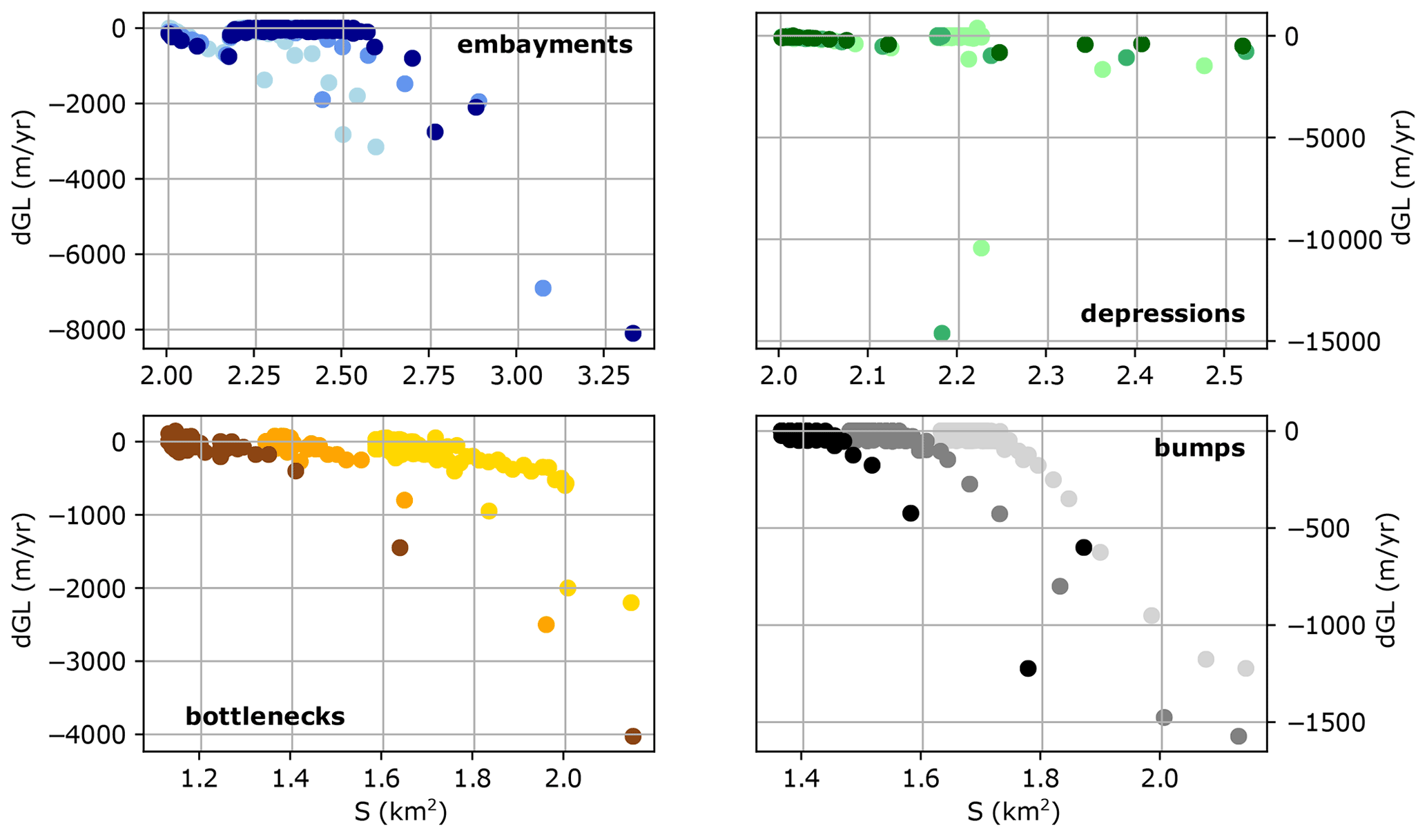
We find an additional yet less distinct negative relationship between the wetted area S and the GL retreat rate dGL (Fig. 7a). This shows that a wider or deeper fjord promotes faster GL retreat, while a narrower or shallower geometry stabilizes the glacier. This relation is not as universal as the previous one since one value for dGL is not uniquely linked to one value for S across different geometries. Furthermore, it is not linear but rather such that for a range of low S values, dGL does not vary noticeably. Only above a certain threshold in S does the GL retreat markedly faster (Fig. 7b). This threshold varies between different fjord geometries. However, we find that it is always associated with the location of GL stagnation (Fig. 3.1). This means that a relationship between GL retreat rate dGL and S only unfolds if a local stability position is passed. These stagnant positions can be either where S is low or where dS is high, as shown previously. For instance, dGL does not increase as the GL retreats very slowly at the stagnant position in the downstream half of embayments. Only once it has retreated passed this point of GL stagnation can a correlation between dGL and S be seen.

For depressions we do not see a distinct relationship between dGL and S (Fig. SA5). This is because we measure the GL position x_GL and therefore also dGL as the farthest downstream grounded point along the central flow line of the glacier. When the glacier ungrounds in the center of a depression, where the fjord is deepest, the dynamics of retreat are triggered several kilometers upstream of the GL, as mentioned in Sect. 3.1. Therefore, there is a correlation between fjord depth and GL retreat in depressions. However, it is not reflected when only considering processes at the GL. Not finding a dGL-over-S relation for depressions is hence expected by construction of our methodology and not an actual feature.

Figure 6 Relationship between grounding line discharge per wetted area $Q_{\mathrm{GL}}/S$ and along-fjord change in wetted area dS for all tested geometries and all instances when the GL is within a geometric perturbation (gray area in Fig. 3).

Figure 7 Relationship between grounding line retreat rate dGL and wetted area S. (a) All instances when the grounding line is within a geometric perturbation for all tested geometries, except for depressions since retreat in these perturbations is governed by different dynamics than in the ones shown. (b) Schematic of a typical relationship between dGL and S, where dGL is constant for low S, while high S induces faster retreat. The transition between these two states occurs if the GL retreats past a point of GL stagnation. The location of these points may be controlled by either low S or high dS.

3.5 Jakobshavn Isbræ

Given our previous results, we now aim to assess whether our principal geometric relationship $Q_{\mathrm{GL}}/S$ over dS can be found for Jakobshavn Isbræ. To this end, we calculate the wetted area S along the topography of Jakobshavn Isfjord as used in Kajanto et al. (2020), which depicts overall higher values and larger along-fjord changes in dS than our idealized settings (Fig. 8b).

Plotting all available data points for $Q_{\mathrm{GL}}/S$ over dS at Jakobshavn, we do not find the aforementioned geometric relationship. This may have many reasons related to the complex dynamics of Jakobshavn Isbræ (Bondzio et al., 2017), but most critically, there is lateral inflow of ice to the main channel from the surrounding ice sheet and tributaries (compare with Steiger et al., 2018). This alters the stress balance at the GL compared to our experiments, where the glacier is always closely confined between fjord walls. Specifically, it means that the rigid glacier–wall interface in our experiments is replaced by a changing ice–ice contact. This has implications for the lateral friction that the fast-flowing ice in the main channel experiences and for the processes transferring stabilizing back stress from the sides to the center of flow.

We thus expect our findings to be more easily transferable to settings where Jakobshavn Isbræ is enclosed by fjord walls. This is only the case in one part of the outlet channel, upstream of the present-day front (Fig. 8c). Indeed, values for $Q_{\mathrm{GL}}/S$ are inversely related to dS in a qualitative way here such that an increase in dS is generally associated with a decrease in $Q_{\mathrm{GL}}/S$ and vice versa (Fig. 8d, e), consistent with our findings for synthetic geometries above (Fig. 6). Even though this relationship is only qualitative, meaning that one value for dS is not uniquely associated with one value for $Q_{\mathrm{GL}}/S$, we find these results encouraging given the complexity of Jakobshavn Isbræ's dynamics. For settings resembling our setup more closely, such as medium-sized outlet glaciers found in, for example,  Greenland (Carr et al., 2014; Bunce et al., 2018; Catania et al., 2018), Svalbard (Schuler et al., 2020) and Novaya Zemlya (Hill et al., 2017), we expect an even stronger imprint of topography on retreat dynamics.

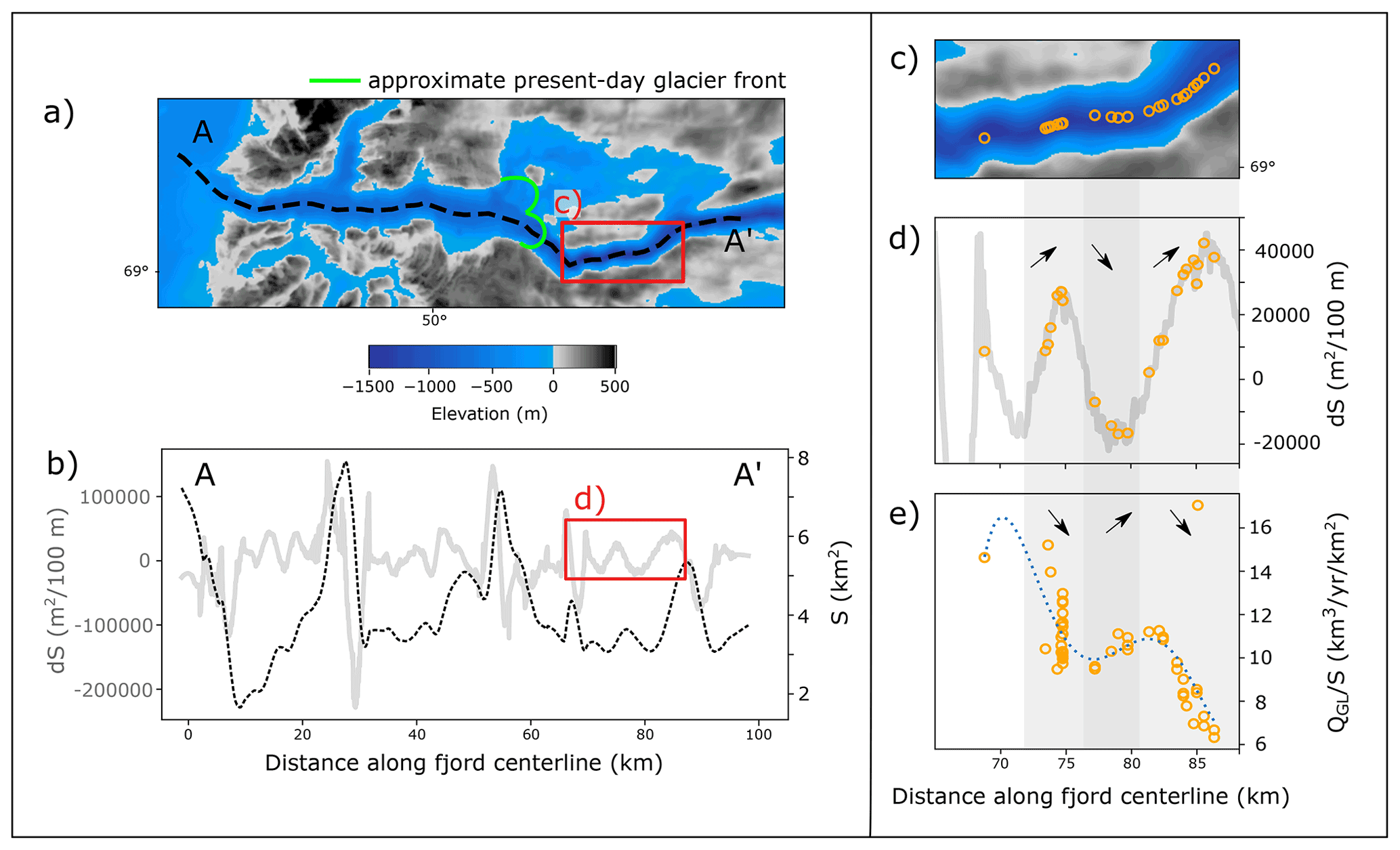
Figure 8 The real-world example Jakobshavn Isbræ. (a) Topography of Jakobshavn Isfjord (Morlighem et al., 2017) with approximate present-day glacier front and centerline along which profiles shown in (b) of the wetted area S and its along-fjord change dS are calculated; (c) zoom to area where JI is enclosed between fjord walls, with yellow circles showing all modeled grounding line positions in this section (Kajanto et al., 2020); (d) dS profile in the same section of the fjord with grounding line positions indicated; (e) $Q_{\mathrm{GL}}/S$ in this section with grounding line positions and a polynomial fit (dotted blue line). The opposing trends in dS (d) and $Q_{\mathrm{GL}}/S$ (e) as indicated by the arrows demonstrate qualitatively that the negative relationship $Q_{\mathrm{GL}}/S$ over dS can be found in this complex setting.

4 Discussion

4.1 Mechanisms behind geometric controls of glacier dynamics

The current study offers new quantitative insights into how topography influences the evolution of marine outlet glaciers and their response to ocean warming. We demonstrate that two topographic metrics, the wetted area S and its derivative dS, jointly control the dynamics and retreat of glaciers constrained by fjord walls. Together, these metrics largely explain variations in grounding line mass flux Q_GL, which is important in the context of sea-level rise, and the grounding line retreat rate dGL.

Based on our stress analysis and physical principles, we propose the following physical interpretation for these results: first, a downstream narrowing or shoaling fjord (positive dS) stabilizes the glacier as ice flow is funneled through the constriction enhancing the glacier–fjord contact (Fig. 5a, c). This increases the basal or lateral resistance to flow, which stabilizes the glacier. Conversely, a downstream widening and deepening fjord (negative dS) provides little support to the glacier as glacier–fjord contact is reduced (Fig. 5b, d). Second, a narrow fjord (low S) stabilizes the glacier because the distance between the lateral ice margins, where friction with the fjord walls is high, and the center of flow is small. This means that the part of the glacier where ice flow is largely undisturbed is reduced (Raymond, 1996; van der Veen, 2013). Third, a shallow fjord (low S) stabilizes the glacier because the glacier is further away from flotation, and thus grounding line retreat is less likely to occur with a given amount of thinning (Pfeffer, 2007; Enderlin et al., 2013). In our experiments, the area exposed to ocean melt does not have a large effect on retreat dynamics. Even high oceanic melt rates, which could compensate for a small ice–ocean interface, do not trigger retreat through geometric perturbations where S is low.

For a particular fjord geometry, the relative importance of S or dS in providing stability to the glacier may vary. This is discussed with two examples from our results: in embayments, S is larger than the reference fjord. Therefore, if S was the dominant control for glacier dynamics here, retreat through embayments should occur more easily than through the reference fjord. However, we find that the opposite is true; the grounding line stagnates at the downstream end of embayments (Fig. 3a), while it retreats steadily through the reference fjord (Fig. A1). This indeed confirms that S alone does not explain glacier retreat. Rather, dS controls glacier dynamics because the point of grounding line stagnation is where the fjord changes from wide to narrow in the direction of ice flow. For bed bumps in our experiments, the picture is different. Our model glaciers stagnate on or near the crest of the bumps, where dS is close to 0 or negative (Fig. 3d). This should not be an obstacle for retreat if dS was the dominant control on glacier dynamics. Therefore, it must be the shallowness of the fjord at this point (indicated by low S) which governs the dynamics here.

Given these disparities between different settings, it is all the more compelling that we find the geometric relationship $Q_{\mathrm{GL}}/S$ over dS universal to all our idealized fjords. It implies that given the current grounding line mass flux Q_GL and the upstream subglacial topography of a particular glacier, a well-founded estimate of the topographically induced future contribution to sea-level rise can be made. To the authors' knowledge, this type of quantitative link between fjord topography and glacier response has not been established before, going beyond the qualitative descriptions of ice–topography interaction offered in previous studies (Enderlin et al., 2013; Carr et al., 2014; Bunce et al., 2018; Catania et al., 2018; Åkesson et al., 2018b). For projections of future sea-level rise, this direct coupling between topography and ice discharge is highly relevant as it enables an ad hoc assessment of the expected future sea-level contribution of a glacier on decadal to centennial timescales. Q_GL is readily available for glaciers where the velocity and bathymetry are well known. However, the physical interpretation of the relationship between $Q_{\mathrm{GL}}/S$ and dS is not straightforward. Since $Q_{\mathrm{GL}}/S$ is proportional to v_GL when there is hydrostatic equilibrium at the grounding line, the expression can be thought of as relating grounding line velocities to along-fjord changes in fjord topography through the mechanisms described in our stress analysis (Sect. 3.3). Accordingly, our results show that velocity evolution at the grounding line over time is also a good proxy for the dynamic response of a glacier to fjord topography (Fig. A4). This may be specifically useful for less well-studied glaciers with unknown bathymetry. Notably, our geometric relationship is distinct from a typical mass-conservation argument, which simply states that velocities must increase for a decreased flux gate, and vice versa, to maintain the same grounding line discharge. This is because in such an argument, velocities are related to absolute values of fjord width or depth and not the along-fjord change in fjord geometry. While mass-conservation mechanisms certainly play a role in our simulations, we do not find that such a relationship alone is sufficient to fully explain the dynamics we observe.

Our second quantitative relationship between dGL and S confirms the widely accepted concept that a wide or deep fjord promotes fast grounding line retreat (e.g., Warren and Glasser, 1992; Enderlin et al., 2013; Carr et al., 2013; Bunce et al., 2018; Catania et al., 2018; Åkesson et al., 2018b). However, we highlight that this relationship may not hold if the fjord is narrowing or shoaling downstream (positive dS). In practical terms, this means that retreat from a uniformly wide and deep channel into an upstream-widening or upstream-deepening section does not automatically imply that retreat has to accelerate. Rather, we suggest that a glacier will sit at the downstream end of the section, where S is increasing upstream, for a considerable time or may not even retreat further because it is particularly stagnant here. Only if this position is abandoned will fast retreat occur (Fig. 5a). This fast retreat is in fact facilitated by the long residence time of the grounding line since concurrent upstream-thinning preconditions the glacier for fast retreat.

In contrast to most previous studies, we emphasize the role of along-fjord change in fjord topography (dS) to explain geometric controls of outlet glaciers. Along-fjord change in fjord depth is also key in the context of the marine ice sheet instability (MISI) theory, according to which retrograde beds promote retreat (Schoof, 2007; Gudmundsson et al., 2012; Gudmundsson, 2013). However, even though we do have retrograde beds in our fjords with basal perturbations, we do not see any influence of the MISI on glacier dynamics. This is simply because our tested glaciers never retreat into an area where the bed slope is strongly negative and where the MISI effect would be expected to occur. On bumps, the glaciers stop to retreat on the downstream side, where the bed is prograde (Fig. 3d). In depressions, the grounding line stagnates where the bed slope is only slightly negative (Fig. 3c), which is not enough to trigger a MISI feedback loop. Retreat off this stagnant position occurs through ungrounding several kilometers upstream of the grounding line. This process is not related to typical MISI dynamics. Besides that, our quantitative relation $Q_{\mathrm{GL}}/S$ over dS may seem contradictory to widely accepted concepts of glacier dynamics because we project high $Q_{\mathrm{GL}}/S$ for prograde beds (i.e., negative dS in our study). This may give the impression that prograde beds should lead to accelerating ice discharge. However, we emphasize that we assess ice discharge per area, not absolute values of ice discharge. A glacier retreating on a prograde bed will experience a reducing wetted area as it recedes, and thus the ratio $Q_{\mathrm{GL}}/S$ may increase but not the absolute grounding line flux. This is exemplified by our experiments with bumps, where the glacier stagnates on a prograde bed even though $Q_{\mathrm{GL}}/S$ is relatively high (Fig. 6).

Only a few studies have considered the influence of along-fjord changes rather than absolute values in fjord width on glacier dynamics, and available observations are limited in time (Carr et al., 2014; Bunce et al., 2018). The main consensus is that a fjord widening in the direction of glacier retreat promotes fast grounding line recession, while a narrowing fjord reduces retreat rates. Furthermore, retreat onto a pinning point can stabilize the grounding line. This is related to our findings in that we also see accelerating retreat the further the grounding line moves into a wider fjord upstream (cf. grounding line positions in the downstream half of the embayment (55 km $<x<$ 65 km) in Fig. 3a). However, in our results, this only occurs after a phase of grounding line stagnation at the downstream end of such fjord sections. We do not find conclusive evidence in the observational record whether these points of grounding line stagnation are a relevant phenomenon in real-world settings or not (Carr et al., 2014; Bunce et al., 2018; Catania et al., 2018). Further research analyzing a range of fjord geometries and glacier retreat histories is required to test this result. We do see some signs in our experiments that retreat slows down the further the grounding line recedes into a narrower fjord upstream. Overall though, retreat in upstream-narrowing fjords is markedly faster than if the fjord is upstream-widening (compare grounding line positions in the downstream half of bottlenecks (55 km $<x<$ 65 km) with the ones in the upstream half (45 km $<x<$ 55 km) in Fig. 3b). This we explain with the aforementioned enhancement (reduction) in fjord–glacier contact for an upstream-widening (upstream-narrowing) fjord (Fig. 5a, b). Thus, we confirm that retreat slows down in an upstream-narrowing fjord, but in the context of a retreat cycle through both upstream-widening and upstream-narrowing fjord sections, overall faster retreat occurs through upstream-narrowing fjords. Therefore, the observational records of glacier retreat in Greenland may be too short and the fjord-width variations too small to attest to similar dynamics as we observe in the model (Carr et al., 2014; Bunce et al., 2018; Catania et al., 2018). However, in line with the observational record, we can reproduce the stability that lateral pinning points offer. This is clearly demonstrated by the strong stability that narrow bottlenecks provide in our experiments.

Our experiments are set up to simulate grounding line retreat, and hence we do not offer any insights on ice–topography interactions for advancing glaciers. Previous studies, however, suggest that fjord geometry induces hysteresis in the retreat–advance cycle of a glacier, meaning that a reversal to colder conditions after a phase of climate warming does not allow the grounding line to advance to the same position it occupied initially if the fjord is widening or deepening in front of the glacier (Brinkerhoff et al., 2017; Åkesson et al., 2018b). We expect this also to hold for our experiments if we had simulated ocean cooling following the warming scenarios tested.

4.2 Study limitations

As in all numerical studies, our results have limitations related to the choice of model parameters. In particular, there are three aspects that warrant further discussion. First, the SSA used here is not a full representation of the stress regime in a glacier, which especially bears relevance near the grounding line. For weak beds and fast-flowing outlet glaciers, as we aim to mimic in our synthetic setup, the SSA is a reasonable approximation and widely used in the glaciological literature. It may fail, however, on steep bed slopes, such as the ones in our simulations of basal perturbations. In particular, the effect of basal high-friction points may be overestimated, which might explain why basal perturbations generally yield lower $Q_{\mathrm{GL}}/S$ values than lateral perturbations in our experiments (Fig. 6) and why bumps were found to be excessively stabilizing. However, we do not expect this effect to compromise our conclusions in general. For instance, Favier et al. (2012), using a setup similar to ours to simulate the effect of a basal pinning point on ice dynamics with a full-Stokes model, present stress distribution patterns that agree favorably with the ones shown here. The influence of using the SSA as compared to a full-Stokes model on our results is therefore expected to be limited.

Second, choosing a Budd-type friction law which introduces an elevation dependence of the basal friction through the effective pressure adds complexity to the interpretation of our results. Specifically, it means that bed bumps and depressions alter the basal resistance to flow purely through their elevation difference to the surroundings. This may be another reason why no retreat over bumps was possible in our experiments. Furthermore, while the Budd friction law is one of the most commonly used ones, previous studies have also shown that different friction laws can lead to substantial differences in transient ice dynamics and steady states (Brondex et al., 2017; Åkesson et al., 2021). A comparison between different friction laws is outside the scope of this study, and thus the impact of this modeling choice is difficult to estimate. Third, the calving parameterization chosen is an important control on the simulated dynamics. Other idealized studies have applied a calving law with a prescribed ice front position or a prescribed ice shelf length (Schoof et al., 2017; Haseloff and Sergienko, 2018), which both have the disadvantage of being unknown in general, whereas we opt for the von Mises parameterization due to its relatively good performance when applied to real-world glaciers (Choi et al., 2018). Again, in the absence of a universal calving law, the potential effect of this modeling choice on our results is hard to assess. Overall, it can be assumed that the geometric relationship found here is not as distinct in complex real-world settings. The degree to which our results are transferable to a specific glacier will depend on the degree to which the stress regime at the glacier front and the grounding line is comparable to our setup. This is what we demonstrated with the example of Jakobshavn Isbræ. Nonetheless, since we use a state-of-the-art model with parameterizations that have been calibrated against typical values for marine outlet glaciers, we expect our findings to be applicable to a wide range of settings.

Many of the medium-sized glacier catchments in Greenland may yield a long-term contribution to sea-level rise as thinning at the outlet glaciers may propagate far upstream (Felikson et al., 2021). Here, we offer a quantitative perspective on the processes at the grounding line and highlight the importance of assessing both the wetted area and the along-fjord change in wetted area in order to accurately describe ice–topography interactions. These two parameters together determine the geometrically induced ice discharge to the ocean, which is crucial for sea-level rise, and the expected future retreat of marine outlet glaciers.

5 Conclusions

The shape of a fjord can promote or inhibit glacier retreat in response to climate change. Here, we use a numerical model to study such ice–topography interactions in a synthetic setup under idealized conditions. We find that variable fjord topography induces gradients in lateral or basal shear stresses, which then influence glacier dynamics. Increased shear at the ice–fjord interface, which stabilizes the model grounding line, is caused by converging flow towards a downstream constriction because such flow enhances the glacier–fjord contact. Conversely, areas of reduced shear, which promote fast retreat, are found where ice flow diverges because glacier–fjord contact is reduced. In practical terms, this means that retreat of a glacier into an upstream-widening or upstream-deepening fjord does not necessarily promote retreat but may in fact stabilize the glacier. We also confirm that rapid retreat is more likely to occur through deep and wide fjords, while slower retreat is expected for narrow and shallow topographies.

Furthermore, using the concept of the wetted area, which is the submerged cross-sectional area of a fjord, and its along-fjord change, we quantitatively link grounding line discharge and retreat rate to fjord topography. Specifically, we postulate that given the current grounding line flux and the upstream subglacial topography of a particular glacier, an ad hoc estimate of the topographically induced component of future mass loss can be made. For less well-studied glaciers, we demonstrate that the velocity evolution over time is a promising proxy for the dynamic response of a glacier to fjord topography.

We expect that the quantitative relationships between topography and retreat dynamics are most likely to be transferable to real-world glaciers confined by fjord walls while being less relevant for ice streams where lateral ice flow influences dynamics considerably. We demonstrate this using the example of Jakobshavn Isbræ.

Future studies should aim to verify our findings using real-world observations. Particularly valuable in this context would be long-term observations of (sub-)annual grounding line positions, calving fronts and velocity changes, combined with detailed bathymetric maps for glaciers confined by fjord walls in Greenland and the Arctic.

Appendix A

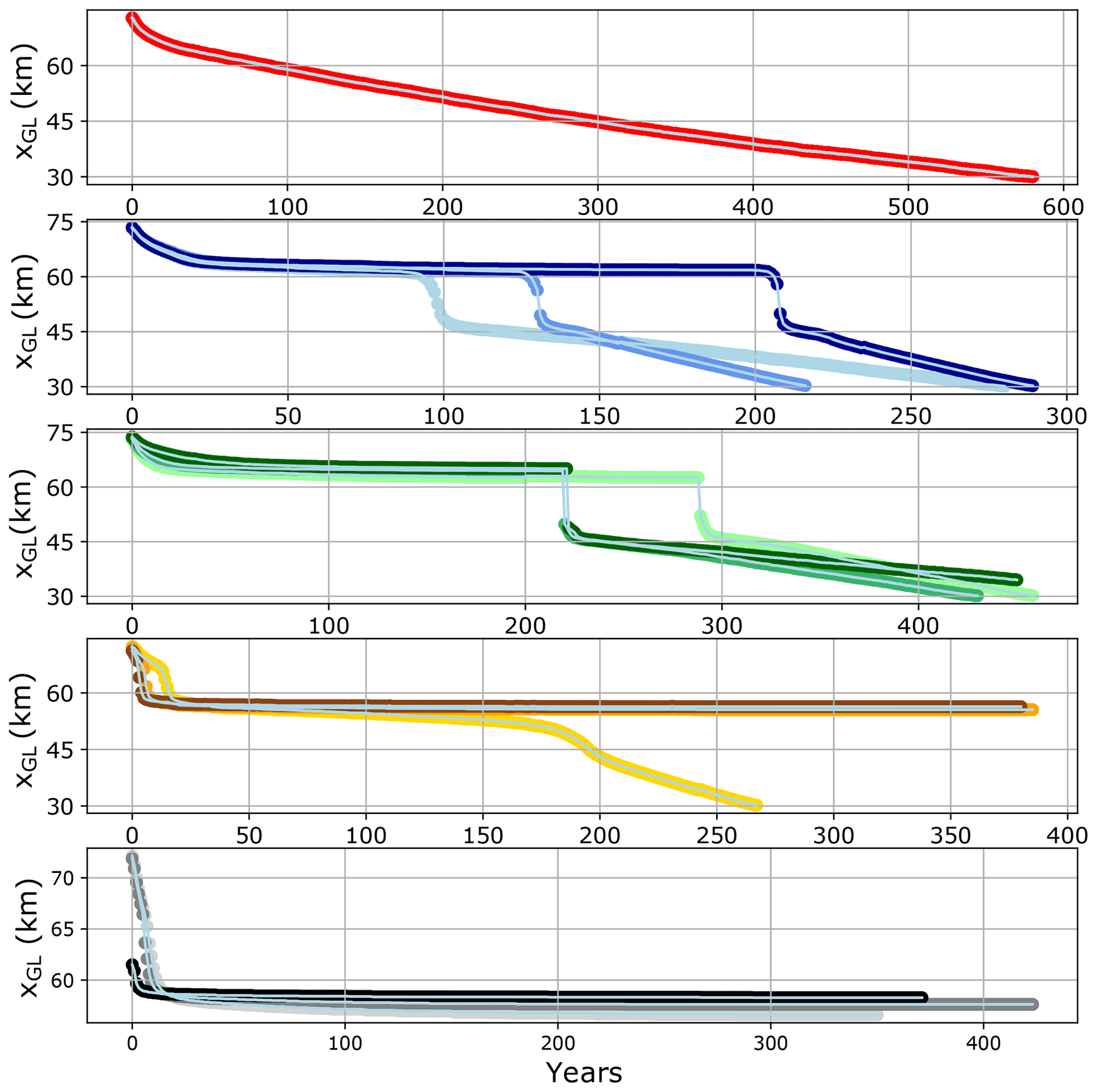
Figure A1 Grounding line position over time for different fjord geometries and magnitudes (for color code refer to Fig. 2). From top to bottom: linear fjord reference run, embayments, depressions, bottlenecks, bumps.

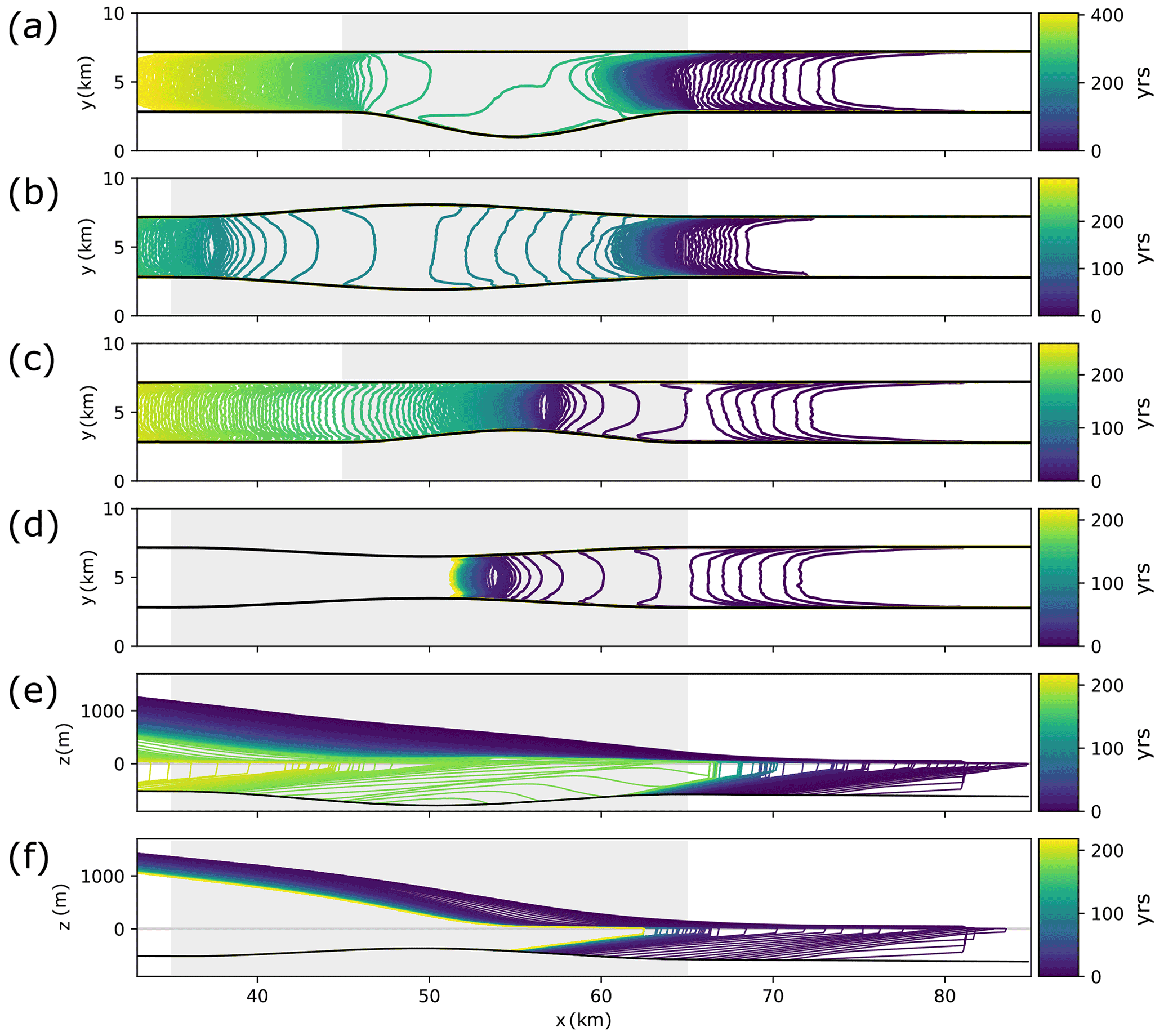
Figure A2 Retreat through asymmetric and longer perturbations. Annual grounding lines for lateral perturbations (a–d), annual profiles through glaciers for basal perturbations (e, f). Geometries shown are (with names referring to Table 2): (a) ByH1800_asy, (b) ByH900_lon, (c) ByH-900_asy, (d) ByH-675_lon, (e) BuH-240_lon, (f) BuH180_lon. Shaded areas indicate extent of geometric perturbation.

Figure A3 Stress fields in asymmetric and longer geometries. Lateral shear stress gradients for lateral perturbations (a, b, c, d) and longitudinal stress gradients for basal perturbations (e, f).

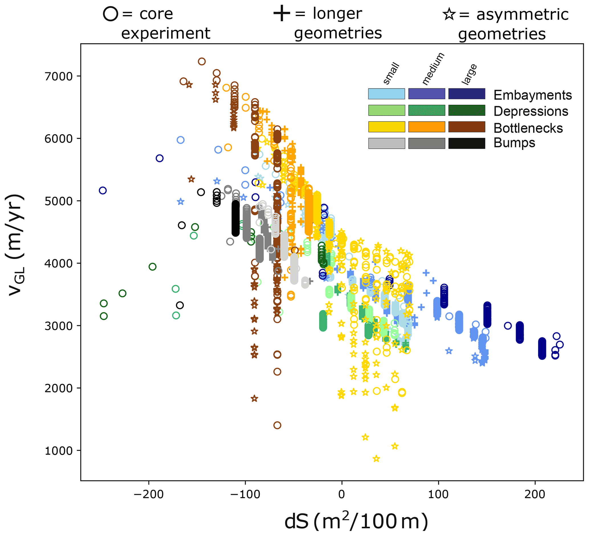
Figure A4 Correlation of v_GL over dS for all geometries including asymmetric and longer ones. Differences between this relationship and the relationship $Q_{\mathrm{GL}}/S$ over dS originate from time instances when the ice front is grounded well above flotation (and therefore $v_{\mathrm{GL}}\mathrm{not}\propto Q_{\mathrm{GL}}/S$) and because we measure v_GL only along the central flow line of the glacier.

Figure A5 Correlation of dGL over S including depressions.