Modelling surface temperature and radiation budget of snow-covered complex terrain

The surface temperature controls the temporal evolution of the snowpack, playing a key role in metamorphism and snowmelt. It shows large spatial variations in mountainous areas because the surface energy budget is affected by the topography, for instance because of the modulation of the short-wave irradiance by the local slope and the shadows and the short-wave and long-wave re-illumination of the surface from surrounding slopes. These topographic effects are often neglected in large-scale models considering the surface to be flat and smooth. Here we aim at estimating the surface temperature of snow-covered mountainous terrain in clear-sky conditions in order to evaluate the relative importance of the different processes that control the spatial variations. For this, a modelling chain is implemented to compute the surface temperature in a kilometre-wide area from local radiometric and meteorological measurements at a single station. The first component of this chain is the Rough Surface Ray-Tracing (RSRT) model. Based on a photon transport Monte Carlo algorithm, this model quantifies the incident and reflected short-wave radiation on every facet of the mesh describing the snow-covered terrain. The second component is a surface scheme that estimates the terms of the surface energy budget from which the surface temperature is eventually estimated. To assess the modelling chain performance, we use in situ measurements of surface temperature and satellite thermal observations (Landsat 8) in the Col du Lautaret area, in the French Alps. The results of the simulations show (i) an agreement between the simulated and measured surface temperature at the station for a diurnal cycle in winter within 0.2 ^∘C; (ii) that the spatial variations in surface temperature are on the order of 5 to 10 ^∘C in the domain and are well represented by the model; and (iii) that the topographic effects ranked by importance are the modulation of solar irradiance by the local slope, followed by the altitudinal variations in air temperature (lapse rate), the re-illumination by long-wave thermal emission from surrounding terrain, and the spectral dependence of snow albedo. The changes in the downward long-wave flux because of variations in altitude and the absorption enhancement due to multiple bounces of photons in steep terrain play a less significant role. These results show the necessity of considering the topography to correctly assess the energy budget and the surface temperature of snow-covered complex terrain.

1 Introduction

The snow cover is rarely flat and smooth on Earth. Undulations exist over a very large range of scales, from the centimetre to the kilometre scale. At the centimetre and metre scales, ripples, snow dunes, and erosion features (sastrugi) formed by wind usually coexist (Filhol and Sturm, 2015). Penitents (spike formations of snow and ice; Lliboutry, 1954) are also found in some particular conditions. At the decametre to kilometre scale range, the snow surface topography is mostly determined by the underlying soil or ice topography (Revuelto et al., 2018). Because of all these undulations, the surface temperature can vary by several degrees Celsius across a study area, even without significant differences in the near-surface meteorological forcing (incident radiation, wind, air temperature, humidity). Terrain slope and orientation and the presence of facing neighbouring slopes cause significant variations in the surface energy budget and more specifically in the radiative components. An abundant amount of literature has investigated how the short-wave (SW) and long-wave (LW) radiation is distributed across a complex terrain (Marks and Dozier, 1979; Duguay, 1993; Plüss and Ohmura, 1997), often for applications in mountainous areas.

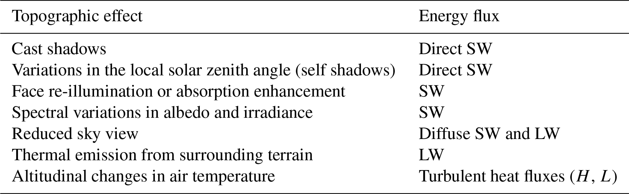
Figure 1 Illustration of the topographic effects considered in this study. They are summarized in Table 1. The colour code in the scheme that illustrates the lapse rate effect means decreasing temperatures with increasing elevation.

This study aims at quantifying the relative importance of a series of topographic effects that control the surface energy budget and the surface temperature. These effects are illustrated in Fig. 1 and summarized in Table 1. The first effect is the combination of the shadowing from local horizons (cast shadows) and the modulation of the direct solar irradiance depending on the face slope and aspect relative to the sun's position. This modulation depends on the local solar zenith angle (SZA). Self-shadowing occurs when the face completely turns away from the sun (local SZA <0 or >90^∘). Chen et al. (2013) accounted for this first effect, all the other terms of the energy budget being calculated as for flat terrain. This approximation is called “small slope approximation” by Picard et al. (2020) and is valid for gentle slopes up to ≈20^∘.

Arnold et al. (2006) investigated the topographic parameters controlling the surface energy balance on an Arctic glacier. Their model takes into account not only the local SZA and cast shadows for direct SW radiation, but also the sky-view factor for the diffuse SW and sky LW radiation. The model additionally accounts for LW radiation from the surrounding slopes by assuming an average surface temperature, a simplification with respect to the reality where each face may have a different temperature. The model evaluated with measured melt rate in different parts of the glacier performs well (correlation coefficient r≈0.85 for the majority of the melt season). The topographic effects ranked by importance are first shadows, followed by the local SZA and the sky-view factor. Olson et al. (2019) confirmed this ranking by studying the first two effects. LW emission by surrounding slopes can be a significant term in a steep topography. At larger scales (kilometre), Yan et al. (2016) showed that neglecting these topographic effects may induce errors of up to 100 W m⁻² for the modelled net LW flux.

Absorption enhancement due to multiple scattering within the topography is an additional effect, particularly important in steep terrains. It is indeed likely that the incident photons in such a terrain encounter more than one bounce between the terrain slopes before escaping to the sky or being absorbed in the snow. The total probability of absorption of a given incident photon is thereby increased at every bounce compared to a flat or smooth surface where at most one bounce occurs (Warren et al., 1998). Larue et al. (2020) experimentally quantified this effect by measuring spectral albedo over artificial rough surfaces, showing a decrease in albedo (i.e. increase in absorption) on the order of 0.03–0.08 in the visible and near-infrared compared to a smooth surface. This range was confirmed in the SW using optical models for rough surfaces (Warren et al., 1998; Leroux and Fily, 1998; Lhermitte et al., 2014). For real 3D terrains, ray-tracing and Monte Carlo techniques can take into account this effect (Larue et al., 2020) at the expense of intensive computation. Lee et al. (2013) used similar methods to show the impact of including the topography on the surface radiation budget over the whole Tibetan Plateau. They found differences of ≈14 W m⁻² with respect to a flat-surface calculation. A simpler approach to account for multiple bounces is to add a mean contribution coming from neighbouring slopes by assuming that they are illuminated as if they were flat (Lenot et al., 2009; Olson et al., 2019). This contribution requires a value representing the effective albedo of neighbouring terrain and is modulated by the sky-view factor of the slope. It is important to note that the absorption enhancement is not uniform; it is usually stronger in the valleys (trapping effect) than near the summits of the topography (Lliboutry, 1954).

In addition, most models cited above consider only broadband SW fluxes, neglecting the spectral dependence of snow albedo and incident radiation. The probable consequence is an inaccurate estimation of the absorption enhancement due to neglecting the large difference in albedo between the visible and the near-infrared. In the visible, the albedo is high (typically over 0.95), implying intense multiple scattering but extremely weak absorption. In contrast, the albedo is lower in the near-infrared and closer to the optimal albedo for enhancement (0.5), where multiple scattering and absorption are balanced (Warren et al., 1998).

The turbulent heat fluxes are important in the surface energy budget (Brun et al., 1989), in particular during nights, as they balance the radiative cooling of the surface. These fluxes are difficult to parameterize when only a few in situ measurements are available (Martin and Lejeune, 1998; Pomeroy et al., 2016). In complex terrain, their spatial and temporal variations are mostly determined by the wind distribution around the relief and by the change in air temperature with elevation (Rotach and Zardi, 2007).

The most advanced model to simulate surface temperature in a mountainous area is – to our knowledge – a commercial product (Adams et al., 2009, 2011) which includes not only a comprehensive energy budget modelling (including absorption enhancement and emission by faces), but also radiation penetration in the snow, different types of surface (snow, rock, tree), and the heat diffusion in the snow to describe the full temperature profile in the snowpack. The precise equations and approximations are however not known. In a study case in south-western Montana, USA, the model predicts spatial variations in temperature between −15 and 0 ^∘C at 14:00 local time, with most of these variations being primarily explained by terrain type. This non-exhaustive review of approximations and models in the literature highlights the various effects related to the topography, the large number of possible approximations, and the different scales of application (metre-scale roughness and complex-terrain scales).

Table 1 Several effects relevant to short-wave (SW), long-wave (LW), and turbulent heat flux calculation in complex terrains. Other effects such as those involving the atmosphere are beyond the scope of this study.

To investigate the relative importance of the topographic effects, this study aims at modelling the snow surface temperature variations in a mountainous area from radiometric and meteorological measurements at a single point. The modelling chain includes a 3D radiative transfer model, the Rough Surface Ray-Tracing (RSRT) model (Larue et al., 2020), to compute the incident and reflected SW radiation. The model launches a set of photons to the snow surface described by a triangular mesh (i.e. a connected set of triangular facets) that can be derived easily from a digital elevation model (DEM). Its spatial resolution limits the scope of this study to topography at the decametre to kilometre scale range. The RSRT simulation results are then used in a surface scheme (RoughSEB model) to compute the net SW and LW radiation and the turbulent heat fluxes on each facet as a function of the facet surface temperature. The surface temperature is eventually deduced by closure of the energy budget. To assess the modelling chain performance, satellite thermal infrared observations from Landsat 8 are used. The topographic effects that are taken into account in this study can be disabled or modified when needed in order to quantify their relative importance by measuring the impact on the surface temperature. This study is applied at the Col du Lautaret area (French Alps), and we mostly consider clear-sky conditions since they tend to maximize the topographic effects compared to diffuse conditions. Section 2 provides the model description as well as the method for retrieving surface temperature from satellite images and a description of the study area. Results are shown in Sect. 3 and discussed in Sect. 4. The conclusions are presented in Sect. 5.

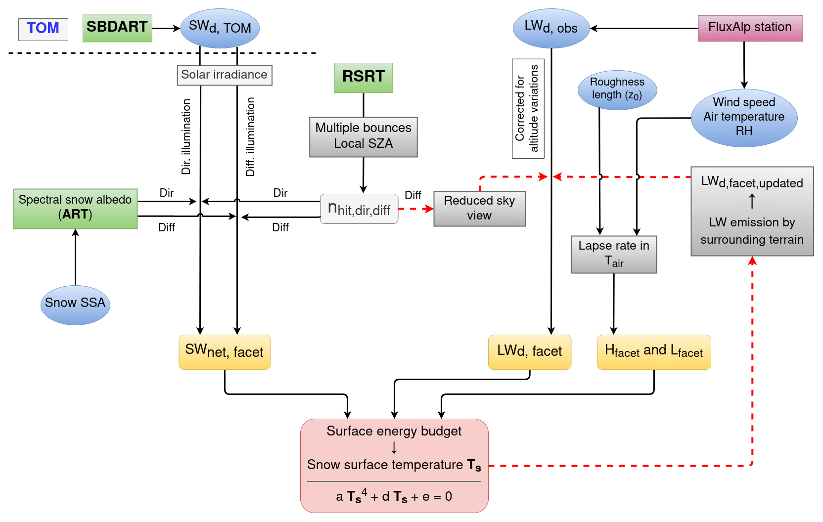
Figure 2 Flowchart of the modelling chain to estimate snow surface temperature. TOM (top of mountains) is the horizontal above the highest point in the study area. The involved models are in green, the terms of the surface energy budget are in orange, the needed inputs are in blue, and the topographic effects are in grey. The dashed red lines indicate the two-step iterative process to compute the downward LW flux.

2 Methods and materials

2.1 The RoughSEB model

Snow surface temperature (T_s) is obtained by solving the surface energy budget equation for each facet of the modelled snow surface. The energy budget comprises (Arya, 1988) (i) the net radiation fluxes, which are split into the contributions of the short-wave radiation from 0.3 to 4 µm (SW_net) and the long-wave radiation from 3 to 100 µm (LW_net); (ii) the sensible heat flux (H), which arises as a result of the exchange of heat between the surface and the air just above; (iii) the latent heat flux (L) resulting from water state changes (sublimation or condensation) at the surface and exchange with the air above; and (iv) the ground heat flux (G), which is transferred to the snowpack and leads to a change in snow temperature or melt. Here, we assume below-freezing temperature so that melt is not involved. The sum of these fluxes is null according to the first principle of thermodynamics since the surface has no internal enthalpy:

$$\begin{array}{}\text{(1)}& {\text{SW}}_{\text{net}}+{\text{LW}}_{\text{net}}\left(T_{\text{s}}\right)+H\left(T_{\text{s}}\right)+L\left(T_{\text{s}}\right)+G=\mathrm{0}.\end{array}$$

Each term of this equation is estimated with a chain of existing and new models depicted in Fig. 2. All the constant terms are calculated for each facet (hereafter noted with the subscript f), and the rest are calculated as a function of the facet temperature. The snow surface temperature is eventually estimated for each facet of the modelled surface by closure of the energy budget (Sect. 2.1.4).

The computation of the SW_net radiation (Sect. 2.1.1) involves (i) the Santa Barbara DISORT Atmospheric Radiative Transfer model (SBDART; Ricchiazzi et al., 1998), an atmospheric model that simulates the incoming spectral irradiance above the studied area (top of mountains, TOM), and (ii) the RSRT model (Larue et al., 2020), based on a Monte Carlo photon-tracking algorithm that computes the path of the photons launched towards the surface and allows the consideration of the modulation of SW radiation by the terrain slope and aspect. The simulations are done separately for the direct and diffuse components of the short-wave irradiance (noted with subscripts dir and diff). Moreover, the atmospheric effects (i.e. atmospheric attenuation, clouds) are neglected within the studied domain (between the surface and TOM). The scene is considered to be covered by pure snow (i.e. no impurities), which applies in winter. The calculation of the LW_net radiation (Sect. 2.1.2) needs the downwelling LW flux, measured by a local station and corrected for altitude variations within the domain. It is subsequently updated by accounting for the reduced sky-view factor of each facet and the thermal emission of surrounding terrain. The turbulent heat fluxes (H and L) are computed with a simplified approach (Sect. 2.1.3) that involves common in situ meteorological measurements (i.e. air temperature, wind speed, and relative humidity) and introduces a lapse rate effect.

2.1.1 Calculation of the short-wave radiation fluxes

The calculation of the SW_net radiation takes into account (i) the topographic effects affecting the SW radiation and (ii) the spectral dependence of snow albedo and incident solar irradiance. The aim is to compute it on every facet f due to the direct and diffuse components of the solar irradiance:

$$\begin{array}{}\text{(2)}& {\displaystyle }{\text{SW}}_{\text{net},f}\left({\mathit{\theta }}_{\text{s}}\right)& {\displaystyle }={\text{SW}}_{\text{net, dir},f}\left({\mathit{\theta }}_{\text{s}}\right)+{\text{SW}}_{\text{net, diff},f}\text{(3)}& {\displaystyle }{\text{SW}}_{\text{net, dir},f}\left({\mathit{\theta }}_{\text{s}}\right)& {\displaystyle }=\underset{{\mathit{\lambda }}_{\mathrm{0}}}{\overset{{\mathit{\lambda }}_{\mathrm{1}}}{\int }}{\text{A}}_{\text{dir},f}(\mathit{\lambda },{\mathit{\theta }}_{\text{s}}){\text{I}}_{\text{dir}}\left(\mathit{\lambda }\right)\mathrm{d}\mathit{\lambda }\text{(4)}& {\displaystyle }{\text{SW}}_{\text{net, diff},f}& {\displaystyle }=\underset{{\mathit{\lambda }}_{\mathrm{0}}}{\overset{{\mathit{\lambda }}_{\mathrm{1}}}{\int }}{\text{A}}_{\text{diff},f}\left(\mathit{\lambda }\right){\text{I}}_{\text{diff}}\left(\mathit{\lambda }\right)\mathrm{d}\mathit{\lambda },\end{array}$$

where the direct and diffuse components of the absorbed SW radiation by every facet are computed using (i) an absorption coefficient A_{dir, diff,f}, derived from the RSRT model, and (ii) the spectral irradiance coming from the sky I_{dir, diff}(λ), issued from the SBDART model. The integration is between λ₀=300 nm and λ₁=4200 nm to cover all the solar radiation spectrum.

A direct way to compute the absorbed SW radiation by each facet would be to use the ray-tracing RSRT model to trace many photons for every wavelength in the solar spectrum. Nevertheless, with millions of facets and hundreds of wavelengths, this approach would imply an enormous computational cost due to the inefficiency of the Monte Carlo ray-tracing method. To overcome this, we take advantage of the result of the RSRT model to account for multiple bouncing. In this model, each launched photon has an initial propagation direction specified by the zenith and azimuth angles and a random initial position above the mesh. The intersection between the photon direction and the mesh surface is first calculated. Then, to simulate a Lambertian reflection, the change in direction is taken randomly from the cosine-weighted hemispherical distribution. The algorithm iterates as long as the photon propagates from facet to facet and stops only when the photon escapes from the domain or when a maximum number of bounces is reached (noted n_max). No albedo and no absorption are involved at this stage; RSRT only computes possible geometric trajectories of photons in the given mesh. The number of photons launched is 4×10⁸, and edge effects are avoided by excluding the outermost 15 % of the mesh area.

The RSRT model records the number of times photons have hit a given facet as a function of the bounce order of the photon (first reflection, second reflection, …). It is hereafter noted $n_{\text{hit, d},f}^{\left(i\right)}$ and corresponds to the proportion of photons that directly hit the facet at their ith reflection (from i=0, and d is dir or diff depending on the illumination conditions – direct or diffuse). Assuming that the area has a uniform albedo (same snow properties everywhere in the domain) and that the reflections are Lambertian, the absorption coefficient A_{dir, diff,f} is computed by taking into account (i) the spectral dependence of snow albedo and (ii) the fact that the illumination received by each facet is the sum of the illumination from photons at their first reflection and the multiple bounce contribution, considered to be diffuse illumination from photons at their second reflection, third reflection, etc. The coefficient is determined with

$$\begin{array}{}\text{(5)}& {\displaystyle }\begin{array}{rl}{A}_{\text{dir},f}(\mathit{\lambda },{\mathit{\theta }}_{\text{s}})& =\left[\mathrm{1}-{\mathit{\alpha }}_{\text{dir}}(\mathit{\lambda },{\mathit{\theta }}_{\text{s}})\right]n_{\text{hit, dir},f}^{\left(\mathrm{0}\right)}\\ & +\left[\mathrm{1}-{\mathit{\alpha }}_{\text{diff}}\left(\mathit{\lambda }\right)\right]{\mathit{\alpha }}_{\text{dir}}(\mathit{\lambda },{\mathit{\theta }}_{\text{s}})\\ & \cdot \sum _{i=\mathrm{1}}^{i=n_{\max }}{\mathit{\alpha }}_{\text{diff}}^{i-\mathrm{1}}\left(\mathit{\lambda }\right)n_{\text{hit, dir},f}^{\left(i\right)}\end{array}\text{(6)}& {\displaystyle }{A}_{\text{diff},f}\left(\mathit{\lambda }\right)=\left[\mathrm{1}-{\mathit{\alpha }}_{\text{diff}}\left(\mathit{\lambda }\right)\right]\sum _{i=\mathrm{0}}^{i=n_{\max }}{\mathit{\alpha }}_{\text{diff}}^i\left(\mathit{\lambda }\right)n_{\text{hit, diff},f}^{\left(i\right)},\end{array}$$

where θ_s is the local solar zenith angle, and α_{dir, diff}(λ,θ_s) is the snow spectral albedo under direct and diffuse illumination. Here, these albedos are computed using the asymptotic radiative transfer (ART) theory (Kokhanovsky and Zege, 2004), whose formulation is presented in the Appendix A1. The calculation needs the snow specific surface area (SSA) as input. If not specified, a standard value of 20 m² kg⁻¹ is assumed in the modelling.

The spectral irradiance coming from the sky I_{dir, diff}(λ) is computed with the SBDART model. This model computes the atmospheric transmission and scattering (Mie theory). The simulations are run in the spectral range 300–4200 nm by steps of 3 nm. Here, a generic mid-latitude winter atmospheric profile is assumed, and the aerosol optical depth at 550 nm is 0.08 (“rural” profile in SBDART). The elevation is 2052 m a.s.l. (see Sect. 2.2), and solar zenith and azimuth angles correspond to the desired date and time.

The net broadband SW radiation of each facet is eventually calculated by means of Eq. (2).

2.1.2 Long-wave radiation fluxes

To compute the incident LW flux from the atmosphere on each facet, we first apply a local correction to the observed downward LW flux (noted LW_{d, obs}), measured in a single point of the domain (Sect. 2.2). This correction takes into account the LW variations in altitude over the whole domain using the same approach as in Arnold et al. (2006). The correction consists of deriving an “effective emissive temperature” of the sky (noted T_{sky, obs}) from the measured LW flux with the Stefan–Boltzmann equation. This temperature is corrected for changes in elevation by introducing the lapse rate Γ:

$$\begin{array}{}\text{(7)}& {\displaystyle }{\text{LW}}_{\text{d, obs}}& {\displaystyle }=\mathit{\sigma }{T}_{\text{sky, obs}}^{\mathrm{4}}\text{(8)}& {\displaystyle }{T}_{\text{sky},f}& {\displaystyle }=T_{\text{sky, obs}}+\mathrm{\Gamma }(z_f-z_{\text{obs}}),\end{array}$$

with σ the Stefan–Boltzmann constant and where T_sky,f is the effective emissive temperature of the atmosphere above each facet. We choose $\mathrm{\Gamma }=-\mathrm{6.5}$ ${}^{\circ }\mathrm{C}{\mathrm{km}}^{-\mathrm{1}}$, the environmental lapse rate as defined in the International Standard Atmosphere (ISO 2533:1975, 1975). The downwelling LW flux incident on each facet (LW_d,f) is then recalculated with the Stefan–Boltzmann equation:

$$\begin{array}{}\text{(9)}& {\text{LW}}_{\text{d},f}=\mathit{\sigma }{T}_{\text{sky},f}^{\mathrm{4}}.\end{array}$$

In complex terrain facets receive radiation not only from the atmosphere but also from the surrounding slopes. Computing this contribution requires the facet surface temperature, which is precisely unknown. We proceed by iteration in two steps: in the first step, we neglect the thermal emission from the surrounding facets. This leads to a first estimate of the surface temperature (Sect. 2.1.4) that is then used in the second step to account for the emission of surrounding terrain. The average upwelling LW flux from each facet (LW_{u, scene average}) is computed from the average surface temperature of the whole domain with the Stefan–Boltzmann equation. This thermal emission is a constant; we neglect the possible variations in temperature around each facet. The updated downwelling LW flux on each facet is eventually calculated with

$$\begin{array}{}\text{(10)}& {\text{LW}}_{\text{d},f,\mathrm{updated}}=V_f{\text{LW}}_{\text{d},f}+(\mathrm{1}-V_f){\text{LW}}_{\text{u, scene average}},\end{array}$$

where V_f is the sky-view factor calculated with RSRT. V_f is different for each facet: those in the valley receive more LW radiation from the surrounding slopes than facets at the summits of the domain. The sky-view factor is indeed equal to the proportion of the launched photons hitting a facet on their first bounce in diffuse illumination, namely $V_f=n_{\text{hit, diff},f}^{\left(\mathrm{0}\right)}$.

The upwelling long-wave radiation, LW_u,f, is determined by the Stefan–Boltzmann law:

$$\begin{array}{}\text{(11)}& {\text{LW}}_{\text{u},f}=\mathit{ϵ}\mathit{\sigma }{T}_{\text{s}}^{\mathrm{4}}+(\mathrm{1}-\mathit{ϵ}){\text{LW}}_{\text{d},f},\end{array}$$

with snow emissivity ϵ=0.98 and T_s the snow surface temperature of the facet.

2.1.3 Turbulent heat fluxes

While the main focus of this work is on the role of the topographic effects controlling the radiation budget of the surface, the turbulent heat fluxes also need to be assessed to close the surface energy budget. We follow a simple modelling approach; potential improvements are left to further work in the future. The sensible and latent heat fluxes are calculated following the one-level approach:

$$\begin{array}{}\text{(12)}& {\displaystyle }{H}_f& {\displaystyle }={\mathit{\rho }}_{\text{air}}{c}_{p,\text{air}}{C}_{\text{H}}U(T_{\text{s}}-T_{\text{air}})\text{(13)}& {\displaystyle }{L}_f& {\displaystyle }=L_s{\mathit{\rho }}_{\text{air}}{C}_{\text{H}}U\cdot \left(q_{\text{sat}}\right(T_{\text{s}},P_{\text{s}})-q_{\text{air}}),\end{array}$$

where ρ_air and c_p,air are the density and heat capacity of the air; U is the wind speed, T_air is the air temperature; L_s is the sublimation heat; q_sat(T_s,P_s) is the saturation specific humidity at the snow surface, with surface temperature T_s and pressure P_s; and q_air is the specific humidity at the level where air temperature and humidity are measured. C_H is a surface exchange coefficient which in principle depends on atmospheric stability. For the sake of simplicity, a neutral situation is considered here. C_H therefore depends only on the aerodynamic roughness length z₀, assumed constant across the domain and equal to 10⁻³ m following previous works (Brock et al., 2006). The expression of this coefficient is provided in the Appendix A2, and the values of the defined symbols are presented in Table B1. The air temperature and wind speed are taken from the meteorological station (Sect. 2.2). T_air accounts for the variations in altitude within the domain in a similar way as the downward LW flux (Sect. 2.1.2), via a lapse rate effect (Eq. 8). Wind speed and relative humidity are however considered constant. Note that the specific humidity is deduced from the relative humidity and air temperature, so it indirectly depends on altitude.

The ground heat flux (G) is neglected here as the snowpack is considered thermalized. We assume that no energy is exchanged with the snowpack, which is checked in the discussion (Sect. 4.2).

2.1.4 Snow surface temperature estimation

The equation of the surface energy budget (Eq. 1) with explicit T_s dependencies is

$$\begin{array}{}\text{(14)}& \begin{array}{rl}{\text{SW}}_{\text{net},f}& +{\text{LW}}_{\text{d},f,\mathrm{updated}}-{\text{LW}}_{\text{u},f}\left(T_{\text{s}}^{\mathrm{4}}\right)\\ & +H_f\left(T_{\text{s}}\right)+L_f\left(q_{\text{sat}}\left(T_{\text{s}}\right)\right)=\mathrm{0}.\end{array}\end{array}$$

The equation is solved to determine the unknown T_s for each facet f. However this equation is non-linear due to the $T_{\text{s}}^{\mathrm{4}}$ term (upwelling LW radiation) and the complex dependence of the saturation specific humidity at the surface to T_s. Solving such an equation for millions of facets can be computationally intensive. To avoid this issue, we linearize the specific humidity at saturation about T_air, as in Essery and Etchevers (2004):

$$\begin{array}{}\text{(15)}& q_{\text{sat}}(T_{\text{s}},P_{\text{s}})=q_{\text{sat}}(T_{\text{air}},P_{\text{s}})+(T_{\text{s}}-T_{\text{air}})\cdot q_{\text{sat}}^{\prime }(T_{\text{air}},P_{\text{s}}),\end{array}$$

where

$$\begin{array}{}\text{(16)}& q_{\text{sat}}^{\prime }(T_{\text{air}},P_{\text{s}})=\left({\displaystyle \frac{q_{\text{sat}}(T_{\text{air}},P_{\text{s}})-q_{\text{sat}}(T_{\text{air}}-\mathrm{\Delta }T,P_{\text{s}})}{\mathrm{\Delta }T}}\right),\end{array}$$

with ΔT=5 K. The simplified surface energy budget equation eventually becomes a quartic equation for T_s of the form

$$\begin{array}{}\text{(17)}& a{T}_{\text{s}}^{\mathrm{4}}+d{T}_{\text{s}}+e=\mathrm{0},\end{array}$$

where a, d, and e are a constant (for each facet). The general solution (Neumark, 1965) of this equation is shown in the Appendix A3. The evaluation of this equation for a large number of facets is computationally efficient compared to using a non-linear optimization solver.

Figure 3 Location of the study area around the Col du Lautaret alpine site. The blue rectangle in (a) represents the extension of the study area, shown in (b). The domain is generated from the RGE ALTI®Version 2.0 digital elevation model (DEM) provided by IGN France at a spatial resolution of 5 m and resampled to 10 m for this study. Slope angle is represented by the intensity of the colour.

2.2 Study area and in situ measurements

Figure 3 shows the study area. It is located around the Lautaret mountain pass in the French Alps (45.0^∘ N, 6.4^∘ E). This area is of interest to study surface temperature as it features both north- and south-facing slopes that are spaced by a few hundred metres. It also contains smaller-scale rugged terrain covering the rest of orientations and promoting re-illumination. The size of the area is ≈50 km², and the range of altitudes spans from 1640 to 3220 m a.s.l. The predominant orientation is south-south-west-, followed by north-north-east-facing terrain, and the slope varies mainly between 15 and 40^∘. Protruding vegetation is rare in the study area in winter and is neglected here. We assume that the snow cover is 100 %. The mesh required for simulations was built from the RGE ALTI^® Version 2.0 digital elevation model (DEM) provided by IGN France (IGN, 2021), acquired using radar techniques in 2009. Its coordinate reference system is Lambert 93 (EPSG: 2154), and the original spatial resolution was 5 m. It was however resampled to 10 m to limit computational cost. To create the mesh, the centre of each pixel is taken as a vertex. Each vertex is then connected to their four closest neighbours, which eventually leads to two triangular facets shared by the same vertex.

The study area includes the measurement station FluxAlp (45.0413^∘ N, 6.4106^∘ E), located at 2052 m a.s.l. This station collects meteorological and radiometric observations. Radiation fluxes are measured with a Kipp & Zonen CNR4 radiometer with a spectral range of 0.3–2.8 µm in the SW and 4.5–42 µm in the LW. The data needed as input for the modelling chain are issued from here (air temperature, wind speed, relative humidity, and downwelling LW radiation flux). All measurements are averaged over 30 min; i.e. a measurement at 10:30 UTC is the average of the period 10:00–10:30 UTC. The upwelling LW measurements at FluxAlp are used to assess the modelled surface temperature at the station point.

Manual measurements of surface snow SSA for two consecutive winter seasons (2016/2017 and 2017/2018) have been collected occasionally (Tuzet et al., 2020) a few metres around the FluxAlp station. The measurements were collected with the DUFISSS instrument (Gallet et al., 2009) during the first season and with the Alpine Snowpack Specific Surface Area Profiler (ASSSAP; a lighter version of the POSSSUM instrument; Arnaud et al., 2011) during the second season. These measurements have an estimated uncertainty of 10 %.

2.3 Surface temperature retrieval with Landsat 8 observations

Spatial variations in surface temperature are retrieved from satellite observations. The two thermal bands (thermal infrared sensor, TIRS – Bands 10 and 11) onboard Landsat 8 cover the spectrum at around 10.6 and 12.51 µm, with a spatial resolution of 100 m (resampled by cubic convolution methods to 30 m in the product) and a 16 d repeat cycle. Different methods to correct atmospheric effects have been implemented in order to retrieve land surface temperature (LST hereafter): split-window methods (Jin et al., 2015), mono-window techniques (Tardy et al., 2016), or single-channel approaches (Jiménez-Muñoz and Sobrino, 2003). Soon after the launch of Landsat 8, stray light was observed on thermal data (Montanaro et al., 2014) due to scattering of outer radiance in Band 11. Methods based on only one band are therefore suggested. The single-channel approach proposed by Jiménez-Muñoz and Sobrino (2003) approximates the atmospheric functions from the atmospheric water vapour content (w; in g cm⁻²). Cristóbal et al. (2018) presented an improved single-channel method dependent on not only water vapour content but also on near-surface air temperature (T_a). Figure 4 shows the flowchart to retrieve LST from satellite observations, following Cristóbal et al. (2018).

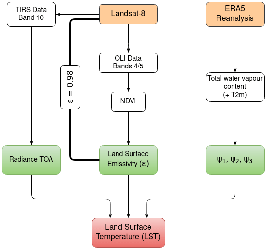
Figure 4 Workflow to retrieve land surface temperature from Landsat 8 thermal observations with a single-channel approach.

Both the single-channel method (SC method; Jiménez-Muñoz and Sobrino, 2003) and the improved single-channel method (iSC method; Cristóbal et al., 2018) have been implemented in this study. LST is calculated for each pixel by applying the radiative transfer equation to a sensor channel (Eqs. 1 to 3 in Cristóbal et al., 2018), which eventually leads to

$$\begin{array}{}\text{(18)}& \text{LST}=\mathit{\gamma }\cdot \left[{\mathit{\epsilon }}^{-\mathrm{1}}({\mathit{\psi }}_{\mathrm{1}}\cdot L_{\text{sensor},\mathit{\lambda }}+{\mathit{\psi }}_{\mathrm{2}})+{\mathit{\psi }}_{\mathrm{3}}\right]+\mathit{\delta },\end{array}$$

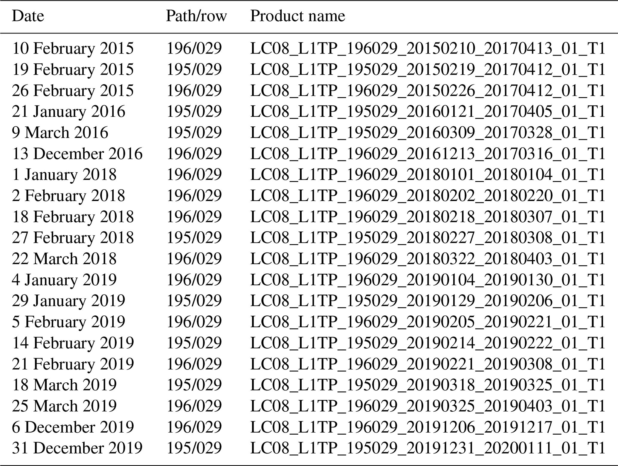
where γ and δ are constants that depend on the top-of-atmosphere radiance (L_sensor,λ) and the brightness temperature of the pixel, ε is the emissivity of the pixel, and ψ_i represents the atmospheric parameterized functions. More details are shown in Appendix A4 for completeness. The emissivity is considered equal to 0.98 in the whole scene, in line with our modelling chain. Water vapour and near-surface air temperature data come from the ERA5 Reanalysis dataset (Hersbach et al., 2018). They are taken from the closest grid point. In order to cover a large range of solar zenith angles, a total of 20 cloudless thermal images from different winter dates were selected, from February 2015 to December 2019 (list in Appendix C). The acquisition times of Landsat 8 observations (10:17 or 10:23 UTC depending on the scene) and in situ measurements (10:30 UTC, averaged over the previous 30 min) are considered to be equivalent. Among the selected clear-sky days, 4 of them have accompanying manual measurements of snow SSA (Tuzet et al., 2020). These are 2 February 2018, 18 February 2018, 27 February 2018, and 22 March 2018, with snow SSA of 47, 45, 53, and 32 m² kg⁻¹, respectively.

The Landsat Collection 2 surface temperature product recently made public is also considered here. It is compared to the results of the aforementioned LST retrieval methods in our case of study.

3 Results

The spatially resolved LST observations from Landsat 8 are first assessed in the study area before the evaluation of the model simulations against the local measurements and the satellite observations. Finally the relative importance of the topographic effects on surface temperature is quantified.

3.1 Surface temperature observations from Landsat 8

The surface temperature observations from Landsat 8 (LST) are compared to the in situ FluxAlp measurements (Fig. 5a). The Landsat 8 surface temperature is extracted from the pixel covering the FluxAlp station location from all the 20 thermal images. Both the single-channel (SC) method and the improved single-channel (iSC) method show better estimations at the FluxAlp station than the official Collection 2 surface temperature product (−3.5 ^∘C underestimation). As a result, we exclude this latter dataset from further analysis. The iSC method provides generally higher temperatures than the SC method, with a mean bias of −1.3 and −2.0 ^∘C, respectively. Its total error is of 2.0 ^∘C RMS, dominated by the bias (2.6 ^∘C for the SC method). The improved single-channel method shows slightly more accurate results, and it is used in the following to evaluate the estimation of snow surface temperature by the modelling chain.

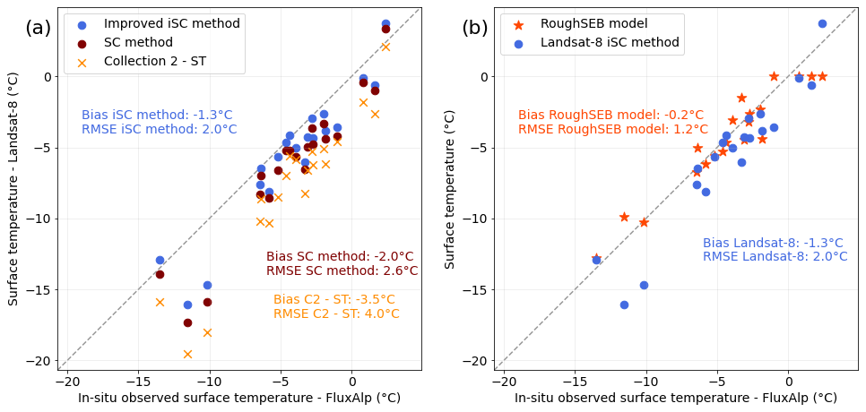
Figure 5 Landsat-8-retrieved surface temperature as a function of surface temperature measurements at the FluxAlp station (a) using the iSC method (blue) and the SC method (brown). The Collection 2 surface temperature product is shown in orange. (b) Simulated T_s by the model (red) and observed T_s by Landsat 8 (iSC method, blue). The 1:1 dashed line represents perfect agreement with in situ measurements.

3.2 Snow surface temperature simulations

3.2.1 Validation at the FluxAlp station

Figure 5b shows Landsat 8 observations and snow surface temperature simulations compared to the in situ measurements at FluxAlp. The RoughSEB model is in general in agreement with the satellite observations. Considering all the images, they differ by up to 1 ^∘C, the simulations being slightly warmer. The differences are however larger when considering the coldest cases, up to 5 ^∘C. The error in the simulations is lower, 1.2 ^∘C RMS (2.0 ^∘C for Landsat observations).

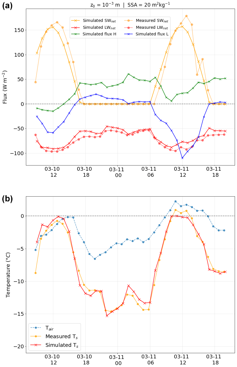
Figure 6 Simulation of the surface fluxes (a) and snow surface temperature (b) at the FluxAlp station for a ≈36 h long time series starting 10 March 2016. The radiative fluxes are compared to in situ measurements. All times are in UTC.

3.2.2 Evaluation of the diurnal cycle

The modelling chain to estimate T_s is evaluated over a diurnal cycle at the FluxAlp station (Fig. 6). A period of ≈36 h was selected after one of the Landsat 8 acquisition dates, starting at 09:00 UTC on 10 March 2016. This period featured stable conditions, and the sky was clear, except for a few minutes at the end of the period. Figure 6 (top) shows the temporal evolution of the radiative fluxes (SW_net and LW_net) and the turbulent fluxes (sensible heat flux H and latent heat flux L). The simulations are run hourly, with a constant SSA =20 m² kg⁻¹ and aerodynamic roughness length $z_{\mathrm{0}}={\mathrm{10}}^{-\mathrm{3}}$ m. The radiative fluxes are compared to the in situ measurements at the station, and the simulated turbulent heat fluxes are shown for completeness. It should be recalled that the simulations are run with a spectral range 300–4200 nm for the SW in order to cover the entire solar radiation spectrum. However, for a fair comparison with the measured SW_net, additional SW calculations are run in the same spectral range of the pyranometer (300–2800 nm). As measurements at the FluxAlp station are averaged over the preceding 30 min, a 15 min time shift is applied on the graph. The results show that the net short-wave flux is slightly underestimated except during the first hours of sunlight, when it is overestimated. The difference is almost negligible (<5 W m⁻²) around 10:00–10:30 UTC, which by chance corresponds to the Landsat 8 acquisition time. The underestimation leads to an overall bias over daytime of ≈5 W m⁻², while the net long-wave radiation flux is in general overestimated by ≈7 W m⁻². Figure 6 (bottom) shows the evolution of the simulated T_s over the same period compared to the in situ measurements. Observed air temperature is also shown for completeness. There is a good agreement between the simulations and the measurements, within 0.2 ^∘C (RMSE: 0.8 ^∘C). Surface temperature shows a diurnal cycle, where the melting point is barely reached in the early afternoon, and the lowest temperatures are reached at night. The bias in T_s towards the end of the afternoon could be explained by the balance between the underestimation of the net SW flux and the overestimation of the net LW flux. The slight variations in surface temperature (around 2 to 3 ^∘C) during the night are mainly driven by the balance between the long-wave radiation flux and the sensible heat flux, the other fluxes being negligible.

3.2.3 Evaluation of the spatial variations

To evaluate the spatial variations in T_s, the simulation corresponding to the Landsat 8 acquisition on 18 February 2018 is analysed here. It is chosen because in situ SSA measurements were available (Tuzet et al., 2020), allowing a more accurate estimate of the surface albedo. The SSA value is 45 m² kg⁻¹.

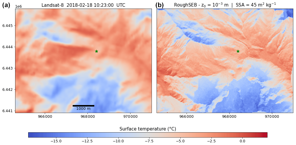
Figure 7 Surface temperature observed by Landsat 8 (a) and simulated by the RoughSEB model (b) in the Col du Lautaret area on 18 February 2018. The location of the FluxAlp station is highlighted by the green marker. Projection is Lambert 93 (EPSG: 2154), and the coordinates are in metres.

Figure 7 shows the spatial variations in snow surface temperature, observed by Landsat 8 (left) and simulated by the RoughSEB model (right). The variations are well represented by the model, with many similarities at all the scales across the domain. The small-scale variations are better resolved by the model as the spatial resolution is significantly higher (10 vs. 30 m for the satellite). This is in particular true in the northern area of the domain, which features a series of small valleys, showing a larger temperature gradient in the simulation. The model is slightly colder in the coldest areas (e.g. shadows in the southern area of the scene) as well as in the warmest areas around the FluxAlp station (green marker). As shown in Fig. 5b, the surface temperature does not differ significantly in the FluxAlp area.

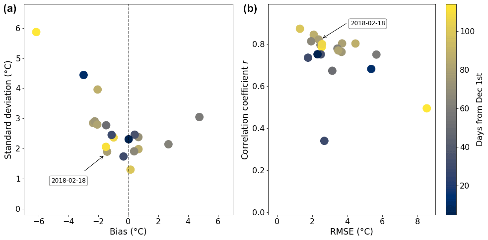
Figure 8 Comparison of the spatial variations in surface temperature between the simulations and the satellite observations for each date, computed considering the whole domain. (a) Mean bias and standard deviation of the differences. (b) RMSE and the correlation coefficient r.

Figure 8 (left) shows the bias and standard deviation of a pixel-to-pixel comparison between all the 20 satellite observations and the corresponding simulations. The latter are resampled to 30 m to match the spatial resolution of the Landsat 8 observations. Figure 8 (right) shows the correlation coefficient r as a function of the RMSE between simulations and remote sensing observations. The simulations are slightly colder in general, with a bias principally between −3 and 1 ^∘C. The standard deviation of the differences varies mostly between 1 and 3 ^∘C (2 and 4 ^∘C for the RMSE). Some outliers are observed, and in particular the simulation that shows the highest differences (both standard deviation and RMSE) corresponds to an acquisition from late March. Such differences could be explained with an early onset of snowmelt (snow patches in the lowest areas) due to mild temperatures, a particular situation that breaks the assumptions in the model (e.g. 100 % snow cover). The shallow snowpack in early winter (probable patches of bare soil) can lead to a similar situation, where the bare soil temperature would be certainly different than that of snow-covered terrain. This could explain the lowest correlation value of the dataset, which corresponds to an acquisition from early December. Nevertheless, apart from these two cases, considering all acquisitions, these differences do not seem to be clearly related to the time of the year (shown as colour in Fig. 8), so strong conclusions cannot be drawn.

These results show the performance of the RoughSEB model to simulate the snow surface temperature in complex terrain within a reasonable accuracy. The temporal and spatial variations in T_s are also well represented in the study area. To understand these variations, the role of the topographic effects is addressed in the following section.

3.2.4 Relative importance of the topographic effects

In order to quantify the relative importance of the topographic effects, we run a series of simulations where every effect considered in this work is disabled at a time. The importance of applying an elevation-corrected downward LW flux instead of considering a uniform one is also quantified. Figure 9 shows the impact on the surface temperature distribution across the area on 18 February 2018. The scatter plots show the modelled T_s for every pixel in the domain as a function of the T_s from the reference simulation (REF), where all the effects are included. The histogram plots show the distribution of all the pixels and, in addition, the reference simulation (black line) – including all the effects – and Landsat 8 observations (red).

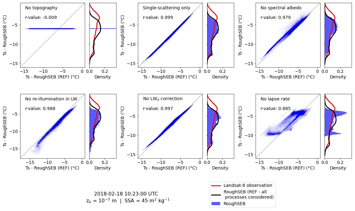
Figure 9 Impact of disabling a topographic effect on the simulated T_s on 18 February 2018. Each panel corresponds to a disabled topographic effect, with respect to the reference simulation (REF) where all the effects are included. The marginal histograms show the distribution of surface temperature for each simulation as well as the observed T_s by the satellite (red) and the reference simulation (black).

To extend these results to all the dates, Fig. 10 displays summary statistics of the difference between the simulations with a disabled topographic effect and the reference simulation. The left panel presents the mean difference between the simulation without the effect and the reference simulations (for each effect), while the standard deviation of the differences (right panel) shows how both simulations agree in terms of spatial variations. A value close to zero means that the effect is negligible in terms of average and variations, respectively.

Figure 10 Overall representation of the mean difference and standard deviation between the reference simulation (REF), where all processes are considered, and the additional simulations, where one topographic effect is disabled at a time. The whiskers of the boxplots represent the 10th and 90th percentiles of the distribution.

When no topography is taken into account (i.e. a perfectly flat surface instead of the actual topography), the snow surface temperature is uniform (−5.9 ^∘C) across the scene. This value overestimates the mean temperature of the reference simulation (−7.2 ^∘C), showing that not only the spatial variations in temperature are not represented (r value ≈0), but even on average a simulation with flat terrain is not equivalent to the mean temperature of the area with topography. This simulation highlights the considerable effect of the topography on the surface temperature and the importance to take it into account even for large-scale simulations. Considering all the 20 dates, neglecting the topography results in an overall overestimation of 1.3 ^∘C (median value), and the standard variations with respect to the reference simulation are high, with a median value of 3.2 ^∘C and a maximum of 6 ^∘C.

The simulation with single-scattering only in the SW (only the first bounce of the photons is considered by RSRT; the absorption enhancement is neglected) shows very small differences with respect to the reference simulation. It is only slightly colder, in particular in the coldest pixels. This is mainly due to neglecting the illumination in the shadowed (and cold) areas coming from slopes facing towards cold areas. Nevertheless, the impact is not significant, the mean difference being barely different from zero (median of −0.2 ^∘C, standard variations of 0.2 ^∘C). The smallest impact is observed in early winter, which could be explained by a dependence on the solar zenith angle and on how the topography modulates the received solar irradiance. Overall, this result means that, at least in our study area, the absorption enhancement caused by multiple bouncing is almost negligible.

When neglecting the spectral dependence of snow albedo and thus calculating SW_net directly from the broadband albedo (≈0.87 on 18 February 2018), the simulated surface temperature is slightly warmer than the reference, with overall differences of 0.5 ^∘C (median of the means) and of 0.7 ^∘C (median of standard deviations), with a maximum beyond 1.5 ^∘C. This shows the importance of taking into account this effect involving the coupling between spectral dependence of snow albedo and topography.

The effect of the thermal emission by surrounding terrain in the LW is obtained by estimating the surface temperature as if the terrain were flat (first step as detailed in Sect. 2.1.2). For the selected date in Fig. 9 the peak of the distribution is less marked and widened in the range of −5 to −8 ^∘C, and T_s is systematically underestimated when this approximation is applied. The difference in the warmest areas of the domain ($>-\mathrm{5}$ ^∘C) is of −0.6 ^∘C. In the coldest areas ($<-\mathrm{12}$ ^∘C), the underestimation is of −1.4 ^∘C because direct radiation is absent, and the radiation budget is dominated by diffuse and weak illumination. The thermal emission by surrounding faces warms these cold areas as a function of their sky-view factor. The mean difference is −0.7 ^∘C (standard variations of 0.6 ^∘C) when considering all the simulations.

Neglecting the altitudinal variations in the downwelling LW flux over the study area has a limited impact on T_s. Slight differences are mainly concentrated in the range of −3 to −8 ^∘C and also in the coldest areas, where the T_s is overestimated by almost 0.6 ^∘C. Parts of these zones are at the highest altitudes of the study area, and without the correction they receive more downwelling LW flux (up to ≈15–20 W m⁻²), leading to warmer surface temperature. Overall, neglecting the altitudinal variations barely overestimates the estimation of T_s by 0.2 ^∘C, with errors that are not significant (median value of 0.3 ^∘C).

With respect to the altitudinal variations in air temperature (lapse rate effect), the distribution shape squeezes and even becomes bimodal, with two marked peaks at −5 and −10 ^∘C when the lapse rate is neglected (Fig. 9). The differences to the reference simulation are significant when considering all the dates, with a median value of 0.9 ^∘C and a median standard deviation of 1.3 ^∘C. Introducing the lapse rate effect tends to warm the air in the lower parts of the domain (usually the warmest) and the opposite on the highest and coldest facets. Since the FluxAlp measurement station (where the reference air temperature is taken) is in the lower range of altitudes of the study area, the overall impact of neglecting the lapse rate effect is an overestimation (0.9 ^∘C). This result is specific to the position of the station with respect to the altitudinal distribution, and using a different reference air temperature would change this result. In contrast, the standard variations are also significant, and this is not specific to our setting. It effectively shows that neglecting the altitudinal variations in air temperature results in an overall significant error of 1.3 ^∘C (median) in surface temperature over the study area. The correlation coefficient is the lowest, with a median value of 0.921 considering all the simulations.

These results give the relative importance of the topographic effects investigated here. Neglecting the topography (i.e. assuming a flat surface) is as expected the most important source of error when simulating snow surface temperature. Neglecting the altitudinal variations in air temperature is the second effect in terms of importance. It is followed by the thermal emission by surrounding terrain in the LW and the spectral dependence of snow albedo, the latter being slightly less important. Finally, the absorption enhancement caused by multiple bouncing is almost negligible, as are the altitudinal variations in downwelling LW flux.

4 Discussion

4.1 Retrieval of surface temperature from satellite observations

The assessment of our modelling chain was performed against in situ and satellite observations, the latter being crucial for the spatial variations. However, they depend on the choice of the method for the atmospheric correction. Here we implemented two single-channel methods for Landsat 8 thermal imagery – the SC method (Jiménez-Muñoz and Sobrino, 2003) and the iSC method (Cristóbal et al., 2018) – and we compared them to the recent surface temperature product. The iSC method is the most accurate (within ≈1 ^∘C) at the FluxAlp measurement station. The Collection 2 surface temperature product is the less accurate (within 3.5 ^∘C). However, this does not preclude the quality in the whole area. In particular, we assumed that the whole scene is covered by snow, with an emissivity equal to 0.98. However, in alpine areas, vertical mountain ridges or patches without snow on sun-facing slopes are frequent and may result in a variable emissivity over the scene. A possible future improvement would be to include a land mask to set a particular emissivity value for each pixel depending on the presence of snow, rocks, grass, etc. This is normally achieved by means of normalized difference vegetation index (NDVI)-based classifications (Li et al., 2013) that can be adapted to snow-covered complex terrains with methods that rely on the snow cover area (Varade and Dikshit, 2020). The surface temperature product, which includes NDVI-based classifications, is less accurate than the methods without this refinement (at the FluxAlp station). Overall, the differences across the study area between the iSC method and this official product are 0.3 ^∘C (median of standard deviations), which is considerably lower than the difference at FluxAlp. The satellite thermal observations from Landsat 8 are therefore correct enough to assess the model performance, with an accuracy of the order of 1 ^∘C and a precision lower than 0.5 ^∘C.

4.2 Snow surface temperature estimation

The simulations show an overall agreement with both in situ measurements and satellite observations (Sect. 3.2). The simulated fluxes and the temporal evolution of T_s are well represented for a daily cycle (Fig. 6). The net SW flux is slightly underestimated during part of the day (except in the morning, when it is slightly overestimated), but the impact on surface temperature is balanced by the other terms of the energy budget. The treatment of the turbulent heat fluxes in the model at this stage is very simple: the atmosphere is assumed neutral, the aerodynamic roughness length is uniform, the wind is uniform, etc. Some of these simplifications are required for the computational performances and may be challenging to take into account, while others (e.g. atmospheric stability) could be easily implemented (Essery and Etchevers, 2004).

The ground heat flux was also neglected, which means that the surface temperature reacts immediately to changes in the downwelling radiation. In reality, the snowpack has some thermal inertia which delays and moderates the diurnal amplitude of T_s. If significant, this would lead to an overestimation in the morning and underestimation in the late afternoon, when the warming (cooling) of the surface is more pronounced in the simulations as the solar zenith angle decreases (increases). Nevertheless, this delay is barely visible in our case (Fig. 6). Snow is indeed a highly insulating material and has a small thermal inertia. Assuming a thermal conductivity of around 0.2 $\mathrm{W}{\mathrm{m}}^{-\mathrm{1}}{\mathrm{K}}^{-\mathrm{1}}$ (Sturm et al., 1997), the daily wave penetrates by no more than 20 cm into the snowpack. This means that with a diurnal cycle half-amplitude of ≈7 ^∘C in surface temperature, the maximum temperature gradient in the upper snowpack is of the order of 35 K m⁻¹. According to the Fourier law, this implies a maximum ground heat flux G≈7 W m⁻², which is an order of magnitude lower than the radiative and turbulent heat fluxes estimated in our case (Fig. 6). This simple calculation confirms that neglecting G is acceptable in a first approximation when snow is relatively fresh and is not melting. In spring, with a denser and less insulating snowpack and with melt, this approximation needs to be reconsidered. However, taking into account the thermal diffusion in the snowpack over millions of facets represents a significant computational cost.

Figure 11 Changes in simulated snow surface temperature (ΔT_s) for a diurnal cycle at the FluxAlp station when varying the specific surface area (SSA; a) and the aerodynamic roughness length (z₀; b). The shaded areas correspond to nighttime (i.e. SZA below 0^∘ or over 90^∘).

The choice of input parameters such as SSA and aerodynamic roughness length (z₀) is critical for the simulations. Local measurements are not always available and may not be representative of the whole area. SSA drives the albedo and, in turn, the short-wave absorption by the snowpack. The sensitivity of snow surface temperature to SSA is assessed in Fig. 11 (top) for the diurnal cycle presented in Fig. 6. SSA is varied by ±10 m² kg⁻¹ with respect to the reference simulation for the whole time series (20 m² kg⁻¹). The impact of varying SSA on T_s is up to 1 ^∘C and is larger when considering a low SSA than a large SSA. This is mainly due to the fact that the SSA–albedo relationship is non-linear (Domine et al., 2006). In general, spatio-temporal variations in SSA are expected in our area because the fresh-snow SSA value depends mainly on snowfall temperature, and its subsequent evolution is a general decrease depending on the thermal evolution of the snowpack (Domine et al., 2008). As a result, SSA is expected to be higher at the highest altitudes and in the shadows where the conditions are colder. Higher SSA leads to less short-wave absorption, which would tend to increase the cooling in these areas compared to lower SSA areas. The spatial variations in SSA could be modelled, for instance, using SSA retrieved by satellite (e.g. Kokhanovsky et al., 2019). The temporal variations in SSA could explain the differences between the simulated and measured SW_net flux as here the value was kept constant for the whole time series.

The aerodynamic roughness length controls the sensible and latent heat fluxes, so it shall also be carefully prescribed. In this study, a value of 10⁻³ m is assumed, which is standard according to previous works (e.g. Brock et al., 2006). The sensitivity of T_s to aerodynamic roughness length is shown in Fig. 11 (bottom); z₀ varies by a factor of 5 with respect to the reference simulation. The choice of z₀ has a significant impact on the simulated surface temperature, in particular during the night (up to 2 ^∘C), when the SW radiation is absent. Previous works (Martin and Lejeune, 1998; Kuipers Munneke et al., 2009) found similar variations with different approaches. A different formulation of the turbulent heat fluxes (e.g. atmospheric stability) could lead to smaller differences during the night, in particular with stable conditions. According to Brock et al. (2006), snow z₀ can vary by up to 3 orders of magnitude depending on the time of the season and on snow type (i.e. fresh snow or melting snow). To estimate the expected spatial variations in a mountainous area of several square kilometres, a parameterization of snow z₀ as a function of the snow type would be possible via the snow SSA (Domine et al., 2007).

The spatial variations in T_s are clearly dependent on the topography and are correctly simulated (Fig. 7). They seem to depend on slope orientation, as shown in Fig. 12. For larger slopes (>30^∘), the lack of direct radiation governs the surface temperature in some areas, such as the north-facing (north-west to north-east) shadowed slopes. The temperature difference is large between opposing slopes (on the order of 5 to 10 ^∘C). Overall, the mean T_s of the north-facing facets is −10.7 ^∘C (±1.9 ^∘C). They are considerably colder than the southern (south-east to south-west) ones (−5.6 ^∘C (±1.8 ^∘C)). These differences are consistent with previous studies (e.g. Fierz et al., 2003) and highlight the necessity of accounting for spatial variations in surface temperature in mountainous areas.

Figure 12 Distribution of simulated surface temperature as a function of the aspect for slopes larger than 30^∘. The radius of each of the 16 sectors corresponds to the normed (displayed in per cent) quantity of facets.

4.3 Role of the topographic effects

The results presented in this study show that the topography controls the surface temperature to a large extent. However modelling all the processes involved in complex terrain has prohibitive computational cost for most applications. This has an adverse outcome: some of them are usually neglected or approximated. Our modelling chain takes into account a relatively comprehensive set of effects, especially on the radiative aspects. The motivation of this study is therefore to quantify their relative importance in order to determine which ones can be neglected as a function of the targeted accuracy.

The role of the topography is quantified in Sect. 3.2.4, where we compare the reference simulation (where all effects are considered) to simulations where we disabled one effect at a time. Overall, we found that the absence of topography (i.e. terrain altitude, slope, and aspect) – and therefore the presence of variations in altitude and all kinds of shadows – is the most important effect. Errors of several degrees Celsius are to be expected if considering a flat surface. The same conclusion is drawn by Yan et al. (2016), who found significant errors in the estimation of net LW radiation flux by assuming a flat surface at a larger scale over the Tibetan Plateau.

Yan et al. (2016) also accounted for the sky-view factor and the contribution of thermal radiation coming from surrounding terrain. Our results show a cooling effect of almost 1 ^∘C (median of −0.7 ^∘C) when disabling these two topographic effects. This agrees with the results presented by Arnold et al. (2006), showing a similar ratio of importance between the shadows and the LW contribution when considering glacier melt. To take this effect into account, the downwelling LW radiation flux in each facet is updated with the thermal emission of the surrounding facets, which is derived from an average T_s over the whole scene. Such an approximation saves a lot of computation time, but, as a result, the differences in thermal emission due to spatial variations in surface temperature are masked. In reality, the warmest facets emit more LW radiation than the coldest ones, leading to spatial differences in the T_s. Neglecting the variations in altitude of the downwelling LW flux has a lower influence on surface temperature. For the selected simulation (Fig. 9), the elevation-corrected flux spans from 180 to 213 W m⁻², while the measured flux is 204 W m⁻². This range is consistent with other works (Greuell et al., 1997; Iziomon et al., 2003), and the impact on T_s is only significant (>0.5 ^∘C) in the coldest areas.

Our results show a significant impact on the simulated T_s when disabling the altitudinal variations in air temperature, with a warming effect up to 1 ^∘C. The spatial and temporal distribution of air temperature, as well as wind dynamics in mountainous areas, has been widely investigated (Jiménez and Dudhia, 2012; Rotach et al., 2015). Different parameterization and estimation methods exist to overcome their complexity (e.g. Wood et al., 2001). The approach implemented here is simple, with several approximations and rough assumptions (as a constant aerodynamic roughness length and wind speed across the study area). Future improvements of our approach could benefit from wind downscaling methods to better represent wind speed distribution over complex terrain, as in Helbig et al. (2017).

This study accounts for the spectral dependence of snow albedo, which is an improvement with respect to most of the models that only account for broadband albedo. As running RSRT at many wavelengths is very expensive, we developed the effective method present in Eqs. (5) and (6). The impact on T_s is limited, but errors up to ≈1.5 ^∘C are possible. The relative importance is similar to that of the thermal emission from surrounding slopes and is not negligible.

The last topographic effect investigated here is the influence of the multiple bounces of photons between the faces in the short-wave domain, also called re-illumination or cause of absorption enhancement. It is simulated with the RSRT model (Larue et al., 2020) and represents the most expensive step of the modelling chain in terms of computational cost as each photon is tracked until it escapes the scene, after one or several bounces. The results presented here suggest that the re-illumination can be neglected, with a limited impact on the surface temperature estimations (<0.2 ^∘C). This implies that RSRT is only needed to track the shadows and slope and compute the sky-view factor. In principle these effects can be taken into account by other faster methods (e.g. Dozier et al., 1981). Nevertheless, other authors have drawn different conclusions regarding the role of re-illumination in the same study area. Lamare et al. (2020) found a significant contribution of multiple reflections on the simulated top-of-atmosphere (TOA) radiance in the same area as ours. A hypothesis to explain this discrepancy is the dependence on the sun's position and the configuration of the terrain. Earlier simulations in the winter season (closer to 1 December) show a lower impact than later ones. However, this point requires further investigation, in particular as atmospheric scattering and absorption effects due to the air within the relief are neglected in the present work.

5 Conclusions

We have investigated the relative importance of several topographic effects in a mountainous terrain in the French Alps. For this, we have first developed a modelling chain to predict surface temperature, combining existing radiative transfer models (RSRT, SBDART) and a new surface energy budget model (RoughSEB). This chain was evaluated against in situ measurements and remote sensing thermal observations to account for the spatial variations.

A ≈36 h long time series was simulated, and an overall agreement is achieved with the in situ measurements, within 0.2 ^∘C. Besides, the bias of the simulations at the FluxAlp station for the 20 scenes corresponding to the Landsat 8 acquisitions is only −0.2 ^∘C (total error of 1.2 ^∘C RMS), which highlights the potential of the chain to simulate surface temperature within a reasonable accuracy and precision. The spatial variations across the 50 km² scene are also well represented, with differences to the satellite observations mainly comprised between 1 and 3 ^∘C, which is small compared to the actual surface temperature variations of 5–10 ^∘C between the slopes in the study area.

The topographic effects responsible for such spatio-temporal variations are ranked by order of importance: (1) the modulation of solar irradiance by the terrain slope and aspect (i.e. the presence of topography), (2) the altitudinal changes in air temperature (lapse rate effect), (3) the contribution of thermal radiation coming from surrounding terrain, (4) the spectral dependence of snow albedo, (5) the changes in downward long-wave flux because of variations in altitude, and (6) the absorption enhancement caused by multiple bouncing of photons in the SW domain.

A future possible extension of the modelling chain should aim at investigating snowmelt and patchy snow conditions. An application is the preparation of the thermal infrared TRISHNA satellite mission (Lagouarde et al., 2019) and in the future its calibration and validation. From 2025, TRISHNA will provide high-resolution images (50 m) of the Earth surface temperature in mountainous areas with a 3 d revisit time.

Appendix A: Additional equations and mathematical developments

A1 Snow spectral albedo in the asymptotic radiative transfer (ART) theory

The direct and diffuse components of the snow spectral albedo are computed using the ART theory (Kokhanovsky and Zege, 2004). We assume that the snowpack is semi-infinite, and the surface is flat and smooth (the facets of the mesh are small enough to be considered smooth surfaces). The albedos are expressed as follows:

$$\begin{array}{}\text{(A1)}& {\displaystyle }{\mathit{\alpha }}_{\text{dir}}(\mathit{\lambda },{\mathit{\theta }}_{\text{s}})=\exp \left(-{\displaystyle \frac{\mathrm{12}(\mathrm{1}+\mathrm{2}\cos {\mathit{\theta }}_{\text{s}})}{\mathrm{7}}}\sqrt{{\displaystyle \frac{\mathrm{2}B\mathit{\gamma }\left(\mathit{\lambda }\right)}{\mathrm{3}{\mathit{\rho }}_{\text{ice}}\text{SSA}(\mathrm{1}-g)}}}\right)\text{(A2)}& {\displaystyle }{\mathit{\alpha }}_{\text{diff}}\left(\mathit{\lambda }\right)=\exp \left(-\mathrm{4}{\displaystyle \frac{\sqrt{\mathrm{2}B\mathit{\gamma }\left(\mathit{\lambda }\right)}}{\mathrm{3}{\mathit{\rho }}_{\text{ice}}\text{SSA}(\mathrm{1}-g)}}\right),\end{array}$$

where θ_s is the solar zenith angle, SSA is the snow specific surface area, ρ_ice=917 kg m⁻³ is the bulk density of ice at 0 ^∘C, γ(λ) is the ice absorption coefficient (Picard et al., 2016), and B and g are the shape coefficients of snow (Libois et al., 2014).

A2 Surface exchange coefficient

The surface exchange coefficient involved in the calculation of the turbulent heat fluxes is given by

$$\begin{array}{}\text{(A3)}& C_{\text{H}}=\mathrm{0.16}{\left[\ln \left({\displaystyle \frac{z_{\text{t}}}{z_{\mathrm{0}}}}\right)\ln \left({\displaystyle \frac{z_{\text{w}}}{z_{\mathrm{0}}}}\right)\right]}^{-\mathrm{1}},\end{array}$$

where z_t and z_w are the heights at which air temperature and wind speed are measured, respectively, and z₀ is the aerodynamic roughness length. Their values are provided in Table B1.

A3 General solution of the quartic equation

The simplified surface energy budget equation Eq. (14) eventually becomes a quartic equation, with T_s as the unknown:

$$\begin{array}{}\text{(A4)}& a{T}_{\text{s}}^{\mathrm{4}}+d{T}_{\text{s}}+e=\mathrm{0},\end{array}$$

where a, d, and e are constant for each facet. The general solution of this equation requires a simple change of variable to transform the quartic into a depressed quartic:

$$\begin{array}{}\text{(A5)}& T_{\text{s}}^{\mathrm{4}}+p{T}_{\text{s}}^{\mathrm{2}}+q{T}_{\text{s}}+r=\mathrm{0},\end{array}$$

which can be solved by means of the Ferrari solution (Neumark, 1965). It consists of adapting the equation to present it as a difference of two squares, which eventually leads to a resolvent cubic that is then solved, yielding

$$\begin{array}{}\text{(A6)}& {\displaystyle }{T}_{\text{s}}{\displaystyle }=-S+{\displaystyle \frac{\mathrm{1}}{\mathrm{2}}}\sqrt{-\mathrm{4}{S}^{\mathrm{2}}+{\displaystyle \frac{q}{S}}},\end{array}$$

where q is the simplified first-degree coefficient of the depressed quartic equation ($q=d/a$) and where

$$\begin{array}{}\text{(A7)}& {\displaystyle }S& {\displaystyle }={\displaystyle \frac{\mathrm{1}}{\mathrm{2}}}\sqrt{{\displaystyle \frac{\mathrm{1}}{\mathrm{3}a}}\left(Q+{\displaystyle \frac{{\mathrm{\Delta }}_{\mathrm{0}}}{Q}}\right)}\text{(A8)}& {\displaystyle }Q& {\displaystyle }=\sqrt[\mathrm{3}]{{\displaystyle \frac{{\mathrm{\Delta }}_{\mathrm{1}}+\sqrt{{\mathrm{\Delta }}_{\mathrm{1}}^{\mathrm{2}}-\mathrm{4}{\mathrm{\Delta }}_{\mathrm{0}}^{\mathrm{3}}}}{\mathrm{2}}}},\end{array}$$

with

$$\begin{array}{}\text{(A9)}& {\displaystyle }{\mathrm{\Delta }}_{\mathrm{0}}& {\displaystyle }=\mathrm{12}ae\text{(A10)}& {\displaystyle }{\mathrm{\Delta }}_{\mathrm{1}}& {\displaystyle }=\mathrm{27}a{d}^{\mathrm{2}}.\end{array}$$

A4 Land surface temperature retrieval from Landsat 8

LST is calculated for each pixel by applying the radiative transfer equation to a sensor channel (Eqs. 1 to 3 in Cristóbal et al., 2018), which leads to

$$\begin{array}{}\text{(A11)}& \text{LST}=\mathit{\gamma }\cdot \left[{\mathit{\epsilon }}^{-\mathrm{1}}({\mathit{\psi }}_{\mathrm{1}}\cdot L_{\text{sensor},\mathit{\lambda }}+{\mathit{\psi }}_{\mathrm{2}})+{\mathit{\psi }}_{\mathrm{3}}\right]+\mathit{\delta },\end{array}$$

where

$$\begin{array}{}\text{(A12)}& {\displaystyle }& {\displaystyle }\mathit{\gamma }={\left\{{\displaystyle \frac{c_{\mathrm{2}}\cdot L_{\text{sensor},\mathit{\lambda }}}{T_{\text{sensor}}^{\mathrm{2}}}}\left[{\displaystyle \frac{{\mathit{\lambda }}^{\mathrm{4}}}{c_{\mathrm{1}}}}{L}_{\text{sensor},\mathit{\lambda }}+{\mathit{\lambda }}^{-\mathrm{1}}\right]\right\}}^{-\mathrm{1}}\text{(A13)}& {\displaystyle }& {\displaystyle }\mathit{\delta }=-\mathit{\gamma }\cdot L_{\text{sensor},\mathit{\lambda }}+T_{\text{sensor}}\text{(A14)}& {\displaystyle }& {\displaystyle }{T}_{\text{sensor}}={\displaystyle \frac{K_{\mathrm{2}}}{\ln \left(\frac{K_{\mathrm{1}}}{L_{\mathit{\lambda }}}+\mathrm{1}\right)}},\end{array}$$

where ε is the emissivity of the pixel, ψ_i represents the atmospheric functions that are parameterized, λ is the effective wavelength (10.904 µm for Band 10), L_sensor,λ is the top-of-atmosphere radiance calculated from pixel digital numbers (DNs) using rescaling factors (USGS, 2021), and T_sensor is the brightness temperature in kelvin. Values of the symbols can be found in Table B1.

The atmospheric functions are statistically fitted from the GAPRI database (Mattar et al., 2015) containing 4714 atmospheric profiles from tropical to arctic atmospheric conditions. The following fit is applied here:

$$\begin{array}{}\text{(A15)}& \begin{array}{rl}{\mathit{\psi }}_i& =i{w}^{\mathrm{2}}+h{T}_{\text{a}}^{\mathrm{2}}+gw+f{T}_{\text{a}}+e{T}_{\text{a}}^{\mathrm{2}}w+d{T}_{\text{a}}w\\ & +c{T}_{\text{a}}{w}^{\mathrm{2}}+b{T}_{\text{a}}^{\mathrm{2}}{w}^{\mathrm{2}}+a.\end{array}\end{array}$$

All the coefficient values (from i to a) are in Cristóbal et al. (2018).

Appendix B: Table of symbols

Table B1 Definitions and values of the symbols and magnitudes that appear in this paper.

Appendix C: List of selected Landsat 8 scenes

Table C1 List of selected scenes.