the Creative Commons Attribution 4.0 License.
the Creative Commons Attribution 4.0 License.
 | 02 Dec 2022
Stochastic analysis of micro-cone penetration tests in snow
Isabel Peinke
Pascal Hagenmuller
Matthias Wächter
M. Reza Rahimi Tabar
Joachim Peinke
Cone penetration tests have long been used to characterize snowpack stratigraphy. With the development of sophisticated digital penetrometers such as the SnowMicroPen, vertical profiles of snow hardness can now be measured at a spatial resolution of a few micrometers. By using small penetrometer tips at this high vertical resolution, further details of the penetration process are resolved, leading to many more stochastic signals. An accurate interpretation of these signals regarding snow characteristics requires advanced data analysis. Here, the failure of ice connections and the pushing aside of separated snow grains during cone penetration lead to a combination of (a) diffusive noise, as in Brownian motion, and (b) jumpy noise, as proposed by previous dedicated inversion methods. The determination of the Kramers–Moyal coefficients enables differentiating between diffusive and jumpy behaviors and determining the functional resistance dependencies of these stochastic contributions. We show how different snow types can be characterized by this combination of highly resolved measurements and data analysis methods. In particular, we show that denser snow structures exhibited a more collective diffusive behavior supposedly related to the pushing aside of separated snow grains. On less dense structures with larger pore space, the measured hardness profile appeared to be characterized by stronger jump noise, which we interpret as related to breaking of a single cohesive bond. The proposed methodology provides new insights into the characterization of the snowpack stratigraphy with micro-cone penetration tests.
- Article
(3352 KB) - Full-text XML
- BibTeX
- EndNote


Snow is an essential component of our environment and can significantly impact our lives: from the wishful dream of a white Christmas to the misfortune of avalanche accidents. Having a closer look at snow, one discovers many microstructural patterns and realizes that snow on the ground undergoes constant evolution (Colbeck et al., 1990). The snow microstructure fully controls its physical and mechanical properties, which are essential for diverse applications, such as avalanche forecasting (Schweizer et al., 2003). A snowpack is typically structured in numerous layers composed of different snow types, where such stratigraphy will determine the snowpack stability. Cone penetration tests have long been used to characterize the snowpack stratigraphy (Bader and Niggli, 1939). The SnowMicroPen (SMP) can perform cone penetration tests of snow in the field (Schneebeli et al., 1999). It measures the force needed to drive a cylinder with a millimetric conic tip into the snowpack. With its high resolution (250 measurements mm−1), the measured force or hardness is supposedly linked to the snow microstructure (Johnson and Schneebeli, 1999). A typical consequence of such a high-precision measurement is that more and more details of the penetration process can be resolved, leading to many more stochastic signals. In this context, it is of particular interest to employ advanced data analysis to find out how different kinds of stochastic signals are related to different snow types. There are also other penetrometers used for cone penetration tests in the field of snow; for example McCallum (2013) used a large-scale penetrometer with a tip diameter of 36.7 mm in polar snow. For our analysis, we specifically used the measurement data of micro-cone penetration tests from Schneebeli et al. (1999).
Johnson and Schneebeli (1999) developed the first model to estimate micromechanical properties of snow from measured penetration profiles. They assumed that the material compaction is negligible and that the penetration resistance is only composed of friction between the penetrometer and snow grains and a superposition of spatially uncorrelated and identical brittle failures of individual snow microstructural elements (e.g., the bonds between the snow grains). Marshall and Johnson (2009) extended the theory of Johnson and Schneebeli (1999) to account for simultaneous ruptures by Monte Carlo simulations. They precisely resolved the snow micromechanical parameters, such as the deflection length, rupture force and rupture intensity. Löwe and van Herwijnen (2012) re-stated the pioneering idea of Johnson and Schneebeli (1999) and described the fluctuating penetration hardness as a Poisson shot noise process. In their model, the micromechanical parameters can be simply derived from the cumulants and the co-variance of the penetration signal. Peinke et al. (2019) further extended the homogeneous Poisson process of Löwe and van Herwijnen (2012) so that the scale of variation in the rupture intensity could be decoupled from the scale of variations in the deflection length and the rupture force. These models are now commonly used to characterize the snowpack stratigraphy from SMP measurements. Indeed, Proksch et al. (2015) related the micromechanical parameters derived from SMP measurements to some of the most critical snow characteristics, namely density, specific surface area and structural correlation length. These relations are now routinely used to quantify the snowpack stratigraphy (e.g., Calonne et al., 2020). Besides, Reuter et al. (2019) estimated the elastic modulus and fracture energy from the micromechanical parameters, which can then be used to compute point snow stability for avalanche hazard assessment (e.g., Reuter et al., 2015).
Here, we consider the measured fluctuating hardness as a consequence of summing up the interactions between the penetrometer tip and individual snow particles. We describe this penetration process in analogy to the well-known Brownian motion (Einstein, 1905), where a microscopically visible particle suspended in fluid is moving randomly. Due to the sum of several collisions with the molecules in the fluid as illustrated in Fig. 1, the large red particle undergoes a motion described by a stochastic process. Such a stochastic process is driven by white noise and is known as a Langevin process (see Gardiner, 1985, and Sect. 2). While very similar elementary collision events are assumed for classical Brownian motion, we also need to consider brittle failures of individual snow microstructural elements (bonds between snow grains, crushing of grain clusters), which cause sharp declines in penetration hardness. These brittle failures were modeled as a Poisson shot noise process by Löwe and van Herwijnen (2012) and Peinke et al. (2019). Jump noise acts as discontinuous paths inside the diffusion process, and low-jump events can be considered Poisson distributed noise (which corresponds to the abovementioned shot noise). The idea of this work is to employ a method that allows estimating the underlying stochastic differential equation from empirical data and differentiating between a Langevin (pure diffusive) and a jump-diffusion process (Anvari et al., 2016). Via this advanced analysis, we seek more detailed snow characterization from micro-cone penetration test resistance data.1
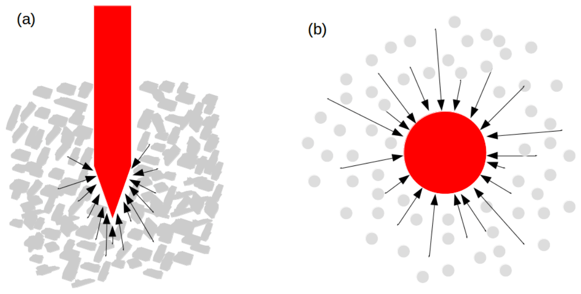
Figure 1(a) Penetration resistance caused by the interactions of the snow particles (gray) with the penetrometer tip (red); (b) Brownian motion where a microscopically visible particle (red) suspended in the fluid is moving randomly due to the collisions with the molecules (gray) in the fluid.
The article is organized as follows. In Sect. 2, we summarize the stochastic analysis method and show how it is possible to distinguish between diffusive and jump noise. In Sect. 3, the method is applied to centimetric snow samples whose microstructure is also captured by tomography. In Sect. 4, as a proof of concept, the SMP profile of a natural snowpack is analyzed with this technique.
A stochastic process x(t) can be described through stochastic differential equations. This section explains the equations used to model cone penetration tests in snow. Since the SMP is driven by a motor with constant speed (z is depth; t is time) and samples the measurement every 4 µm, the measured penetration force or snow hardness R is considered the depth dynamics R(z(t)) and handled like a stochastic variable x(t).
2.1 Langevin equation
A diffusive process x(t), which is a continuous stochastic process, follows the Langevin equation, where for a small step size dt has the following expression (Risken, 1984; Friedrich et al., 2011; Tabar, 2019):
where D(1)(x,t) and D(2)(x,t) are the drift and the diffusion coefficients, respectively, and Wt is the Wiener process. The drift term D(1) describes how fluctuations relax to the local mean values of x, defined by . The diffusion term D(2) represents the amplitude of the noise. The coefficients D(1) and D(2) are also known as the first- and second-order Kramers–Moyal (KM) coefficients, respectively. In general, KM coefficients can be directly determined from the given data x(t) using their definitions of the conditional incremental average (Friedrich et al., 2011; Tabar, 2019); i.e.,
Further details on methods of this estimation can be found in Friedrich et al. (2011) and Rinn et al. (2016)2. The Langevin equation describes a continuous diffusion process where for j≥3 and . According to Pawula's theorem, all KM coefficients K(j) are vanishing for j≥3 if (Risken, 1984; Pawula, 1967). In our case, however, the higher-order coefficients are not always vanishing; hence we extend the discussion to the jump-diffusion process (see Sect. 2.2).
For the SMP data considered, the drift term D(1) in Eq. (1) describes how hardness fluctuations relax to the local mean values of hardness R, defined by . The diffusion D(2) term represents the amplitude of the hardness fluctuations. The coefficients D(1) and D(2) are z-dependent for non-stationary (inhomogeneous) processes. Here, we assume that for a chosen small depth interval (z), D(1)(R,z) and D(2)(R,z) only depend on R (similarly to Löwe and van Herwijnen, 2012, for their shot noise model).
2.2 Jump-diffusion dynamics
Typically, when the signal of a stochastic process presents sharp changes at some instant (discontinuity events), higher-order Kramers–Moyal coefficients (especially K(4)(x,t)) become non-negligible. In this case, an extension to Langevin-type modeling with additional jump noise is needed (see Tankov, 2003; Stanton, 1997; Johannes, 2004; Bandi and Nguyen, 2003; Anvari et al., 2016; Tabar, 2019). Such a jump-diffusion dynamic is given by the following stochastic differential equation:
where, again, D(1) and D(2) are the drift and the diffusion coefficients, respectively, and Wt is the Wiener process. The quantity ξ is the size of the jump noise and is assumed to be normally distributed; i.e., , where is the so-called jump amplitude. The term Jt is the Poisson jump process, which is the zero–one jump process with a jump rate (or intensity) λ(x,t) (Hanson, 2007; Tabar, 2019).
For jump-diffusion processes, the drift and diffusion coefficients (D(1), D(2)), the jump rate and amplitude λ are related to the KM coefficients as (Anvari et al., 2016):
The estimate of the drift coefficient is the same for the diffusion process (Eq. 1) and the jump-diffusion process (Eq. 4). Jump amplitude and rate λ can be estimated by using Eq. (6) with j=4 and j=6 and Wick's theorem (Isserlis, 1916; Wick, 1950) for Gaussian random variables, which states that :
To improve the estimation of KM coefficients K(j)(x,t) and in particular of high-order coefficients, the Nadaraya–Watson estimator, which is a kernel estimator, can be used (Nadaraya, 1964; Watson, 1964):
where here we use a Gaussian kernel k(u) (Tabar, 2019). With the kernel-based method the conditional moments can be calculated more smoothly by controlling the kernel bandwidth h (Lamouroux and Lehnertz, 2009), where here we use the kernel bandwidth h=0.3.
For the SMP measurements considered, we also assume that for a chosen small depth interval (z), D(1)(R,z), D(2)(R,z), and λ(R,z) only depend on R. The stochastic differential equation for the jump-diffusion process thus reads, at small depth intervals, as
with an interpretation of the drift and diffusion terms (D(1), D(2)) analogous to the purely diffusive process (Eq. 1) but now extended by a jump noise term. This is the same as Eq. (3) in terms of depth z instead of time t. The jump rate λ has the dimension of and can be related to the shot noise intensity described by Löwe and van Herwijnen (2012) and Peinke et al. (2019). Typically, λ dz corresponds to the stochastic average of the number of jumps for a penetration increment of depth dz (Anvari et al., 2016; Tabar, 2019). The jump amplitude represents the square of the typical size of a jump. Note that the jump can be negative (failure of a microstructural element) or positive (loading of a microstructural element). Here, we do not consider any progressive loading of a microstructural element as described by Löwe and van Herwijnen (2012) and Peinke et al. (2019) with the microstructural deflection length δ. Here, the loading of a microstructural element and its contribution to penetration hardness are considered instantaneous.
2.3 Synthetic examples
In this section, we illustrate how diffusive and jump noises affect the stochastic fluctuations on a synthetic example. An Ornstein–Uhlenbeck (OU) process x is described by a stochastic differential equation (SDE) with linear relaxation dynamics and an additive uncorrelated noise. With an additional jump term, it is defined as
where γ is the relaxation rate, D the constant diffusion coefficient and Wt a scalar Wiener process. The noise is assumed to be normally distributed with the constant variance or jump amplitude . Jt∼P(λt) is the Poisson jump process, which is a zero–one jump process with constant jump rate λ. Here, we have triply stochastic processes Wt, Jt and ξ, which are assumed to be independent of each other.
Three synthetic time series of the OU jump-diffusion process were generated for with , and for the additional jump terms with and . The generated data were normalized with their respective standard deviation. In Fig. 2 the normalized time series of the OU jump-diffusion processes are shown. A pure diffusion process (left), a drift-jump process (middle) and the combined jump-diffusion process (right) are shown. The fourth-order KM coefficients K(4)(x) of each time series are also plotted in Fig. 2, bottom row. K(4) of the diffusion process is negligibly small compared to drift-jump and jump-diffusion processes.
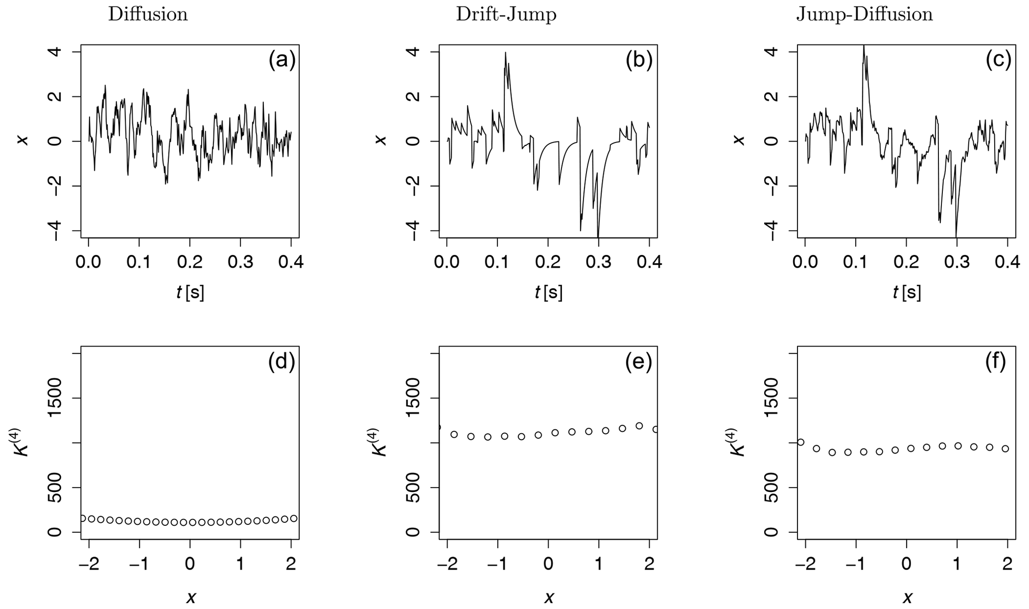
Figure 2Normalized time series of Ornstein–Uhlenbeck processes with only diffusion, only jump (drift-jump) and jump-diffusion terms (a, b, c) and their fourth-order KM coefficients K(4) (d, e, f). K(4) of the diffusion process is negligible compared to drift-jump and jump-diffusion processes. For all three examples, we used the same noises in the stochastic part of the stochastic differential equation.
For a jump-diffusion process, another parameter that we considered was the ratio of diffusion and jump noise , which becomes here for our OU jump-diffusion process . To validate our method, based on the KM coefficients of Eq. (5) to Eq. (8), three pairs of parameters were chosen: (i) , ; (ii) , ; and (iii) , . The other parameters are the same as in the previous example. The normalized time series of these examples are plotted in Fig. 3, top row. In Fig. 3, bottom row, the ratios of diffusion and jump noise estimated from each time series were compared to the expected values (blue lines). As we used normalization and the same noises in simulation, all time series are very similar; however, one can observe clearly the much noisier fine structure in case (iii) where the diffusion coefficient is larger.
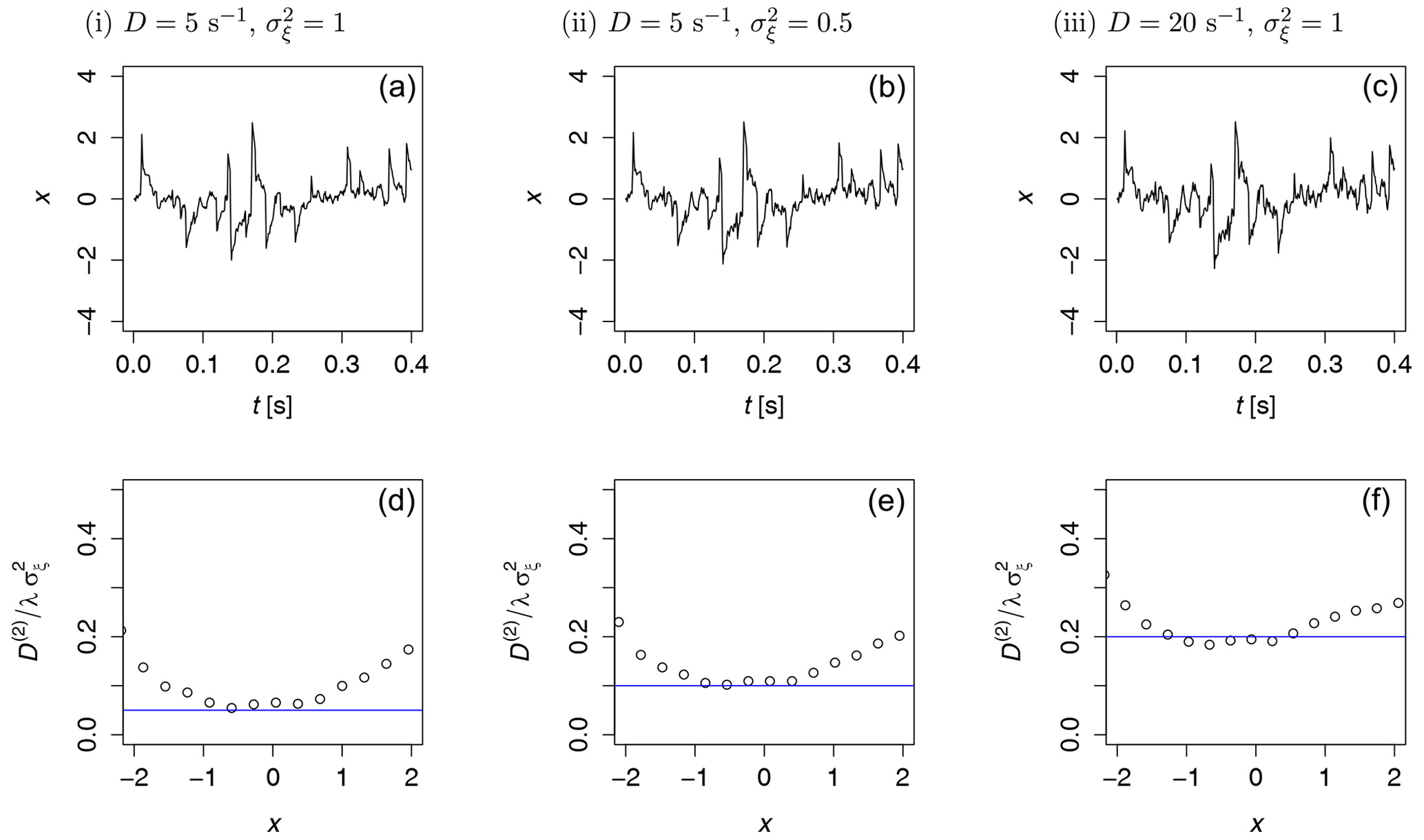
Figure 3Normalized time series of OU jump-diffusion processes with , and for (i) , ; (ii) , ; and (iii) , (a, b, c) and the corresponding ratio of diffusion and jump noise (d, e, f). Dots are results from the KM coefficients, and the blue line denotes the theoretical values given by the constants. For all three examples, we used the same noises in the stochastic part of the SDE.
In this section, our main aim is to show how the jump-diffusion model can be used to distinguish snow types from hardness profiles measured with the SMP. Firstly, small snow samples whose microstructure was also fully characterized by tomography before being measured by the SMP were used to test the developed methodology. Secondly, as a proof of concept, we analyzed one penetration profile of a snowpack measured in the field and we provided the subsequent profile of microstructural parameters. Last, the results were discussed.

Figure 4Three-dimensional view of the microstructure of some representative samples: precipitation particles (PP1), depth hoar (DH1), rounded grains (RG1) and large rounded grains (RGlr1). The ice matrix is shown in gray; the pore space is transparent. Sub-samples shown are cubic with a side length of 3 mm. Details on the data acquisition can be found in Peinke et al. (2020).
3.1 Laboratory samples
3.1.1 Measurement data
We tested several snow samples composed of four different natural snow types, namely precipitation particles (PP), depth hoar (DH), rounded grains (RG) and large rounded grains (RGlr) as classified in Fierz et al. (2009). The samples were prepared by sieving snow into small sample holders (diameter and height of 20 mm) and letting them sinter for a couple of days at −10 ∘C. Their microstructure was captured with X-ray tomography at a nominal resolution of 15 µm (Fig. 4). The cone penetration test was conducted with a modified version of the SMP, as shown in Fig. 5. More information on sample preparation and the SMP measurement can be found in the study of Peinke et al. (2020). The main sample properties are summarized in Table 1, and the measured hardness profiles (one example for each snow type) are plotted in Fig. 6. The first 4 mm is affected by the progressive penetration of the conic tip and was not considered in the stochastic analysis (Peinke et al., 2019). The remaining profiles were divided into smaller segments of a depth of 10 mm.
Table 1Overview of the detailed properties of the snow samples used. Snow types are classified according to the international classification of snow on the ground (Fierz et al., 2009). The density and specific surface area (SSA) are derived from the tomographic images from Peinke et al. (2020). Additionally, the standard deviations σR of the detrended profiles are calculated.
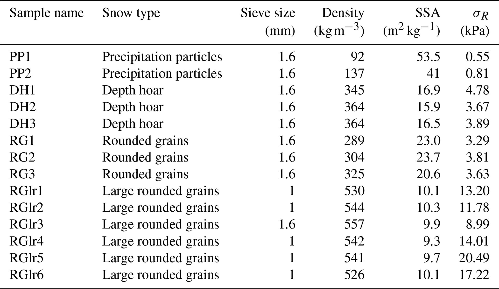
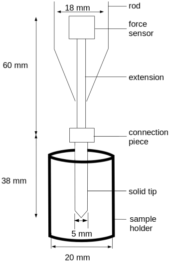
Figure 5Setup of micro-cone penetration test (Peinke et al., 2020). The cone penetration tests (CPTs) were conducted by inserting a cylinder of diameter 5 mm, with a conical tip of an apex angle of 60∘, into the snow samples. The samples were placed in the cylinder sample holder with a diameter of 20 mm. The cone was inserted vertically at a constant speed of 20 mm s−1. The SMP force sensor (Kistler 9207) measures forces in the range of [0, 40] N with a resolution of 0.01 N.
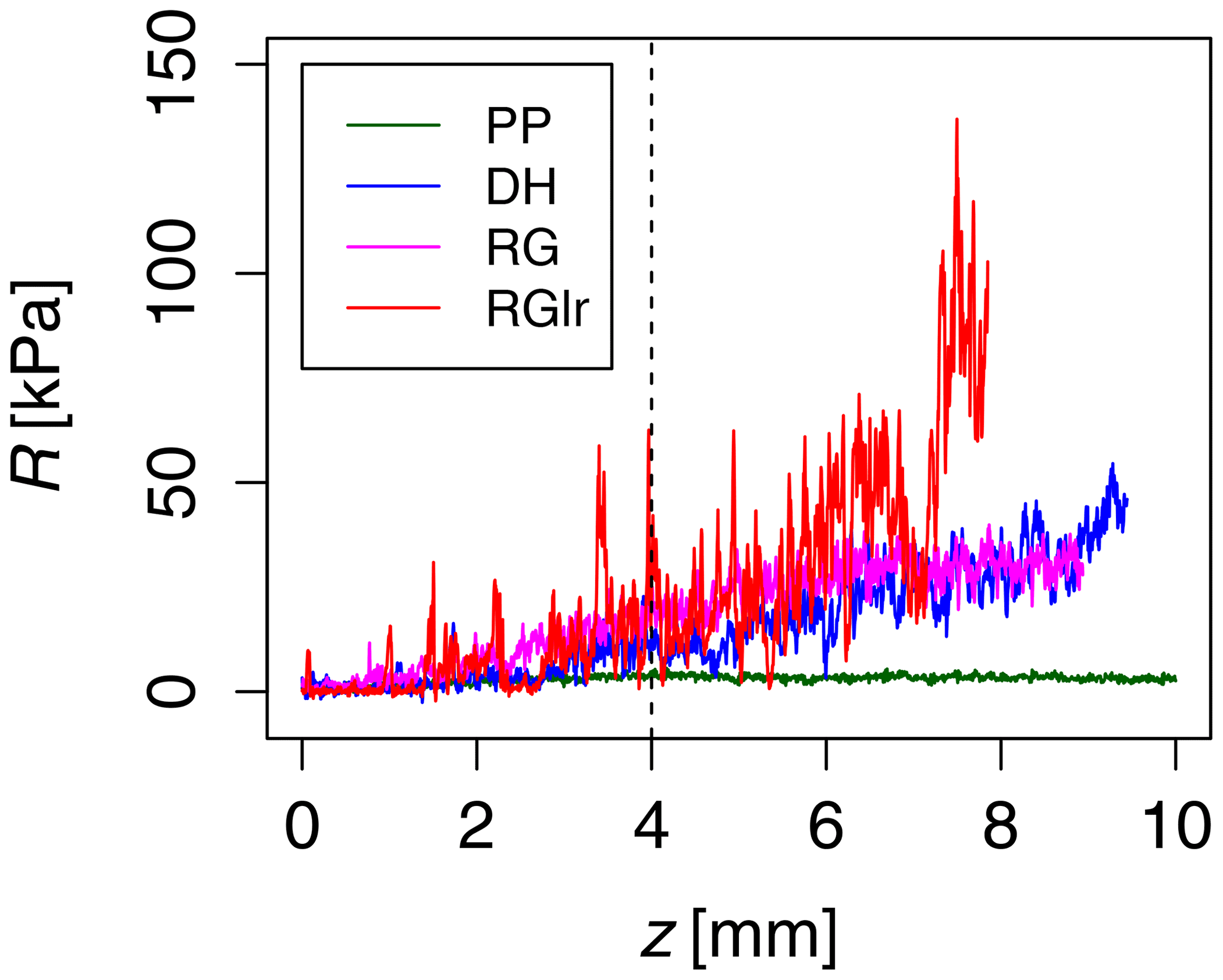
Figure 6Segments of snow hardness profiles of PP1, DH1, RG1 and RGlr1. These four different types occur as natural snow types. Precipitation particles (PP) have the smallest trend and fluctuation force; large rounded grains (RGlr) are the largest, while depth hoar (DH) and rounded grains (RG) have similar trends and fluctuation forces between those of PP and RGlr. The first 4 mm is affected by the progressive penetration of the conic tip and was not considered in the stochastic analysis.
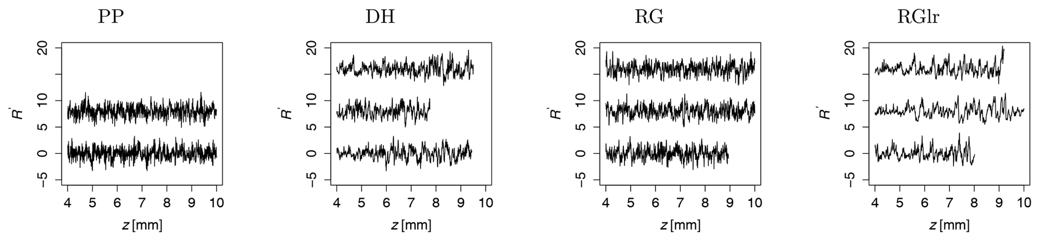
To work out the significance of advanced stochastic features for snow, we focused on the fluctuations in the hardness profiles. Each profile was first detrended. The trend was computed as the convolution of the original signal with a Gaussian kernel with a standard deviation of 0.6 mm.3 The fluctuation amplitude σR was computed as the standard deviation of . The detrended profiles are defined as . The detrended profiles R′ are characterized by a zero mean and a standard deviation of 1. The average value of on the segment and the value of the standard deviation σR are shown for each segment in Table 1. The detrended profiles R′ are shown in Fig. 7, for all four snow types.
To estimate errors, we divided the detrended and normalized data into different sub-samples. Given are two PP, three DH, three RG and six RGlr measurement profiles. These profiles were separated into smaller segments, which finally gives four PP, five DH, five RG and six RGlr samples. We estimated the KM coefficients of each sample using Eq. (2) and averaged them over the sub-samples of each snow type. Thus, drift, diffusion functions and jump parameters and their errors were estimated. The errors were reported as the standard error of the means.
3.1.2 Results
According to the description provided in Sect. 2, the drift D(1)(R′) and diffusion D(2)(R′), as well as the fourth-order KM coefficients K(4)(R′), for normalized data were determined for the four different snow types, PP, DH, RG and RGlr as shown in Fig. 8. In addition, the autocorrelation function (ACF) was determined from the signals. If the fluctuations in R′(z) belong to the diffusion processes, one would expect that . However, we find that in general, and the higher-order KM coefficients are not negligible. This indicates the presence of discontinuities in the snow hardness profile, so the jump-diffusion model is considered. Therefore, we estimated jump parameters, i.e., jump amplitudes and jump rates λ(R′) from data of R′(z) in Fig. 9.

Figure 8State-dependent drift D(1)(R′), diffusion D(2)(R′), fourth-order KM coefficients K(4)(R′) and their respective autocorrelation functions (ACFs) of four different snow types, PP, DH, RG and RGlr (left to right). The errors are shown as gray-shaded background. The red lines in the ACF plots indicate the correlation length scales determined from ACFs. Comparing the correlation length scales where with those of the autocorrelation functions (ACFs), we find that both length scales have the same ordering of their values for all snow types.
As shown in Fig. 8, the drift coefficients, , are mostly linear functions with negative slopes, which describe how fast the system tends back toward the stable fixed point. Due to our normalization, the fixed point of dynamics is located at the origin, i.e., . Taking , the correlation length scale is given by . For each snow type, LC was determined for : . Comparing LC with the correlation lengths of the autocorrelation functions – LACF, – we find that both length scales have the same ordering of their values for all snow types. The snow types PP and RG have the shorter correlation length scale, in comparison to the snow types DH and RGlr.
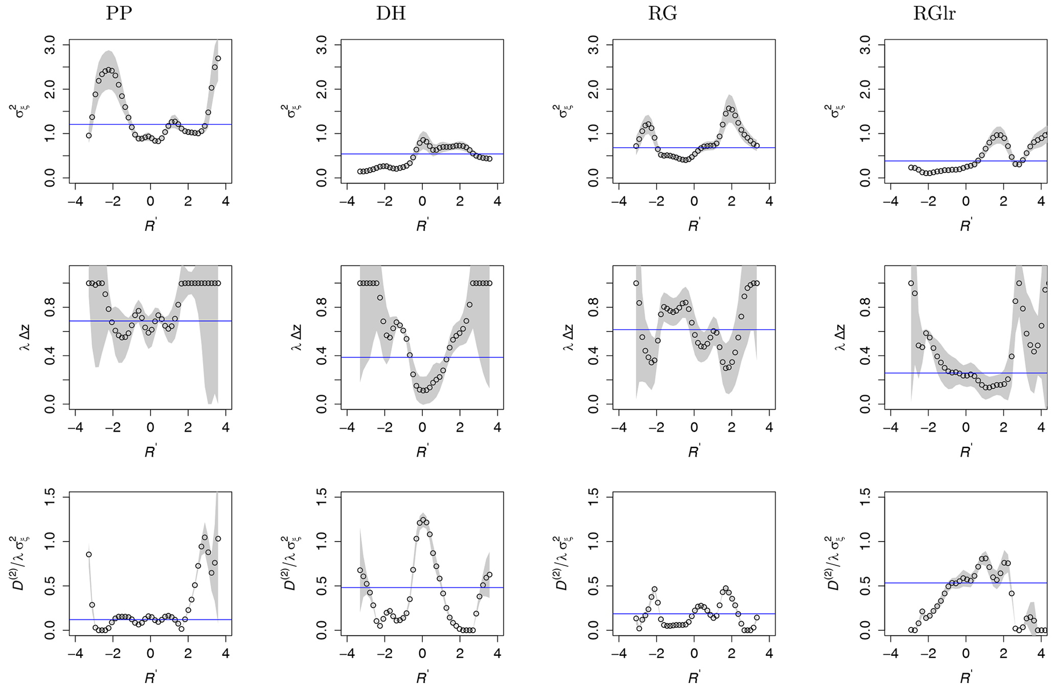
Figure 9Jump amplitudes , jump probabilities λ(R′) Δz, and diffusion and jump ratios of four different snow types, PP, DH, RG and RGlr (left to right). More data are present in the range of ; we focus our statistical analysis in this range with fewer uncertainties. The errors are shown as gray-shaded background. The ratios of diffusion and jump noise for PP and RG are minimum near zero and maximum for DH and RGlr, which means that the larger the ice structure, the stronger the diffusion noise, and vice versa. The horizontal blue lines show the mean values of the respective parameters in the range of .
The jump amplitudes, , and the jump probabilities, λ(R′) Δz, are shown in Fig. 9. The jump amplitude, , indicates how large the jump noise for different R′ values is. The jump probability describes how probable jumps or discontinuities in forces can occur. To analyze whether diffusion or jump noise is dominating, the dimensionless ratio of diffusion and jump noise (Fig. 9, bottom row) was calculated. For a rough estimation, the mean values were determined in the range of and are plotted as horizontal blue lines. The mean of can be used to define the second characteristic length scale (apart from ). For the abovementioned range of R′ we obtained . Results are summarized in Table 2, and we discuss these in Sect. 4.
Table 2Summary of the results for the correlation length scales , , jump amplitude , and diffusion and jump ratio for all snow types analyzed. The results were evaluated in the range of .

3.2 Application to field snow data
3.2.1 Measurement data
Next, measurements from a field campaign are presented (Hagenmuller and Pilloix, 2016). The measurements were also performed with an SMP, but the tip had a slightly different shape corresponding to the standard version of the SMP (Johnson and Schneebeli, 1999). The spatial sampling is again 4 µm. This difference in the measurement methods was irrelevant, as we subsequently show with these preliminary results that in principle, the stochastic methodology can also be applied to real snow data and that qualitatively comparable results are obtained.
3.2.2 Results
The snow hardness profile of a field measurement is shown in the top left of Fig. 10. The measurement profile is strongly inhomogeneous; therefore, we used the Nadaraya–Watson estimator to determine the local characteristics of the profile. Using the moving-window technique, the profile was separated into non-overlapping windows of 500 data points (2 mm), and the detrending was performed on each window by the Gaussian kernel with a kernel size of 0.6 mm, normalized with its standard deviation as in our previous analysis of laboratory data. For each depth value z and the corresponding value R′(z), the local values of the fourth-order KM coefficient K(4)(z) and the jump amplitude can be determined, as shown in Fig. 10. The local characteristic of each snow type from the previous section is plotted in the right column of Fig. 10 for better comparison with the field measurement data. Interpretation of these results will be discussed next.
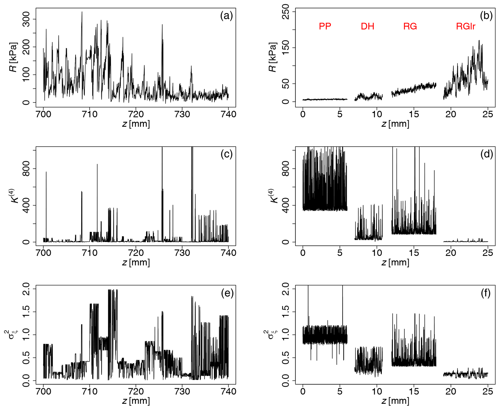
Figure 10The snow hardness profile of a field measurement together with its fourth-order KM coefficients K(4) and the jump amplitude is shown in (a), (c) and (e). These parameters were determined using non-overlapping moving window with 500 data points (2 mm) by means of the Nadaraya–Watson estimator. Snow hardness profiles of the laboratory-prepared snow types and their local parameters are also plotted to enable better comparison (b, d, f); they are shifted horizontally for better visualization. The results of field measurements are shown at the depth of . With reference to the local characteristic snow types from laboratory measurements, we can see in the dynamics that mixtures of different snow types are present in this section of measurement. For , the high K(4) and indicate the presence of small and less dense structures of snow which resemble the RG-like snow types.
Our work is based on the proposed analogy of Brownian motion and the SMP penetration process, as illustrated in Fig. 1. The events of bond breaking or of collision with molecules are summed up in a mean force and noise. For continuous Brownian noise, we need an integration over sufficient micro-scale events, as discussed by Einstein (1905) in his original paper. In our interpretation, it is found that sufficiently large particles lead to this integration; see Fig. 1b. To our interpretation, this integration over discrete single events of bond breaking in the immediate surroundings of the SMP, in addition to the pushing aside of loose snow grains during the penetration process, forms continuous Brownian noise. The jump noise may represent the bond-breaking events occurring directly at the tip of the SMP, and the amplitude of the jump noise should depend on the strength of the ice bonds and void sizes. From this interpretation, it is clear that snow type morphology, shown in Fig. 4, is essential for effective stochastic analysis as outlined herein.
We start the discussion with the mean values of R and the standard deviation σR (see Fig. 6 and Table 1). The less dense PP and the dense RGlr snow can be well separated, whereas the differences are less clear for DH and RG. In the following, we discuss the measured SMP penetration profiles based on our stochastic results. Since we now focus on a stochastic investigation of the fluctuations in the penetration profiles, the detrended and normalized data are R′ used. Furthermore, we can note that the normalization of the snow profiles affects neither the correlation length scales from the drift coefficients nor the jump characteristic length scales . Because this analysis depends on the number of available data, our discussion of the estimated KM coefficients is limited to the range .
The drift terms D(1), Fig. 8, are all monotonously decaying with increasing R′ and can be approximated by a linear decay, . The slope indicates how fast the signals relax to a fixed point located at . The magnitudes of the slopes are PP > RG > DH > RGlr; thus the PP snow has the fastest relaxation or shortest correlation length scale LC. We find that the larger the ice structures, the slower (or longer) the relaxation. If we compare this result with the snow structures shown in Fig. 4, we conclude that LC or γ is clearly related to the size of the snow structures.
The results for D(2) show that about the same diffusive noise amplitude is found for all snow types. In contrast, we see clear differences for the fourth-order KM coefficients K(4). Although K(4)≠0 is always the case, clear differences in the magnitude of this KM coefficient are found. K(4) is the largest in PP, followed by RG, DH and RGlr.
The amplitudes of jump noise, , are the highest for PP, followed by RG, DH and RGlr. For the jump probabilities λ Δz, we distinguish a group composed of PP and RG, with higher values, and one composed of DH and RGlr, with lower values. One can interpret this finding such that for the precipitation particles (PP, recent snow) with very small ice structures and high porosity, the breaking occurs easily and frequently, which explains that the jump probability has the largest contribution here. Similarly, RG is also less dense with smaller ice structures than DH and RGlr. Thus, we can also interpret this finding such that the smaller the ice structures and the less densely the snow is packed, the stronger the jump noise. For the densely packed snow with larger ice structures, the breaking of the ice structures is less frequent, which explains a lower jump probability. The mean of the jump rate in the range of can be used to define the second characteristic length scale . Similarly to the correlation length scale , PP has the smallest length, followed by RG, DH and RGlr.
Besides the features of the different terms in the stochastic processes, the contributions of the diffusive and the jump noise can be compared by the dimensionless quotient of , i.e., the relation between the two noise contributions. Consistent with our earlier discussion, the smallest values for are obtained for PP; i.e., the jump noise dominates due to the frequent fracture of small (soft) ice structures. For the other snow types, we see that within the range of , the values of increase with larger ice structures, in accordance with Fig. 4. The quotient is smaller for PP and RG and larger for DH and RGlr. For RGlr, the diffusive noise dominates in a broad range of R′ values. For the densely packed snow with larger grain sizes, it also takes much force to push the ice grains on the side but not necessarily to break the cohesive bonds close to the tip. Therefore the penetration signal is dominated by Brownian noise. This result is also consistent with the value of K(4), which is relatively small for RGlr. It is interesting to see that and K(4) enable differentiation between RG and DH. In contrast, according to the classical statistical features of the snow signals shown in Table 1, the differences for DH and RG are less clear.
In Sect. 3.2, we analyze field measurement data which are highly inhomogeneous. With reference to the laboratory measurements, we see dynamics that suggest mixtures of different snow types within this depth segment. For , the high K(4) and indicate the presence of small and less dense structures of snow which resemble the RG-like snow types. Based on these preliminary results of real field data, the developed methodology appears promising for interpreting cone penetration tests in the field, but further quantitative evaluation is required.
In conclusion, we observe that the advanced stochastic analysis of SMP measurements of snow layers allows differentiation of snow types. The diffusive and jump-noise contribution can be quantified and gives new insights into the stochastic behaviors of the cone penetration test in snow. For different snow types, we find an interesting mixture of diffusive- and jump-like noise. We propose the interpretation that the dominant diffusive process is due to the pushing aside of many snow grains, whereas the breaking of ice structures leads to dominant jump noise. Our results show that the denser structures typical of DH and RGlr lead to a more collective diffusive behavior, whereas for the highly porous snow structures of PP and RG, the single breaking events lead to a relatively strong jump noise. For this interpretation, all R values were detrended and normalized; thus the absolute values of the snow hardness R are not essential but more the resulting collective behavior of the snow types.
Finally, we would like to point out that our characterization of a complex material, snow, by a penetration process should have the potential to be generalized to, for example, biological tissue or ground layers. Last but not least, we would like to point out that our work provides additional insight into analyzing and modeling the complex nature of snow types, complementing existing methods.
All the data and codes can be found under https://doi.org/10.5281/zenodo.7358919 (pplin13, 2022).
PPL did the preliminary analysis of the data and simulations and wrote the main part of the manuscript. PH and IP performed the experiments. JP had the initial idea, and JP, MW and MRRT supervised the work. All the authors interpreted the results and helped in preparing and editing the manuscript.
The contact author has declared that none of the authors has any competing interests.
Publisher’s note: Copernicus Publications remains neutral with regard to jurisdictional claims in published maps and institutional affiliations.
The authors would like to thank Christian Behnken and Hauke Hähne for helpful discussions.
This research has been supported by the European Space Agency (grant no. 4000112698/14/NL/LvH) and the Agence Nationale de la Recherche (grant no. ANR10 LABX56).
This paper was edited by Melody Sandells and reviewed by Henning Löwe and Adrian McCallum.
Anvari, M., Rahimi Tabar, M., Peinke, J., and Lehnertz, K.: Disentangling the stochastic behaviour of complex time series, Nature Scientific Reports, 6, 35435, https://doi.org/10.1038/srep35435, 2016. a, b, c, d
Bader, H. and Niggli, P.: Der Schnee und seine Metamorphose: Erste Ergebnisse und Anwendungen einer systematischen Untersuchung der alpinen Winterschneedecke. Durchgeführt von der Station Weissfluhjoch-Davos der Schweiz. Schnee- und Lawinenforschungskommission 1934–1938, Kümmerly and Frey, https://books.google.de/books?id=-2V8RQAACAAJ (last access: 25 November 2022), 1939. a
Bandi, F. M. and Nguyen, T. H.: On the functional estimation of jump-diffusion models, J. Econometrics, 116, https://doi.org/10.1016/S0304-4076(03)00110-6, 293–328, 2003. a
Calonne, N., Richter, B., Löwe, H., Cetti, C., ter Schure, J., Van Herwijnen, A., Fierz, C., Jaggi, M., and Schneebeli, M.: The RHOSSA campaign: multi-resolution monitoring of the seasonal evolution of the structure and mechanical stability of an alpine snowpack, The Cryosphere, 14, 1829–1848, https://doi.org/10.5194/tc-14-1829-2020, 2020. a
Colbeck, S., Akitaya, E., Armstrong, R., Gubler, H., Lafeuille, J., Lied, K., Mcclung, D., and Morris, E.: The International Classification for Seasonal Snow on the Ground, The International Commission on Snow and Ice of the International Association of Scientific Hydrology, https://books.google.de/books?id=uwImvwEACAAJ (last access: 25 November 2022), 1990. a
Einstein, A.: Über die von der molekularkinetischen Theorie der Wärme geforderte Bewegung von in ruhenden Flüssigkeiten suspendierten Teilchen, Ann. Phys., 17, 549, DOI https://doi.org/10.1002/andp.2005517S112, 1905. a, b
Fierz, C., Armstrong, R. L., Durand, Y., Etchevers, P., Greene, E., McClung, D. M., Nishimura, K., Satyawali, P. K., and Sokratov, S. A.: The International Classification for Seasonal Snow on the Ground, IHP-VII Technical Documents in Hydrology No. 83, IACS Contribution No. 1, UNESCO-IHP, Paris, https://unesdoc.unesco.org/ark:/48223/pf0000186462 (last access: 25 November 2022), 2009. a, b
Friedrich, R., Peinke, J., Sahimi, M., and Reza Rahimi Tabar, M.: Approaching complexity by stochastic methods: From biological systems to turbulence, Phys. Rep., 506, 87–162, https://doi.org/10.1016/j.physrep.2011.05.003, 2011. a, b, c, d
Gardiner, C.: Handbook of Stochastic Methods for Physics, Chemistry, and the Natural Sciences, Proceedings in Life Sciences, Springer-Verlag, https://books.google.de/books?id=cRfvAAAAMAAJ (last access: 25 November 2022), 1985. a
Hagenmuller, P. and Pilloix, T.: A New Method for Comparing and Matching Snow Profiles, Application for Profiles Measured by Penetrometers, Front. Earth Sci., 4, 52, https://doi.org/10.3389/feart.2016.00052, 2016. a
Hanson, F.: Applied Stochastic Processes and Control for Jump Diffusions: Modeling, Analysis, and Computation, Advances in Design and Control, Society for Industrial and Applied Mathematics, https://doi.org/10.1137/1.9780898718638, 2007. a
Isserlis, L.: On certain probable errors and correlation coefficients of multiple frequency distributions with skew regression, Biometrika, 11, 185–190, https://doi.org/10.1093/biomet/11.3.185, 1916. a
Johannes, M.: The Statistical and Economic Role of Jumps in Continuous-Time Interest Rate Models, J. Financ., 59, https://doi.org/10.1111/j.1540-6321.2004.00632.x, 227–260, 2004. a
Johnson, J. B. and Schneebeli, M.: Characterizing the microstructural and micromechanical properties of snow, Cold Reg. Sci. Technol., 30, 91–100, https://doi.org/10.1016/S0165-232X(99)00013-0, 1999. a, b, c, d, e
Lamouroux, D. and Lehnertz, K.: Kernel-based regression of drift and diffusion coefficients of stochastic processes, Phys. Lett. A, 373, 3507–3512, https://doi.org/10.1016/j.physleta.2009.07.073, 2009. a
Löwe, H. and van Herwijnen, A.: A Poisson shot noise model for micro-penetration of snow, Cold Reg. Sci. Technol., 70, 62–70, https://doi.org/10.1016/j.coldregions.2011.09.001, 2012. a, b, c, d, e, f
Marshall, H. and Johnson, J.: Accurate Inversion of High-Resolution Snow Penetrometer Signals for Microstructural and Micromechanical Properties, J. Geophys. Res., 114, F04016, https://doi.org/10.1029/2009JF001269, 2009. a
McCallum, A.: Cone Penetration Testing (CPT): a valuable tool for investigating polar snow, J. Hydrol., 52, 97–113, https://www.jstor.org/stable/43945048 (last access: 29 November 2022), 2013. a
Nadaraya, E. A.: On Estimating Regression, Theor. Probab. Appl., 9, 141–142, https://doi.org/10.1137/1109020, 1964. a
Pawula, R. F.: Approximation of the Linear Boltzmann Equation by the Fokker-Planck Equation, Phys. Rev., 162, 186–188, https://doi.org/10.1103/PhysRev.162.186, 1967. a
Peinke, I., Hagenmuller, P., Chambon, G., and Roulle, J.: Investigation of snow sintering at microstructural scale from micro-penetration tests, Cold Reg. Sci. Technol., 162, 43–55, https://doi.org/10.1016/j.coldregions.2019.03.018, 2019. a, b, c, d, e
Peinke, I., Hagenmuller, P., Andò, E., Chambon, G., Flin, F., and Roulle, J.: Experimental Study of Cone Penetration in Snow Using X-Ray Tomography, Front. Earth Sci., 8, 63, https://doi.org/10.3389/feart.2020.00063, 2020. a, b, c, d
pplin13: pplin13/Snow_RCodes: Stochastic analysis of micro-cone penetration tests in snow (v0.1.0), Zenodo [code], https://doi.org/10.5281/zenodo.7358919, 2022. a
Proksch, M., Löwe, H., and Schneebeli, M.: Density, specific surface area, and correlation length of snow measured by high-resolution penetrometry, J. Geophys. Res.-Earth, 120, 346–362, https://doi.org/10.1002/2014JF003266, 2015. a
Reuter, B., Schweizer, J., and van Herwijnen, A.: A process-based approach to estimate point snow instability, The Cryosphere, 9, 837–847, https://doi.org/10.5194/tc-9-837-2015, 2015. a
Reuter, B., Proksch, M., Löwe, H., van Herwijnen, A., and Schweizer, J.: Comparing measurements of snow mechanical properties relevant for slab avalanche release, J. Glaciol., 65, 55–67, https://doi.org/10.1017/jog.2018.93, 2019. a
Rinn, P., Lind, P. G., Wächter, M., and Peinke, J.: The Langevin Approach: An R Package for Modeling Markov Processes, Journal of Open Research Software, 4, e34, https://doi.org/10.5334/jors.123, 2016. a, b
Risken, H.: Fokker-Planck Equation, Springer Berlin Heidelberg, Berlin, Heidelberg, 63–95, https://doi.org/10.1007/978-3-642-96807-5_4, 1984. a, b
Schneebeli, M., Pielmeier, C., and Johnson, J. B.: Measuring snow microstructure and hardness using a high resolution penetrometer, Cold Reg. Sci. Technol., 30, 101–114, https://doi.org/10.1016/S0165-232X(99)00030-0, 1999. a, b
Schweizer, J., Jamieson, B., and Schneebeli, M.: Snow avalanche formation, Rev. Geophys., 41, 1016, https://doi.org/10.1029/2002RG000123, 2003. a
Stanton, R.: A Nonparametric Model of Term Structure Dynamics and the Market Price of Interest Rate Risk, J. Financ., 52, 1973–2002, https://econpapers.repec.org/RePEc:bla:jfinan:v:52:y:1997:i:5:p:1973-2002 (last access: 29 November 2022), 1997. a
Tabar, M. R. R.: Analysis and Data-Based Reconstruction of Complex Nonlinear Dynamical Systems: Using the Methods of Stochastic Processes, Springer, Cham-Switzerland, https://doi.org/10.1007/978-3-030-18472-8, 2019. a, b, c, d, e, f
Tankov, P.: Financial Modelling with Jump Processes, Chapman and Hall/CRC Financial Mathematics Series, CRC Press, https://doi.org/10.1201/9780203485217, 2003. a
Watson, G. S.: Smooth Regression Analysis, Sankhyā Ser. A, 26, 359–372, https://www.jstor.org/stable/25049340 (last access: 29 November 2022), 1964. a
Wick, G. C.: The Evaluation of the Collision Matrix, Phys. Rev., 80, 268–272, https://doi.org/10.1103/PhysRev.80.268, 1950. a
A direct comparison of our stochastic approach with the works based on shot noise is out of the scope of this paper.
KM coefficients for the Langevin equation are defined as in Friedrich et al. (2011) and Rinn et al. (2016). In order to make it consistent with the jump-diffusion process, our definition differs by a factor of , in which where 〈Γ(t)〉=0 and . The corresponding Fokker–Planck equation will be .
The results do not change significantly if the kernel widths are changed between 0.14 and 0.66 mm, where this range corresponds to the range of average grain sizes of the snow types.