A random forest model to assess snow instability from simulated snow stratigraphy

Modeled snow stratigraphy and instability data are a promising source of information for avalanche forecasting. While instability indices describing the mechanical processes of dry-snow avalanche release have been implemented into snow cover models, there exists no readily applicable method that combines these metrics to predict snow instability. We therefore trained a random forest (RF) classification model to assess snow instability from snow stratigraphy simulated with SNOWPACK. To do so, we manually compared 742 snow profiles observed in the Swiss Alps with their simulated counterparts and selected the simulated weak layer corresponding to the observed rutschblock failure layer. We then used the observed stability test result and an estimate of the local avalanche danger to construct a binary target variable (stable vs. unstable) and considered 34 features describing the simulated weak layer and the overlying slab as potential explanatory variables. The final RF classifier aggregates six of these features into the output probability P_unstable, corresponding to the mean vote of an ensemble of 400 classification trees. Although the subset of training data only consisted of 146 profiles labeled as either unstable or stable, the model classified profiles from an independent validation data set (N=121) with high reliability (accuracy 88 %, precision 96 %, recall 85 %) using manually predefined weak layers. Model performance was even higher (accuracy 93 %, precision 96 %, recall 92 %), when the weakest layers of the profiles were identified with the maximum of P_unstable. Finally, we compared model predictions to observed avalanche activity in the region of Davos for five winter seasons. Of the 252 avalanche days (345 non-avalanche days), 69 % (75 %) were classified correctly. Overall, the results of our RF classification are very encouraging, suggesting it could be of great value for operational avalanche forecasting.

1 Introduction

Forecasting snow avalanches in mountainous terrain has long proved to be a challenge for researchers and operational forecasters. The probability of avalanche release depends on snow instability, the sensitivity of the local snowpack to artificial or natural triggers (Statham et al., 2018). Snow instability results from a complex interplay between snowpack, terrain and various meteorological drivers over time (e.g., Schweizer et al., 2003a; Reuter et al., 2015b). To estimate snow instability at a specific location, stability tests, such as the rutschblock (RB) test or the extended column test (ECT), can be performed (e.g., Schweizer and Jamieson, 2010; Techel et al., 2020b). These tests consist of incrementally loading an isolated block of snow to assess the load required to fracture weak layers in the snowpack. Such tests provide essential information for the preparation of avalanche forecasts intended to warn the public about the avalanche danger. However, stability tests are very time-consuming, sometimes dangerous to perform and only provide local information for one point in time. Although the potential of numerical snow cover models to increase the spatial and temporal resolution of snow instability data has been recognized, operational avalanche forecasting rarely incorporates modeled snow instability data (Morin et al., 2020).

A major reason for the limited use of modeled snow instability data in avalanche forecasting is the complexity of the processes involved in avalanche formation. The release of a dry-snow slab avalanche is a fracture mechanical process starting with failure initiation in a weak layer below a cohesive slab and followed by rapid crack propagation across the slope (e.g., Schweizer et al., 2003a; van Herwijnen and Jamieson, 2007; Gaume et al., 2017). Modeling snow instability thus requires (i) modeling snow stratigraphy including relevant weak layers, (ii) suitable parameters describing the mechanical processes and (iii) a meaningful interpretation of these parameters. Modeling the one-dimensional snow stratigraphy (step i) is feasible with the two most advanced numerical snow cover models CROCUS (Brun et al., 1989, 1992; Vionnet et al., 2012) and SNOWPACK (Lehning et al., 1999; Bartelt and Lehning, 2002; Lehning et al., 2002a, b). Both physically based models are driven with meteorological data from either automatic weather stations or numerical weather prediction models (e.g., Bellaire and Jamieson, 2013; Quéno et al., 2016) and provide microstructural (e.g., grain size) and macroscopic (e.g., density) properties for each snow layer. Validation campaigns have demonstrated a reasonably good agreement between modeled and observed snow stratigraphy (e.g., Durand et al., 1999; Lehning et al., 2001; Monti et al., 2009; Calonne et al., 2020) and, in particular, have confirmed the models' capability to reproduce critical snow layers such as surface hoar (Bellaire and Jamieson, 2013; Horton et al., 2014; Viallon-Galinier et al., 2020). From the basic model output, different mechanical properties can be calculated. The model MEPRA combines mechanical variables obtained from CROCUS snow cover simulations with empirical rules into an index describing avalanche danger (Giraud, 1993). SNOWPACK contains a module for mechanical stability diagnostics which includes various parameters describing the processes of avalanche formation. To assess dry-snow instability, a potential weak layer is determined with the structural stability index (SSI; Schweizer et al., 2006) or the threshold sum approach (Monti et al., 2014), and stability indices are then calculated for this layer. These include the skier stability index (SK₃₈) describing failure initiation (Föhn, 1987b; Jamieson and Johnston, 1998; Monti et al., 2016) and the recently implemented critical cut length (r_c) relating to crack propagation (Gaume et al., 2017; Richter et al., 2019). While SK₃₈ and r_c should capture the most important processes involved in the formation of human-triggered avalanches (step ii), the interpretation of these stability indices (step iii) remains challenging. Although both indices were related to avalanche observations or signs of instability in several field studies using observed snow properties (e.g., Jamieson and Johnston, 1998; Gauthier and Jamieson, 2008; Reuter and Schweizer, 2018), there are only a few validation studies based on simulated snow stratigraphy (e.g., Schweizer et al., 2006; Richter et al., 2019). In particular, there are no validated threshold values for a combination of both indices in the case of simulated snow profiles. Moreover, SK₃₈ provides meaningful results only for weak layers that are not deeply buried (< 80 cm) (Schweizer et al., 2016; Richter et al., 2021).

Given the limitations of the process-based snow instability indices, we aim at assessing dry-snow instability from simulated snow stratigraphy employing a machine learning approach. Our goal is to develop a model which aggregates information on snow stratigraphy into a probability of instability provided for each layer of the simulated snow profile. This model should offer the possibility of detecting the weakest layer of a snow profile and assessing its degree of instability with one single index. To this end, we incorporate existing stability indices as well as microstructural and macroscopic snow layer properties as input variables into a random forest (RF) classification model. We construct this RF model using a one-to-one comparison of SNOWPACK simulations with observed snow profiles including stability test results. To discriminate rather unstable from rather stable snow conditions, we derive threshold values for the predicted probability of instability. A comparison of modeled snow instability with observed avalanche activity highlights the potential of our model to assess snow instability.

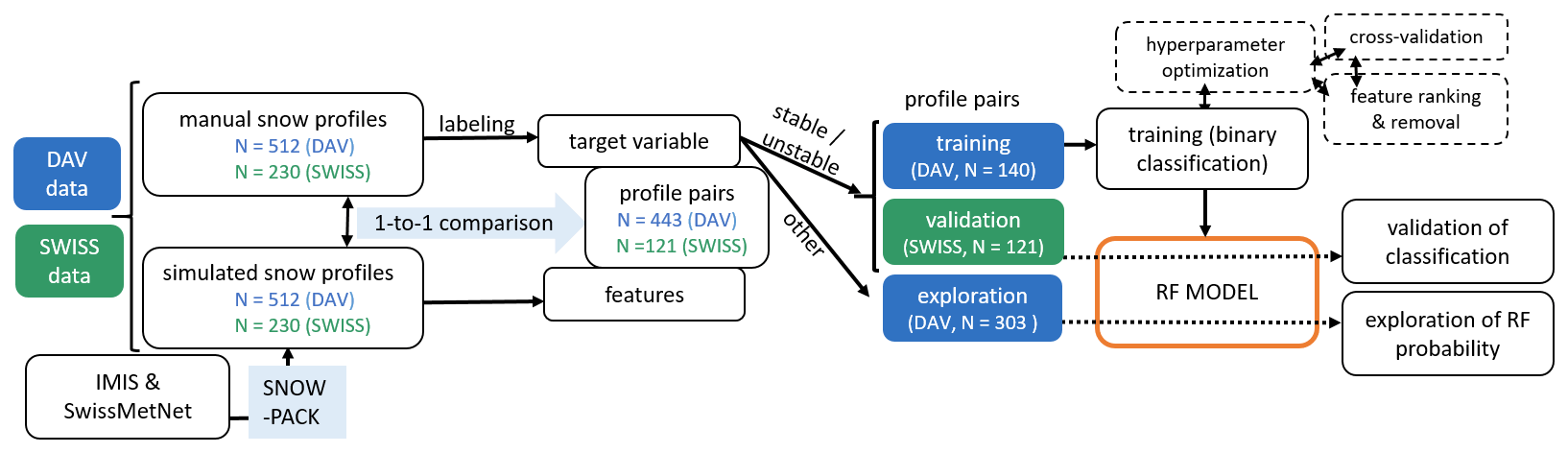
Figure 1 Overview of data sets and steps used for data pre-processing (left side) and model training and evaluation (right side).

2 Data and data preparation

Our approach to classifying snow profiles using simulated snow stratigraphy was divided into several steps (Fig. 1). It involved two data sets (DAV and SWISS), each consisting of pairs of observed snow profiles (Sect. 2.1) and associated simulations at virtual slopes. The simulations were obtained using meteorological forcing data (Sect. 2.2) as input for SNOWPACK (Sect. 2.3). Pre-processing the data included a one-to-one comparison of manual and simulated snow profiles. We manually defined a weak layer in the SNOWPACK simulations corresponding to the rutschblock failure layer observed in the field and discarded all profile pairs that did not meet predefined similarity criteria (Sect. 3.1.2). We then used the DAV data set to train the classification model (Sect. 3.1.3) and the SWISS data set for validation (Sect. 3.2).

2.1 Manual snow profiles and stability observations

2.1.1 DAV data set

To train our classification model, we used snow profiles observed in the region of Davos (Eastern Swiss Alps, Switzerland; Appendix A – Figs. A1 and A2) from 18 winter seasons between 2001/02 and 2018/19 (data set used by Schweizer et al., 2021b, accessible at Schweizer et al., 2021a). This data set (DAV) consisted of 512 profiles with information on the profile site (coordinates, slope angle, slope aspect), snow stratigraphy (grain type and size, snow hardness index) observed according to Fierz et al. (2009), a rutschblock test (RB; Föhn, 1987a; Schweizer and Jamieson, 2010) and an estimate of the local avalanche danger level (local nowcast – LN; Techel and Schweizer, 2017). RB test results included the test score (ranging from 1 to 7; for a detailed description of the test procedure see Schweizer, 2002), depth of the failure interface and release type (whole block, partial release below skis or only an edge). A local nowcast assessment of avalanche danger was also provided using a five-level danger scale (1 – low, 2 – moderate, 3 – considerable, 4 – high, 5 – very high). The assessment refers to the area observed during a day traveling in the backcountry, which is typically on the order of several square kilometers, and does not refer to a single slope (for more details refer to Techel and Schweizer, 2017). The mean snow depth of all profiles in the DAV data set was 111 cm, and 76 % of the recorded failure layers contained persistent grain types.

To evaluate the application of the RF model to complete snow profiles, we also used visual observations of dry-snow avalanches from the region of Davos for the five winter seasons 2014/15 until 2018/19 (data set used by Schweizer et al., 2020a, and accessible at Schweizer et al., 2020b). From this data set, we extracted dry-snow avalanches which released naturally, were human-triggered or had an unknown trigger type. These data were aggregated into the avalanche activity index (AAI), a weighted sum of all observed avalanches on a specific day, with weights assigned according to avalanche size (weights 0.01, 0.1, 1 and 10 for size classes 1 to 4, respectively;  Schweizer et al., 2003b) and type of triggering (weights 1, 0.81 and 0.5 for trigger types “natural”, “unknown” and “human”, respectively;  Schweizer et al., 2020a). We further defined an avalanche day as a day with at least one recorded avalanche of size class 2 or greater.

2.1.2 SWISS data set

For model validation, we compiled an independent data set of 230 snow profiles (SWISS, Fig. A1), again including a RB test and a LN assessment. These profiles were observed at various locations throughout the Swiss Alps, not including the region of Davos, during the winter seasons of 2001/02 to 2018/19. To perform representative SNOWPACK simulations, we only used snow profiles within a horizontal distance of 10 km and a vertical distance of 200 m of an automated weather station (AWS). Moreover, the data recorded by the corresponding AWS could not have gaps of more than 24 h. The mean snow depth of the SWISS profiles was 138 cm, and 49 % of the RB failure interfaces were located adjacent to a layer of persistent grain types.

2.2 Meteorological forcing data

To simulate the snow cover at the locations of the observed snow profiles, we forced SNOWPACK with meteorological data from a network of automated weather stations (AWSs) located between 1500 and 3000 $\mathrm{m}\mathrm{a}.\mathrm{s}.\mathrm{l}.$ across the Swiss Alps (Intercantonal Measurement and Information System – IMIS; Lehning et al., 1999). These IMIS stations are located at mostly flat sites considered representative of the surrounding area. Meteorological variables and snow cover properties were recorded every 30 min and included air temperature (non-ventilated), relative humidity, wind speed and direction, reflected shortwave radiation, snow surface temperature, and snow height. The majority of the AWSs are equipped with an unheated rain gauge and thus do not provide reliable measurements of solid precipitation. For the simulations of the DAV data set, we also used data from two SwissMetNet stations, operated by the Swiss Federal Office of Meteorology and Climatology (MeteoSwiss) and a research station operated by SLF. These stations also measure incoming short- and longwave radiation with ventilated and heated sensors as well as solid and liquid precipitation with heated rain gauges.

2.3 SNOWPACK setup

2.3.1 DAV data set

For the SNOWPACK simulations in the DAV data set, we interpolated measurements from six AWSs from the IMIS network (WFJ2, DAV2, DAV3, KLO2, KLO3, SLF2), two SwissMetNet stations (WFJ, DAV) and the research station STB2 to the locations of the snow profiles. For the locations of snow profiles and AWSs see Appendix A (Figs. A1 and A2). In addition to the precipitation measurements from WFJ and DAV, we also used estimated precipitation values for the five IMIS stations obtained from SNOWPACK runs driven with measured snow depth (Lehning et al., 2002a; Wever et al., 2015), employing an empirical relationship for new-snow density as a function of air temperature, relative humidity and wind speed (Schmucki et al., 2014). To spatially interpolate meteorological parameters to the locations of the manual snow profiles, we used the pre-processing library MeteoIO, which applies a combination of lapse rate and inverse distance weighting (Bavay and Egger, 2014).

Starting on 1 October of the respective winter season, each simulation was run at the location of the manual snow profile up to the exact date and time (± 0.5 h) when the profile was observed, using a time step size of 15 min. To account for slope angle and aspect, the simulations were carried out for so-called virtual slopes; i.e., shortwave radiation and precipitation amounts were projected onto the slope, while other influences of surrounding terrain were neglected. Energy fluxes at the snow–atmosphere interface were calculated using Neumann boundary conditions. For the soil heat flux at the bottom of the snowpack we employed a constant value of 0.06 W m⁻² (Davies and Davies, 2010). The flow of liquid water through the snow cover was modeled applying the Richards equation (Wever et al., 2014). Finally, to obtain a simulated snow depth close to that of the manual snow profile, we scaled interpolated precipitation values as

$$\begin{array}{}\text{(1)}& P_{\text{corr},i}\left(t\right)={\displaystyle \frac{{\text{HS}}_{\text{obs},i}}{{\text{HS}}_{\mathrm{1},i}}}{P}_{\mathrm{1},i}\left(t\right),\end{array}$$

where P_corr,i(t) is the scaled precipitation for profile i at time step t, HS_obs,i is the snow depth observed at the manual profile i, HS_1,i is the simulated snow depth from a first unscaled SNOWPACK run for the same location and time as the observed profile, and P_1,i(t) is the interpolated unscaled precipitation used in the first simulation. Each simulation was then re-run using the corrected precipitation P_corr,i(t) to drive snow accumulation.

2.3.2 SWISS data set

For the SWISS data set, we simulated snow stratigraphy at the location of the nearest IMIS station. In contrast to the DAV data set, we thus did not interpolate meteorological data to the exact profile location. As with the DAV data set, we performed virtual slope simulations with slope angle and aspect corresponding to the manual profile. The measured snow surface temperature was imposed as a Dirichlet-type upper boundary condition for the energy exchange at the snow surface. To ensure that the energy input was not underestimated during ablation periods, the upper boundary condition switched to Neumann-type (i.e., energy fluxes at the snow surface were calculated) whenever the snow surface temperature exceeded −1.0 ^∘C. All further settings, including the scaling of precipitation, were identical to those of the DAV simulations.

3 Methods

An overview of the different steps and data subsets involved in the development (Sect. 3.1) and evaluation (Sect. 3.2) of our classification model is shown on the right-hand side of Fig. 1.

3.1 Model development and optimization

3.1.1 Target variable and features

The construction of the classification model required the definition of a target variable based on the observed stability. To this end, we labeled the manual snow profiles based on the RB test results and the LN assessment. The snow profile and the RB test provide information on weak layers and their stability at the location of the snow pit. The location of these snow pits is often rather specific as observers aim to find locations where snowpack stability is poor (e.g., McClung, 2002). The nowcast assessment (LN), on the other hand, also considers observations at a larger scale, such as recent avalanches, avalanche size and signs of instability (Schweizer et al., 2021b).

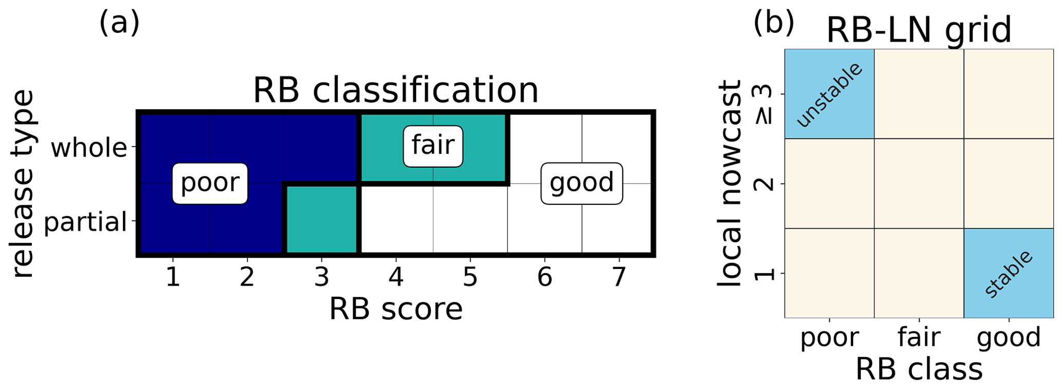
Figure 2 (a) Definition of the RB stability classes poor, fair and good in dependence on RB score and release type. (b) Classification of profiles into nine classes of a rutschblock stability–local nowcast (RB–LN) grid. The classification model was trained on DAV profiles belonging to either the upper-left or the lower-right classes (in blue).

Based on the combination of RB score and release type, we grouped RB test results into three different stability classes: poor, fair and good (Fig. 2a). While our approach is similar to that of Techel et al. (2020b), we only defined three classes by merging the two lowest classes very poor and poor of Techel et al. (2020b) into one class (poor). Besides this RB stability rating, we also considered LN as a second criterion to identify profiles that were presumably most representative of snow stability in the region and hence best suited for building the classification model. The frequency of the different stability classes varies with the danger level (Techel et al., 2020a). If a stability test belongs to a minority class at a given danger level, the simulated snow stratigraphy will likely not be able to reproduce the snowpack at that test location. In general, we cannot expect that the simulated snowpack can fully reproduce the snow depth, stratigraphy and stability as observed at the location of the manual snow profile, since we relied on interpolations of meteorological data to drive the 1D simulations (see Sect. 2.3), which, for instance, do not consider snow redistribution by wind in complex terrain. Therefore, we combined the RB stability classification and the LN assessment and assigned all snow profiles to nine different subgroups (Fig. 2b), of which only two were used to train the classification model. In the following, we denote the upper left and lower right of this 3 × 3 RB–LN grid as stable and unstable classes, respectively; i.e.,

$$\begin{array}{}\text{(2)}& {\displaystyle }\text{stable class}& {\displaystyle }=\left[\right(\text{RB result}=\text{good}\left)\text{ and }\right(\text{LN}=\mathrm{1}\left)\right],\text{(3)}& {\displaystyle }\text{unstable class}& {\displaystyle }=\left[\right(\text{RB result}=\text{poor}\left)\text{ and }\right(\text{LN}\ge \mathrm{3}\left)\right].\end{array}$$

For these two “extreme” classes, we hypothesize that it is more likely that the simulated snow stratigraphy and the manual snow profile are similar compared to all other classes. The two classes stable and unstable thus constituted the binary target variable of our classification model. To train the classification model, we only used the subset of profiles from the DAV data set that belonged to these two classes. The remaining classes were used for model evaluation beyond binary classification. The SWISS data set, on the other hand, only contained profiles labeled as either stable or unstable.

A careful selection and creation of discriminant features are crucial to the predictive performance of any classification task (Duboue, 2020). For our classification model, we extracted features from the simulated snow stratigraphy describing the weak layer and the overlying slab. Overall, we used 34 features (see Appendix B, Table B1), either direct SNOWPACK output, such as macroscopic (e.g., density) or microscopic (e.g., grain size) layer properties, mechanical properties (e.g., shear strength), and stability indices (e.g., SK₃₈), or derived properties (e.g., skier penetration depth) and variables constructed on the basis of expert knowledge (e.g., the mean of the ratio of density and grain size of all slab layers).

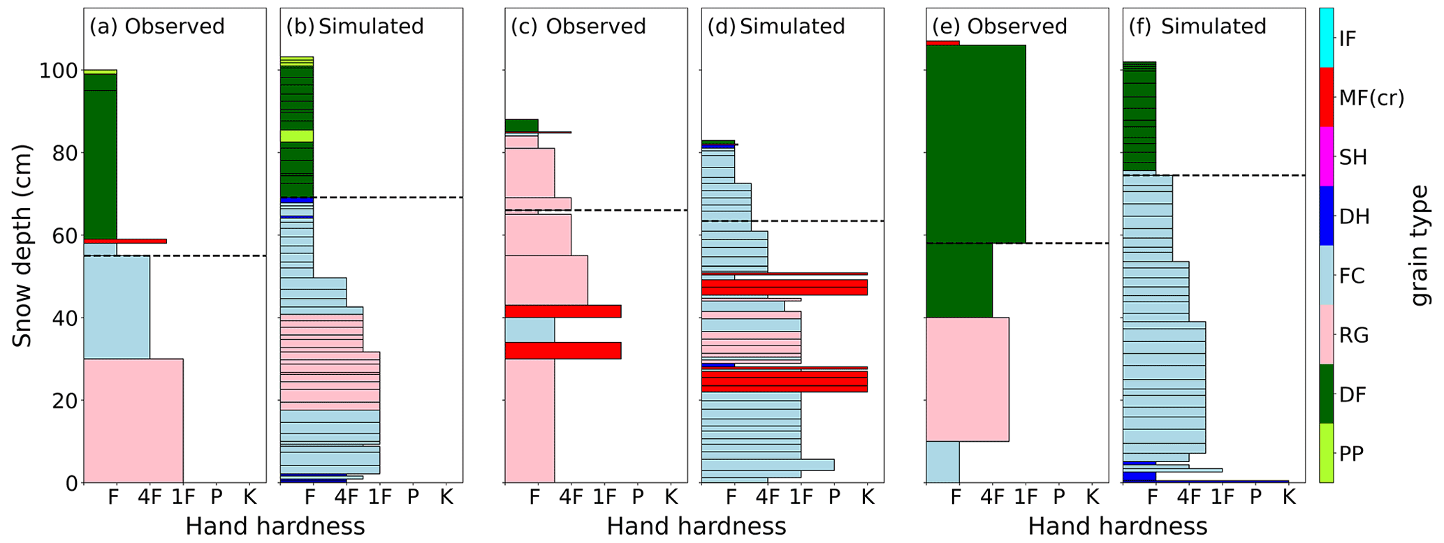
Figure 3 Exemplary profile pairs from the DAV data set with (a, c, e) manually observed snow profiles and (b, d, f) corresponding simulated snow stratigraphy from SNOWPACK. Hand hardness and grain type (colors) were coded after Fierz et al. (2009), where F corresponds to fist, 4F to four fingers, 1F to one finger, P to pencil and K to knife. Grain types are precipitation particles (PP), decomposing and fragmented precipitation particles (DF), rounded grains (RG), faceted crystals (FC), depth hoar (DH), surface hoar (SH), melt forms (MF), melt–freeze crusts (MFcr), and ice formations (IF). The dashed horizontal line in the manual profile displays the observed height of the RB failure layer, and the corresponding manually determined layer is indicated by a dashed line in the respective simulated profile. Profile pairs (a, b) and (c, d) passed the similarity check, while profile pair (e, f) was sorted out. Observed rutschblock results were (a) RB score 1, whole block; (b) RB score 5, edge; and (c) RB score 4, whole block. The local nowcasts were given by (a) LN=3, (b) LN=1 and (c) LN=2.

3.1.2 Profile comparison

For each simulated profile (DAV and SWISS), we manually selected the layer corresponding to the RB failure layer in the manual snow profile. This was done by visually identifying a simulated weak layer with similar grain type and hardness to the RB failure layer, taking into account the overall sequence of layers. Prominent hardness differences and layers consisting of depth hoar, surface hoar or crusts generally facilitated the subjective profile alignment (some examples in Fig. 3). For an unstable profile pair, we always searched for a layer with properties characteristic of a typical failure layer (large grain size, low density, persistent grain type, etc.; see Schweizer and Jamieson, 2003). As simulated snow profiles generally consist of more layers than manual profiles, we chose the layer with the lowest density and largest grain size within the potential layers to define the weak layer. If the weak layer of the manual profile was not present in the simulation, we picked an alternative weak layer within the modeled profile that corresponded best. For instance, in the profile pair in Fig. 3a, we selected the depth hoar layer just below the slab in the simulated profile since the simulation did not contain a faceted layer below a crust as in the observed profile. For stable profile pairs, it was often not possible to find a layer with the same grain type and hardness as the RB failure layer. In that case, we chose a layer with similar properties to the observed layer (e.g., Fig. 3b), rather than selecting a layer with typical weak layer properties. Clearly, the described matching approach is rather subjective and does not lead to an unambiguous choice of the weak layer in the simulated profile. To reduce subjectivity in the comparison of profiles, we adhered to the following criteria:

1. Difference in observed and simulated snow depth must not exceed 20 cm.

2. Simulated slab thickness must not deviate more than 20 cm from the observed slab thickness.

3. The difference in the hand hardness index between the observed and simulated weak layer must not exceed one step.

4. Differences in observed and simulated mean slab hardness must not exceed one step.

5. The grain type in the observed and simulated weak layer must be either both persistent (i.e., facets, surface hoar or depth hoar) or both non-persistent.

A pair of profiles was included if both criterion 1 and criterion 2 and at least two out of the three criteria 3 to 5 were fulfilled. For the profiles where the RB test did not fail at all (i.e., RB score 7) and there was no estimate for the weakest layer, we judged the similarity of the profile pair comparing snow stratigraphy and selected a weakest layer in the simulation based on expert knowledge.

By applying the similarity criteria 1–5 to the 512 DAV profile pairs, we excluded 69 profile pairs (13 %). The number of profiles in the unstable and stable classes of the DAV data set was reduced to N=73 and N=67, respectively (Fig. 4a). To obtain a balanced training data set, we included three additional layers for each of the two stable profiles with no RB failure (i.e., RB score 7). Of the 230 SWISS profiles, 121 profiles fulfilled the similarity criteria (53 %); 75 were labeled as unstable and 46 as stable (Fig. 4b).

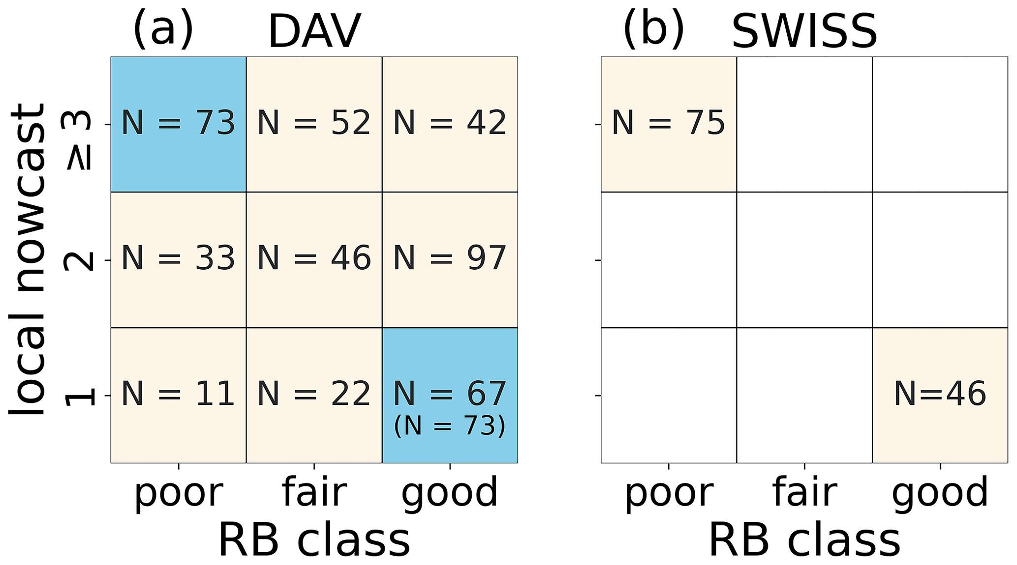
Figure 4 Classification of profiles for (a) the DAV data set and (b) the SWISS data set into RB stability – local nowcast classes. The numbers in the boxes denote the number of profile pairs per class which fulfilled the similarity criteria. The profiles in the blue boxes were used for the training of the classification model, while the beige boxes were used for model evaluation. The second number in the lower-right class, N=73, indicates that we included six additional layers of the stable profiles with RB score 7 to obtain a balanced training data set.

3.1.3 Training the classification model

We trained a RF model to distinguish between stable and unstable profile classes in the DAV data set (N=73 each), using the Python library scikit-learn (Pedregosa et al., 2011). We chose a RF model for this classification task as, in contrast to parametric approaches and threshold-based methods, this model can account for complex mutual dependencies between features without any pre-assumptions about the multi-variable relationship between observed stability and simulated stratigraphy (Breiman, 2001). The RF model is a supervised machine learning algorithm which constructs an ensemble of decision trees for data classification. The average of the predictions from the individual decision trees yields the final prediction of the RF, where the probability for a given class is determined by the proportion of trees that voted for that class. Compared to a single decision tree, a RF estimator is less prone to overfitting as its construction contains several sources of randomness (e.g., bootstrap sampling).

As the variety of split rules used within the ensemble of trees cannot be grasped by the human brain, RF can be considered a black-box-type classifier. Nevertheless, the RF algorithm includes a built-in feature importance estimation, based on evaluating the Gini impurity decrease at each split for every tree in the forest. The importance of a feature is computed as the normalized total decrease in Gini impurity brought by that feature within the ensemble of trees. The more a feature reduces the impurity, the more important the feature is.

The RF model includes several hyperparameters that can be optimized in order to customize the model to the training data, in particular to prevent overfitting. The main hyperparameters include

• the number of trees in the forest

• the maximal depth of a tree, i.e., the longest path between the root node and the leaf node

• the maximal number of features to consider for the best split

• the minimum number of samples required to split a node

• the function to measure the quality of a split.

We optimized the hyperparameters before training the final RF model by systematically considering different hyperparameter combinations in a cross-validated grid search. For every combination of hyperparameter settings, we trained a random forest model on five different subgroups of the training data set and evaluated model accuracy on the left-out data. To prevent similar profiles being used for training and evaluation, we sorted the profiles by date before splitting the data set. We repeated the hyperparameter optimization process with different subsets of the complete set of features, avoiding highly correlated (Pearson's r>0.8) pairs of features. Finally, we selected the combination of hyperparameters and feature subset which yielded the highest mean accuracy score (i.e., the ratio of correct predictions among all predictions) in the 5-fold cross-validation.

Based on the feature importance ranking of the RF model with the optimized hyperparameters, we selected a subset of features with the highest ranking (feature importance > 0.05). We then conducted another round of hyperparameter optimization with the new choice of features (N=6) and trained the final RF model with the optimized hyperparameters on the complete set of training data.

3.2 Model evaluation

3.2.1 Classifier performance on the SWISS data set

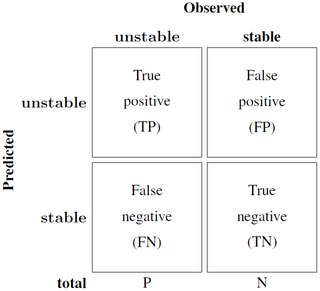
To evaluate the performance of the final RF model, we compared predicted and observed stability classes using the SWISS data set and standard performance measures based on a 2 × 2 contingency table (Fig. 5) (Wilks, 2011). With the definitions shown in the contingency table, the accuracy, precision (positive predictive value), recall (true positive rate or sensitivity) and specificity (true negative rate) are defined as

$$\begin{array}{}\text{(4)}& {\displaystyle }\text{accuracy}& {\displaystyle }={\displaystyle \frac{\text{TP}+\text{TN}}{\mathrm{P}+\mathrm{N}}},\text{(5)}& {\displaystyle }\text{precision}& {\displaystyle }={\displaystyle \frac{\text{TP}}{\text{TP}+\text{FP}}},\text{(6)}& {\displaystyle }\text{recall}& {\displaystyle }={\displaystyle \frac{\text{TP}}{\text{P}}},\text{(7)}& {\displaystyle }\text{specificity}& {\displaystyle }={\displaystyle \frac{\text{TN}}{\text{N}}}.\end{array}$$

Figure 5 Contingency table.

To optimize the classification performance, we analyzed the receiver operating characteristic (ROC) curve (Fawcett, 2006). The ROC curve is a diagnostic plot and shows the recall against the false positive rate ($\text{false positive rate}=\frac{\mathrm{FP}}{N}=\mathrm{1}-\text{specificity}$) for different classification thresholds. A random classifier would yield a diagonal line from [0,0] to [1,1], and a perfect model would be indicated by a ROC curve rising vertically from [0,0] to [0,1] and then horizontally to [1,1]. The area under the ROC curve (AUC) summarizes the overall performance of a model with a value between 0.5 (no skill) and 1.0 (perfect skill). When equal weight is given to recall and specificity, the optimal threshold is the threshold value that maximizes Youden's $J=\text{recall}+\text{specificity}-\mathrm{1}$ statistic, which describes the vertical distance between the [0,0]–[1,1] diagonal and the associated point on the ROC curve (Youden, 1950).

3.2.2 Application to all profile layers

The RF classifier was trained to predict two classes (stable and unstable) for manually identified weak layers. To investigate if the RF model can be used to identify the weakest layer in a simulated snow profile, we analyzed the probability of instability P_unstable given by the mean vote of the RF; i.e.,

$$\begin{array}{}\text{(8)}& P_{\text{unstable}}={\displaystyle \frac{\mathrm{1}}{n_{\text{tree}}}}\sum _{i=\mathrm{1}}^{n_{\text{tree}}}\text{vote}\left({\text{tree}}_i\right),\end{array}$$

where n_tree is the total number of trees in the forest and $\text{vote}\left({\text{tree}}_i\right)\in \mathit{\{}\mathrm{0},\mathrm{1}\mathit{\}}$ is the vote of the ith tree, which is either 0 (stable) or 1 (unstable). Using P_unstable and its overall maximum value P_max=max(P_unstable), we explored the applicability of our RF model to complete snow profiles in four steps:

1. We applied the RF model to all profiles from the DAV data set which passed the similarity check (N=443), including the profiles not used for training, and calculated the mean of P_unstable for the manually identified failure layers of each RB–LN class.

2. To explore if the maximum value of P_unstable can be used to describe the stability if the weak layer is not a priori known, we again classified the SWISS data set profiles using the P_max values instead of the P_unstable values of the manually determined weak layers.

3. We applied the RF model to each layer of all simulated profiles in the DAV and SWISS data sets and evaluated the probability of detecting the manually picked weak layers with the local maxima of P_unstable. A local maximum was defined as a layer whose value of P_unstable is greater than or equal to the P_unstable values of the two layers above and the two layers below the layer. The probability of detection (POD) was then defined as the proportion of weak layers coinciding with one of the three largest local maxima of P_unstable or one of the adjacent layers within 3 cm of these local maxima.

4. We investigated if the daily maximum of P_unstable for five winter seasons (2014/15 and 2018/19) at the AWS Weissfluhjoch (2536 $\mathrm{m}\mathrm{a}.\mathrm{s}.\mathrm{l}.$) was related to avalanche observations from the region of Davos. To this end, we compared the distributions of the values of P_max on avalanche days and non-avalanche days from 1 December to 1 April of the respective winter season. Furthermore, we qualitatively compared the evolution of P_max during the winter seasons 2016/17 and 2017/18 with the avalanche activity index (AAI) for the region of Davos.

4 Results

4.1 Model development and optimization

Using the complete set of features and default hyperparameters resulted in a 5-fold cross-validated accuracy of 86 ± 6 % for the classification of unstable and stable profiles in the DAV training data set (N=146, balanced). Removing highly correlated features (Pearson r > 0.8) and conducting a first round of hyperparameter optimization, the mean accuracy increased to 88 ± 8 %. The feature importance ranking obtained with this first optimized model is shown in Appendix B (Fig. B1). To enhance the interpretability of the model, we removed all features with relative feature importance lower than 5 %, resulting in six features, and after a further optimization of hyperparameters, the 5-fold cross-validated accuracy was 88 ± 6 %. Using the optimized hyperparameters and these six remaining features, we trained the final model on the complete set of unstable and stable profiles in the DAV data set. The feature importance ranking for the six features of the final model is shown in Fig. 6, and the final hyperparameters are presented in Appendix B (Table B2). While a full understanding of the decision process within the RF is impossible, we visualized the relationship between model output and input features using partial dependence (PD) plots (Friedman, 2001). The PD plots (Fig. B2) reveal that the RF model tends to produce more stable predictions when increasing the critical cut length and sphericity of the weak layer, while increasing absolute values of the other four input features leads to more unstable predictions.

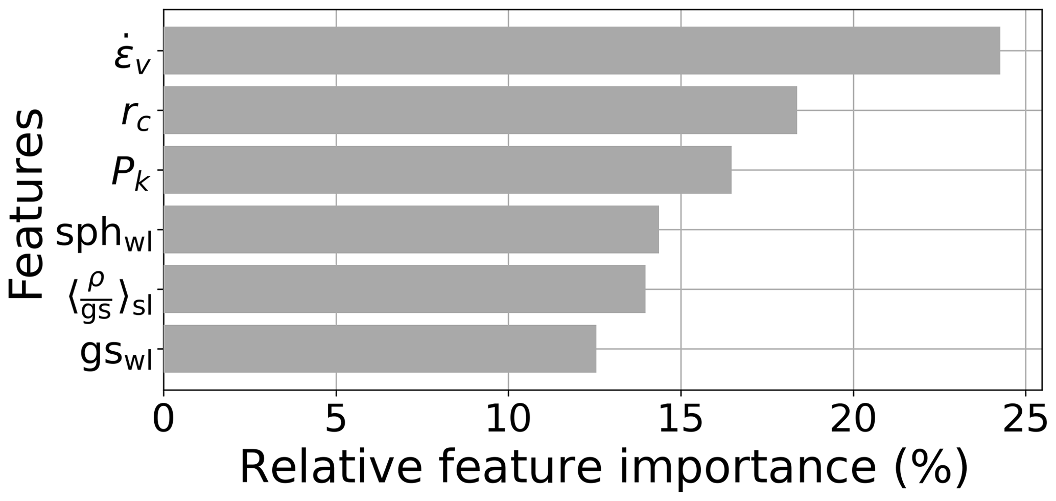
Figure 6 Feature importance ranking for the final model, based on evaluating the Gini impurity decrease at each split for every tree in the RF. The most important features were viscous deformation rate (${\dot{\mathit{ϵ}}}_{\mathrm{v}}$), critical cut length (r_c), skier penetration depth (P_k), sphericity of grains in the weak layer (sph_wl), mean of the ratio of density and grain size of the slab ($\langle \frac{\mathit{\rho }}{\text{gs}}{\rangle }_{\text{sl}}$), and weak layer grain size (gs_wl). For further details on these features, see Appendix B (Table B1).

4.2 Model evaluation

4.2.1 Performance assessment with the SWISS data set

We evaluated the performance of the RF model by classifying the manually defined weak layers for the profiles from the SWISS data set. Using the default classification threshold of 0.5, the overall accuracy was 88 %, 68 of the 75 unstable weak layers were correctly classified (recall of 91 %) and 39 of 46 stable weak layers were classified correctly (specificity of 85 %; Table 1 and Fig. 7b). The precision value was high (91 %) as only 7 of the 75 profiles predicted as unstable were stable according to the ground truth label. Although the classification threshold of 0.5 resulted in good model performance, the optimal threshold value maximizing Youden's J statistic was 0.71 (compare orange and red dots in Fig. 7a). With a threshold of 0.71, precision and specificity scores improved at the expense of the recall value (Table 1). From an operational perspective, it is thus questionable whether the increased number of false negative predictions associated with this Youden index optimization indeed represents an improvement.

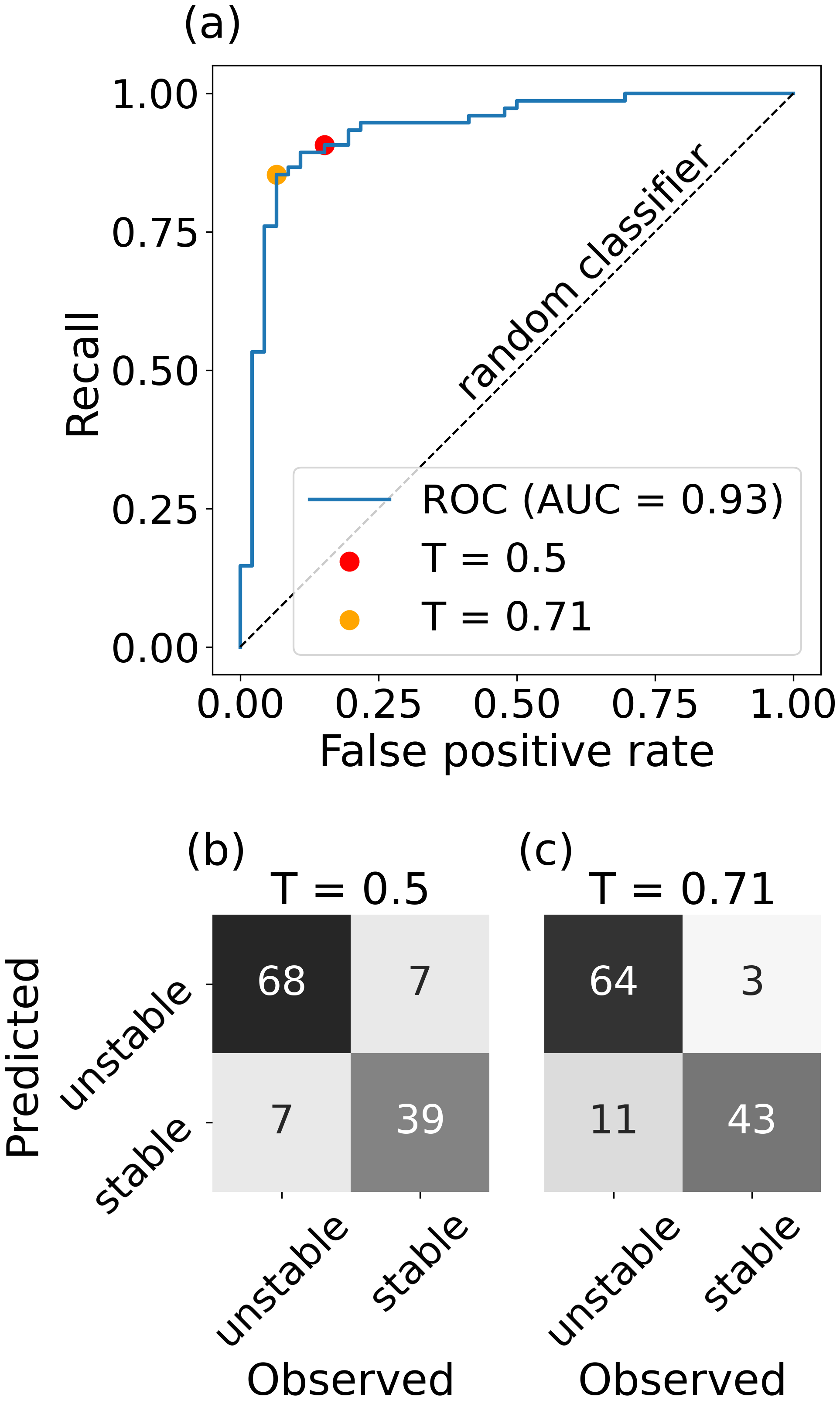
Figure 7 (a) ROC curve analysis and (b, c) contingency tables for the classification of the manually determined weak layers of the SWISS data set. Contingency tables are shown for (b) the default threshold (T=0.5) and (c) the optimized threshold (T=0.71) obtained from the ROC curve analysis.

Table 1 Performance measures for the classification of profiles from the SWISS data set based on the manually determined weak layers and using two different thresholds (T): 0.5 (default) and 0.71 (optimized).

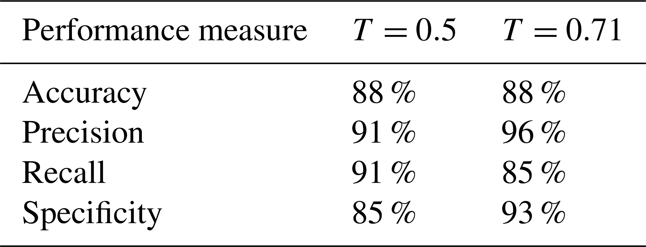
Figure 8 Average values 〈P_unstable〉±σ of the probability of instability over all manually determined weak layers shown for each RB–LN class of (a) the DAV data set and (b) the SWISS data set.

4.2.2 RF model applied to other stability classes

We determined P_unstable (Eq. 8) for all manually selected weak layers from the DAV data set and computed mean values for each RB–LN subgroup (Fig. 8a). P_unstable values decreased from top to bottom, i.e., from higher to lower LN values, and from the left to the right, i.e., from higher to lower RB stability. Considering only the RB stability classes of both data sets not used for training, P_unstable decreased from the marginal RB stability class poor (mean 0.73, 67 % of 119 profiles (DAV 44, SWISS 75) predicted as unstable (i.e., P_unstable ≥ 0.71)) to the marginal RB stability class good (mean 0.45, 29 % of 185 profiles (DAV 139, SWISS 46) predicted as unstable). The decrease was even more pronounced between the subsets with LN ≥ 3 (mean 0.76, 72 % of 169 profiles (DAV 94, SWISS 75) predicted as unstable) compared to LN = 1 (mean 0.31, 14 % of 79 profiles (DAV 33, SWISS 46) predicted as unstable), suggesting that P_unstable of the manually detected weak layers in the simulated profiles correlated more strongly with LN than with the observed stability as assessed with a RB test.

Overall, these results suggest that our RF classifier provides valuable information on snow instability for two reasons. First, weak layers associated with lower stability in terms of the RB class had higher values of P_unstable. Second, higher LN values increase the likelihood that the associated simulated profile indeed exhibits unstable properties, which was also reflected in higher P_unstable values. Note that both observations and simulations contain uncertainties that are difficult to quantify. This is reflected in relatively high values of the standard deviations of P_unstable, typically in the range of 20 %–30 %.

Figure 9 Three profile pairs from the DAV data set with (a, c, e) manually observed snow profiles and (b, d, f) corresponding simulated snow stratigraphy obtained with SNOWPACK. Hand hardness and grain type (colors) were coded after Fierz et al. (2009) (for further explanation see caption of Fig. 3). The dashed horizontal line in the manual profile displays the observed height of the RB failure layer, and the corresponding manually determined layer is indicated by a dashed line in the respective simulated profile. The black line in the simulated profiles shows the probability of instability P_unstable determined for each layer. Observed RB results were (a) RB score 2, whole block; (b) RB score 6, edge; and (c) RB score 4, partial. The local danger level estimates were (a) LN=3, (b) LN=2 and (c) LN=1.

4.2.3 RF model applied to complete snow profiles

Figure 9 shows P_unstable calculated for all layers in three example profiles (black line, right-hand side of subplots), except for the uppermost layer as it has no overlying slab. These examples indicate that typical weak layers, such as depth hoar, surface hoar or soft faceted layers, yield higher P_unstable values than layers consisting of rounded grains, melt–freeze crusts and harder layers of facets. Indeed, the mean P_unstable value for all layers of persistent grain types with hand hardness ≤ 2 (four fingers) in both data sets was 0.37 ± 0.3, while for layers consisting of rounded grains or melt–freeze crusts it was 0.17 ± 0.17. The high standard deviation for the layers of persistent grain types suggests that the stability is determined not only by layer properties but also by the overlying slab. New snow layers (i.e., precipitation or defragmented particles) had the highest average values of P_unstable (0.52 ± 0.26). We further observed simulated layers with high P_unstable values, i.e., potential weak layers, not observed in the manual counterpart (e.g., Fig. 9c and d – surface hoar present in simulated but not in manual profile).

To explore if the maximum value of P_unstable can be used to describe the stability when the weak layer is not known, we determined P_max=max(P_unstable) for each profile of the SWISS data set. Using P_max and a default threshold of 0.5, we classified the profiles as unstable and stable. The resulting contingency table is shown in Fig. 10b, and the associated performance measures are shown in Table 2. With this threshold value, the classifier performed well in labeling unstable profiles as unstable (recall 96 %), but almost half of the stable profiles were misclassified (specificity 55 %). The optimal threshold value for P_max was 0.77 (orange dot in Fig. 10c), greatly improving the overall performance (third column in Table 2, all performance measures > 90 %). This optimal threshold value of 0.77 was close to the optimized value obtained for the classification of the manually selected weak layers (i.e., 0.71, Sect. 4.2.1), which led to similar values of the performance measures (second column in Table 2).

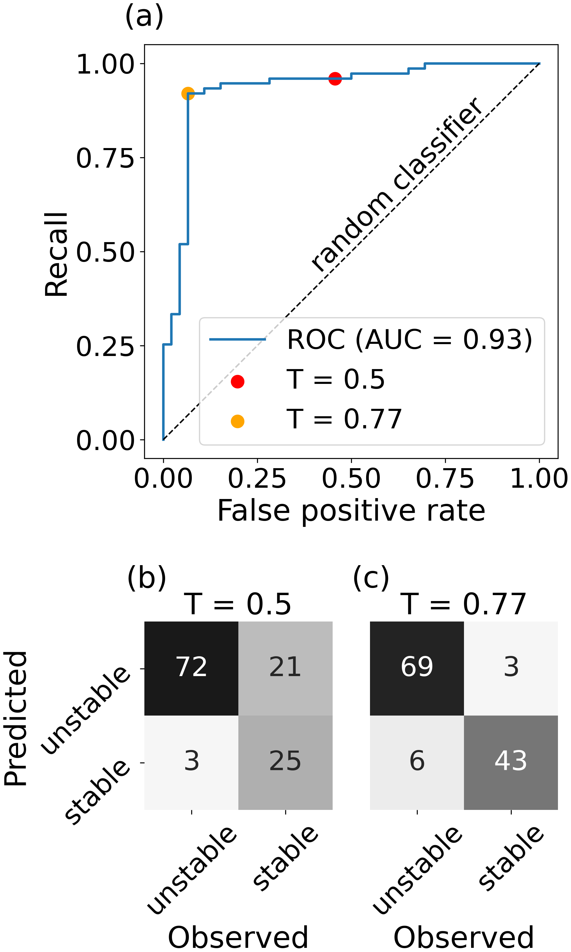
Figure 10 (a) ROC curve analysis and (b, c) contingency tables for the classification of the unstable and stable classes from the SWISS data set, using the maximum value of the probability of instability, P_max. Contingency tables are shown for (b) the default threshold (T=0.5, red dot in a) and (c) the optimized threshold (T=0.77, orange dot in a) obtained from the ROC curve analysis.

Table 2 Performance measures for the classification of profiles from the SWISS data set based on the maximum value of the probability of instability (P_max) for different classification thresholds (T): 0.5 (default), 0.71 (optimized value for the classification of manually selected weak layers) and 0.77 (optimized value for the classification based on P_max).

4.2.4 Weak layer detection

To investigate if our RF model can be used to detect the weakest layer within a profile, we calculated the probability of detecting the manually picked weak layers with the local maxima of P_unstable as described in Sect. 3.2.2 (point 3). For the DAV data set, the overall POD was 60 %, and POD values strongly varied between different RB–LN classes (Fig. 11a). While for the unstable training class, the POD was high (86 %), the POD was low (37 %) for the stable training class. For the SWISS data set, the POD was 75 % for the unstable class and 46 % for the stable class (Fig. 11b). Lower POD values for classes with higher stability can be explained by the fact that the manual identification of the simulated layer associated with the RB failure layer was generally less clear, since a prominent weak layer was often not present. In addition, “weak” layers, which only failed with a large additional load (high RB score) and which result in a fracture not propagating (a partial RB failure), are usually not associated with instability (Schweizer and Jamieson, 2003). Thus, it seems plausible that distinguishing these (not truly) weak layers from other layers within a profile is more difficult; yet it is also likely to be less relevant.

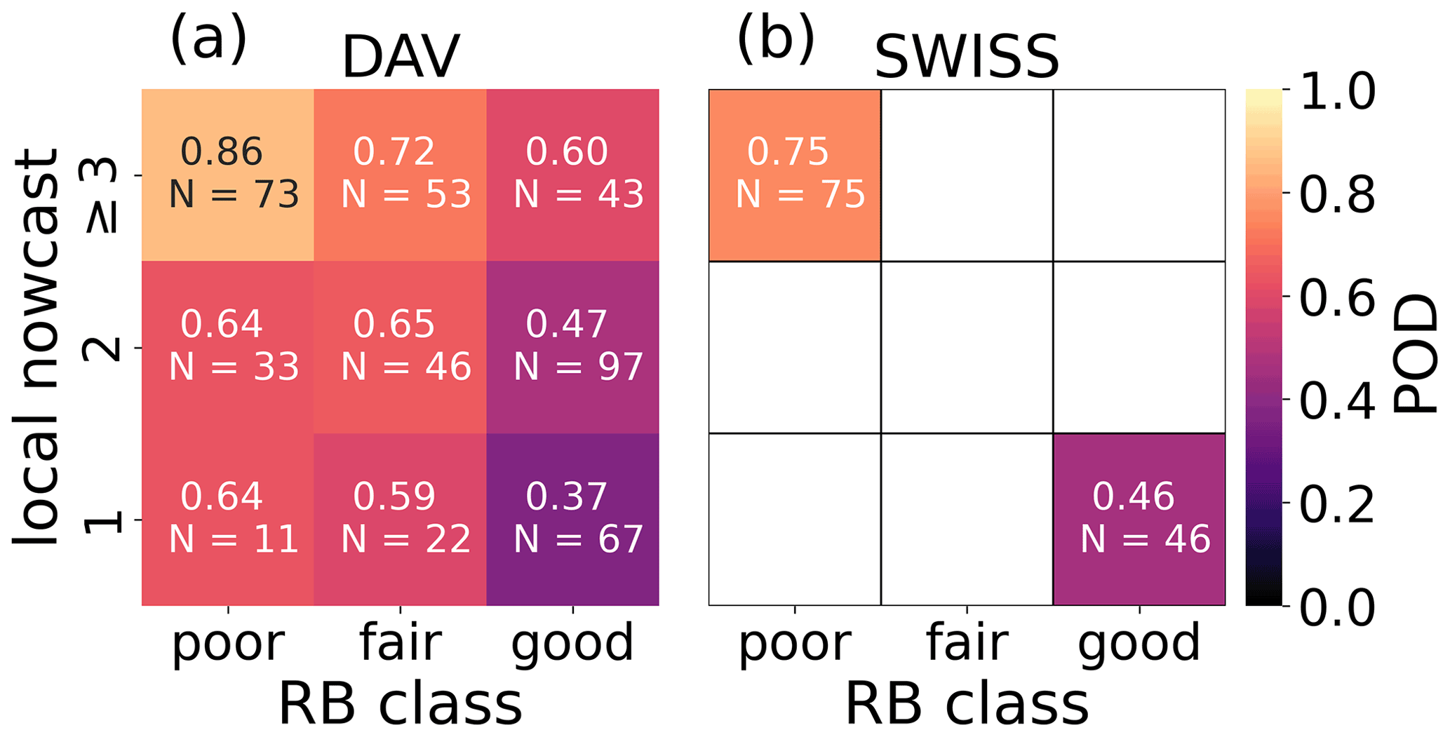
Figure 11 Probability of detecting the weakest layer with the three largest local maxima of P_unstable and adjacent layers within 3 cm of these local maxima shown for every RB–LN class of (a) the DAV and (b) the SWISS data set.

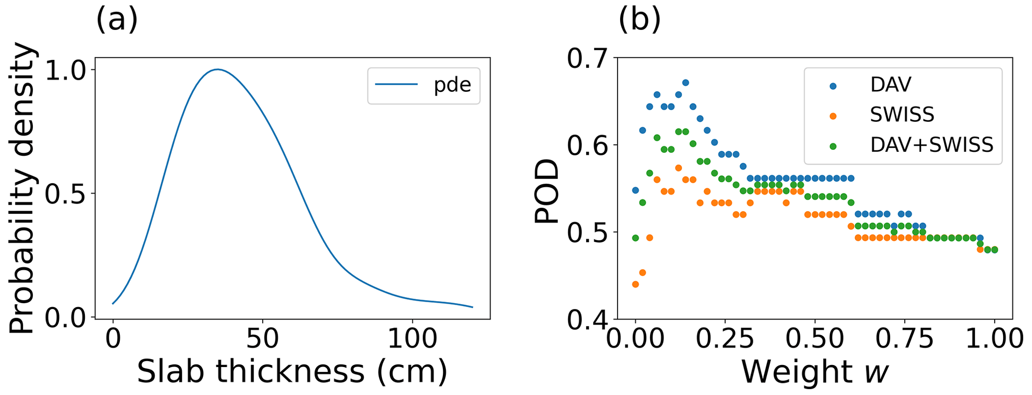
Figure 12 (a) Normalized Gaussian kernel density estimate (pde) for the distribution of observed slab thicknesses in the unstable class of the DAV data set. (b) Probability of detecting the manually picked weak layer in dependence on the weighting factor w used in the calculation of $P_{\text{unstable}}^{\ast }\left(w\right)$ (Eq. 9) for the unstable classes in the DAV data set (blue markers), in the SWISS data set (orange markers) and in the combination of both (green markers).

Our RF model does not contain any feature explicitly describing slab thickness. However, it is well known that weak layers associated with skier-triggered avalanches are typically within the first meter from the snow surface (e.g., Schweizer and Camponovo, 2001; van Herwijnen and Jamieson, 2007). To account for this, we investigated if adding information on slab thickness improved the weak layer detection by defining the function

$$\begin{array}{}\text{(9)}& P_{\text{unstable}}^{\ast }\left(w\right)=P_{\text{unstable}}\left[(\mathrm{1}-w)+w\cdot {\displaystyle \frac{\text{pde}\left(D_{\text{slab}}\right)}{{\text{pde}}_{\text{max}}}}\right],\end{array}$$

which includes a weighting factor w and the normalized estimated probability density function pde(D_slab) of the observed slab thicknesses D_slab in the DAV data set (Fig. 12a). We analyzed the influence of the weighting factor w on the probability of detecting the manually determined weak layer with the maximum value $P_{\text{max}}^{\ast }\left(w\right)=\text{max}\left(P_{\text{unstable}}^{\ast }\right(w\left)\right)$. We counted a weak layer as detected when $P_{\text{max}}^{\ast }\left(w\right)$ was located within 3 cm of the manually picked weak layer. To calculate the POD, we only considered the unstable classes of the DAV and SWISS data sets. For w=0, i.e., when not accounting for slab thickness, the POD was 55 % for the DAV data set and 44 % for the SWISS data set. The largest POD values of 67 % (DAV data set) and 57 % (SWISS data set) were achieved for weights of w=0.14 and w=0.12, respectively. For larger weighting factors, the POD decreased again (Fig. 12b). Thus, accounting for slab thickness increased the probability of detecting a weak layer found with a RB test and hence a weak layer which can potentially be triggered by a human. On the other hand, the relatively low values of w for the highest POD values suggest that with our model, accounting for slab thickness is of only limited importance.

4.2.5 Comparison with avalanche activity

To demonstrate the practical applicability, we applied the RF model to SNOWPACK simulations for five winter seasons (2014/15 to 2018/19) driven with meteorological data from the AWS at the Weissfluhjoch study site at 2540 $\mathrm{m}\mathrm{a}.\mathrm{s}.\mathrm{l}.$ For these five winter seasons (597 d), values of P_max were significantly higher on avalanche days (median 0.88) than on non-avalanche days (median 0.51; Mann–Whitney U test, p<0.001; Fig. 13). Applying the threshold value of 0.77 to the daily values of P_max yielded an overall accuracy of 73 % for discriminating avalanche days from non-avalanche days. Of the 252 avalanche days, 69 % occurred on days when the threshold was exceeded, while for 75 % of the 345 non-avalanche days, P_max was below the threshold.

Figure 13 Distribution of maximal values P_max of the probability of instability P_unstable calculated for the simulated snow stratigraphy at the location of the AWS Weissfluhjoch (WFJ, 2540 $\mathrm{m}\mathrm{a}.\mathrm{s}.\mathrm{l}.$) on avalanche days and non-avalanche days during the winter seasons 2014/15 to 2018/19. Avalanche days were defined as days with at least one recorded dry-snow avalanche in the region of Davos which was greater than avalanche size class one, released naturally, was human-triggered or had an unknown trigger type. Boxes show the interquartile range from the first to third quartiles, and the horizontal line displays the median. The upper and lower whiskers mark 1.5 times the interquartile range above the third and below the first quartiles, respectively. The dashed line displays the classification threshold T=0.77. Number of avalanche days: N=252; number of non-avalanche days: N=345.

Two examples for the temporal evolution of the simulated snow stratigraphy in terms of grain types and values of P_unstable and P_max over entire winter seasons at the WFJ are shown in Figs. 14 (winter 2016/17) and 15 (winter 2017/18) in comparison to the avalanche activity index (AAI) of observed avalanches in the region of Davos. The 2016/17 winter season was characterized by below-average snow depth and the presence of three prominent persistent weak layers throughout the season (dark-blue layers in Fig. 14c). The daily P_max was often in the vicinity of these persistent weak layers (black line in Fig. 14c). Three larger precipitation events in early January, early February and mid-March were associated with increased avalanche activity (blue bars in Fig. 14b). These periods of increased avalanche activity all occurred when P_max values exceeded the threshold value of 0.77 (yellow-shaded regions in Fig. 14b). The 2017/18 winter season was characterized by above-average snow depth and a lack of persistent weak layers. P_max was generally located below the recent new snow (black line in Fig. 15c). Three large snowfall events between December and the middle of January resulted in three distinct avalanche periods, all of which corresponded to P_max values exceeding the threshold value of 0.77 (yellow-shaded regions in Fig. 15b). Overall, this qualitative comparison suggests that applying the RF model to complete snow profiles provides valuable information linked to regional avalanche activity.

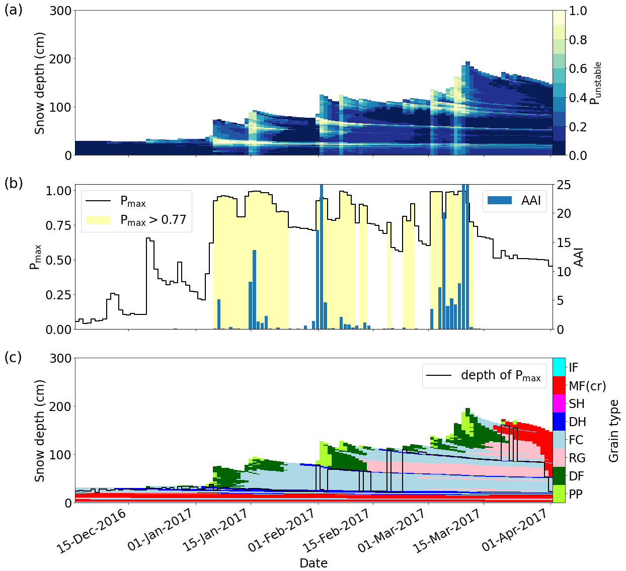
Figure 14 Evolution of (a) probability of instability P_unstable (colors), (b) maximal values P_max (black line) and avalanche activity index (AAI, blue bars), and (c) the depth of P_max (black line) and grain types (colors) calculated for the simulated snow stratigraphy at the AWS Weissfluhjoch (WFJ, 2540 $\mathrm{m}\mathrm{a}.\mathrm{s}.\mathrm{l}.$) during the winter season 2016/17. Grain types were coded after Fierz et al. (2009) (see caption of Fig. 3). Yellow-shaded areas in (b) indicate days with P_max exceeding the threshold T=0.77.

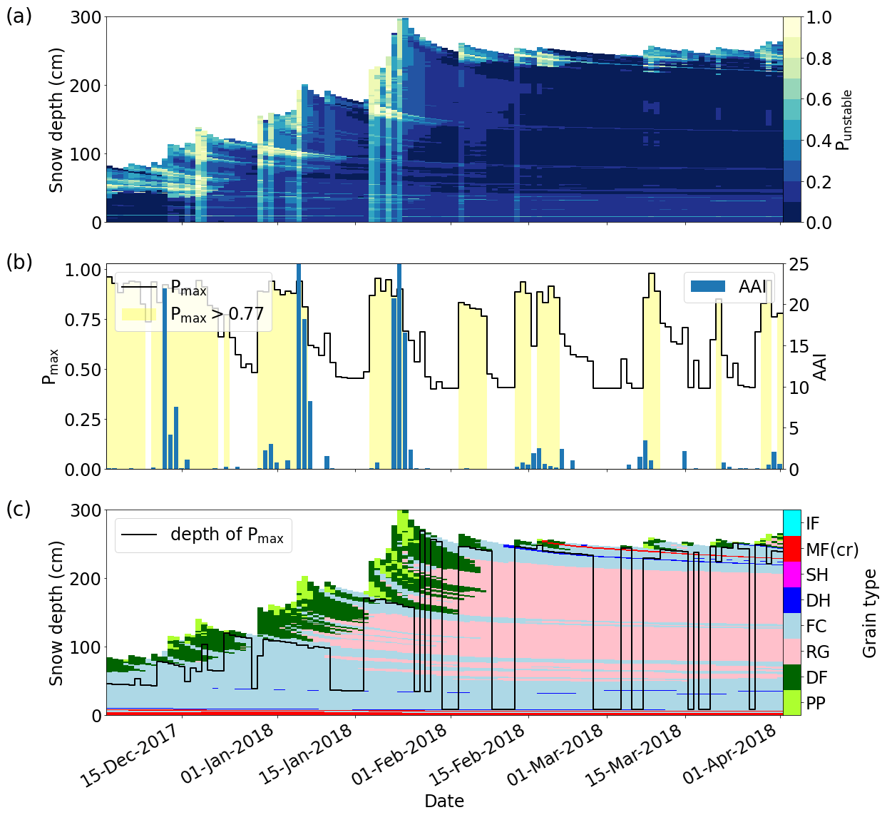
Figure 15 Evolution of (a) probability of instability P_unstable (colors), (b) maximal values P_max (black line) and avalanche activity index (AAI, blue bars), and (c) the depth of P_max (black line) and grain types (colors) calculated for the simulated snow stratigraphy at the AWS Weissfluhjoch (WFJ, 2540 $\mathrm{m}\mathrm{a}.\mathrm{s}.\mathrm{l}.$) during the winter season 2017/18. Yellow-shaded areas in (b) indicate days with P_max exceeding the threshold T=0.77.

5 Discussion

We trained a RF classifier to distinguish between unstable and stable snow profiles simulated with the snow cover model SNOWPACK. The resulting model provides a probability of instability for every single layer of a snow profile using six features describing the layer and the overlying slab. To train and validate the model, we relied on data from manual snow profiles with RB tests and compared the results from our model to avalanche activity in the region of Davos.

5.1 Data

A critical component for the construction of the RF model was a data set linking observed and modeled snow instability. We therefore performed a one-to-one comparison of 742 pairs of observed and simulated snow profiles. The snow cover simulations relied on interpolated meteorological data or measurements from an AWS in the vicinity of the manual profile projected to virtual slopes which do not account for the influence of the surrounding terrain. Thus, the simulations cannot be expected to reproduce the exact observed snow stratigraphy. In particular, manual snow profiles are preferentially recorded at locations expected to exhibit poor stability (targeted sampling), e.g., slopes with below-average snow depth (McClung, 2002; Techel et al., 2020a). By scaling the precipitation input (Sect. 2.3), we intended to align modeled and observed snow depths. However, this scaling method mimics local snow redistribution on a very basic level only and cannot replace the application of high-resolution wind fields required to explicitly simulate snow drift. While of the DAV profile pairs, only 13 % did not meet the predefined similarity criteria, 47 % of the SWISS profiles were excluded, indicating that the interpolation of meteorological data from several stations to the profile location led to a better representation of the local snow stratigraphy than merely simulating the snowpack at a single nearby AWS. Our approach of comparing profiles was based on the manual selection of a simulated layer corresponding to the observed RB failure layer and thus contained a certain degree of subjectivity. Recently developed automated methods for profile comparison (Viallon-Galinier et al., 2020; Herla et al., 2021) are less time-consuming and may provide a more objective alternative for profile comparisons in future studies.

5.2 Target variable

As with any classification task, the definition of a suitable target variable was crucial. In the field, instability is evaluated using a stability test, such as the RB test. We combined the observed RB test result from the manual profiles with an estimate of avalanche danger (local nowcast) to build a binary target variable describing stability at both ends of the stability spectrum (stable vs. unstable, Table 2). While past studies (Gaume and Reuter, 2017; Monti et al., 2014) used only observed stability test results to train or evaluate snow instability models, exclusively relying on the observed RB test result as the target variable was not sufficient in our case. In the mentioned studies, either only observed data were considered or the stability test was conducted next to the AWS where the simulation was run. In our study, however, we used interpolated meteorological data. Due to the reasons described in Sect. 5.1, the simulated properties of the snow profiles, which yielded the explanatory variables for the classification task, thus cannot fully capture the peculiarities of the snowpack at the observation site. By considering the local nowcast assessment of avalanche danger as an additional criterion, we selected those profiles that were likely to represent either rather stable or rather unstable conditions. As illustrated in various studies (e.g., Techel et al., 2020b; Schweizer et al., 2021b), the proportion of poor stability test results increases with the local danger level. Consequently, a profile with poor stability can be assumed to be more representative of the conditions at considerable danger level (level 3) and consequently to be better captured by the SNOWPACK simulation compared to a poor stability test result obtained at low danger level (level 1).

5.3 Explanatory variables

We reduced the explanatory input variables of our RF model to six features while maintaining a high classification performance. Two features, the critical cut length and viscous deformation rate, combine slab and weak layer properties; two features are related to microstructural weak layer properties (grain size and sphericity); one feature describes snow surface and upper slab conditions (skier penetration depth); and one feature relates to bulk slab properties (mean of the ratio of density and grain size of all slab layers). The combination of these parameters and the relationship between target response and individual input features depicted by the PD plots (Appendix B, Fig. B2) fit well with our conceptual understanding of snow instability.

The viscous deformation rate was the most important feature in our model (Fig. 6). It is proportional to the normal stress of the slab and inversely proportional to the viscosity (Appendix B, Table B1). High viscous deformation rates can thus occur during loading (i.e., snowfall) and in particular in layers with low viscosity, such as layers composed of low-density new snow. In our training data set, viscous deformation rates were significantly higher for unstable than for stable layers (Mann–Whitney U test, p<0.001).

In the context of human-triggered avalanches, the importance of skier penetration depth is well established (e.g., Schweizer and Camponovo, 2001; Jamieson and Johnston, 1998). Large penetration depths increase the stress exerted on potential weak layers in the snowpack and thereby facilitate skier triggering. Schirmer et al. (2010) found skier penetration depth to be the most important variable to classify simulated snow profiles as unstable using a single classification tree model. The parameterization of the skier penetration depth in SNOWPACK is inversely related to the mean density of the upper 30 cm of the snow cover and thus relates to slab properties (Schweizer et al., 2006). Changes in the penetration depth are therefore closely linked to the presence of new snow. In our RF model, a second feature characterizing the slab was the mean ratio of density and grain size of all slab layers. We assume that this parameter was important as it can distinguish cohesionless slabs (low-density new snow consisting of large grains) from well-bonded slabs (higher density consisting of small rounded grains) typically associated with slab avalanches.

The importance of the critical cut length r_c in our RF model is in line with a recent study by Richter et al. (2019), who observed that minimal values in modeled critical cut length often coincided with observed persistent weak layers. As such, it is likely that the critical cut length favors the classification of persistent weak layers as unstable. While the critical cut length is related to crack propagation, our set of features did not include any parameter related to failure initiation. Indeed, the traditional skier stability index SK₃₈ (Föhn, 1987b; Jamieson and Johnston, 1998; Monti et al., 2016) and the related failure initiation criterion (Reuter et al., 2015a) had lower feature importance scores (Appendix B, Fig. B1). Recently, Reuter et al. (2022) suggested using a combination of the critical cut length and a failure initiation index to differentiate stable from unstable profiles using a threshold-based approach. Applying these thresholds without further training to our DAV data set resulted in a recall of 42 %. Training a decision tree of depth two with the same features on the DAV data set yielded a 5-fold cross-validated accuracy of 68 %; the accuracy was however higher (72 %) when using only the critical cut length as input feature. While this suggests that the strength-over-stress initiation criteria do not provide any added value compared to the critical cut length, we cannot exclude the possibility that these results are biased by uncertainties introduced by the manual identification of the weak layers in the SNOWPACK simulations.

5.4 Training and evaluating the RF model

To train the RF model, we used the DAV data set with detailed snow cover and stability observations (Schweizer et al., 2021b), as well as high-quality meteorological input for SNOWPACK from a dense network of AWSs. Nevertheless, the number of profile pairs in the stable and unstable classes was rather small (N=67 and N=73, respectively). Due to this limited number of data points, we conducted feature selection, hyperparameter optimization and training of the RF model all on the same data set without further splitting. This resulted in a 5-fold cross-validated accuracy of 88 % on the balanced DAV training data. Schirmer et al. (2010) achieved a cross-validated accuracy of 75 % when training a classification tree to distinguish between rather stable and rather unstable simulated profiles. However, their definition of the target variable differed from ours and their data set was imbalanced.

The validation of our model on a second independent data set (SWISS) revealed a robust performance (overall accuracy 88 %) in the binary classification of the manually determined weak layers. Optimal performance with respect to Youden's J statistic was reached with a classification threshold of 0.71, although the default threshold of 0.5 used in the training configuration led to the same overall accuracy. For any application of the model, the threshold should hence be adjusted according to the specific requirements regarding detection and false alarm rate. To overcome the subjectivity inherent in the manual identification of weak layers in the simulated profiles, we again classified the SWISS profiles using P_max. With an optimized classification threshold (0.77), this classification yielded an accuracy of 93 %. Using P_max thus led to a better classification performance than using the P_unstable value of the manually selected weak layers. The high optimal threshold value of 0.77 could be due to the fact that some weaker layers in the simulations were not present in the manual profiles. Furthermore, this shift in threshold values might also be related to differences between the training and validation data set. The profiles used for training were all observed in the region of Davos, an area characterized by an inner-alpine snow climate (e.g., Schweizer et al., 2021b). While for 80 % of the manual profiles in the training data set, the RB failure interface was adjacent to a layer including persistent grain types, this was the case for only 57 % of the profiles in the validation data set, which were conducted in various snow climatological regions of the Swiss Alps.

5.5 Model strengths and limitations

Applying our RF model to snow layers not falling into the stability categories of the binary target variable produced reasonable results (Figs. 8 and 9). Moreover, the detection of weak layers performed well under poor stability conditions (Fig. 11). While previous studies (Schweizer et al., 2006; Schirmer et al., 2010) used separate routines for weak layer detection and instability assessment, our approach can assess instability and detect the weakest layer with one single index, the maximum of the probability of instability over all layers of the simulated snow profile.

Clearly, the interpretability of our RF model is constrained by its black-box character. However, an advantage of RF models is the ability to capture complex multi-variable relationships between features and the target variable, beyond linear or threshold-based dependencies. Moreover, our model is built on only six features, which facilitates its application. An apparent limitation of our method is the lack of profiles with intermediate stability in the training data, which prevents a direct interpretation of the absolute values of the probability of instability. The probability of instability does not directly refer to a physical quantity but should always be interpreted as a mean vote of trees trained with profiles from both ends of the stability spectrum. Setting thresholds to differentiate fair from poor or good stability would require more training data. Nonetheless, the comparison of modeled snow instability at the WFJ with observed regional avalanche activity revealed the potential of our model to indicate conditions of poor stability by using the optimized threshold value from the binary classification. The model chain captured the major avalanche cycles of the two winter seasons shown in Figs. 14 and 15 and discriminated reasonably well between avalanche and non-avalanche days (recall 69 %, specificity 75 %) despite a lack of information on spatial snow distribution in the modeled data as well as potential incompleteness or bias of the observed avalanche data. The transferability of our RF model and its optimized threshold to other snow climatological settings should be evaluated on further independent data sets.

6 Conclusion and outlook

We introduced a novel method to assess dry-snow instability from simulated snow stratigraphy. Our random forest (RF) model provides a probability of instability P_unstable for each layer of a snow profile simulated with SNOWPACK, given six input variables describing microstructural, macroscopic and mechanical properties of the particular layer and the overlying slab. The probability of instability allows the detection of the weakest layer of a snow profile and assessing its degree of instability with one single index, a main advantage of this new model. Although the RF model was trained with only 146 layers manually labeled as either unstable or stable, it classified profiles from an independent validation data set with high reliability (accuracy 88 %, precision 96 %, recall 85 %) using manually predefined weak layers and an optimized classification threshold. The binary classification performance with an optimized threshold was even higher (accuracy 93 %, precision 96 %, recall 92 %) when the weakest layers of the profiles were not known and were instead identified with the maximum of P_unstable. Finally, we illustrated the potential of our model and its optimized threshold value to indicate conditions of poor stability by comparing the temporal evolution of modeled snow instability with observed avalanche activity in the region of Davos for five winter seasons.

With the maximum of P_unstable, our model, in principal, provides an estimate of dry-snow instability for any simulated snow profile for which the required input variables are available. For the derivation of further threshold values which detect intermediate stability, more data are required. The threshold that distinguishes rather unstable from rather stable profiles may need to be adjusted if the simulated stratigraphy originates from models other than SNOWPACK or if applied in a region with a snow climate strongly differing from the conditions in the Swiss Alps.

In the future, the RF model may be used to estimate avalanche danger from simulated snow stratigraphy. To this end, the RF model would be applied to modeled snow stratigraphy at different locations within one region. The respective maxima of P_unstable and the corresponding frequency distribution may then yield information on the snowpack stability as well as the spatial distribution of stability, and the depths of the weakest layers determined with these maxima may provide an indicator of the expected avalanche size. Since this application of the RF model covers all three factors contributing to avalanche hazard (Techel et al., 2020a), it could be of great value for operational avalanche forecasting. This application may even be extended by extracting the grain type of the weak layer to distinguish between the avalanche problem types “persistent weak layer problem” and “new snow problem” (EAWS, 2021). Besides this operational use, the method described is also suited for analyzing past and future changes in snow instability due to climate warming.

Appendix A: Data

The locations of snow profiles and AWSs are shown in Figs. A1 and A2.

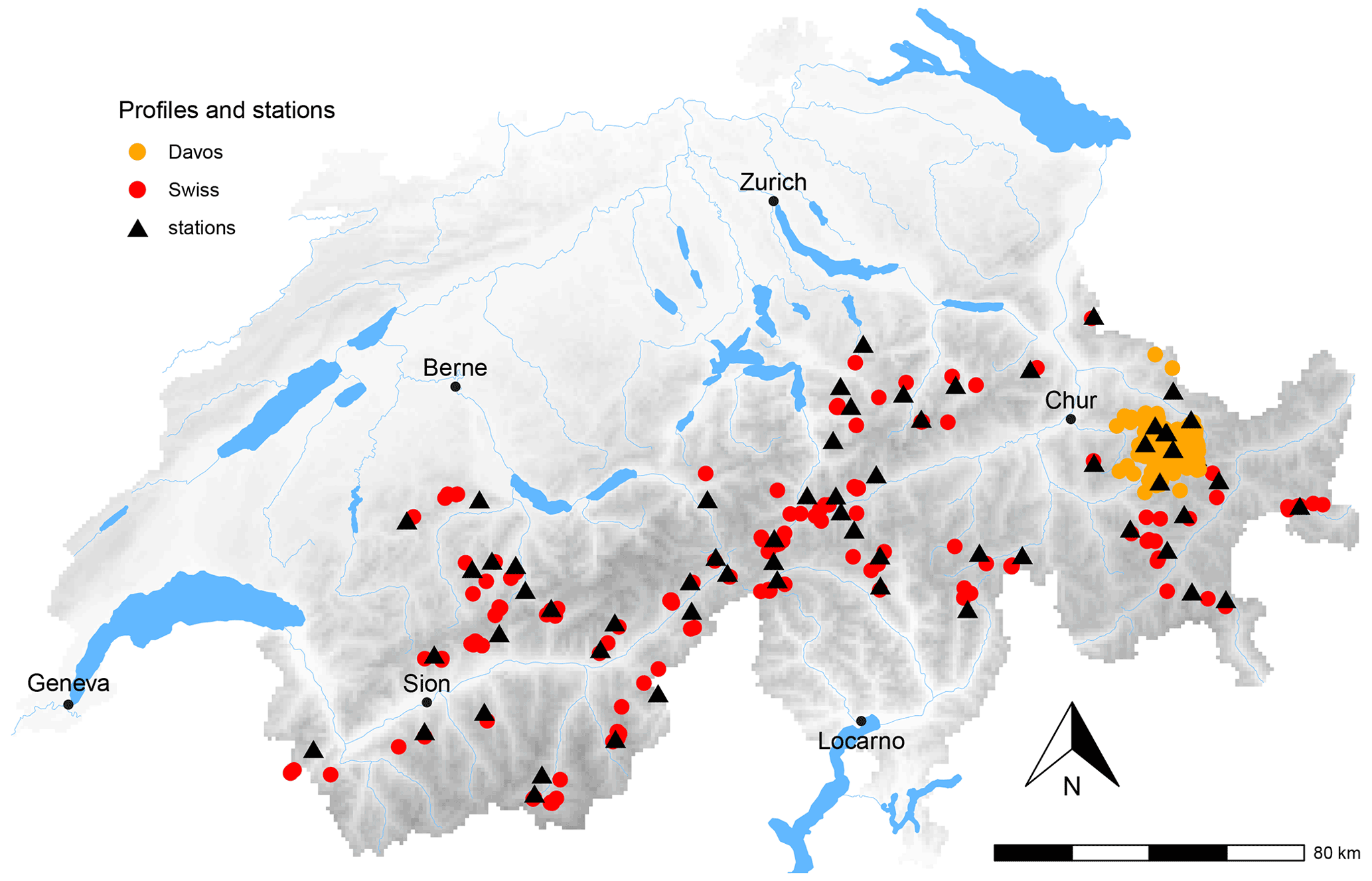
Figure A1 Map of Switzerland showing the locations of the snow profiles and the automatic weather stations used in the Davos and Swiss data set (orange and red markers, respectively). An enlargement of the Davos region is shown in Fig. A2.

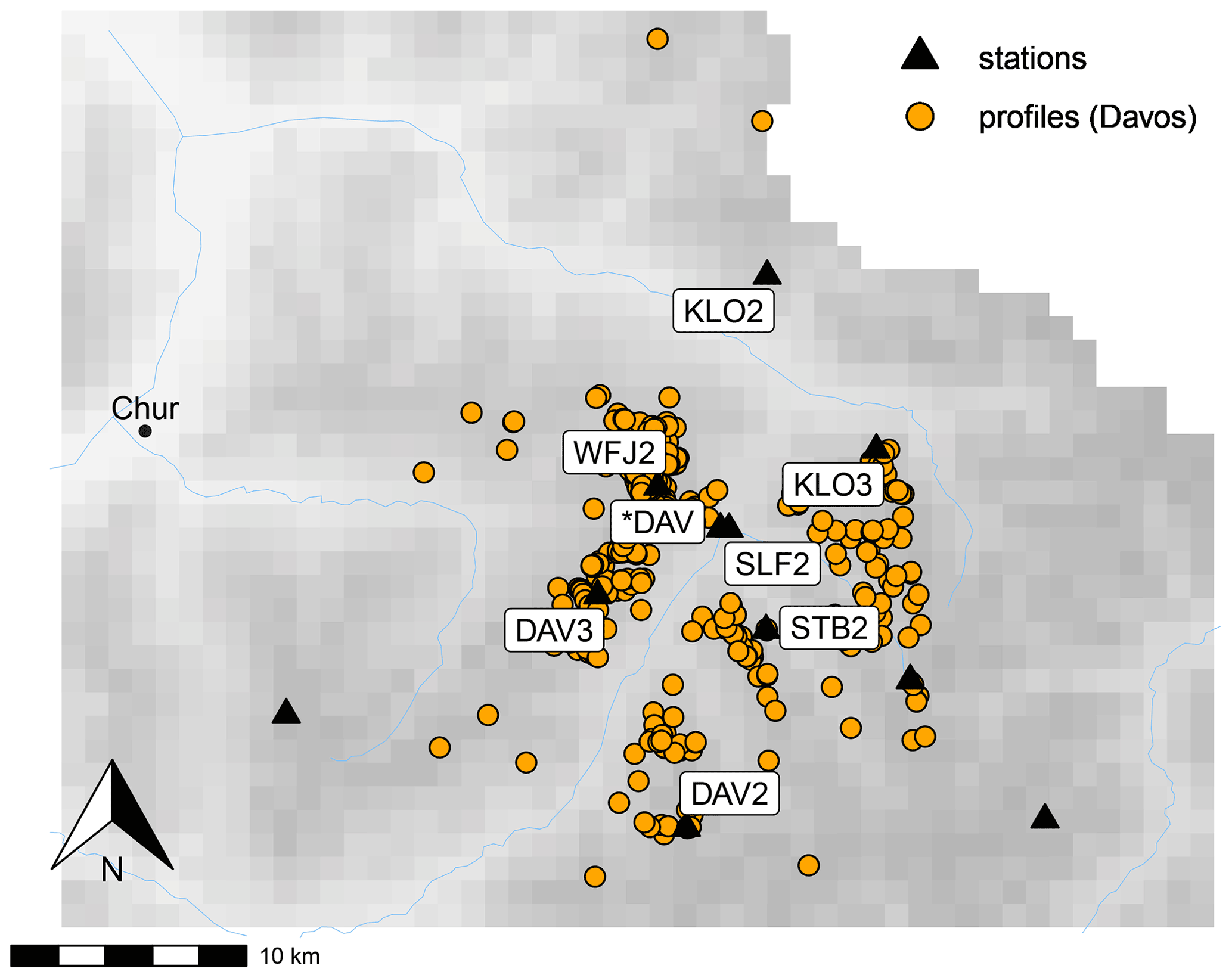
Figure A2 Map showing the region of Davos with the automatic weather stations (with their labels) and the profile locations (orange markers).

Appendix B: Classification model

To build the classification model, we used 34 features which are described in Table B1. The relative importance of a subset of 20 of these features is shown in Fig. B1. The final values of the hyperparameters in the RF model are compiled in Table B2.

Lehning et al. (2002b)Lehning et al. (2002b)Lehning et al. (2002b)Lehning et al. (2002b)Lehning et al. (2002b)Bartelt and Lehning (2002)Lehning et al. (2002b)Jamieson and Johnston (1998)Schweizer et al. (2006)Schweizer and Jamieson (2007)Schweizer and Jamieson (2007)Monti et al. (2014)Jamieson and Johnston (1998)Bartelt and Lehning (2002)Jamieson and Johnston (1998)Monti et al. (2016)Föhn (1987b)Jamieson and Johnston (1998)Monti et al. (2016)Reuter et al. (2015a)Richter et al. (2019)Lehning et al. (2002b)Lehning et al. (2002b)Bartelt and Lehning (2002)Lehning et al. (2004)

Table B1 Table with all features describing slab (sl) and weak layer (wl) properties.

Figure B1 Feature importance after hyperparameter optimization round 1.

Table B2 Hyperparameters of final random forest model.

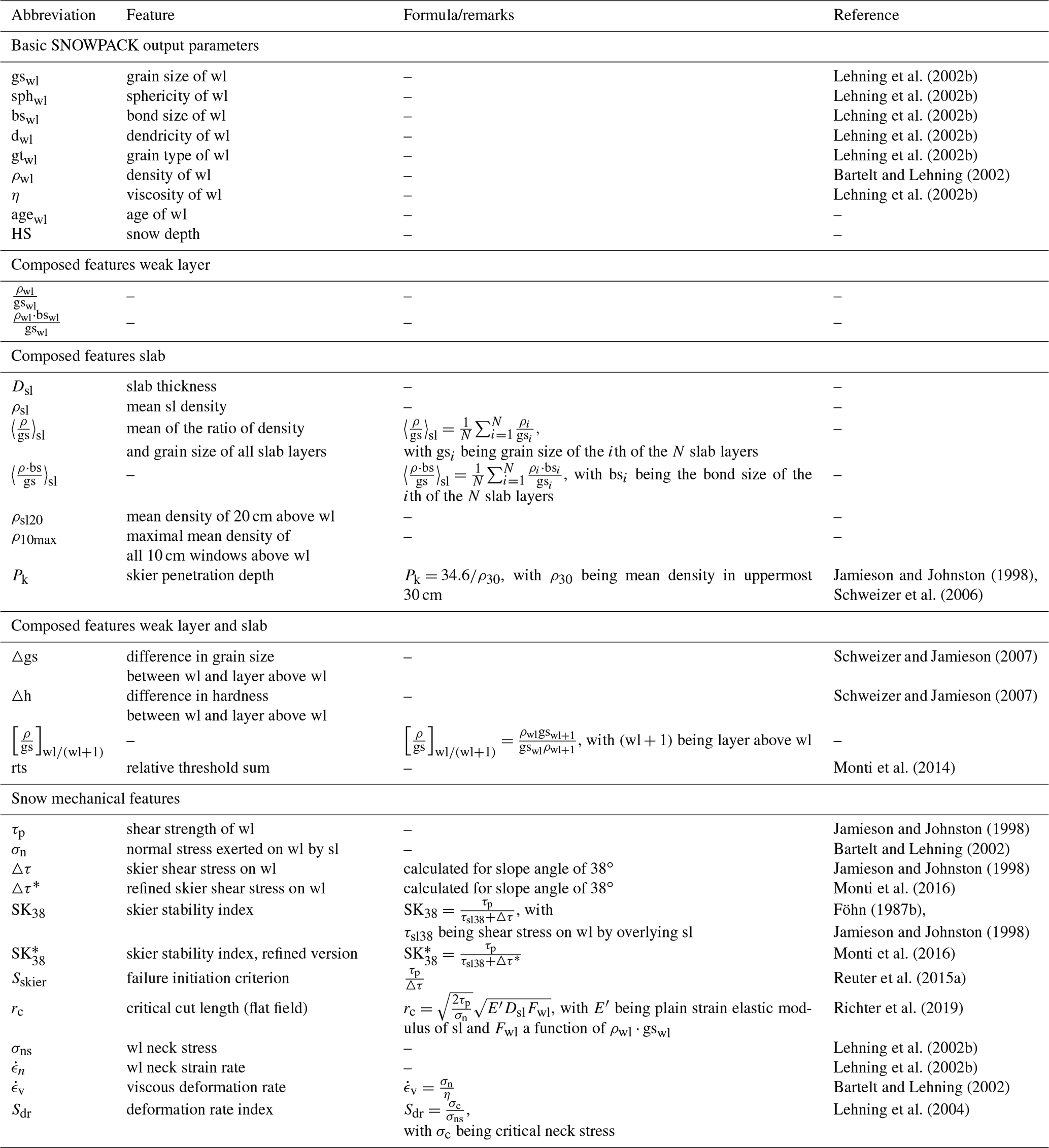
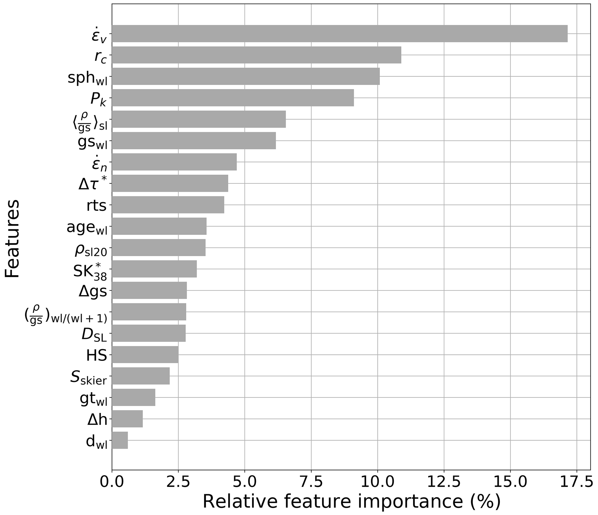
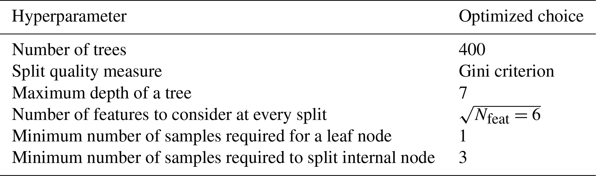
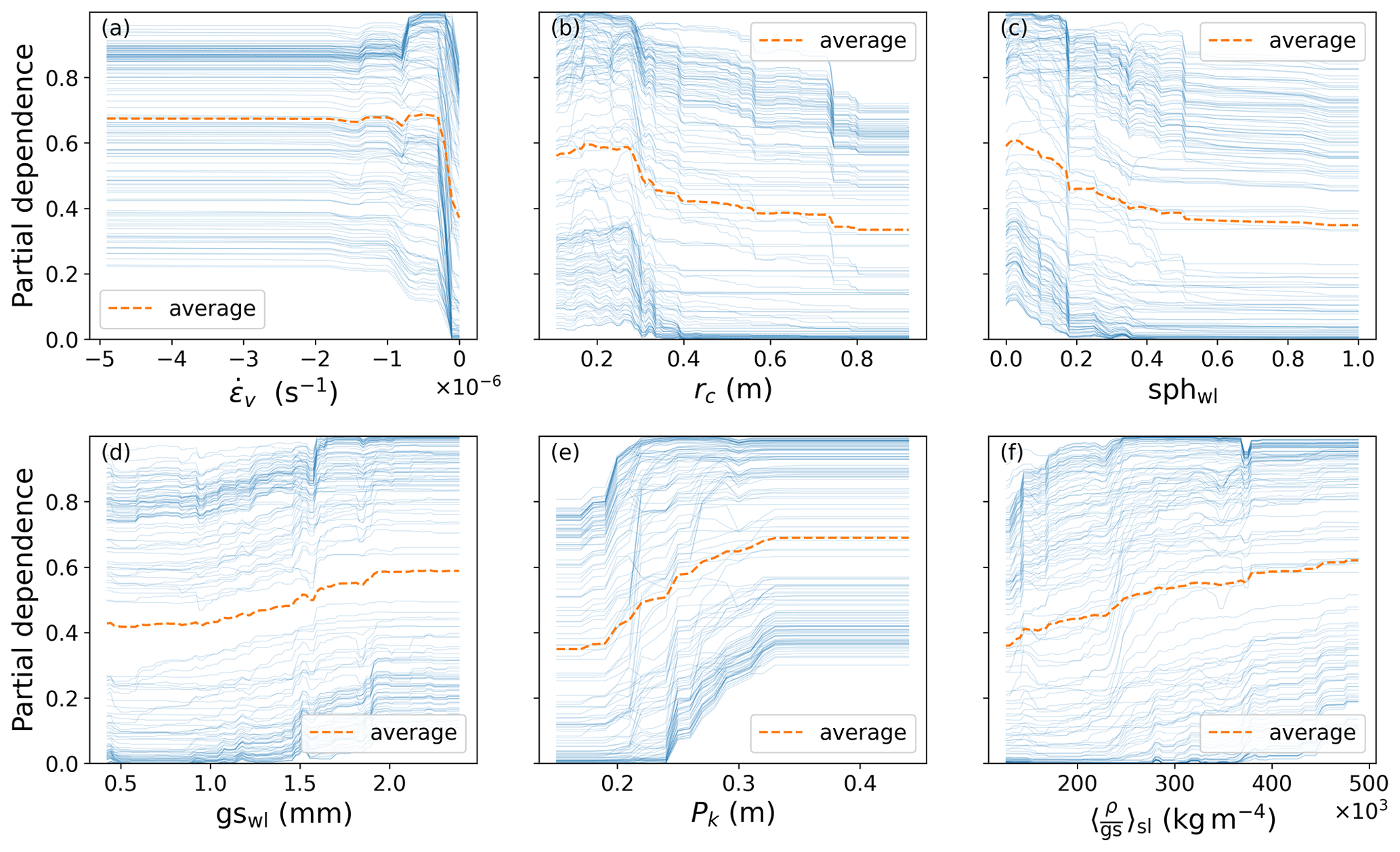
Figure B2 Partial dependence (PD) plots showing the relationship between target response and individual input features (a viscous deformation rate, b critical cut length, c sphericity of the weak layer, d grain size of the weak layer, e skier penetration depth, f mean of the ratio of density and grain size of the slab). Each plot depicts how a given feature influences the predicted outcome when marginalizing over the distributions of all other features. The values for each PD plot were computed by applying the RF model to all data points of the training data set and then varying the value of the feature of interest while keeping the values of all other features fixed. The blue lines show the target response for the individual samples, and the orange line displays the mean of all samples.