the Creative Commons Attribution 4.0 License.
the Creative Commons Attribution 4.0 License.
 | 21 Oct 2022
A comparison between Envisat and ICESat sea ice thickness in the Southern Ocean
Jinfei Wang
Robert Ricker
Bo Han
Stefan Hendricks
Renhao Wu
Qinghua Yang
The crucial role that Antarctic sea ice plays in the global climate system is strongly linked to its thickness. While field observations are too sparse in the Southern Ocean to determine long-term trends of the Antarctic sea ice thickness (SIT) on a hemispheric scale, satellite radar altimetry data can be applied with a promising prospect. The European Space Agency's Sea Ice Climate Change Initiative project (ESA SICCI) generates sea ice thickness derived from Envisat, covering the entire Southern Ocean year-round from 2002 to 2012. In this study, the SICCI Envisat Antarctic SIT is first compared with an Ice, Cloud, and land Elevation Satellite (ICESat) SIT product retrieved with a modified ice density algorithm. Both data sets are compared to SIT estimates from upward-looking sonar (ULS) in the Weddell Sea, showing mean differences (MDs) and standard deviations (SDs, in parentheses) of 1.29 (0.65) m for Envisat − ULS (− denotes “minus” and the same below), while we find 1.11 (0.81) m for ICESat − ULS. The inter-comparisons are conducted for all seasons except for winter, based on the ICESat operating periods. According to the results, the differences between Envisat and ICESat SIT reveal significant temporal and spatial variations. More specifically, the smallest seasonal SIT MD (SD) of 0.00 m (0.39 m) for Envisat − ICESat is found in spring (October–November), while a larger MD (SD) of 0.52 (0.68 m) and 0.57 m (0.45 m) exists in summer (February–March) and autumn (May–June). It is also shown that from autumn to spring, mean Envisat SIT decreases while mean ICESat SIT increases. Our findings suggest that both overestimation of Envisat sea ice freeboard potentially caused by radar backscatter originating from inside the snow layer and the Advanced Microwave Scanning Radiometer for EOS (AMSR-E, where EOS stands for Earth Observing System) snow depth biases and sea ice density uncertainties can possibly account for the differences between Envisat and ICESat SIT.
- Article
(7067 KB) - Full-text XML
-
Supplement
(680 KB) - BibTeX
- EndNote


Antarctic sea ice plays an important role in the global climate system by reflecting the solar energy and modulating the surface water salinity (Goosse and Zunz, 2014; Massom et al., 2018; Maksym, 2019). In the context of global warming and the significant decline in Arctic sea ice cover, the Antarctic sea ice area has unexpectedly increased over recent decades (Zhang, 2007; Parkinson and Cavalieri, 2012; Comiso et al., 2017) but dropped to a historic low in 2017 and again in 2022 (Turner and Comiso, 2017; Turner et al., 2022). During 2016–2020, the sea ice coverage in the Southern Ocean did not recover and set eight new Antarctic monthly record lows instead (Parkinson and DiGirolamo, 2021). However, it is still unclear if the recent increase in the Antarctic sea ice area has also been accompanied by a similar change in sea ice thickness. Sea ice thickness combined with sea ice area is necessary to quantify the sea ice volume and sea ice mass (e.g., Kurtz and Markus, 2012; Massonnet et al., 2013). Changes in sea ice volume can influence the freshwater input into the Southern Ocean. Moreover, sea ice thickness is also necessary for assessing sea ice mass balance and the surface energy budget and for predicting changes in the polar climate system. Compared to the Arctic, knowledge about Antarctic sea ice thickness remains sparse. More accurate estimations are needed to monitor and quantify global sea ice volume more precisely (Connor et al., 2009) and to improve sea ice components in model simulations (e.g., McLaren et al., 2006).
However, Antarctic sea ice thickness information is difficult to obtain. One type of observation data is in situ measurements providing sea ice thickness at fixed locations and sometimes allowing users to check the consistency over time. For example, drill measurements (e.g., Meiners et al., 2012) are accurate but extremely limited in temporal and spatial coverage, and hence they cannot be used to understand large-scale Antarctic sea ice thickness distributions. Upward-looking sonars (ULSs), located at 13 different sites in the Weddell Sea, provide valuable temporal evolutions of sea ice draft (Harms et al., 2001; Behrendt et al., 2013a, b), but a basin-wide spatial distribution cannot be derived. The other type of data set has short durations but high resolutions, covering comparably large regions and hence allowing users to check the spatial variability in the sea ice thickness retrieved from satellite data. Ship-based observations collected by the Antarctic Sea Ice Processes & Climate (ASPeCt) expert group (Worby et al., 2008a) can provide more spatial information than drilling, but they tend to underestimate the actual thickness because of visual interpretation limitations and biases due to ship routing preferably through thinner ice (Giles et al., 2008; Williams et al., 2015). In addition, airborne electromagnetic (AEM) data which provide the total freeboard (sea ice freeboard plus snow depth) were collected during expeditions like ISPOL (2004–2005) (El Naggar et al., 2007), WWOS (2006) (Lemke, 2009) and AWECS (2013) (Lemke, 2014). Yet, the Antarctic AEM data are still sparse and have mostly been obtained in the Weddell Sea. The NASA airborne remote sensing program Operation IceBridge provides along-track data of total freeboard and snow depth estimations in the Weddell Sea and Bellingshausen–Amundsen seas (Koenig et al., 2010), which have been investigated in some valuable studies previously (e.g., Kwok and Maksym, 2014; Kwok and Kacimi, 2018; Wang et al., 2020). Despite covering limited regions and/or time periods, all these various observational data sets are extremely useful for the evaluation of models and satellite retrieval methods. More recently, satellite remote sensing has been widely applied to investigate the spatial coverage and long-term trends of sea ice thickness over the whole Southern Ocean. Passive microwave sensors are used to obtain thin ice thickness (below 0.2 m) by retrieving the brightness temperature and are effectively applied in coastal polynyas (Nihashi and Ohshima, 2015). Satellite altimetry, including radar and laser altimetry, has also been used to retrieve sea ice thickness (e.g., Giles et al., 2008; Kurtz and Markus, 2012; Kacimi and Kwok, 2020) and has proven to currently be the best source for Antarctic-wide sea ice thickness retrieval over the full thickness range.
Within the framework of the Sea Ice Climate Change Initiative (SICCI) project, radar altimeter data collected by European Space Agency (ESA) satellites over the past 2 decades have been reprocessed and assessed. Based on these data, a new SICCI sea ice thickness data set was released in 2018 as version 2.0, including the two radar altimetry satellites Envisat and CryoSat-2 (Hendricks et al., 2018a, b). The SICCI product covers the entire Antarctic sea ice for the complete annual cycle from 2002 to 2017. SIT retrieval from radar altimetry is based on the assumption that the dominant source of radar backscatter is the snow–ice interface (Beaven et al., 1995), and sea ice freeboard is measured by differential ranging over sea ice and ocean surfaces, illustrated in Fig. 1. Snow affects the radar altimetry SIT retrieval in two ways. Firstly, snow depth is required to correct the radar wave speed in snow and hence to appropriately convert the radar freeboard into the sea ice freeboard, as well as to convert sea ice freeboard into sea ice thickness. Secondly, the presence of snow modifies how the radar signal is reflected by the ice–snow system. Specifically, over Antarctic sea ice, the complex snow stratigraphy and frequent snow flooding associated with the formation of snow ice and superimposed ice affect radar altimetry measurements (Willatt et al., 2010), i.e., the assumption of Beaven et al. (1995), are for dry snow only. Besides, the snow depth climatology used in the retrieval of Envisat and CryoSat-2 SIT can cause biases due to neglecting inter-annual variability in snow depth (Bunzel et al., 2018). The SICCI Antarctic SIT data record has therefore been categorized as experimental data by the data producers compared to a more mature climate data record in the Arctic. Additional uncertainties in the radar altimeter range retrieval arise from the surface-type mixing (Schwegmann et al., 2016; Paul et al., 2018; Tilling et al., 2019) and surface roughness (Hendricks et al., 2010; Ricker et al., 2014; Landy et al., 2020). In addition, due to larger footprints compared with laser altimeters, radar altimeter measurements can be more affected by surface-type mixing and surface roughness.
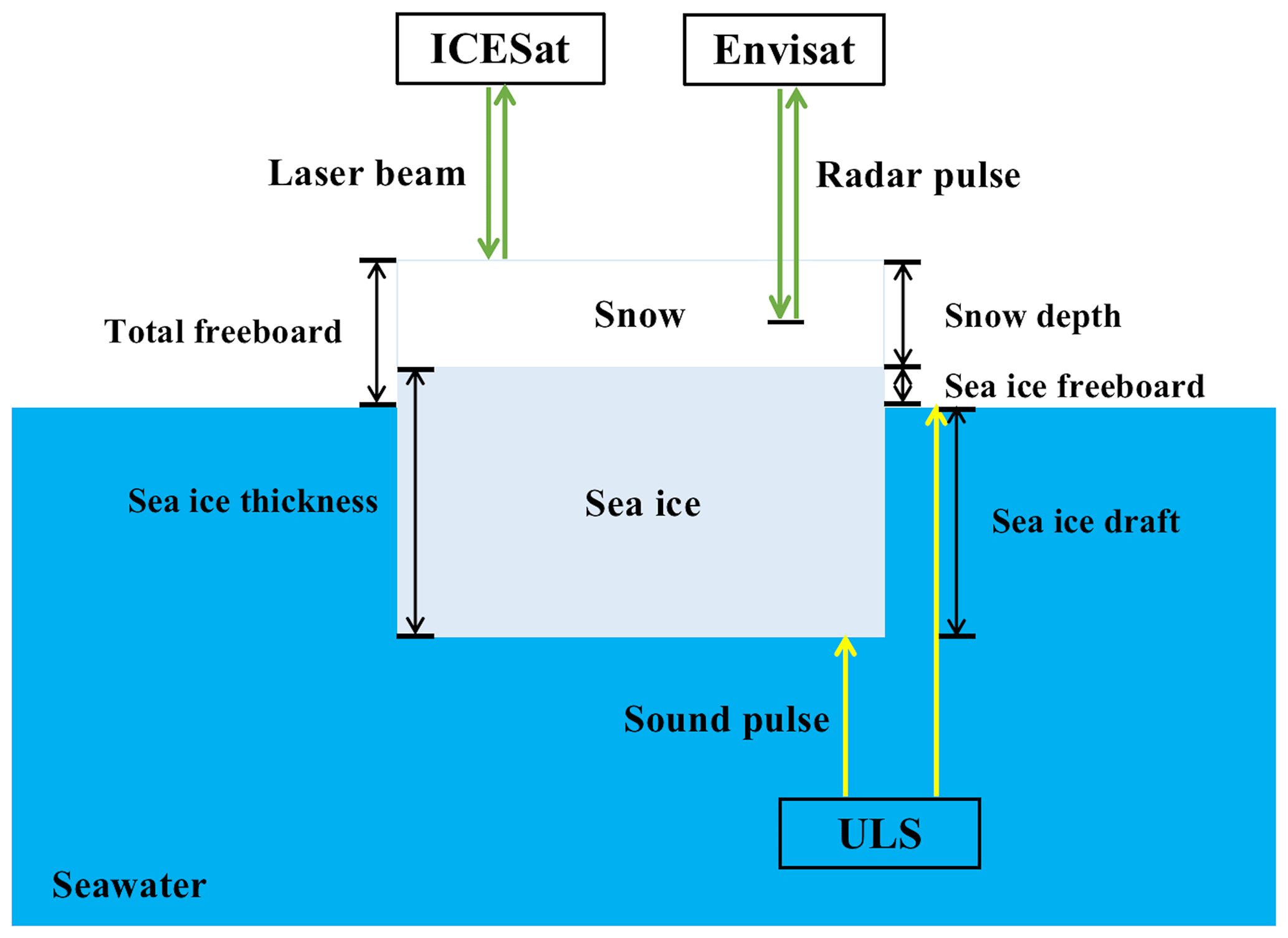
Figure 1An illustration of measuring freeboard using ICESat and Envisat and the ULS measurement principle. Note that radar altimeter on Envisat usually penetrates to somewhere between the air–snow and snow–ice interfaces (Willatt et al., 2010), which is one of the main sources of Envisat SIT uncertainties.
The Geoscience Laser Altimeter System (GLAS) aboard the Ice, Cloud, and land Elevation Satellite (ICESat) allows estimating the total freeboard through the determination of the surface elevation from 2003 to 2009, illustrated in Fig. 1. This data set has been used in previous studies for many years (e.g., Markus et al., 2011; Yi et al., 2011; Kurtz and Markus, 2012; Xie et al., 2013; Kern and Spreen, 2015). In contrast to radar altimetry, laser altimetry has the advantage of a well-defined reflective horizon, which is the air–snow interface. The main deficiencies of ICESat data are data gaps due to cloud coverage and more generally the discontinuous and short observation periods. Therefore, ICESat data cannot reflect the current characteristics of the fast-changing Antarctic sea ice. However, ICESat-2, which has been in orbit since 2018, provides a new source of year-round observations of total freeboard and better coverage than ICESat (Kwok et al., 2019; Kacimi and Kwok, 2020).
Both the Envisat and the CryoSat-2 SIT in the Southern Ocean have already been evaluated with the drilling, AEM, ULS and ship-based data (Kern et al., 2018). These evaluations are comprehensive but still have their limitations due to small spatial coverage or short temporal coverage. Thus, we cannot achieve an overall understanding of their data quality. To obtain a better understanding of the characteristics of the SICCI product version 2.0, we aim to investigate how the SICCI Envisat SIT compares with the ICESat SIT and also how the different altimeters and retrieval methods are represented in the SIT distribution. Based on the former inter-comparison study (Kern et al., 2016), we choose the ICESat SIT derived from the modified density approach for comparison, which seems to agree with average SIT from independent observations like ASPeCt, ULS and AEM and has a reasonable winter-to-spring growth (Kern et al., 2016). Furthermore, in order to evaluate the ICESat and Envisat data in the Weddell Sea, we also compare both SIT records with the Weddell Sea ULS data first.
The study is organized as follows. In Sect. 2, we describe the data used in this study in detail. Section 3 presents the results of both the Weddell Sea ULS data validations and the inter-comparisons between the two satellite data sets. Potential reasons for the spatial and temporal differences are discussed in Sect. 4. The main results are summarized in Sect. 5.
2.1 Sea ice thickness from Envisat RA-2
SICCI provides a set of Antarctic sea ice freeboard and thickness data (Hendricks et al., 2018b) obtained from the satellite missions Envisat (2002–2012) and CryoSat-2 (2010–2017). With 50 km grid resolution and monthly temporal resolution, there is a successive year-round record for Antarctic sea ice freeboard and thickness on the Equal-Area Scalable Earth (EASE) grid. Since only Envisat shares overlapping periods with ICESat, we focus on the characteristics of the Envisat radar altimeter. Envisat was launched on 1 March 2002, and the mission ended on 8 April 2012. The Radar Altimeter 2 (RA-2) aboard Envisat is a nadir-looking pulse-limited sensor operating at the main frequency of 13.575 GHz (Ku-band), with a secondary frequency of 3.2 GHz (S-band) compensating for the ionospheric error (Zelli and Aerospazio, 1999). It has an orbit inclination of 98.55∘, covering the whole ice-covered Southern Ocean, and nominal circular footprints of 2–10 km in diameter (Peacock and Laxon, 2004; Connor et al., 2009). Because RA-2 is the only altimeter carried by Envisat, we refer to it as Envisat hereafter.
The Envisat radar freeboard is retrieved based on the radar ranges obtained from RA-2 Level-1 waveform data over ice surface and leads between ice floes. Ideally, the signal will return at the interface between snow and ice based on experience from laboratory work (Beaven et al., 1995). Then, snow-depth-dependent radar signal delay is applied to convert the radar freeboard into the sea ice freeboard. An illustration of sea ice freeboard is shown in Fig. 1, which is the sea ice surface elevation relative to the sea surface elevation. Sea ice thickness is retrieved from sea ice freeboard based on the hydrostatic-equilibrium approach as first used by Laxon et al. (2003), who apply this method to ERS altimetry (ERS is the predecessor of the Envisat RA-2 instrument):
where F represents Envisat sea ice freeboard; S represents snow depth; I represents sea ice thickness; and ρwater, ρsnow and ρice refer to the densities of the seawater, snow and sea ice, respectively. A snow depth climatology is employed to retrieve sea ice thickness from sea ice freeboard here (Markus and Cavalieri, 1998; Comiso et al., 2003). This snow depth climatology is derived from the passive microwave sensors Advanced Microwave Scanning Radiometer for EOS (AMSR-E, 2002–2011, where EOS stands for Earth Observing System) and Advanced Microwave Scanning Radiometer 2 (AMSR2, 2012–2017), is based on a revised approach with different tie point retrieval plus addition of retrieval errors, and is provided by the Integrated Climate Data Center (ICDC).
In addition, it is noted that Envisat sea ice thickness represents the actual SIT (i.e., SIT of the ice-covered fraction of the grid cell area) and that values with sea ice concentration (SIC) of less than 70 % have been removed during Envisat SIT retrieval.
2.2 Sea ice thickness from ICESat GLAS
ICESat, operating as part of NASA's Earth Observing System, provides a set of Antarctic total freeboard from 2003 to 2009. Differently from the sea ice freeboard measured by radar altimeters, laser altimeters allow the detection of the distance between the snow surface and sea surface, as shown in Fig. 1. ICESat measurements are characterized by laser footprints of ∼ 70 m and sampling distances of 170 m (Kwok et al., 2004). However, the measurements are not continuous due to cloud coverage, and each measurement campaign lasted for about 35 d (see Fig. 3 in Kern and Spreen, 2015). There are several ICESat SIT data sets derived from different retrieval algorithms. Qualitative inter-comparisons have been made among several ICESat freeboard-to-thickness retrieval approaches (Kern et al., 2016). According to their conclusions, we choose the product derived with the modified density approach in this study because of its reasonable winter-to-spring increase and better agreements with independent data. The data set is provided by ICDC on the polar-stereographic grid. The approach considers the snow–ice layer as one system with a modified density in order to avoid using a potentially biased snow depth product. According to Kern et al. (2016), the modified density can be derived as follows:
where R is the ratio of sea ice thickness over snow depth, which is a seasonally dependent factor and calculated from ASPeCt observations (Worby et al., 2008a). And total thickness (sea ice thickness plus snow depth) can be determined from it as follows:
where F represents ICESat total freeboard. Although this method cannot obtain the real SIT, it still extracts the SIT information to a large extent. We will discuss the biases caused by this method in Sect. 4.
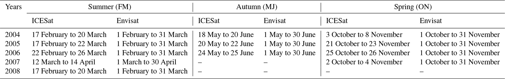
The Antarctic mean gridded total freeboard and effective sea ice thickness (i.e., mean thickness per grid cell including open-water areas) with a grid resolution of 100 km from 2004 to 2008 are provided in this product. Table 1 presents the available time periods of this data set. It is noted that grid cells with SIC of less than 60 % have been removed for the ICESat SIT retrieval.
Table 1ICESat operating periods and Envisat periods used for the comparisons. The three seasons are divided according to the ICESat operating periods. Note that ON is October–November, FM is February–March and MJ is May–June.
2.3 Sea ice thickness from Weddell Sea ULS
The upward-looking sonars (ULSs) located in the Weddell Sea provide long-term and high-frequency sea ice draft at each site (Behrendt et al., 2013a, b). The sensors transmit acoustic pulses upwards with a footprint of 6–8 m in diameter, and the signals are reflected by either the sea ice bottom or the sea surface, yielding a two-way travel time which can be converted into distances. The sea ice draft, which is the depth of the sea ice underwater, can consequently be derived from the difference in the two distances, shown in Fig. 1. The intervals of sea ice draft measurements are between 3 and 15 min from November 1990 to March 2008. In this study, we use the monthly average sea ice draft from 2004 to 2008 at three sites, corresponding to Envisat and ICESat operating time. According to Behrendt (2013), the uncertainties in sea ice draft vary from 0.05 to 0.12 m, depending on the seasons. The uncertainty in summer is smaller than in other seasons because open water occurs more frequently in the ULS footprint and thus the estimate of the sea surface height is more accurate. The mooring locations used in this study are shown in Fig. 2. Sea ice thickness (z) is converted from the sea ice draft (d) through an empirical formula established from drilling data in the Weddell Sea (Harms et al., 2001):
This empirical equation is based on the assumption that the snow depth values from drillings and ULS are comparable. But it still bears the uncertainties from the production of slush and snow ice caused by flooding (Harms et al., 2001). All the SIT data used in this study have been summarized in Table 2.
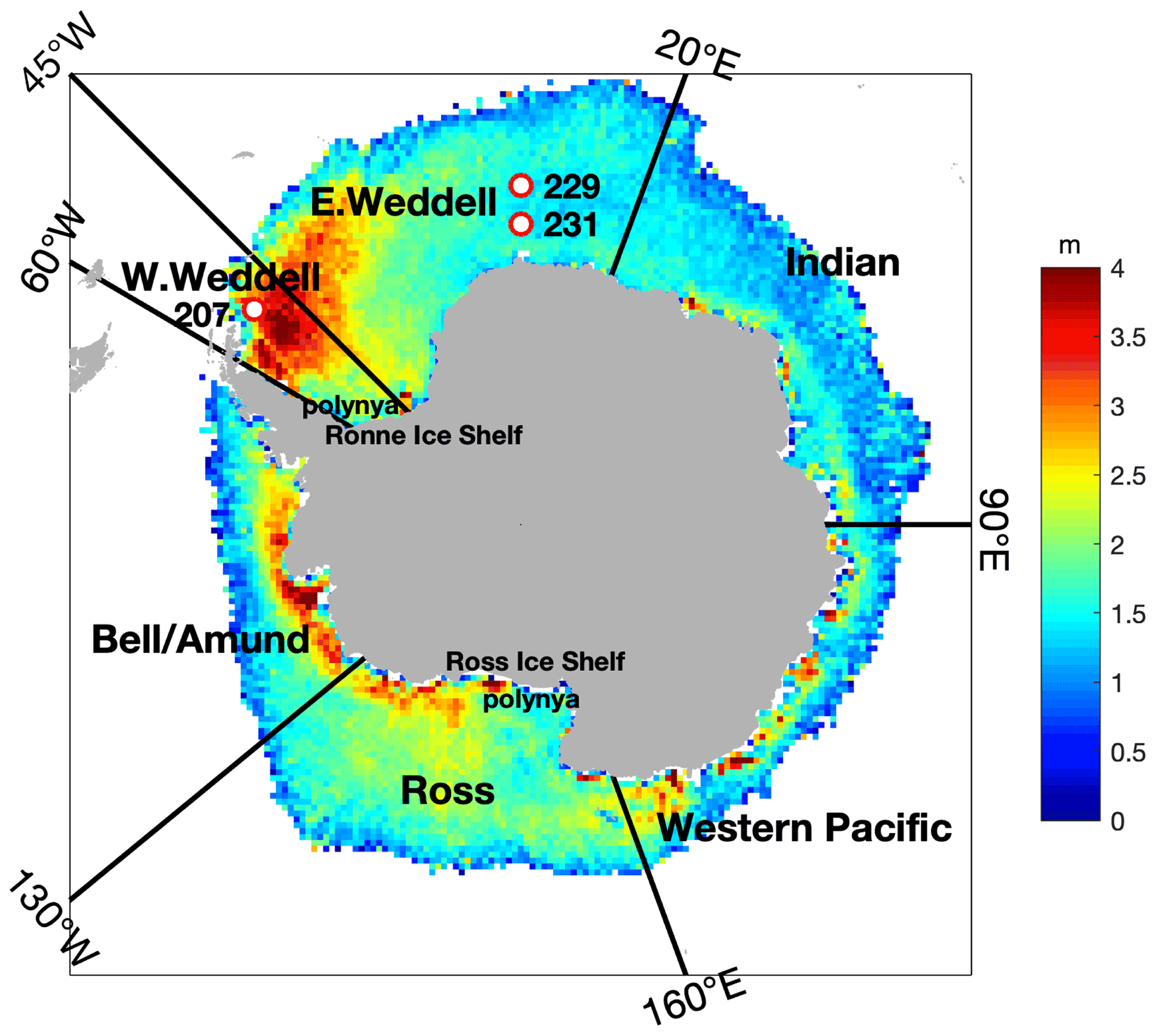
Figure 2Map of the different sectors referred to in the study. The background is the average of the September sea ice thickness from Envisat during 2003–2011 with 50 km grid size. Each sector and the two ice shelf polynyas are indicated in the figure. The circles and the corresponding numbers refer to the sites of the ULSs. The white grid cells stand for areas with sea ice concentration of less than 70 % or missing data.
Table 2A summary of the sea ice thickness data used during the comparison, including different data sources, spatial resolutions, temporal resolutions and snow products.

2.4 Spatial and seasonal divisions
The comparisons are made for different seasons and different sectors between the two SIT data sets. The seasonal classification is based on the ICESat operating periods presented in Table 1 following Kurtz and Markus (2012). For each ICESat operating period, we choose the corresponding Envisat monthly data, also given in Table 1. We employ a time-weighted average of the monthly Envisat data to match the ICESat period. For example, considering the ON04 period from 3 October to 8 November in 2004, which is 37 d long – 29 d in October and 8 d in November – we calculate the corresponding Envisat SIT as SIT. We use this weighing equation only for grid cells where valid Envisat SIT data exist in both months, while the weighing is not conducted for grid cells where valid data only exist in either one of the months. It is noted that this approach can lead to considerably larger coverage of Envisat SIT data than ICESat; thus we only show grid cells where both Envisat and ICESat have valid SIT and only take those values in the statistical computation.
Besides, since the Antarctic sea ice characteristics show regional differences, we divide the Southern Ocean into six sectors (Fig. 2) following Worby et al. (2008a) for the discussion.
3.1 Comparisons with Weddell Sea ULS
Before the inter-comparison between Envisat and ICESat SIT, both of them are compared with ULS observations. The ULS sea ice draft has been converted into monthly sea ice thickness data with Eq. (4) in Sect. 2.3. Both Envisat and ICESat SIT have been interpolated onto each ULS location in the nearest-neighbor way. In order to compare the SIT from the two satellites with the ULS observations, we first compute the ICESat effective SIT by dividing the SIT by the SIC at each grid cell. The SIC data are derived from the Special Sensor Microwave/Imager (SSM/I) and Special Sensor Microwave Imager/Sounder (SSMIS) based on the ASI algorithm provided by ICDC (Kaleschke et al., 2001; https://www.cen.uni-hamburg.de/en/icdc/data/cryosphere/seaiceconcentration-asi-ssmi.html, last access: 25 September 2020) with 12.5 km spatial resolution, interpolated to a 100 km National Snow and Ice Data Center (NSIDC) polar-stereographic grid and averaged over respective ICESat measurement periods. During ICESat operating periods, there are only three sites with valid data for the comparison: 207, 229 and 231 (shown in Fig. 2). The sites can be divided into two regions. Site 207 is near the coast of the Antarctic Peninsula, mostly characterized by perennial ice, while the others belong to the eastern Weddell Sea, predominantly characterized by first-year ice. The corresponding time periods of each SIT product are listed in Table 3.
Table 3Respective operation times of the ULS, Envisat (Env) and ICESat (ICE) sea ice thickness data sets during the comparison between ULS and satellite SIT.
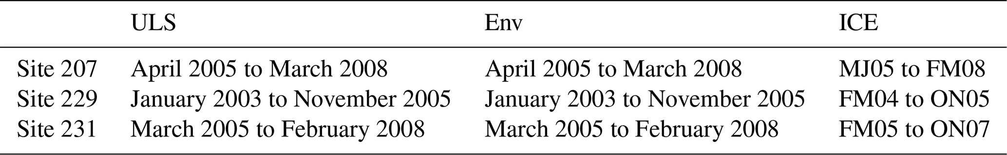
Figure 3 presents the time series of sea ice thickness for Weddell Sea ULS, Envisat and ICESat data at each site. Due to the operating-period gaps and lack of valid data along the coast, ICESat only provides a limited number of measurements for comparison. The gaps of Envisat SIT originate from grid cells with SIC below 70 % or missing data caused by failure of retrieval or of the instrument. The error bars show the uncertainty estimates for the respective SIT products. Envisat SIT uncertainties are computed as the error propagation of all input uncertainties with the assumption that the seawater density is negligible (see Sect. 2.9.8 in Paul et al., 2017). ICESat SIT uncertainties are also calculated based on the uncertainties in densities and freeboard (Kern et al., 2016). We also add the ULS error bars by calculating standard deviations (SDs) of the ULS SIT for each month. We find that either Envisat or ICESat SIT is not consistent with the sea ice thickness observed from ULSs. In the western Weddell Sea along the coast of the Antarctic Peninsula (at site 207), the ULS thickness ranges between 0 and 1.5 m, without a clear seasonal cycle due to a mixture of deformed and undeformed sea ice (Williams et al., 2015). Envisat thickness exceeds ULS thickness, with a maximum value larger than 5 m. In comparison, ICESat thickness also exceeds ULS thickness, and only a few ULS observations fall within the possible ICESat SIT range indicated by the error bars. In the eastern Weddell Sea (at sites 229 and 231), ICESat has a few overestimations while Envisat has larger overestimations. Note that the realistic ICESat SIT would be considerably smaller due to the retrieval method mentioned in Sect. 2.2, about 0.2–0.4 m at site 207 and 0.15–0.3 m at sites 229 and 231 depending on the seasons (Fig. S3). The differences in the error bars between Envisat and ICESat mainly result from their different spatial scales, the inclusion of snow depth uncertainty and lack of adequate regard for potential correlations between the error contribution in Envisat SIT, hence making it difficult to estimate realistic uncertainties. Table 4 shows the mean differences (MDs), SDs and root mean square deviations (RMSDs) for Envisat − ULS and ICESat − ULS and the numbers of comparison pairs. The Envisat and ULS SITs are all time-weighted, and the calculations are conducted when all three products have valid data. The statistics show that both MDs are the largest at site 207 (1.63 m for Envisat − ULS and 1.73 m for ICESat − ULS) and the smallest at site 229 (0.72 m for Envisat − ULS and 0.42 m for ICESat − ULS). However, the numbers of valid data are too small to derive a reliable conclusion on the accuracy of ICESat. The comparison is based on more data pairs for Envisat, but the agreement of the seasonal cycle is bad qualitatively (Fig. 3).
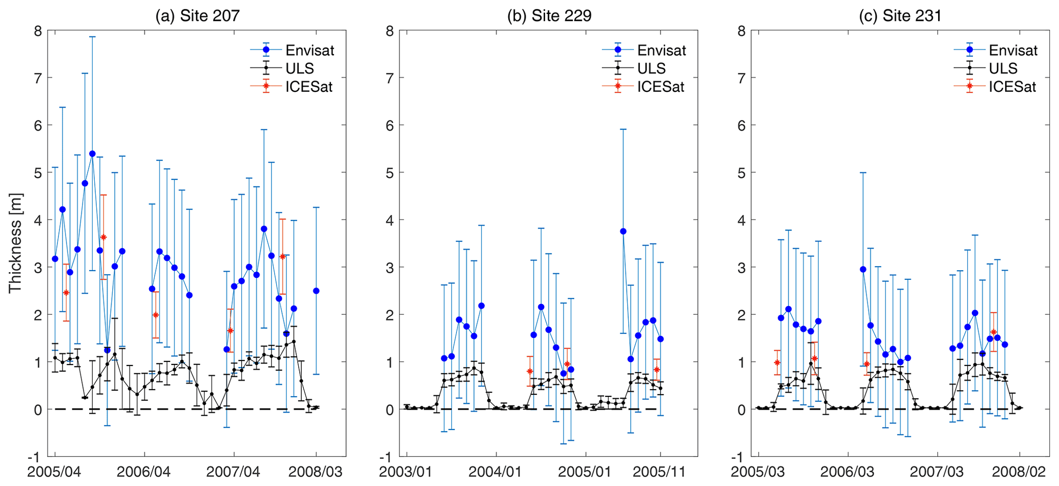
Figure 3Time series of sea ice thickness and their uncertainties for the Weddell Sea ULS data, Envisat and ICESat. The numbers at the top represent the location of each site for the comparisons. The site locations can be found in Fig. 2. ICESat SIT values are placed between the 2 months that each period covers. Time is given in the format year/month.
Table 4Statistical results of the comparison between two satellite SIT products with ULS data. N is the number of comparison pairs.

The uncertainties in such comparisons cannot be ignored. The ULS measurements are recorded at fixed locations with approximately 6–8 m footprint in diameter, while Envisat (ICESat) has a footprint of 2–10 km (70 m) and the SIT data used in the comparison represent mean values over 50 km (100 km) grid cells. Large resolution differences can increase the selection biases. While the ULS measures a single point like a ridge or the edge of thin ice, satellites will survey a large area. In addition, though the ULS SIT and satellite SIT are all monthly mean values, one ICESat SIT grid cell is scanned once or twice on most occasions through a measurement period (see Fig. 3 in Kern and Spreen, 2015). Averages based on such a small number of measurements have a limited representation of the mean SIT throughout the whole month. Theoretically, the more valid measurements exist in one grid cell, the more accurate the mean SIT. In general, uncertainties from both spatial interpolation and temporal representation can affect the comparisons. However, considering the typical sea ice motion (Drucker et al., 2011) in the Weddell Sea, monthly average ULS SIT could be referred to as a spatial average value, representing 100 km around the fixed ULS positions. With the sea ice motion data from NSIDC introduced in Sect. 2.4, the 30 d origins of the sea ice passing the three ULS sites from 2 July to 31 July 2011 are shown in Fig. S1, and they are spatially coherent.
3.2 Inter-comparisons between Envisat and ICESat
We first conduct an overall comparison between Envisat and ICESat effective SIT for each ICESat operating period in each season, as shown in Figs. 4–6. The effective Envisat SIT is calculated by multiplying the SIC contained in the data for each grid from OSI SAF Global Sea Ice Concentration (OSI-409) and the OSI SAF Global Sea Ice Concentration continuous reprocessing offline product (OSI-430) (http://osisaf.met.no, last access: 25 September 2020). The inter-comparisons are carried out by linearly interpolating Envisat SIT onto the ICESat polar-stereographic grid with 100 km grid resolution. The results suggest that there are substantial inter-seasonal and inter-annual differences between the two SIT data sets.
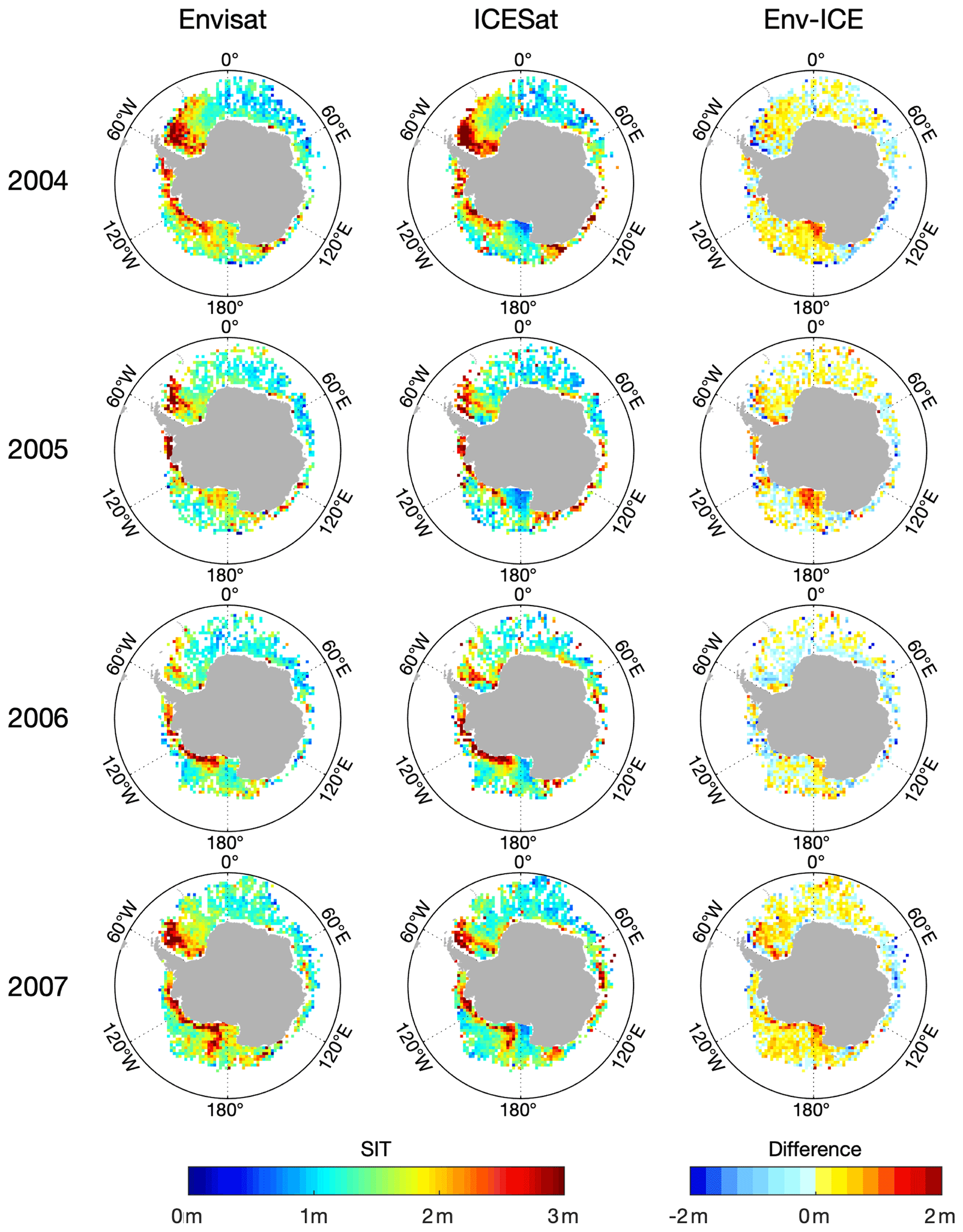
Figure 4Comparisons of Envisat versus ICESat sea ice thickness for each ICESat operating period in spring (October and November). The first and second columns show the sea ice thickness distribution of Envisat and ICESat, respectively, and the last column shows the difference field (Envisat minus ICESat) of sea ice thickness. Each row represents a year from 2004 to 2007. The maps are all interpolated onto the polar-stereographic grid of the ICESat product and only show grid cells where both data sets have valid SIT. The white cells denote sea ice concentration less than the threshold or missing data.

Figure 5Same as Fig. 4 but for summer (February and March).
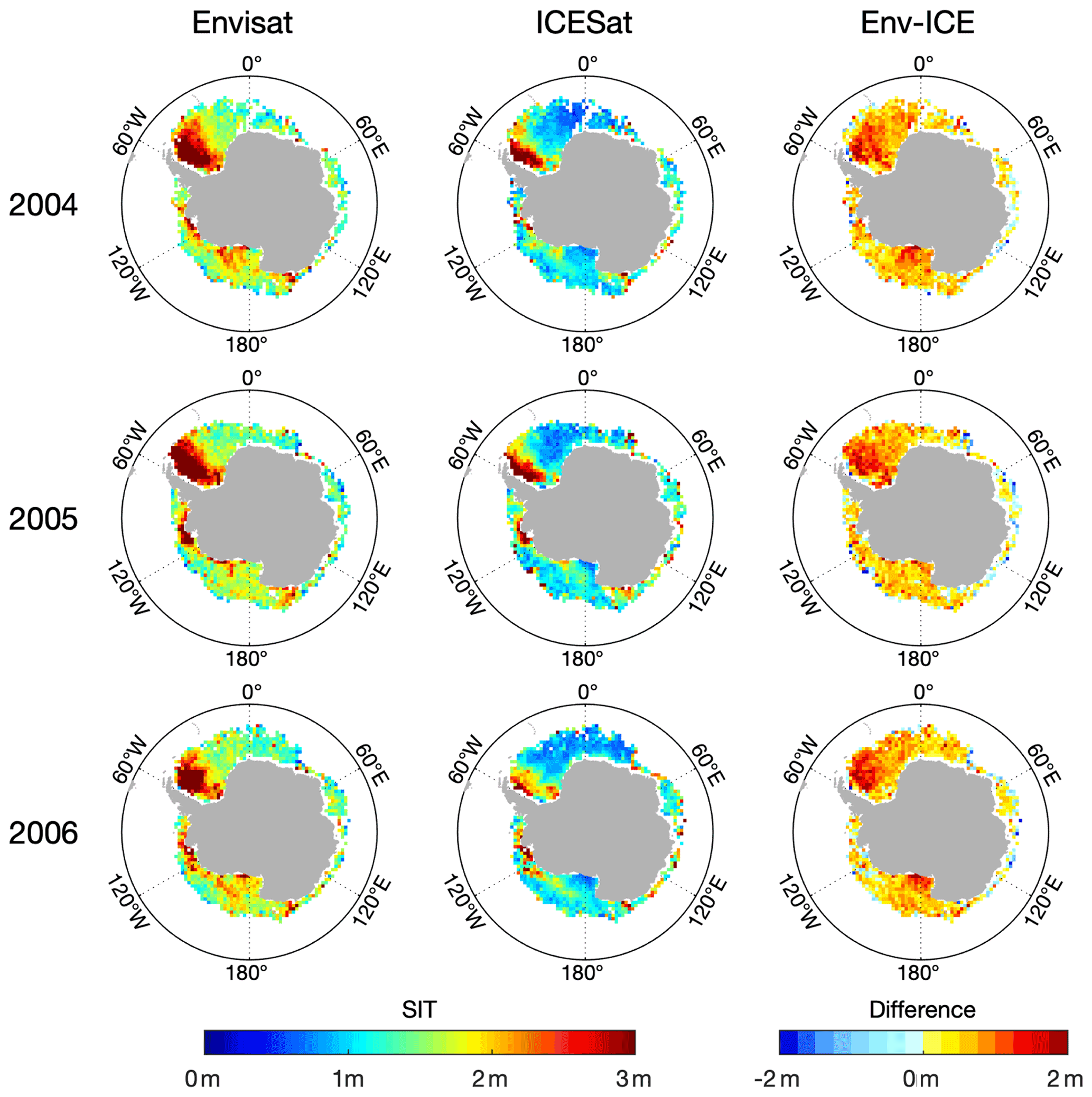
Figure 6Same as Fig. 4 but for autumn (May and June).
In spring (ON), both positive and negative differences exist between Envisat and ICESat SIT (Env − ICE), shown in Fig. 4. Envisat and ICESat are both able to capture the thick ice located in the western Weddell Sea and the Bellingshausen–Amundsen seas. Thick sea ice along the coast of the western Pacific Ocean is also detected by both sensors, but their mean SITs in 2004 are thicker than the ship-based observations (0.63 m; Worby et al., 2008a). The latter come from the average of 48 observations during the Aurora Australis cruise from 16 October to 7 November in 2004 covering 107–126∘ E. Note that a large SD (0.7 m) exists among the observations, and the ship-based estimates may not sufficiently represent the coastal sea ice. Thin ice in the Ross Sea is not captured by Envisat (Kern et al., 2018), while the Ross Ice Shelf polynya (indicated in Fig. 2) is present in the ICESat fields. Similarly, the Ronne Ice Shelf polynya appeared only in ICESat fields in 2007 but not in Envisat fields. A fringe with no data along most of the East Antarctic coast is caused by ICESat data gaps and indicates that the 100 km ICESat product fails to resolve the sea ice close to the coast. This can be attributed to a different land mask used in the ICESat product and consideration of lower freeboard quality there. Table 5 provides the respective SIT and their SDs, differences, RMSDs, correlation coefficients (CCs) and numbers of comparison pairs. In general, the difference between Envisat and ICESat spring SIT is close to zero, ranging from −0.16 m in 2006 to +0.10 m in 2007. However, these differences have to be seen in the light of the large SDs (∼ 0.6 m) and the fact that ICESat SIT values include the snow depth. The RMSD is the smallest by 0.39 m among three seasons, and CC is 0.68, with the significance larger than 95 %. Note that in order to obtain the seasonal mean SIT, we compute the seasonal mean SIT only from grid cells where values are available from both data sets and available for all 3 years in autumn, at least 3 of 4 years in spring and at least 3 of 5 years in summer. The numbers of grid cells used in the calculation are listed in the last column in Table 5.
Table 5Statistical results of the comparisons between Envisat sea ice thickness and ICESat sea ice thickness for each ICESat operating period. The correlation coefficients (CCs) in italic type have not passed the 95 % significance test. N is the number of comparison pairs.
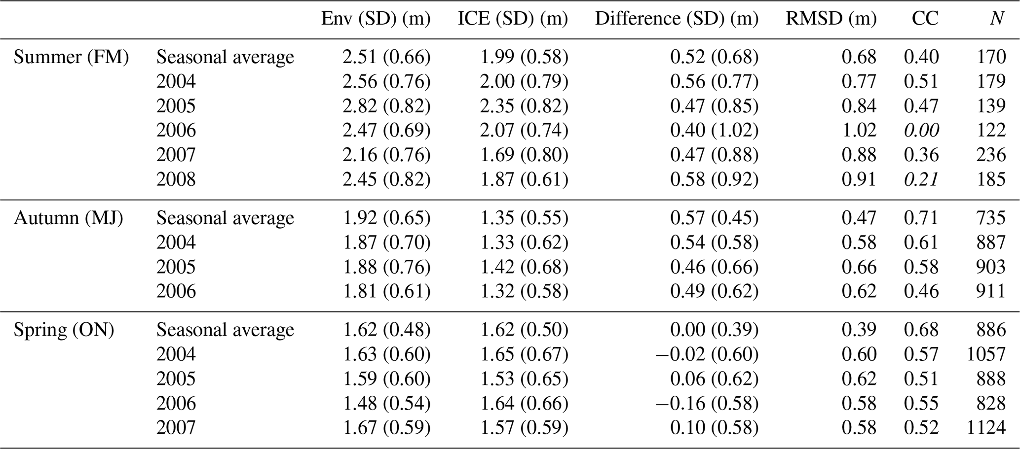
At the end of summer melt (FM), the ice coverage is limited to the western Weddell Sea, Bellingshausen–Amundsen seas along the coast and southern Ross Sea (Fig. 5). In the western Weddell Sea, Envisat shows that thick ice still exists and remains at least 3 m thick, while ICESat shows thinner ice. As for the Ross Ice Shelf polynya, ICESat displays thin ice lower than 1 m in 2004, 2007 and 2008, while Envisat detects sea ice of up to 1.5 m, much larger than expected seasonal ice thickness. According to Table 5, the numbers of comparison pairs are small. Generally, Envisat SIT exceeds ICESat SIT by 0.52 m in summer, with the largest RMSD by 0.68 m and the smallest correlation values by 0.40 among the three seasons. Considering the ICESat SIT excluding snow depth, the real differences should be larger.
In autumn (MJ), SIT patterns of the two data sets are comparable, shown in Fig. 6. The differences between Envisat and ICESat SIT are consistently positive over all regions except some regions in the East Antarctic. Compared with summer, the positive differences in the western Weddell Sea expand to positive differences over the whole Weddell Sea sector, and the differences decrease from west to east. In addition, positive differences in the Ross Ice Shelf polynya still exist, mostly due to Envisat's inability to capture the thin ice there (Comiso et al., 2011; Tian et al., 2020), which has been pointed out in Kern et al. (2018), who identified a substantial SIT difference between Envisat and CryoSat-2 in that region. According to Table 5, despite the largest mean difference (0.57 m) and large RMSD (0.47 m), the correlation in autumn is actually the highest of the three seasons investigated (0.71).
To investigate the development of two SIT data sets from the end of melting to the end of freezing, we provide the probability distribution of the Envisat SIT and the ICESat SIT for all the valid individual comparison pairs where both Envisat and ICESat have valid SIT, shown in Fig. 7. The mean and modal SITs of both data sets are marked besides. In summer, the agreement between Envisat SIT and ICESat SIT is not good, mainly due to their different performance on thick ice in the Weddell Sea (Fig. 5). Envisat still presents a larger mean and modal thickness than ICESat in autumn. In spring, the two data sets have similar distributions, represented by similar mean and modal thicknesses. In addition, we find that ICESat mean SIT increases while Envisat mean and modal SIT decreases from autumn to spring. For Envisat SIT, the distribution indicates that more ice is in thinner categories in spring than autumn, while more ice in thicker categories is found for ICESat SIT. Therefore, we further compare the mean variations in Envisat SIT, ICESat SIT, Envisat freeboard, ICESat freeboard and snow depth climatology used in Envisat retrieval from autumn (MJ) to spring (ON), shown in Fig. 8. The average fields are calculated with grid cells where both Envisat and ICESat SIT have valid values in all 3 years from 2004 to 2006. Figure 8 shows that Envisat SIT experiences general decreases from May–June to October–November (MJON) except in the Bellingshausen Sea and part of the Amundsen Sea. Significantly large decreases exist in the western Weddell Sea. In contrast, ICESat SIT presents large-scale increases except in the western Weddell Sea and Ross Sea where slight decreases exist. By comparing the SIT and freeboard changes of both products, we find that the freeboard differences dominantly explain the SIT differences. Based on our analyses above and the common assumptions during ice freeze-up, the Envisat freeboard is likely overestimated in autumn, as has been previously pointed out in several studies (e.g., Willatt et al., 2010; Kwok and Kacimi, 2018; Kacimi and Kwok, 2020). Moreover, the decreased snow depth climatology in the western Weddell Sea and Ross Sea (Fig. 8e) also contributes to the Envisat SIT change, which has been reported by Kern and Ozsoy-Çiçek (2016), who found that AMSR-E snow depth is likely to underestimate the snow depth evolution during MJON.
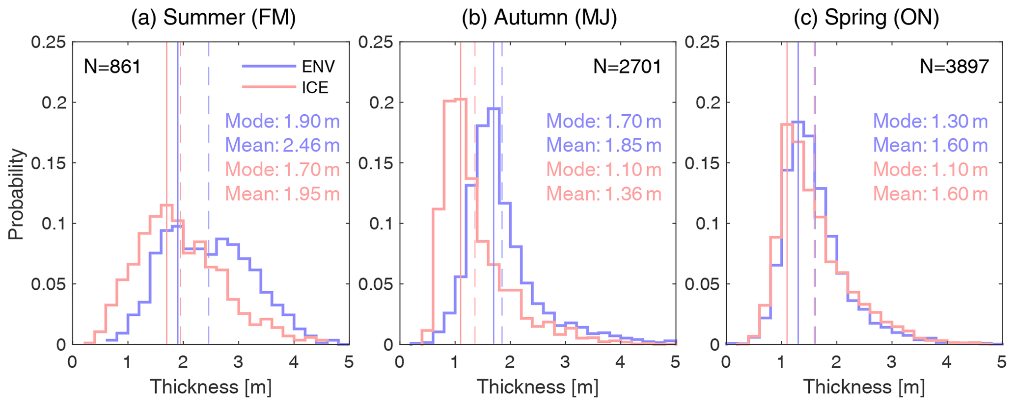
Figure 7Probability of the Envisat SIT and the ICESat SIT for all the individual comparison pairs. The blue stairs represent Envisat ice thickness, and the red stairs represent ICESat ice thickness. The solid lines indicate the modal ice thickness, and the dashed lines indicate the mean ice thickness of both data sets. The bin size is 0.2 m, and the probability distribution is normalized.
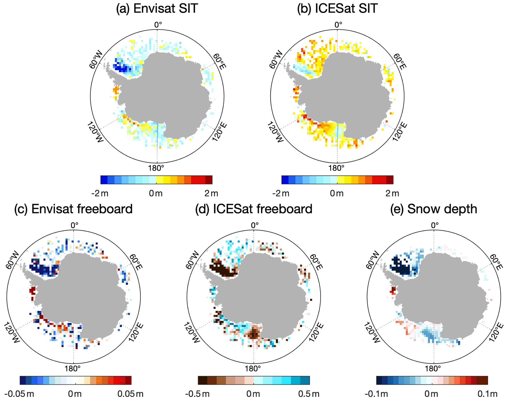
Figure 8The average changes in Envisat SIT, ICESat SIT, Envisat freeboard, ICESat freeboard and snow depth climatology used in Envisat retrieval from autumn to spring (MJON) calculated from 2004, 2005 and 2006.
Figure 9 presents scatterplots of the individual comparison pairs between Envisat SIT and ICESat SIT for each region and each season. Respective CCs and RMSDs are indicated in the panels. Due to the limited measurements in the Indian Ocean and western Pacific Ocean, we combine them into the whole East Antarctic. For all five sectors, Envisat SIT tends to exceed ICESat SIT on thin ice. From Fig. 9a, we can see that in the western Weddell Sea, the summer and autumn SIT clouds exceed the spring ones. This reveals that ICESat SITs are nearly constant through all three seasons in the western Weddell Sea, while Envisat SITs are noticeably larger in summer and autumn, also shown in Table 6. From FM to ON, Envisat SIT changes from 3.01 to 3.18 to 2.23 m, while ICESat SIT changes from 2.04 to 2.28 to 2.23 m. Considering the regional average differences between Envisat and ICESat SIT, the largest difference (0.63 m) is found in the western Weddell Sea and the smallest is in the Bellingshausen–Amundsen seas (0.09 m). Differences are small during spring for all regions except the East Antarctic. The largest CC is found during autumn for the Bellingshausen–Amundsen seas (0.58), and the smallest is during autumn for the Ross Sea (0.1).
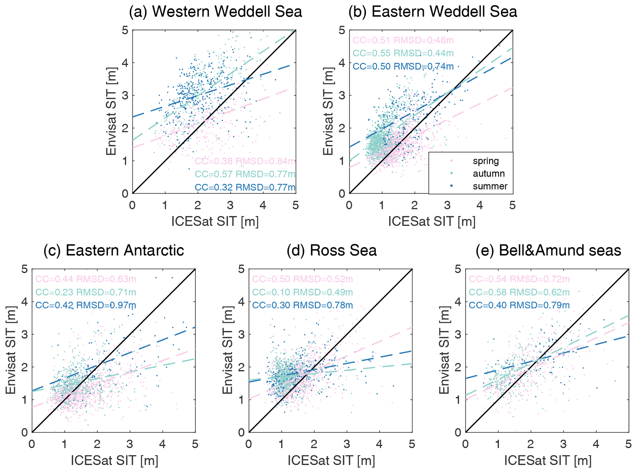
Figure 9Scatterplots of the individual data pairs between Envisat SIT and ICESat SIT for each region and each season. The data are taken from all seasons available. Since the comparison pairs are too few in the Indian Ocean and western Pacific Ocean, we combine these two regions into the East Antarctic. The respective correlation coefficients and RMSDs are indicated in the panels. The black line is the 1-to-1 fit line, and the dashed colored lines stand for linear regression lines.
Table 6Statistical results of the comparisons between Envisat sea ice thickness and ICESat sea ice thickness for each region divided as in Fig. 9. N is the numbers of comparison pairs, taking into account the actual number of values per season. Bell/Amund denotes the Bellingshausen and Amundsen seas.

There are two main differences between the two data sets. For one they use different sensors to determine surface elevation and freeboard. Envisat is equipped with a Ku-band radar altimeter (RA-2) whose backscatter is assumed to originate from the snow–ice interface. It is known that this assumption is flawed for snow that is wet, not cold and without a homogenous stratigraphy (Willatt et al., 2010). Instead, ICESat is equipped with a laser altimeter (GLAS) whose signals are reflected from the air–snow interface. In addition, considering the large pulse-limited Envisat footprint of about 2–10 km and smaller footprint of ICESat laser beams of about 70 m, there are very likely differences in the ability to resolve leads or open water required for an adequate representation of the local sea surface height during the freeboard retrieval, as well as in the accurate representation of heterogeneous sea ice surfaces. The other difference is that they apply different retrieval algorithms to convert freeboard into thickness. Envisat directly uses the hydrostatic equilibrium together with a snow depth climatology derived from AMSR-E and AMSR2 data, while ICESat uses the hydrostatic equilibrium accompanied with a modified snow–ice density method to reduce the influence of the often regionally biased snow depth product. The effects of these differences between both products are discussed in the following.
4.1 Differences due to sensors
It is assumed that the dominant backscatter horizon for a Ku-band radar altimeter is the snow–ice interface for cold and dry snow (Beaven et al., 1995). However, this would not always be the case in the Southern Ocean according to the field investigations conducted by Willatt et al. (2010). They demonstrate that the dominant scattering surface of the Ku-band radar lies within the snowpack, usually at half of the mean snow depth, when the snow cover is not cold and dry. Wet conditions can affect the dielectric properties of snow and then weaken the penetration of radar altimeter signals into the snow. Consequently, RA-2 range measurements could be biased high when the main scattering horizon is located within the snowpack, which would lead to larger sea ice freeboard and larger sea ice thickness. The salinity of the basal snow layer also contributes to this effect (Nandan et al., 2017). Such biases are also shown by Kwok and Kacimi (2018), where they find that radar freeboard values from CryoSat-2 are consistently higher than those computed using Operation IceBridge (OIB) measurements. Other studies that utilize CryoSat-2 radar data in the Southern Hemisphere have thus explicitly incorporated radar backscatter from the snow layer into their freeboard retrieval method (Fons and Kurtz, 2019).
The sensitivity of Envisat SIT (I) to sea ice freeboard (F) can be calculated from Eq. (1):
We set ρwater to 1024 kg m−3 and use ρice values between 880 and 940 kg m−3 to cover all mixed types of sea ice. Figure 10a illustrates the sensitivity of the sea ice thickness changes in response to sea ice density and sea ice freeboard biases between 0.02 and 0.1 m in steps of 0.02 m. We can see that SIT changes range from 0.14 to 1.22 m with different freeboard biases and density in our experiment. With the increase in freeboard biases and sea ice density, SIT changes become larger. Under larger-freeboard-bias conditions, SIT changes climb faster as density rises. For typical sea ice freeboard biases caused by saline snow (0.07 m for the Arctic nominal adjustment for first-year ice suggested by Nandan et al., 2017, 2020), the sea ice density variations induce the thickness changes ranging from ∼ 0.5 to ∼ 0.8 m. This could potentially account for the differences between Envisat and ICESat SIT in autumn (0.57 m). Therefore, we assume that in autumn freeboard-bias-induced SIT changes happen frequently. In summer, when snow salinities are significantly lower than measurements in other seasons (mostly below 0.1‰) but the wetness is high at the snow bottom (Haas et al., 2001), the freeboard biases also matter because liquid water content affects the snow dielectric properties (Barber et al., 1995). Besides, based on previous studies (Willatt et al., 2010; Kwok and Kacimi, 2018; Kacimi and Kwok, 2020), the displacements of radar retracking points and thus the freeboard biases can be significant in spring. Considering the small differences between Envisat and ICESat SIT, we suggest that underestimations of snow depth and biases in ICESat total thickness might play an important role in spring. However, detailed sensitivity discussions are limited due to lack of seasonal and regional sea ice density and adjustments to sea ice freeboard.
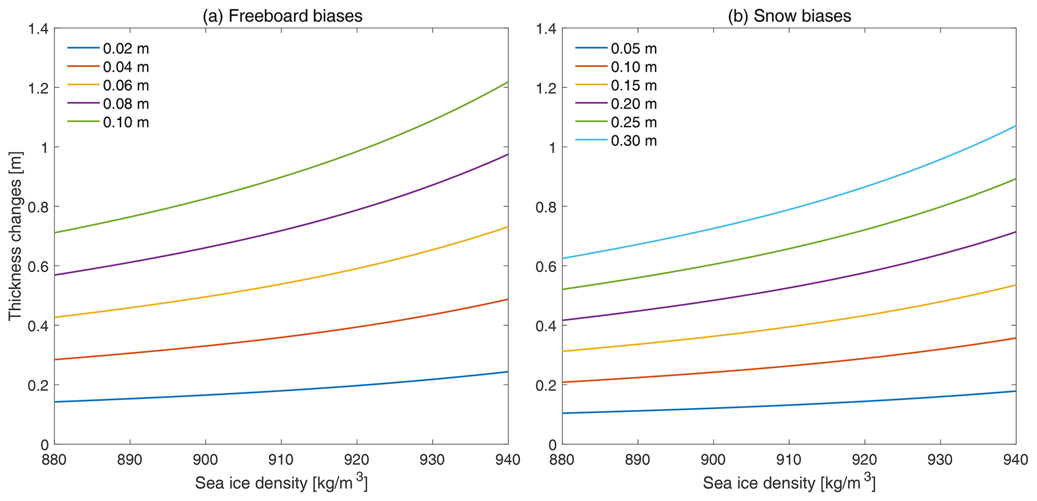
Figure 10Sensitivity of sea ice thickness changes to sea ice freeboard biases and snow depth biases as a function of sea ice density. (a) SIT changes computed with Eq. (1) for different sea ice freeboard biases (0.02 to 0.1 m). (b) Similar to (a) but computed for different snow depth biases (0.05 to 0.3 m).
In addition to the different penetration depths, the two sensors have different footprints. Envisat is a pulse-limited radar altimeter with a large footprint of 2–10 km, and ICESat is a laser altimeter with a small footprint of about 70 m. This makes them sensitive to a relative selection bias, primarily on the side of the altimeters with the lower resolution in the case of surface-type mixing within the footprint, especially if the different surface types vary in their backscatter properties. Higher spatial resolution will mitigate this issue and subsequently allow a better classification of lead and sea surface height retrieval in principle. Several studies have pointed out that Envisat freeboard and thickness uncertainties are elevated with respect to other sensors due to sub-footprint-scale surface-type mixing (Schwegmann et al., 2016; Paul et al., 2018; Tilling et al., 2019). While this is also directly applicable to radar altimeters with different footprints, the response to lead surfaces of laser (ICESat) and radar (Envisat) altimeters is directly a function not only of footprint size but also of the altimeter concept. Leads dominate radar backscatter even if the leads are already covered by thin sea ice for nadir and off-nadir cases and thus cause an overrepresentation of lead detections with range biases for off-nadir leads in Envisat data. Off-nadir reflections are usually detected and removed from the freeboard retrieval, resulting in an underrepresentation of areas with mixed surface types in the Envisat freeboard statistics. Lead laser backscatter instead is a function of the surface albedo; thus leads return lower laser backscatter power, and since ICESat footprints do not overlap, the lead oversampling and necessary filtering of off-nadir reflections are not an issue for laser altimetry. For variable ice surfaces, the smaller footprint of ICESat has the capability to provide more detailed observations in areas with heterogeneous ice conditions than the pulse-limited Envisat footprint.
4.2 Differences due to snow depth
Another source of the differences is the AMSR-E snow depth. AMSR-E snow depth is retrieved from brightness temperature based on the linear relation between brightness temperatures and in situ observations (Markus and Cavalieri, 1998; Comiso et al., 2003). According to Markus and Cavalieri (1998), their AMSR-E snow depth product is limited to the maximal retrieval value being around 0.50 m because of the saturation of the signal; i.e., there is no change in the brightness temperature gradient ratio with increasing snow depth over a certain limit. Previous studies have shown that AMSR-E snow depth tends to considerably underestimate the actual value over deformed sea ice, which usually occurs in the East Antarctic (Worby et al., 2008b; Ozsoy-Çiçek et al., 2011). According to Kern and Ozsoy-Çiçek (2016), AMSR-E snow depths minus the ASPeCt observations are positive for snow below 0.15 m and negative for snow above 0.3 m. Environmental conditions have great effects on the snow physical properties such as density, wetness and salinity, and passive microwave snow depth is sensitive to ice concentration errors, weather effects, grain size, thaw and refreezing (Markus and Cavalieri, 1998). Particularly, wet snow caused by melting or flooding could lead to underestimations of snow depth while refreezing of wet snow could lead to overestimations. All of the above biases can affect the differences between Envisat and ICESat SIT.
According to Eq. (1), we can derive the sensitivity of Envisat SIT (I) to snow depth (S):
Setting ρsnow=300 kg m−3 and taking the same values for water and sea ice density as in Eq. (5), we can see how SIT changes in response to sea ice density and snow depth biases between 0.05 and 0.3 m in steps of 0.05 m, shown in Fig. 10b. Thickness changes rise as snow biases become larger and also with larger sea ice density. However, compared with Fig. 10a, SIT changes are more sensitive to freeboard biases than to snow biases. For 880 kg m−3 density, SIT only changes by 0.1 m every 0.05 m snow bias but by 0.14 m every 0.02 m freeboard bias. With typical snow depth biases (0.2 m for the monthly mean retrieval uncertainty in Kern and Ozsoy-Çiçek, 2016), the thickness changes from ∼ 0.4 to ∼ 0.7 m. Therefore, snow depth bias is also a critical factor contributing to the difference between Envisat and ICESat SIT. In general, passive microwave snow depth is valid over level ice. During FM, snow is deep, potentially wet and/or metamorphous on thick ice, causing substantial difficulties for radar altimeters. And for the same reasons, passive microwave snow depth is possibly underestimated on thick ice not only during FM but also during other seasons. These snow depths also underestimate actual snow depth over deformed ice mostly during ON in the East Antarctic and Bellingshausen and Amundsen seas (Kwok and Maksym, 2014; Kacimi and Kwok, 2020).
Additionally, more significant effects might come from the differences between actual snow depth and that represented by the climatology. During the Envisat SIT retrieval, the snow depth climatology is employed neglecting the inter-annual snow variability. According to Bunzel et al. (2018), the impact of using a snow depth climatology is small when the snow depth is thin. The application of snow depth climatology in the SIT retrieval allows reducing the relative uncertainties compared with the actual snow depth values, which are affected by several factors as discussed above and have large uncertainties. However, it may also lead to an adverse outcome when the climatology is constructed from biased snow depth data, as is the case for the Envisat SIT retrieval. To further quantify the differences between snow depth climatology and actual snow depth contributions, we simulate the retrieval of Envisat SIT by replacing the snow depth climatology with monthly SICCI AMSR-E snow depth provided by SICCI (Kern et al., 2015). The new Envisat SIT is converted through Eq. (1) with Envisat monthly gridded sea ice freeboard data, monthly AMSR-E snow depth and the same density values mentioned above. The new Envisat SIT is compared with ICESat SIT, and the changes to former Envisat − ICESat differences are shown in Table S1. This result reveals that the impacts of snow depth climatology are larger in the Bellingshausen–Amundsen seas and the western Weddell Sea compared to other sectors. Among the three seasons, the changes are larger in summer, partly accounting for the differences between Envisat and ICESat SIT.
Moreover, the distance between sea ice surface elevations and the sea surface height is computed with vacuum light speed, which is defined as radar freeboard (RFB). A geometric correction used to correct the slower wave propagation speed in the snow layer is applied to convert the radar freeboard into the sea ice freeboard (FB):
But the delay correction is based on a conventional assumption that has been assessed by Mallett et al. (2020), which pointed out that it introduced systematic underestimation of up to 0.15 m into SIT estimates. While this systematic bias is small compared to those of other sources, uncertainties in snow depths and incomplete radar wave penetration would cause larger biases in this way.
4.3 Differences due to ICESat biases
The modified density method used by Kern et al. (2016) does not consider the small-scale or regional variability in the snow depth. Instead, only a seasonal constant density derived from the ASPeCt observations is given. Therefore, the largest uncertainty in ICESat comes from the potential underestimations of the ship-based sea ice thickness and snow depth observations for the computation of the bulk density of the ice–snow column (Kern et al., 2016). This bias has been modified in Li et al. (2018), who derived first-guess values of snow depth and sea ice thickness directly from ICESat data with empirical approaches, instead of the observation climatology used by Kern et al. (2016). Besides, this method is actually providing the total (sea ice plus snow depth) thickness. Taking this into account, the actual ICESat SIT shown in this paper would possibly even be a bit smaller. To examine this issue, we subtract the snow depth climatology (used in Envisat retrieval) from the ICESat data and compare this with Envisat thickness. The changes to the former differences are shown in Table S2, which is also a representation of the snow depth climatology itself. Larger variations exist in the western Weddell Sea, especially in summer and autumn. In general, variations are smaller than 0.5 m, yet they lead to larger positive differences between Envisat and ICESat SIT. More realistic SIT data are derived in Xu et al. (2021) by subtracting the snow depth. However, we do not aim to choose the best ICESat SIT product with the most real SIT but to investigate the causes of the differences between Envisat and ICESat SIT and how different sensors and retrieval methods are represented in the SIT fields.
Apart from the uncertainties from the ICESat retrieval method mentioned above, Kern et al. (2016) also discussed the potential biases due to total freeboard and sea ice density. In comparison with the freeboard from Kurtz and Markus (2012), modal and mean total freeboard values of this product are slightly higher, which might be a potential source of SIT positive biases. The total freeboard retrieved from ICESat has an uncertainty of up to 0.1 m, mainly due to the choice of the percentage of observations used as sea surface height tie points (Kern and Spreen, 2015). Meanwhile, a smaller sea ice density will lead to smaller modified ice–snow density and SIT according to Eqs. (2) and (3). We analyze the sensitivity of ICESat SIT to sea ice density and find an increase of ∼ 0.2–0.4 m SIT when sea ice density rises from 880 to 940 kg m−3 under seasonal R values and total freeboard.
In this study, we compare SIT estimates of the sea ice thickness obtained from satellite altimeter observations by Envisat RA-2 (radar) and ICESat GLAS (laser) in the Southern Ocean. Envisat and ICESat SIT are compared with ULS SIT in the Weddell Sea, with the MDs (SDs) of 1.29 (0.65) m for Envisat − ULS and 1.11 (0.81) m for ICESat − ULS. Then a systematic comparison between the two data sets is carried out for all seasons except winter, based on the ICESat operating periods. According to the results, the differences between Envisat and ICESat SIT vary from season to season, year to year and region to region. Specifically, the smallest monthly average difference (SD in parentheses) for Envisat SIT minus ICESat SIT exists in spring with 0.00 m (0.39 m), while larger differences (SD) exist in summer and autumn with 0.52 (0.68 m) and 0.57 m (0.45 m), respectively. In spring, ICESat SIT fields reveal the Ross Ice Shelf polynya, while it is not present in the Envisat data. In summer, the derived Envisat data show that thick ice still exists in the western Weddell Sea and remains at least 3 m thick every year, while ICESat shows thinner ice. Compared to summer, the positive differences in the western Weddell Sea expand to the whole Weddell Sea sector and slightly decrease from west to east in autumn. From the probability distribution, it is noted that Envisat and ICESat have different SIT variations from autumn to spring – i.e., ICESat SIT increases while Envisat SIT does not – but share similar SIT growth from summer to autumn. Compared to the average changes in Envisat freeboard, ICESat freeboard and snow depth climatology used in Envisat retrieval during MJON calculated from 2004, 2005 and 2006, we assume the main reason for the Envisat SIT decrease is the overestimation of Envisat freeboard in autumn and the underestimation of snow depth evolution during MJON. With respect to different sectors, the regional MDs (SDs) are 0.63 m (0.91 m) in the western Weddell Sea, 0.34 m (0.58 m) in the eastern Weddell Sea, 0.31 m (0.57 m) in the Ross Sea, −0.12 m (0.69 m) in the East Antarctic and 0.09 m (0.71 m) in the Bellingshausen–Amundsen seas. Our sensitivity experiments show that Envisat SIT changes are more sensitive to sea ice freeboard biases than to snow depth biases. Additionally, increasing sea ice density causes larger SIT changes. Usage of snow depth climatology has moderate impacts on SIT estimates in the summer Bellingshausen–Amundsen seas and western Weddell Sea. Moreover, ICESat SIT can have an increase of ∼ 0.2–0.4 m when sea ice density rises from 880 to 940 kg m−3 under seasonal R values and total freeboard.
While we choose one of the ICESat SIT products to conduct the comparison, there are several other ICESat SIT products using different retrieval algorithms available, e.g., the SICCI product discriminating between positive and negative sea ice freeboard (Kern et al., 2016) or the one assuming zero sea ice freeboard in freeboard-to-thickness conversion (Kurtz and Markus, 2012). These different products provide a range of values within which ICESat SIT may be located; thus the differences between Envisat and ICESat SIT in this study are just one of the possible outcomes.
Through the study, we acknowledge that there are differences between Envisat and ICESat sea ice thickness, which potentially result from the biases within each of the two data sets. There is still more work to be done to make better use of remotely sensed SIT data, such as assimilating the Antarctic sea ice thickness observations and analyzing the sea ice volume variations.
Envisat sea ice thickness data are available at https://doi.org/10.5285/b1f1ac03077b4aa784c5a413a2210bf5 (Hendricks et al., 2018b). ICESat sea ice thickness data are available at https://www.cen.uni-hamburg.de/en/icdc/data/restricted-access/esa-cci-antarctic-sea-ice-thickness.html (Kern et al., 2016). The Weddell Sea upward-looking sonar data are available at https://doi.org/10.1594/PANGAEA.785565 (Behrendt et al., 2013a, b). NSIDC sea ice motion data are accessible at https://doi.org/10.5067/INAWUWO7QH7B (Tschudi et al., 2019). AMSR-E snow depth data are accessible at https://www.cen.uni-hamburg.de/en/icdc/data/restricted-access/esa-cci-antarctic-snow-depth.html (Markus and Cavalieri, 1998).
The supplement related to this article is available online at: https://doi.org/10.5194/tc-16-4473-2022-supplement.
QS developed the concept of the paper. JW analyzed the data and wrote the manuscript. CM, RR, QS, BH, SH, RW and QY assisted during the writing process.
The contact author has declared that none of the authors has any competing interests.
Publisher’s note: Copernicus Publications remains neutral with regard to jurisdictional claims in published maps and institutional affiliations.
This article is part of the special issue “The Weddell Sea and the ocean off Dronning Maud Land: unique oceanographic conditions shape circumpolar and global processes – a multi-disciplinary study (OS/BG/TC inter-journal SI)”. It is not associated with a conference.
The authors wish to thank the editor and anonymous reviewers for their very helpful comments and suggestions. This is a contribution to the Year of Polar Prediction (YOPP), a flagship activity of the Polar Prediction Project (PPP), initiated by the World Weather Research Programme (WWRP) of the World Meteorological Organization (WMO). We acknowledge the WMO WWRP for its role in coordinating this international research activity. The authors would like to thank the Alfred Wegener Institute, Helmholtz Centre for Polar and Marine Research for providing the Weddell Sea upward-looking sonar data and the Integrated Climate Data Center at the University of Hamburg for providing the ICESat sea ice thickness data.
This study is supported by the National Natural Science Foundation of China (grant nos. 41941009, 41922044), the National Key R&D Program of China (grant no. 2022YFE0106300), the Guangdong Basic and Applied Basic Research Foundation (grant no. 2020B1515020025), and the fundamental research funds for the Norges Forskningsråd (grant no. 328886).
This paper was edited by Petra Heil and reviewed by four anonymous referees.
Barber, D. G., Reddan, S. P., and LeDrew, E. F.: Statistical characterization of the geophysical and electrical properties of snow on Landfast first-year sea ice, J. Geophys. Res., 100, 2673–2686, https://doi.org/10.1029/94JC02200, 1995.
Beaven, S. G., Lockhart, G. L., Gogineni, S. P., Hossetnmostafa, A. R., Jezek, K., Gow, A. J., Perovich, D. K., Fung, A. K., and Tjuatja, S.: Laboratory measurements of radar backscatter from bare and snow-covered saline ice sheets, Int. J. Remote Sens., 16, 851–876, https://doi.org/10.1080/01431169508954448, 1995.
Behrendt, A.: The Sea Ice Thickness in the Atlantic Sector of the Southern Ocean, PhD thesis, University of Bremen, Germany, 239 pp., https://epic.awi.de/id/eprint/33453/1/BzPM_0667_2013.pdf (last access: 13 December 2021), 2013.
Behrendt, A., Dierking, W., Fahrbach, E., and Witte, H.: Sea ice draft measured by upward looking sonars in the Weddell Sea (Antarctica), PANGAEA [data set], https://doi.org/10.1594/PANGAEA.785565, 2013a.
Behrendt, A., Dierking, W., Fahrbach, E., and Witte, H.: Sea ice draft in the Weddell Sea, measured by upward looking sonars, Earth Syst. Sci. Data, 5, 209–226, https://doi.org/10.5194/essd-5-209-2013, 2013b.
Bunzel, F., Notz, D., and Pedersen, L. T.: Retrievals of Arctic Sea-Ice Volume and Its Trend Significantly Affected by Interannual Snow Variability, Geophys. Res. Lett., 45, 11751–11759, https://doi.org/10.1029/2018GL078867, 2018.
Comiso, J. C., Cavalieri, D. J., and Markus, T.: Sea ice concentration, ice temperature, and snow depth using AMSR-E data, IEEE T. Geosci. Remote, 41, 243–252, https://doi.org/10.1109/TGRS.2002.808317, 2003.
Comiso, J. C., Kwok, R., Martin, S., and Gordon, A. L.: Variability and trends in sea ice extent and ice production in the Ross Sea, J. Geophys. Res., 116, C04021, https://doi.org/10.1029/2010JC006391, 2011.
Comiso, J. C., Gersten, R. A., Stock, L. V., Turner, J., Perez, G. J., and Cho, K.: Positive Trend in the Antarctic Sea Ice Cover and Associated Changes in Surface Temperature, J. Climate, 30, 2251–2267, https://doi.org/10.1175/JCLI-D-16-0408.1, 2017.
Connor, L. N., Laxon, S. W., Ridout, A. L., Krabill, W. B., and McAdoo, D. C.: Comparison of Envisat radar and airborne laser altimeter measurements over Arctic sea ice, Remote Sens. Environ., 113, 563–570, https://doi.org/10.1016/j.rse.2008.10.015, 2009.
Drucker, R., Martin, S., and Kwok, R.: Sea ice production and export from coastal polynyas in the Weddell and Ross Seas, Geophys. Res. Lett., 38, L17502, https://doi.org/10.1029/2011GL048668, 2011.
El Naggar, S. E. D., Dieckmann, G., Haas, C., Schröder, M., and Spindler, M.: The Expeditions ANTARKTIS-XXII/1 and XII/2 of the Research Vessel “Polarstern” in 2004/2005, Reports on Polar and Marine Research, 551, 268 pp., https://doi.org/10.2312/BzPM_0551_2007, 2007.
Fons, S. W. and Kurtz, N. T.: Retrieval of snow freeboard of Antarctic sea ice using waveform fitting of CryoSat-2 returns, The Cryosphere, 13, 861–878, https://doi.org/10.5194/tc-13-861-2019, 2019.
Giles, K. A., Laxon, S. W., and Worby, A. P.: Antarctic sea ice elevation from satellite radar altimetry, Geophys. Res. Lett., 35, L03503, https://doi.org/10.1029/2007GL031572, 2008.
Goosse, H. and Zunz, V.: Decadal trends in the Antarctic sea ice extent ultimately controlled by ice–ocean feedback, The Cryosphere, 8, 453–470, https://doi.org/10.5194/tc-8-453-2014, 2014.
Haas, C., Thomas, D., and Bareiss, J.: Surface properties and processes of perennial Antarctic sea ice in summer, J. Glaciol., 47, 613–625, https://doi.org/10.3189/172756501781831864, 2001.
Harms, S., Fahrbach, E., and Strass, V. H.: Sea ice transports in the Weddell Sea, J. Geophys. Res., 106, 9057–9073, https://doi.org/10.1029/1999JC000027, 2001.
Hendricks, S., Stenseng, L., Helm, V., and Haas, C.: Effects of surface roughness on sea ice freeboard retrieval with an Airborne Ku-Band SAR radar altimeter, 2010 IEEE International Geoscience and Remote Sensing Symposium, Honolulu, HI, USA, 25–30 July 2010, 3126–3129, https://doi.org/10.1109/IGARSS.2010.5654350, 2010.
Hendricks, S., Paul, S., and Rinne, E.: ESA Sea Ice Climate Change Initiative (Sea_Ice_cci): Southern hemisphere sea ice thickness from the CryoSat-2 satellite on a monthly grid (L3C) v2.0, Centre for Environmental Data Analysis [data set], https://doi.org/10.5285/48fc3d1e8ada405c8486ada522dae9e8, 2018a.
Hendricks, S., Paul, S., and Rinne, E.: ESA Sea Ice Climate Change Initiative (Sea_Ice_cci): Southern hemisphere sea ice thickness from the Envisat satellite on a monthly grid (L3C) v2.0, Centre for Environmental Data Analysis [data set], https://doi.org/10.5285/b1f1ac03077b4aa784c5a413a2210bf5, 2018b.
Kacimi, S. and Kwok, R.: The Antarctic sea ice cover from ICESat-2 and CryoSat-2: freeboard, snow depth, and ice thickness, The Cryosphere, 14, 4453–4474, https://doi.org/10.5194/tc-14-4453-2020, 2020.
Kaleschke, L., Lüpkes, C., Vihma, T., Haarpaintner, J., Bochert, A., Hartmann, J., and Heygster, G.: SSM/I sea ice remote sensing for meoscale ocean-atmosphere interaction analysis., Can. J. Remote Sens., 27, 526–537, https://doi.org/10.1080/07038992.2001.10854892, 2001.
Kern, S. and Ozsoy-Çiçek, B.: Satellite Remote Sensing of Snow Depth on Antarctic Sea Ice: An Inter-Comparison of Two Empirical Approaches, Remote Sens., 8, 450, https://doi.org/10.3390/rs8060450, 2016.
Kern, S. and Spreen, G.: Uncertainties in Antarctic sea-ice thickness retrieval from ICESat, Ann. Glaciol., 56, 107–119, https://doi.org/10.3189/2015AoG69A736, 2015.
Kern, S., Frost, T., and Heygster, G.: D1.3 Product User Guide (PUG) for Antarctic AMSR-E snow depth product SD v1.1, https://fiona.uni-hamburg.de/bdc0b40b/sicci-ant-sit-option-pug-d1-3-issue-2-1-final.pdf (last access: 23 May 2020), 2015.
Kern, S., Ozsoy-Çiçek, B., and Worby, A. P.: Antarctic sea-ice thickness retrieval from ICESat: Inter-comparison of different approaches, Remote Sens., 8, 538, https://doi.org/10.3390/rs8070538, 2016 (data available at: https://www.cen.uni-hamburg.de/en/icdc/data/restricted-access/esa-cci-antarctic-sea-ice-thickness.html, last access: 25 September 2020).
Kern, S., Khvorostovsky K., and Skourup, H.: D4.1 Product Validation & Intercomparison Report (PVIR-SIT), https://fiona.uni-hamburg.de/bdc0b40b/sicci-p2-pvir-sit-d4-1-issue-1-1.pdf (last access: 22 May 2020), 2018.
Koenig, L., Martin, S., Studinger, M., and Sonntag, J.: Polar Airborne Observations Fill Gap in Satellite Data, Eos Trans. Amer. Geophys. Union, 91, 333–334, https://doi.org/10.1029/2010EO380002, 2010.
Kurtz, N. T. and Markus, T.: Satellite observations of Antarctic sea ice thickness and volume, J. Geophys. Res., 117, C08025, https://doi.org/10.1029/2012JC008141, 2012.
Kwok, R. and Kacimi, S.: Three years of sea ice freeboard, snow depth, and ice thickness of the Weddell Sea from Operation IceBridge and CryoSat-2, The Cryosphere, 12, 2789–2801, https://doi.org/10.5194/tc-12-2789-2018, 2018.
Kwok, R. and Maksym, T.: Snow depth of the Weddell and Bellingshausen sea ice covers from IceBridge surveys in 2010 and 2011: An examination, J. Geophys. Res., 119, 4141–4167, https://doi.org/10.1002/2014JC009943, 2014.
Kwok, R., Zwally, H. J., and Yi, D.: ICESat observations of Arctic sea ice: A first look, Geophys. Res. Lett., 31, L16401, https://doi.org/10.1029/2004GL020309, 2004.
Kwok, R., Cunningham, G., Markus, T., Hancock, D., Morison, J. H., Palm, S. P., Farrell, S. L., Ivanoff, A., Wimert, J., and the ICESat-2 Science Team.: ATLAS/ICESat-2 L3A Sea Ice Height, Version 1, NSIDC: National Snow and Ice Data Center, Boulder, Colorado USA [data set], https://doi.org/10.5067/ATLAS/ATL07.001, 2019.
Landy, J. C., Petty, A. A., Tsamados, M., and Stroeve, J. C.: Sea Ice Roughness Overlooked as a Key Source of Uncertainty in CryoSat-2 Ice Freeboard Retrievals, J. Geophys. Res., 125, e2019JC015820, https://doi.org/10.1029/2019JC015820, 2020.
Laxon, S., Peacock, N., and Smith, D.: High interannual variability of sea ice thickness in the Arctic region, Nature, 425, 947–950, https://doi.org/10.1038/nature02050, 2003.
Lemke, P.: The expedition of the research vessel “Polarstern” to the Antarctic in 2006 (ANT-XXIII/7), Reports on Polar and Marine Research, 586, 147 pp., https://doi.org/10.2312/BzPM_0586_2009, 2009.
Lemke, P.: The Expedition of the Research Vessel Polarstern to the Antarctic in 2013 (ANT-XXIX/6), Reports on Polar and Marine Research, 679, 1–154, https://doi.org/10.2312/BzPM_0679_2014, 2014.
Li, H., Xie, H., Kern, S., Wan, W., Ozsoy, B., Ackley, S., and Hong, Y.: Spatio-temporal variability of Antarctic sea-ice thickness and volume obtained from ICESat data using an innovative algorithm, Remote Sens. Environ., 219, 44–61, https://doi.org/10.1016/j.rse.2018.09.031, 2018.
Maksym, T.: Arctic and Antarctic Sea Ice Change: Contrasts, Commonalities, and Causes, Annu. Rev. Mar. Sci., 11, 187–213, https://doi.org/10.1146/annurev-marine-010816-060610, 2019.
Mallett, R. D. C., Lawrence, I. R., Stroeve, J. C., Landy, J. C., and Tsamados, M.: Brief communication: Conventional assumptions involving the speed of radar waves in snow introduce systematic underestimates to sea ice thickness and seasonal growth rate estimates, The Cryosphere, 14, 251–260, https://doi.org/10.5194/tc-14-251-2020, 2020.
Markus, T. and Cavalieri, D. J.: Snow Depth Distribution Over Sea Ice in the Southern Ocean from Satellite Passive Microwave Data, in Antarctic Sea Ice: Physical Processes, Interactions and Variability, edited by: Jeffries, M. O., AGU, Washington, D. C., 19–39, https://doi.org/10.1029/AR074p0019, 1998 (data available at: https://www.cen.uni-hamburg.de/en/icdc/data/restricted-access/esa-cci-antarctic-snow-depth.html, last access: 25 October 2021).
Markus, T., Massom, R., Worby, A., Lytle, V., Kurtz, N., and Maksym, T.: Freeboard, snow depth and sea-ice roughness in East Antarctica from in situ and multiple satellite data, Ann. Glaciol., 52, 242–248, https://doi.org/10.3189/172756411795931570, 2011.
Massom, R. A., Scambos, T. A., Bennetts, L. G., Reid, P., Squire, V. A., and Stammerjohn, S. E.: Antarctic ice shelf disintegration triggered by sea ice loss and ocean swell, Nature, 558, 383–389, https://doi.org/10.1038/s41586-018-0212-1, 2018.
Massonnet, F., Mathiot, P., Fichefet, T., Goosse, H., König Beatty, C., Vancoppenolle, M., and Lavergne, T.: A model reconstruction of the Antarctic sea ice thickness and volume changes over 1980–2008 using data assimilation, Ocean Model., 64, 67–75, https://doi.org/10.1016/j.ocemod.2013.01.003, 2013.
McLaren, A. J., Banks, H. T., Durman, C. F., Gregory, J. M., Johns, T. C., Keen, A. B., Ridley, J. K., Roberts, M. J., Lipscomb, W. H., Connolley, W. M., and Laxon, S. W.: Evaluation of the sea ice simulation in a new coupled atmosphere-ocean climate model (HadGEM1), J. Geophys. Res., 111, C12014, https://doi.org/10.1029/2005JC003033, 2006.
Meiners, K. M., Vancoppenolle, M., Thanassekos, S., Dieckmann, G. S., Thomas, D. N., Tison, J. L., Arrigo, K. R., Garrison, D. L., McMinn, A., Lannuzel, D., van der Merwe, P., Swadling, K. M., Smith Jr., W. O., Melnikov, I., and Raymond, B.: Chlorophyll a in Antarctic sea ice from historical ice core data, Geophys. Res. Lett., 39, L21602, https://doi.org/10.1029/2012GL053478, 2012.
Nandan, V., Geldsetzer, T., Yackel, J., Mahmud, M., Scharien, R., Howell, S., King, J., Ricker, R., and Else, B.: Effect of Snow Salinity on CryoSat-2 Arctic First-Year Sea Ice Freeboard Measurements, Geophys. Res. Lett., 44, 10419–10426, https://doi.org/10.1002/2017GL074506, 2017.
Nandan, V., Scharien, R. K., Geldsetzer, T., Kwok, R., Yackel, J. J., Mahmud, M. S., Rosel, A., Tonboe, R., Granskog, M., Willatt, R., Stroeve, J., Nomura, D., and Frey, M.: Snow Property Controls on Modeled Ku-Band Altimeter Estimates of FirstYear Sea Ice Thickness: Case Studies from the Canadian and Norwegian Arctic, IEEE J. Sel. Top. Appl., 13, 1082–1096, https://doi.org/10.1109/jstars.2020.2966432, 2020.
Nihashi, S. and Ohshima, K. I.: Circumpolar Mapping of Antarctic Coastal Polynyas and Landfast Sea Ice: Relationship and Variability, J. Climate, 28, 3650–3670, https://doi.org/10.1175/JCLI-D-14-00369.1, 2015.
Ozsoy-Çiçek, B., Kern, S., Ackley, S. F., Xie, H., and Tekeli, A. E.: Intercomparisons of Antarctic sea ice types from visual ship, RADARSAT-1 SAR, Envisat ASAR, QuikSCAT, and AMSR-E satellite observations in the Bellingshausen Sea, Deep-Sea Res. II, 58, 1092–1111, https://doi.org/10.1016/j.dsr2.2010.10.031, 2011.
Parkinson, C. L. and Cavalieri, D. J.: Antarctic sea ice variability and trends, 1979–2010, The Cryosphere, 6, 871–880, https://doi.org/10.5194/tc-6-871-2012, 2012.
Parkinson, C. L. and DiGirolamo, N. E.: Sea ice extents continue to set new records: Arctic, Antarctic, and global results, Remote Sens. Environ., 267, 112753, https://doi.org/10.1016/j.rse.2021.112753, 2021.
Paul, S., Hendricks, S., and Rinne, E.: Sea Ice Thickness Algorithm Theoretical Basis Document (ATBD), v1.0, ESA Climate Change Initiative on Sea Ice (SICCI), https://admin.climate.esa.int/media/documents/Sea_Ice_Thickness_Algorithm_Theoretical_Basis_Document_1.0.pdf (last access: 20 May 2020), 2017.
Paul, S., Hendricks, S., Ricker, R., Kern, S., and Rinne, E.: Empirical parametrization of Envisat freeboard retrieval of Arctic and Antarctic sea ice based on CryoSat-2: progress in the ESA Climate Change Initiative, The Cryosphere, 12, 2437–2460, https://doi.org/10.5194/tc-12-2437-2018, 2018.
Peacock, N. R. and Laxon, S. W.: Sea surface height determination in the Arctic Ocean from ERS altimetry, J. Geophys. Res., 109, C07001, https://doi.org/10.1029/2001JC001026, 2004.
Ricker, R., Hendricks, S., Helm, V., Skourup, H., and Davidson, M.: Sensitivity of CryoSat-2 Arctic sea-ice freeboard and thickness on radar-waveform interpretation, The Cryosphere, 8, 1607–1622, https://doi.org/10.5194/tc-8-1607-2014, 2014.
Schwegmann, S., Rinne, E., Ricker, R., Hendricks, S., and Helm, V.: About the consistency between Envisat and CryoSat-2 radar freeboard retrieval over Antarctic sea ice, The Cryosphere, 10, 1415–1425, https://doi.org/10.5194/tc-10-1415-2016, 2016.
Tian, L., Xie, H., Ackley, S., Tang, J., Mestas-Nuñez, A., and Wang, X.: Sea-ice freeboard and thickness in the Ross Sea from airborne (IceBridge 2013) and satellite (ICESat 2003–2008) observations, Ann. Glaciol., 61, 24–39, https://doi.org/10.1017/aog.2019.49, 2020.
Tilling, R., Ridout, A., and Shepherd, A.: Assessing the Impact of Lead and Floe Sampling on Arctic Sea Ice Thickness Estimates from Envisat and CryoSat-2, J. Geophys. Res., 124, 7473–7485, https://doi.org/10.1029/2019JC015232, 2019.
Tschudi, M., Meier W. N., Stewart J. S., Fowler C., and Maslanik J.: Polar Pathfinder Daily 25 km EASE-Grid Sea Ice Motion Vectors, Version 4, NASA National Snow and Ice Data Center Distributed Active Archive Center, Boulder, Colorado USA [data set], https://doi.org/10.5067/INAWUWO7QH7B, 2019.
Turner, J. and Comiso, J.: Solve Antarctica's sea-ice puzzle, Nature, 547, 275–277, https://doi.org/10.1038/547275a, 2017.
Turner, J., Holmes, C., Caton Harrison, T., Phillips, T., Jena, B., Reeves-Francois T., Fogt, R., Thomas, E. R., and Bajish, C. C.: Record low Antarctic sea ice cover in February 2022, Geophys. Res. Lett., 49, e2022GL098904, https://doi.org/10.1029/2022GL098904, 2022.
Wang, X., Jiang, W., Xie, H., Ackley, S., and Li, H.: Decadal variations of sea ice thickness in the Amundsen-Bellingshausen and Weddell seas retrieved from ICESat and IceBridge laser altimetry, 2003–2017, J. Geophys. Res., 125, e2020JC016077, https://doi.org/10.1029/2020JC016077, 2020.
Willatt, R. C., Giles, K. A., Laxon, S. W., Stone-Drake, L., and Worby, A. P.: Field Investigations of Ku-Band Radar Penetration into Snow Cover on Antarctic Sea Ice, IEEE T. Geosci. Remote, 48, 365–372, https://doi.org/10.1109/TGRS.2009.2028237, 2010.
Williams, G., Maksym, T., Wilkinson, J., Kunz, C., Murphy, C., Kimball, P., and Singh, H.: Thick and deformed Antarctic sea ice mapped with autonomous underwater vehicles, Nat. Geosci., 8, 61–67, https://doi.org/10.1038/ngeo2299, 2015.
Worby, A. P., Geiger, C. A., Paget, M. J., Van Woert, M. L., Ackley, S. F., and DeLiberty, T. L.: Thickness distribution of Antarctic sea ice, J. Geophys. Res., 113, C05S92, https://doi.org/10.1029/2007JC004254, 2008a.
Worby, A. P., Markus, T., Steer, A. D., Lytle, V. I., and Massom, R. A.: Evaluation of AMSR-E snow depth product over East Antarctic sea ice using in situ measurements and aerial photography, J. Geophys. Res., 113, C05S94, https://doi.org/10.1029/2007JC004181, 2008b.
Xie, H., Tekeli, A. E., Ackley, S. F., Yi, D., and Zwally, H. J.: Sea ice thickness estimations from ICESat Altimetry over the Bellingshausen and Amundsen Seas, 2003–2009, J. Geophys. Res., 118, 2438–2453, https://doi.org/10.1002/jgrc.20179, 2013.
Xu, Y., Li, H., Liu, B., Xie, H., and Ozsoy-Cicek, B.: Deriving Antarctic sea-ice thickness from satellite altimetry and estimating consistency for NASA's ICESat/ICESat-2 missions, Geophys. Res. Lett., 48, e2021GL093425, https://doi.org/10.1029/2021GL093425, 2021.
Yi, D., Zwally, H. J., and Robbins, J. W.: ICESat observations of seasonal and interannual variations of sea-ice freeboard and estimated thickness in the Weddell Sea, Antarctica (2003–2009), Ann. Glaciol., 52, 43–51, https://doi.org/10.3189/172756411795931480, 2011.
Zelli, C. and Aerospazio, A.: ENVISAT RA-2 advanced radar altimeter: Instrument design and pre-launch performance assessment review, Acta Astronaut., 44, 323–333, https://doi.org/10.1016/S0094-5765(99)00063-6, 1999.
Zhang, J.: Increasing Antarctic Sea Ice under Warming Atmospheric and Oceanic Conditions, J. Climate, 20, 2515–2529, https://doi.org/10.1175/JCLI4136.1, 2007.