Ice ridge density signatures in high-resolution SAR images

The statistics of ice-ridging signatures were studied using high-resolution (1.25 m) and medium-resolution (20 m) SAR images over the Baltic Sea ice cover, acquired in 2016 and 2011, respectively. Ice surface profiles measured by the 2011 airborne campaign were used as validation data. The images did not delineate well the individual ridges as linear features. This was assigned to the random occurrence of ridge rubble arrangements that generate bright SAR returns. Instead, the ridging signatures were approached in terms of the local density of bright returns selected by a variably bright-pixel percentage (BPP). Density was quantified by counting bright-pixel numbers (BPNs) in pixel blocks with variable side length L. A statistical model for BPN distributions was determined by considering how the BPN values change with the BPP and was found to apply over a wide range of values for BPP and L. The statistical approach was also able to simulate a higher-BPP image when seeded by a low-BPP image. It was also found to apply to surface profile data analysed by counting ridge sail numbers in profile segments of variable length L. This provided a statistical connection between the bright-pixel density and the ridge density. The connection was studied for the 2011 data in terms of surface rubble coverage estimated both from the medium-resolution image and from the surface profiles. Apart from a scaling factor, both were found to follow the same distribution.

1 Introduction

The ports of the northern Baltic Sea are kept accessible by icebreakers during severe winters, and there exists a demand for accurate ice information, especially on ice ridging. Ridge fields increase collision and besetting risks and reduce the predictability of shipping operations. In the Finnish–Swedish ice charts, ridging is coded by the degree of ice ridging (DIR), which is a numeral based on icebreaker observations and manually interpreted SAR images. Due to the qualitative nature of DIR, a need for SAR methods to retrieve quantitative ridging parameters persists. The usual surface parameters are ridge sail height and ridge density, which can be used to parameterise associated statistical models. Ridge sail height and ridge density are also related to the fraction of the surface area covered by ridge rubble, a parameter that contributes to the magnitude of σ^∘ in SAR images. The surface statistics can be linked to the subsurface ridge keel statistics with cross-sectional models, providing an estimate of the total mass of ridged ice.

It is still not well-understood how the pixel-to-pixel intensity variations relate to the variation in ridging. Backscattering from rough surfaces like brash and sastrugi may overwhelm the ridging signatures, and changes in temperature, moisture and snow cover may alter their discernibility. Air temperatures around 0 ^∘C reduce the penetration depth of microwaves into the snow layer, decreasing the backscattering. For high frequencies, volume backscattering may exceed surface backscattering (Albert, 2012). For low-salinity ice, the scattering is dominated by volume inhomogeneities in the uppermost layers of the ice, which in part explains the high variation in X-band σ^∘ values for the northern Baltic Sea ice (Dierking, 1999). As the resolution of operative SAR data is usually not better than 100 m, the σ^∘ values come from varying assemblages of ridge rubble and other surface types. Correlations between SAR signature and ridged ice volume emerge, as shown in the Beaufort Sea study of Melling (1998), but quantitative estimates are hard to obtain.

In the Baltic, SAR research has approached ridging from two main directions. Physics-based approaches seek to determine the microwave backscattering properties of ridged ice, while image-based approaches seek to retrieve ridging with image segmentation methodologies, trained and validated by field data.

Physical backscattering was studied extensively in the 1980s and 1990s. This included models taking the sail block angle distributions into account. According to the 3D model of Manninen (1992, 1996), the most important ice properties in the C-band backscattering from ridges are microscale surface roughness, the dielectric constant and sail block geometry. The main difference between ridged and level ice was that backscattering from ridge blocks has a broad range of incidence angles, whereas level ice has a narrow range. On the other hand, using a 2D model describing the sail as a collection of circular facets with variable surface roughness, Carlström and Ulander (1995) concluded that specular reflections are dominant. Both models predict rather similar results due to the broad distributions of ridge block orientations and dimensions. Ridge backscatter has also been observed to be slightly sensitive to the radar azimuth angle (Johansson and Askne, 1992).

Baltic image-based research has mostly used nonlinear regression and Bayesian methods to classify ridged ice types. Similä et al. (1992) found reasonable results using surface profile data and the tail-to-mean ratio computed from the SAR pixel value distribution as a predictor. Utilising 3D scanner data, Similä et al. (2010) demonstrated that in dry and cold ice conditions with thin snow cover, a correspondence between freeboard and C-band SAR can be found if the dominant ice thickness is known.

In Mäkynen and Hallikainen (2004) the σ^∘ distributions were computed for several ice deformation categories and incidence angles from scatterometer campaign data. Only small differences were noticed between the X- and C-band or different polarisations with the exception of HV polarisation. This agrees with the results of Eriksson et al. (2010). The same scatterometer data were utilised in the hierarchical Bayesian model of Similä et al. (2001). Gegiuc et al. (2018) assessed automated determination of DIR numerals in three stages: segmentation of a SAR image, computing a feature vector to each segment and classifying the segments. Training data consisted of Gulf of Bothnia DIR numerals from ice charts. In addition, a clear correlation between DIR numerals and deformed ice volume was demonstrated using surface profile data.

The present paper provides a model that connects SAR image statistics with ridging statistics. It can be used both for theoretical investigations and for ice information production. In Sect. 2, after describing data, the method of counting the bright-pixel numbers (BPNs) and ridge sail numbers (RSNs) is introduced and an estimate of ridge sail rubble coverage from observed ridge density is provided. A theoretical argument for generating BPN and RSN statistics and the resulting distribution model and SAR texture simulation method are then presented. Section 3 validates the model theoretically and by direct comparison between ridging and SAR data. In Sect. 4 we discuss the developed approach and its possible applicability to SAR frequencies other than the X-band.

2 Data and methods

2.1 Data

Two modes of TerraSAR-X (TSX) satellite data were used. The medium-resolution HH-polarised ScanSAR image was acquired on 28 February 2011 over the Gulf of Bothnia. The high-resolution HH-polarised stripmap image was acquired on 5 March 2016 near the island of Hailuoto in the Bay of Bothnia. Surface profile data were collected in the Bay of Bothnia during 2–7 March 2011 along tracks shown in Fig. 1.

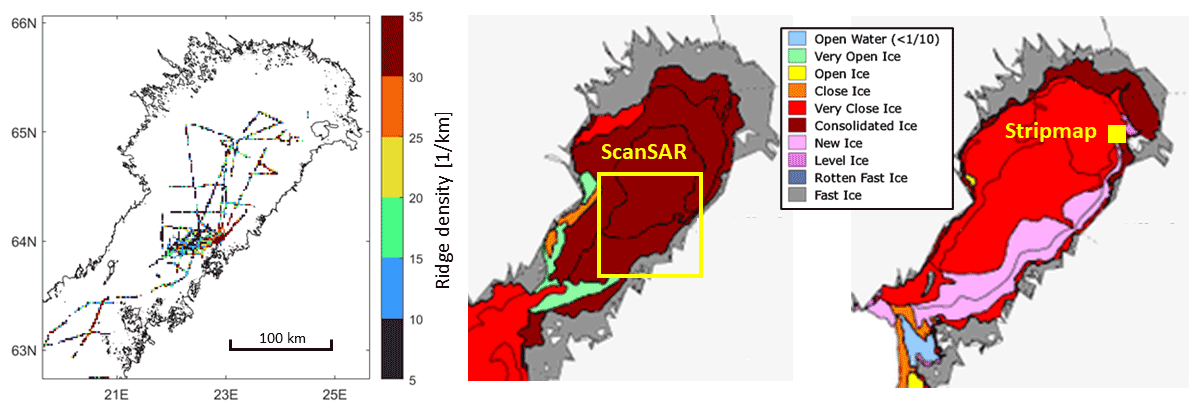
Figure 1 The profiling measurement lines during the 2011 field campaign. The ice conditions on the days of the images.

The ScanSAR swath width is 100 km, and the azimuthal length is 150 km, while in the studies, a 106 × 94 km subimage was used. The image was land-masked and rectified to the Mercator projection with reference latitude 61^∘40^′ N and pixel size 20 m. As the incidence angle range from 29.5 to 38.7^∘ is narrow, no incidence angle corrections were made (Mäkynen et al., 2002), only the calibration of the backscattering coefficient σ^∘.

The stripmap image is a geocoded ellipsoid-corrected (GEC) product without any terrain correction and a spatially enhanced (SE) product designed for the highest possible square ground resolution. The image was rectified to 1.25 m resolution in the Mercator projection. The covered area is about 33.6×42 km² (width × length), from which a 19×19 km² subimage was used in the analyses.

The ice profile dataset comprising 2800 km of the profile was collected during the week after the ScanSAR acquisition. The helicopter-borne system was similar to that described by Haas et al. (2009). Only the lidar surface profile data are used here, while the electromagnetic (EM) ice thickness has been addressed in Ronkainen et al. (2018). The analysis of lidar data followed standard procedures. After a reference-level determination, the local maxima were identified by the Rayleigh criterion that demands that for two successive maxima, the minimum elevation between them must be less than half from either maximum. Otherwise, the shallower one is not counted. The elevation distribution of maxima has a negative exponential tail for values higher than 0.4 m, which was selected as the cutoff elevation. Above the cutoff, the maxima are assumed to be ridge sails. The average sail height and ridge densities are 0.65 m and 11.7 1 km⁻¹, respectively.

The winter prior to the ScanSAR acquisition and profiling campaign was colder than average. During the campaign, SW winds up to 18 m s⁻¹ triggered opening and deformation periods in the Bay of Bothnia, and the drift speed of the research vessel Aranda serving as the campaign base was typically 0.05–0.2 m s⁻¹. The ice thickness varied from 30 to 60 cm in pack ice. The air temperature increased from −10 ^∘C on 24 February to −1.5 ^∘C on 27 February. When the ScanSAR image was acquired, the air temperature was −2.3 ^∘C at the Aranda base. Snow lines measured during 2–4 March had a mean thickness of 8 cm and a standard deviation of 11 cm. About 50 cm thick snow accumulations were often found by ridges, sometimes covering shallower sails. On 3 March, the snow already had some moisture, and the density varied from 200 to 300 kg m⁻³ on level ice and 300–400 kg m⁻³ near ice ridges. It can be assumed that during the ScanSAR acquisition prior to the campaign, the snow was still dry and did not significantly affect the backscattering.

The winter of 2016 was mild, and only the Bay of Bothnia had an ice concentration of 100 %. Recurrent periods of mostly SW wind induced cycles of deformation, opening and freeze-up. Only in the beginning of March did the basin attain a more persistent ice cover consisting of ridged and rafted ice types. On 5 March, the fast-ice thickness in the NE quadrant of the basin was 50–65 cm, the level of ice thickness in the ridged ice pack was 30–50 cm and the air temperature was from −4 to −1 ^∘C. The temperature stayed below 0 ^∘C, and no snowfall occurred during the 10 d before the stripmap SAR image acquisition date when the snow thickness on the mainland was about 30 cm.

2.2 Approach

From the backscattering viewpoint, the principal quantity to describe ridging is the relative area of ice surface covered by ridge rubble (rubble coverage). Curvilinear ridge sails are often visible, having a roughly triangular cross-section and a typical scale of 1–10 m in the across-sail direction and tens to hundreds of metres in the along-sail direction. However, less well defined block accumulations are also understood here as ridging as they contribute to the rubble coverage. Their signatures in surface profiles are also similar to those of curvilinear ridges.

It appears clear that the returns from the ridge rubble dominate the brighter end of the backscattering intensity histogram. The brightness statistics involve a certain uncertainty, however. The histogram depends on the processing of the image aiming for a good visual appearance. A change in ambient conditions may result in quite different intensity histograms for an otherwise unchanged ice cover. Still, an ice-charting expert can typically recognise in both cases the same ridging signatures as these appear persistent and symptomatically nonhomogeneous. The persistence shows up clearly in binary images comprising a certain percentage of bright pixels from the intensity histogram tail. If the percentage is reduced, the ridging signatures become more sparse but tend to retain structural congruence with the non-reduced signatures.

In a way, the objective of the present approach is to provide a statistical foundation for the assessment that the ridging signatures in two SAR images “look the same”. Towards this end, a certain bright-pixel percentage (BPP) is selected with an intensity threshold. For a lower BPP, the selected bright pixels are expected to be predominantly returns from ridge rubble. The spatial variation related to the ridging signatures is described in terms of the bright-pixel number (BPN) in pixel blocks with side length L or equivalently in terms of the bright-pixel coverage (relative area, density) in the blocks. The side length L and the BPP are variable parameters of the BPN approach.

Proper validation data for the BPN approach would consist of ridge rubble topography in square areas with a comparable side length, for example, scanning lidar data over snow-free ice. The extent of such data is limited, however. The validation data, therefore, consist of linear surface profiles from which ridge sails are identified. The profiles are divided into segments of length L, and the ridge sail numbers (RSNs) in the segments are counted. Only those sails are counted that exceed a certain height threshold. The ridge rubble coverage will inherit the RSN statistics that can then be parametrically compared with BPN statistics for concurrent datasets. The segment length L and the sail height threshold are variables of the RSN approach.

As the BPN and RSN approaches are formally analogical, a more theoretical validation exercise seeks to show that they follow the same statistical model. The model is derived by considering how BPN and RSN values change with threshold changes (threshold process). High-resolution (1.25 m) images resolving individual ridge sails are used.

2.3 Estimating ridge rubble coverage

Ridge rubble coverage can be estimated along a linear profile from ridge sail height and ridge density. To provide realistic estimates, the effect of the cutoff sail height used in the profile analysis must be assessed, as well as the application of results reported on the sail width $/$ height ratio, which is noted as $R=w/h$. Considering first the ridge width, the effect of oblique angles of sail crossings must be taken into account. For randomly oriented ridges, the average width is $\mathit{\pi }/\mathrm{2}$ times the perpendicular width (Mock, 1972). The reported R ratios for perpendicular width are usually around 4. However, the measurements typically refer to the highest point of some sail section, while aerial imagery shows that the sail width does not vary as much as the sail height but is rather constant. The results of Lensu (2003) indicate that the highest point of a sail section is typically 2.5 times the average sail height, and thus the average value of R for random sail crossings is about 10. Additionally, the Rayleigh criterion counts certain wider multiple-peak formations as singular ridges. Deformed ice fields also include scattered rubble and other diffuse roughness not accounted for in the estimates. To include the contribution of these, the value R=13 is adopted.

The cutoff sail height affects both ridge density and ridge height. To estimate the cutoff effect, the extrapolation model by Lensu (2003) is applied. It is assumed that the average sail height is representative of the whole dataset and only the variation in ridge density is at issue. For the present lidar profile data with a cutoff height of 0.4 m and an average sail height of 0.65 m, the model provides estimates that the true average height is h_a=0.48 m and that the true densities are 2.0 times the observed density.

Taken together, the ridge rubble coverage (RRC) along a profile is

$$\begin{array}{}\text{(1)}& {\displaystyle \frac{\mathrm{RRC}}{A}}={\displaystyle \frac{\mathit{\pi }}{\mathrm{2}}}\times R\times h_{\mathrm{a}}\times \mathrm{2}\times \mathit{\lambda }\text{(2)}& {\displaystyle }={\displaystyle \frac{\mathit{\pi }}{\mathrm{2}}}\times \mathrm{13}\times \mathrm{0.00048}\times \mathrm{2}\times \mathit{\lambda },\end{array}$$

where all quantities are in kilometres (h_a is average height; λ is observed ridge density). A unit increase in the observed ridge density for 0.4 m cutoff data increases the along-profile rubble coverage by 1.96 %. However, as the interpolation factors are rough estimates, the value 2 % is used instead.

If the profiling flights have crossed an area multiple times in different directions, which for our data was the case for coastal ridge fields near the flight base, the estimate is representative of areal rubble coverage. For a singular crossing, the relationship involves randomness and is generally the more reliable, the larger the considered area is, provided that homogeneity of ridging conditions persists. On the other hand, independent estimates of rubble coverage from SAR or other data can be converted to ridge density interpreted either as an average of multiple crossings or as the probability of finding the said density in a singular random crossing.

2.4 Threshold process

For an idealised SAR image with accurate real-valued intensities, the pixel values can be arranged into strictly increasing order. Starting from an empty image matrix and from the brightest pixel, the pixels of the ordered series can then be added to the matrix one by one. It can then be studied how the probability of the BPN to increase by 1 depends on the pixel block state $<L,\mathrm{BPN}>$ as defined by L, BPN and possibly other descriptors. The probabilities can then be used to formulate recurrence relations, generating finite BPN distributions.

For integer-valued SAR images, the process starts from the BPN values for maximum intensity and proceeds in unit integer steps by adding pixels of subsequent lower intensity. This is designated as the threshold process. The increase probabilities are replaced by increase rates, that is, the relative number of events of unit BPN increase. For RSNs, an analogical process decreases the sail height threshold by small values, starting from a threshold equalling the highest ridge. The increase rates of the threshold process are then interpreted as increase probabilities of an idealised process. This is legitimate if the number of increase events larger than unity is relatively small for each step.

The threshold process is continued to a certain pixel intensity or ridge sail height cutoff, called a target threshold. The derivation of the statistical model is based on the following observation. The intensity or ridge sail height values higher than or equal to the target threshold can be randomly permuted. This changes the increase rates, generating another threshold process. However, the BPN or RSN distribution observed on the target threshold level is the same for both processes. Thus, the new increase rates can be used to generate the observed distribution. The random permutation has the merit of removing the spatial correlations of intensities or sail heights so that the threshold process is reduced to a random deposition process.

2.5 Scale system of distributions

The threshold process and the distribution model are presented for RSN statistics. The case for the BPN is conceptually analogical but involves complications not present in RSN statistics: discreteness of integer data, resolution set by pixel size and L² as the maximum BPN value.

In RSN analysis, surface profile data are divided into segments, and the numbers n of sails in the segments are counted. A discrete distribution k(n_i) for sail number n_i is defined for each scale L_i. If L_j<L_i is a shorter segment, a conditional distribution k(n_j|n_i) is defined. This can be interpreted as the conditional probability of finding n_j sails in an L_j segment nested inside an L_i segment containing n_i sails. The k(n_j|n_i) can also be called downscaling probabilities as it can be used to derive distribution k(n_j) from k(n_i). The approach can be extended to a cascade of scales, constituting a scale system of distributions.

In an ideal threshold process, the sail heights are arranged into a strictly increasing order and added one by one to the segmented profile. Two nested segments with lengths L_i>L_j are considered so that the longer segment L_i is divided into segments with length L_j and L_i−L_j. If the sail is added in the process to the L_i segment, it has a certain probability of being added to each subsegment. This probability must satisfy the additivity condition $P\left(L_i\right)=P\left(L_j\right)+P(L_i-L_j)$. The simplest assumption satisfying the condition is $P\left(L_i\right)\sim n_i+a{L}_i$, which leads to the hypergeometric distribution (Lensu, 2003):

$$\begin{array}{}\text{(3)}& \begin{array}{rl}k\left(n_j\right|n_i)& ={\displaystyle \frac{\left(\begin{array}{c}a{L}_j+n_j-\mathrm{1}\\ n_j\end{array}\right)\left(\begin{array}{c}a{L}_i-a{L}_j-\mathrm{1}+n_i-nj\\ n_i-n_j\end{array}\right)}{\left(\begin{array}{c}a{L}_i+n_i-\mathrm{1}\\ n_i\end{array}\right)}},\\ & n_j=\mathrm{0},\mathrm{1},\mathrm{\dots },n_i.\end{array}\end{array}$$

If $L_i/L_j\gg \mathrm{1}$, then the finite and discrete distribution k(n_j|n_i) is approximated by k(n_j) and k(n_j) is approximated by the negative binomial distribution

$$\begin{array}{}\text{(4)}& \begin{array}{rl}k\left(n_j\right)& =\left(\begin{array}{c}a{L}_j+n_j-\mathrm{1}\\ n_j\end{array}\right)p^{a{L}_j}(\mathrm{1}-p{)}^{n_j},\\ & \text{where}p={\displaystyle \frac{a{L}_j}{a{L}_j+<n_j>}},\end{array}\end{array}$$

and furthermore, if the expected value $<n_j>$ is large, the continuous approximation of Eq. (4) is the gamma distribution:

$$\begin{array}{}\text{(5)}& f\left(n_j\right)={\displaystyle \frac{\mathrm{1}}{\mathrm{\Gamma }\left(\mathit{\alpha }\right)}}{\mathit{\beta }}^{\mathit{\alpha }}{n}_j^{\mathit{\alpha }-\mathrm{1}}{e}^{-\mathit{\beta }{n}_j},\mathit{\alpha }=a{L}_j,\mathit{\beta }={\displaystyle \frac{a{L}_j}{<n_j>}}.\end{array}$$

It is convenient to assume that L_i is a regional scale where ridging statistics are described by the negative binomial k(n_i), as approximated by the gamma distribution. The hypergeometric k(n_j|n_i) is then used to describe local variation.

The statistical model is validated in two stages. First, the additivity condition is validated by conducting a threshold process for selected scales and target thresholds and observing whether the increase rates have a linear dependence on the RSN or BPN. In the next stage, the distribution models are fitted to the data. In the sections to follow, this is done by the observed mean and variance, and the goodness of fit is checked. The parameter a is obtained from the variance

$$\begin{array}{}\text{(6)}& \mathrm{var}\left(n_j\right|n_i)={\displaystyle \frac{L_j{n}_i(a{L}_i+n_i)(L_i-L_j)}{L_i^{\mathrm{2}}(a{L}_i+\mathrm{1})}}\end{array}$$

and

$$\begin{array}{}\text{(7)}& \mathrm{var}\left(n_j\right)=\langle n_j\rangle +{\displaystyle \frac{\langle n_j{\rangle }^{\mathrm{2}}}{a{L}_j}}\end{array}$$

for the hypergeometric and negative binomial models, respectively. The variance for the negative binomial distribution is larger than the mean, which ensures that a is positive in Eq. (7). The parameter a quantifies the relative strength of the component process of the random spatial deposition of sails, that is, the Poisson process. If the validation results agree for test cases selected from a certain scale range, it can be concluded that the scale system is applicable over the scale range.

2.6 Simulation of SAR texture by the threshold process

To analyse the BPN threshold process in full detail requires that bright pixels are added one by one in process steps. For integer-valued images, this cannot be attained. On the other hand, it is possible in a validation approach where the generative hypotheses are tested by simulating the generative process. The simulation commences from a certain stage of the observed threshold process. New bright pixels are added one by one following the assumed probabilities and possibly other conditions. The simulated result is then compared with the observed one.

A binary image with value 1 (white) for an observed low percentage of brightest pixels is used to seed the process. The simulation changes the value of black (zero) pixels into white, one at a time. This is done by a scale cascade, which is assumed here to follow the linear generative hypothesis. The first step divides the image into four rectangles along randomly chosen vertical and horizontal lines. To each rectangle is assigned weight aN0+N1, where N0 is the number of pixels, N1 is the number of white pixels and a<1 is a parameter that controls the relative strength of a random spatial placement (Poisson process). One of the rectangles is selected for the next step with a probability defined as the ratio of the rectangle weight to the sum of weights. The selected rectangle is divided further into 4, and the cascade is continued until the rectangle contains only 1 black pixel that is changed to a white pixel. The process repeats until a preset number of white pixels is reached.

The simulation approach can also be applied to other generative hypotheses. Imposed maps of spatially distributed weights can be used to include spatial aspects of the generative process, like correlations, homogeneity, gradients and support, i.e. the subregion outside of which the process is not active.

3 Results

3.1 Observed threshold process rates and distributions for ridge sail number

From the profile dataset described in Sect. 2.1, profiles exceeding 5 km in length were selected and truncated to be divisible into 1.6 km, in total 2256 km. In RSN analysis the values $(\mathrm{50},\mathrm{100},\mathrm{200},\mathrm{400},\mathrm{800})$ (metres) were used for the segment length L. The threshold process decreased in 0.01 m steps from 2.5 m (10 ridges). The target threshold was set to 0.5 m (18 638 ridges).

The increase rates per step were determined as the mean value of the RSN increases, including zero increase, and the presented results are for the pooled data comprising all steps to the 0.5 m target threshold. The increase rates were calculated both for the original data and for randomly permuted sail heights. The results shown in Fig. 2 disregard the tail part with excessive variation. In the right panel of Fig. 2, the highest RSN values correspond to ridge density 160 km⁻¹, a value characteristic of rubble fields with no level ice visible. The increase rates were linear with a slight superlinear bend.

Figure 2 Sail number increase rate for a threshold process with target threshold 0.5 m. (a) Rate for observed sail heights and randomised sail heights for segment length L=100 m. (b) Rates for randomised sail heights for different segment lengths.

The rates for non-randomised data deviate after beginning from a linear-to-sublinear increase. For other scales, the behaviour was similar, and for long L values, the rate more or less settled to a constant value in its tail part. A likely reason for this is that sail height correlations that arise naturally as block thickness (a parameter controlling ridge sail height) vary spatially during the course of the ice season. Correlations were indeed found between the RSN and the average sail height.

The hypergeometric and negative binomial distributions were fitted to the data with observed mean and variance. The negative binomial k(n_i) agrees well with the empirical distributions derived from the full dataset in Fig. 3. Only the number of empty segments is overestimated for 200 m and 400 m segment lengths. Figure 4 shows the hypergeometric distributions k(n_j|n_i) for the conditioning scale L_i=1600 m and for the range $(\mathrm{50},\mathrm{100},\mathrm{200},\mathrm{400})$ of the subsegment scale L_j. The results for two values of the conditioning RSN, n_i=16 and n_i=72, are shown. These are equivalent to ridge densities 10 and 45 km⁻¹ for the segments L_i. The agreement is good, considering that the subset size is limited by a fixed value n_i. Similar results are found for other combinations of L_i, L_j and n_i.

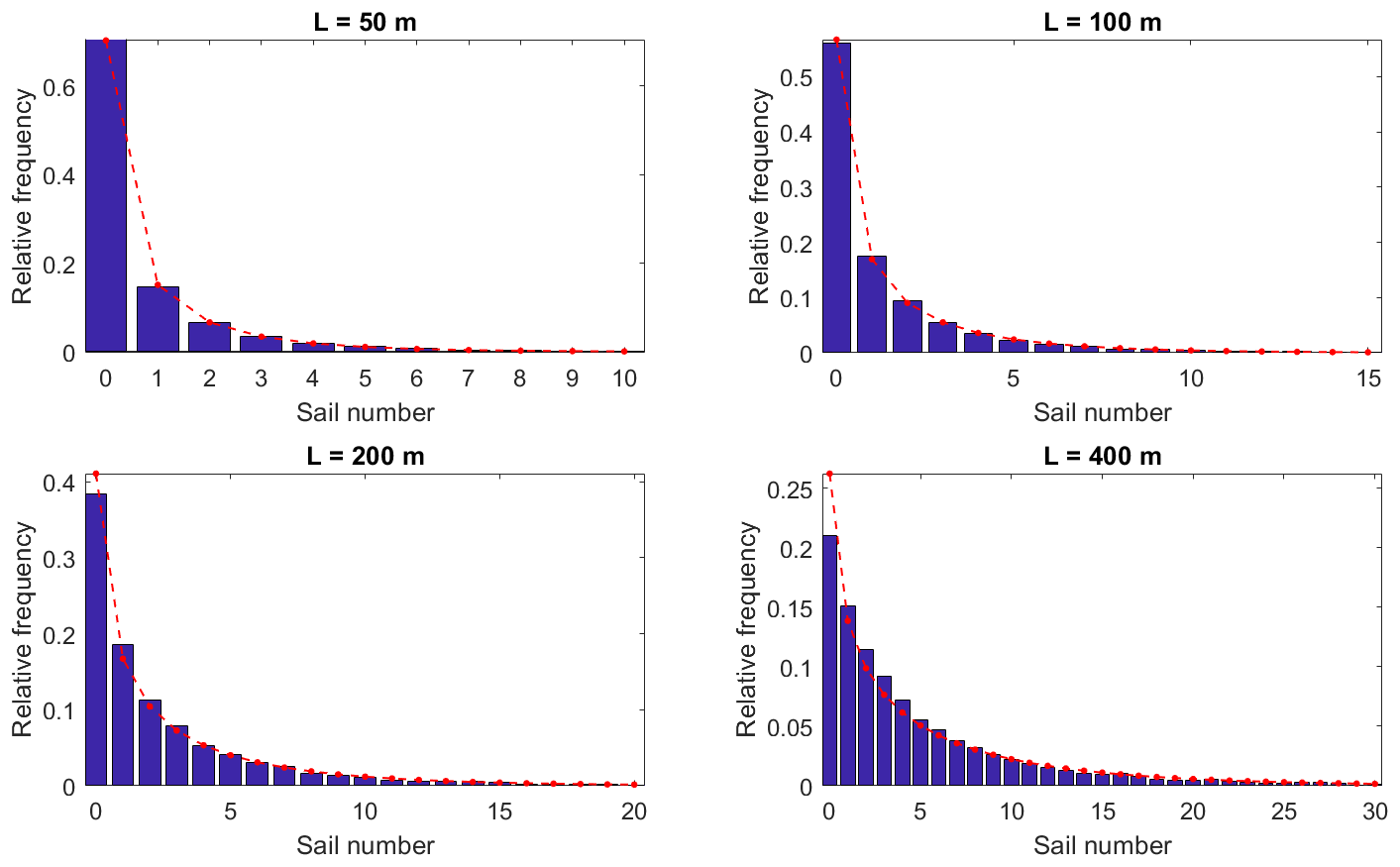
Figure 3 Negative binomial fits to the RSN distribution for the full lidar dataset and for different segment lengths.

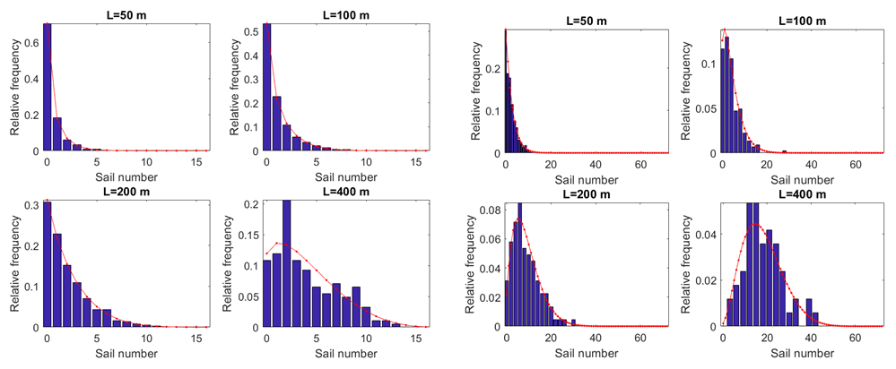
Figure 4 Hypergeometric fits for distributions k(n_j|n_i) conditioned by L_i=1600 m and n_i=16 (left panel group) and n_i=72 (right panel group). The scales L_j belong to $[\mathrm{50},\mathrm{100},\mathrm{200},\mathrm{400}]$.

The hypergeometric model was derived from the assumption that the rate of the RSN increase for the segment length is proportional to n+aL. The parameter a is obtained from the mean and variance and is generally found to decrease with L following the power law. For the hypergeometric case shown, the exponent has about the same value of 0.5 for all values of the conditioning n_i from 16 to 72. The parameter a was interpreted as the relative Poisson intensity, which also provides the rate of sail appearances to empty segments in the threshold process. If there is no rubble present in the segment, it can be said to consist of level ice and cannot experience a change in the RSN from 0 to 1 either. The Poisson parameter of level ice segments is zero, and the observed Poisson parameter a is obtained by multiplying the true Poisson parameter of rubble segments by their relative coverage. Thus the power law suggests that the area covered by ridge rubble has fractal geometry.

3.2 Characteristics of high-resolution SAR

The pixel size of the March 2016 stripmap image is 1.25 m, which resolves backscattering signatures from individual ridges. The size of the image (Fig. 5) is 19 × 19 km, but for analysis and visualisation, different subimages were also used, principally 7000 × 7000 (8.7 × 8.7 km) and 1024 × 1024 (1.3 × 1.3 km) subimages with representative ridging signatures. To proceed following the approach outlined in Sect. 2.2, a certain bright-pixel percentage (BPP) is selected and a binary image with unit values for the bright pixels is generated. The variation in bright-pixel density is described in terms of bright-pixel numbers (BPNs) in pixel blocks with variable side length L.

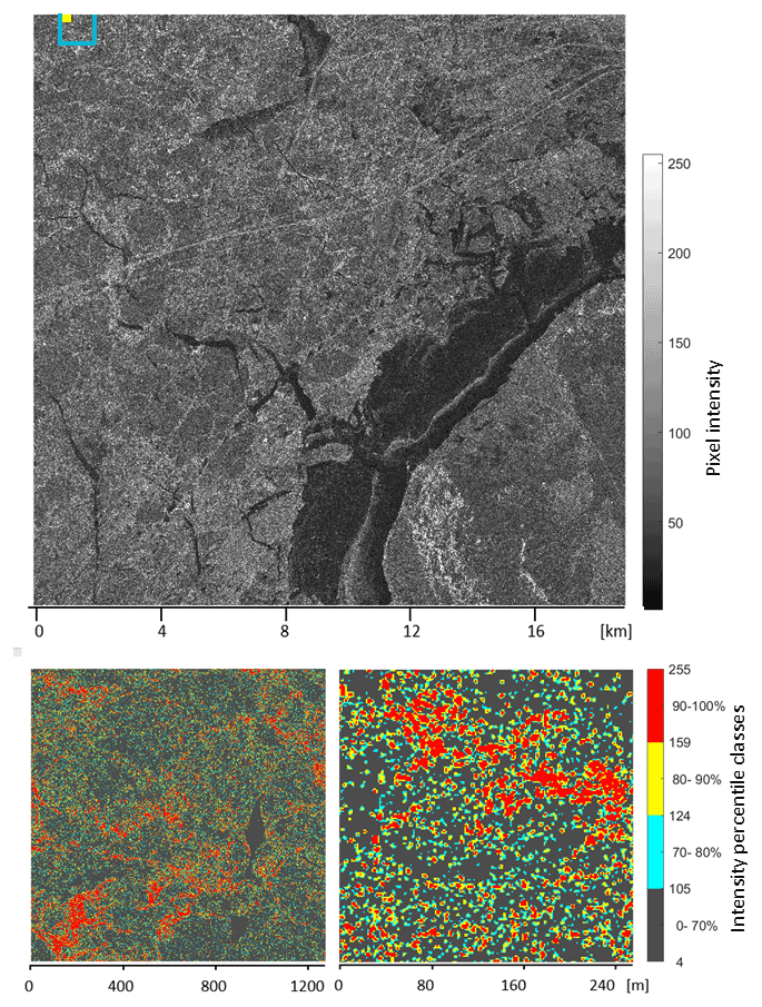
Figure 5 The 15 200 × 15 200 stripmap image with the locations of 1024 × 1024 (blue) and 200 × 200 (yellow) subimages indicated (upper panel). The 1024 × 1024 and 200 × 200 subimages (lower panel).

Two derivative image types are also presented. Following the BPN approach, the first derivative replaces (as a sliding operation) pixel values with BPN values calculated for pixel blocks centred on the target pixel. This is accomplished by a convolution with an L × L all-ones kernel. The result is termed the “contextual image” as the visibility of ridging signatures and their effective resolution depend on BPP and block side length L, which can be chosen to suit the application context. The other derivative is the “category image”, which divides the brightest 30 % of pixels into three 10 % classes, for either the original or the contextual image.

In the category-image version of the stripmap image, Fig. 5, ridging features appear to be visually delineated by the brightest 20 %, while the interval 70 %–80 % begins to add more scattered pixels. The hope of a similar quasi-photorealistic appearance as is found in comparable TerraSAR-X terrestrial images by Dumitru and Datcu (2013) does not quite materialise. There are obvious linear ridges, but these consist of chains of detached bright components that do not connect to continuous features. Larger features, reminiscent of ridge groups or small rubble fields, are more readily observed. However, they are also aggregates of detached bright components, and a similar texture is also found for ship ice channels that are flat and rather uniform beds of bright scatterers. Increasing the bright-pixel percentage from 30 % slightly improves the connectedness of ridge signatures but at the same time obscures their delineation by adding scattered bright pixels to apparent level ice areas.

These observations agree with the results by Manninen (1992) and Carlström and Ulander (1995) that indicate that bright returns from ridge rubble depend on random factors like a favourable orientation of blocks, while the returns from the remaining sail may fail to be clearly distinct from the surrounding level ice. The apparent randomness also corroborates the assumption that the density of the bright pixels in the image is proportional to the coverage of ridge rubble.

In the contextual image and its category-image rendering, Fig. 6, the sliding-block side length is L=101 (126 m), and the BPP is chosen to be 20 %, comprising the red and yellow pixels of Fig. 5. It is seen that the ridging signatures are enhanced and their connectedness improved in the contextual images.

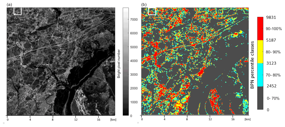
Figure 6 The 15 200 × 15 200 contextual image (a) and corresponding category image (b) derived from the full image with BPP 20 % and sliding-block side length 101. The colour bar extends to the maximum observed BPN in the blocks, 9831. The location of the 1024 × 1024 subimage is also indicated.

3.3 Observed threshold process rates and distributions for high-resolution BPNs

For the analyses, a 7000×7000 upper-left-corner subimage of the stripmap image was used in order to avoid the refrozen lead visible in Fig. 5. The image was divided into non-overlapping pixel blocks with side length L, measured in pixels. The intensity threshold was decreased by unit integer steps, starting from 255, and the rate of BPN increase as a function of the BPN was obtained for each step. In the presented results, the rate data comprise all steps down to the target threshold. In the subimage, 1.2 % of the highest intensities are saturated to 255. This percentage is equal to that for the intensity band [218,254] and would correspond to the extending of the exponential tail of the intensity histogram beyond 255 to 350. This somewhat affects the results for the initial steps of the process.

Analogically to the RSN analysis, the pixel intensities above and including the target threshold were randomly permuted. In Fig. 7, the block side length is set to L=32 and the target intensity threshold values $(\mathrm{182},\mathrm{149},\mathrm{118},\mathrm{86})$ are chosen, corresponding to BPP values $(\mathrm{5},\mathrm{10},\mathrm{20},\mathrm{40})$. As for the RSN, the magnitude of the rates is not relevant, and they have been scaled so that the sum rate equals L² or 1024. The different degrees of saturation then separate the point clouds in the figure. Linearity is observed unless the saturation of the pixel block is felt after three-quarters of the block capacity is filled.

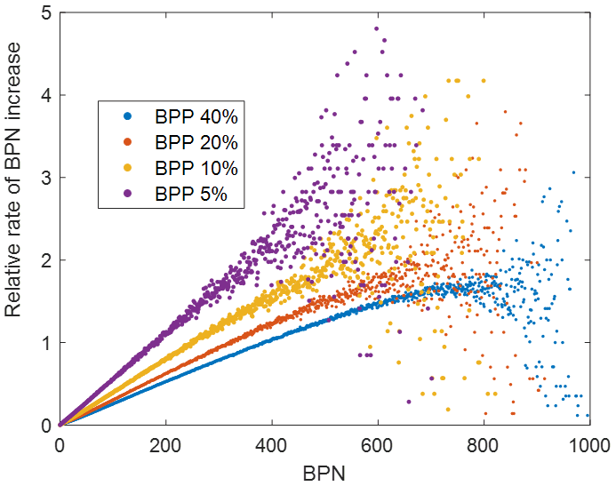
Figure 7 The BPN increase rates for pixel block side length 32 and BPP increasing from 5 % to 40 % in a binary fashion.

In the other test case in Fig. 8, the BPP is set to 20 % (target intensity threshold 118), and the block side length increases from 4 to 128. In addition to the same scaling of rates as in the first test case, the BPN range [0,L²] has been scaled to [0,1]. The results are similar to the first test case. For comparison, the same result is shown for the original data where the pixel intensities are not randomised. For higher L, the relationship is then approximately linear for small relative BPN values, but otherwise, it is quadratic. Intensity correlations are the likely reason for this, but no further conclusions are attempted.

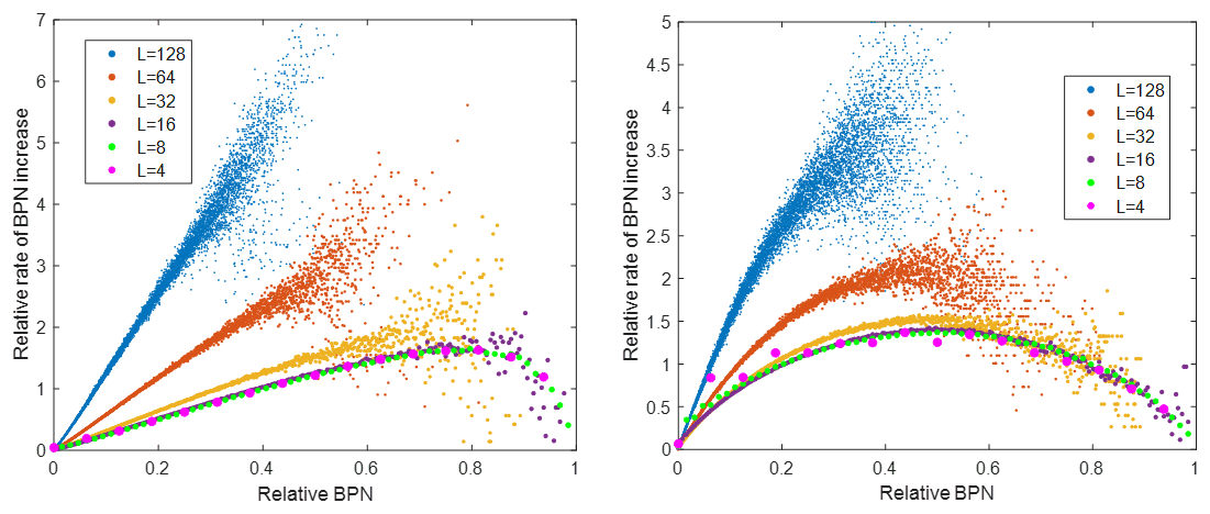
Figure 8 The BPN increase rates for BPP 20 % and the pixel block side length increasing from 4 to 128 in a binary fashion for randomised data and for original data.

The agreement of the proposed distribution system with the data is again good. Distributions were calculated from block tiling of the 9216×9216 (11.5×11.5 km) upper-left-corner subimage. Figure 9 shows negative binomial distributions k(n) fitted by observed mean and variance for BPP 10 %, and three scales are shown. The fourth subplot shows the model parameter a as obtained from the mean and variance for the binary cascade of scales $L=\mathrm{8},\mathrm{16},\mathrm{\dots },\mathrm{256}$ and for three BPP values. The power law exponents vary from −0.45 to −0.37 and are thus close to but somewhat smaller than the values obtained in the RSN analysis. Also, the negative hypergeometric model k(n_j|n_i) conditioned by scale L_i and BPN value n_i applies well. Figure 9 shows the results for selected combinations of L_i, L_j and n_i. The conditioning scale cannot much exceed the value L_i=16 as the number of instances n_j for conditioning pairs (L_i,n_i) decreases with increasing L_i as $L_i^{-\mathrm{4}}$.

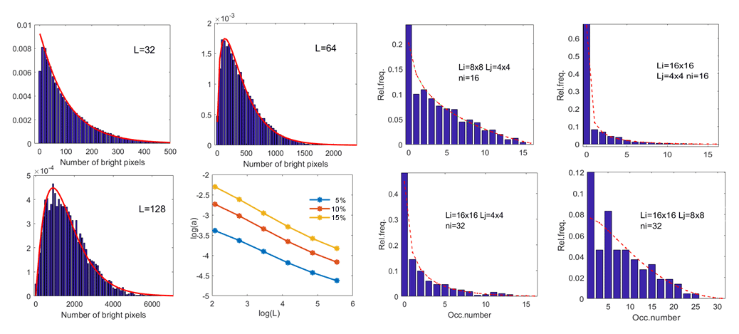
Figure 9 In the left panel group are BPN distributions and their negative binomial fits for BPP 10 % and three different pixel block side lengths L. The parameter a is also shown for a scale cascade $\mathrm{8},\mathrm{16},\mathrm{\dots },\mathrm{256}$ and for three different BPPs. In the right panel group are hypergeometric fits for conditional BPN distributions for different combinations of conditioning scale L_i and conditioning BPN n_i.

3.4 Simulated high-resolution SAR texture

The simulation algorithm was applied to the 1024 × 1024 subimage indicated in Fig. 5. The white pixels of the initial binary image correspond to BPP 3 %. The simulation added 10 % so that the resulting BPP is 13 %. If aN0≫N1, the Poisson process dominates the simulation step, but overall, the process gravitates towards image areas with a higher density of white pixels. However, if the fraction of white pixels is initially low, the Poisson component process tends to add nonzero pixels into larger empty areas, first creating dispersion and then spurious clusters. To reduce this, an additional condition requires that in a process step, a white pixel cannot be added within a rectangle if its fraction of nonzero pixels is below a threshold C_o and the rectangle area measured as a pixel number is within certain limits [N1,N2]. This effectively means restricting the support of the process.

The parameters were $a=\mathrm{1}/\mathrm{20}$, $C_o=\mathrm{1}/\mathrm{100}$ and $[N\mathrm{1},N\mathrm{2}]=[\mathrm{100},\mathrm{20}\mathrm{000}]$, and the results are shown in Fig. 10. Although not matching exactly on the pixel level, both 13 % images exhibit the same pixel density variations. For contextual and category images for L=21, the results for the real and simulated 13 % images match almost exactly; that is, they contain the same information at scale L=21. The results provide additional corroboration for the soundness of the generative hypothesis. They also provide the insight that certain parts of “non-deformed” ice should be left outside the ridging statistics, a feature also previously suggested by the emergence of power law exponents for the parameter a in the distribution fits. The parameters of this demonstration were determined by simple experimentation, but more systematic approaches can be conceived. Especially, intensity values could be incorporated, which would introduce spatial intensity correlations, and the fractality suggested by the distribution analysis could be encoded into the simulation steps.

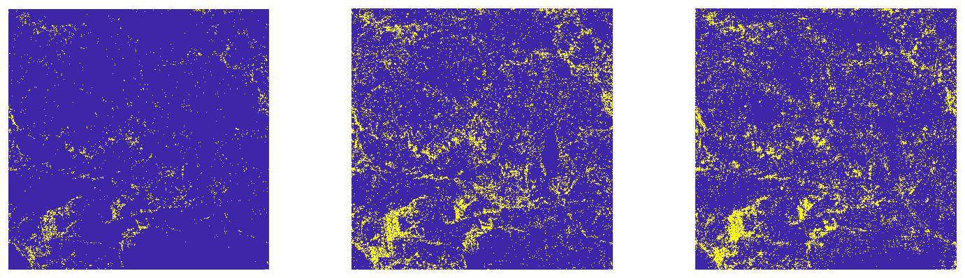
Figure 10 BPP 3 % binary image, BPP 13 % image, and the BPP 13 % image generated from the BPP 3 % image by the simulation algorithm.

3.5 SAR and lidar comparison for the 2011 image

The analysis of ridged areas in the 20 m resolution TSX ScanSAR image proceeds in a similar manner to the analysis of high-resolution SAR data. The basic SAR tools are the bright-pixel percentage (BPP) and the counting of bright-pixel numbers (BPNs) in pixel blocks. The target is distributions f(x), where x is the estimated ridge rubble coverage (RRC) in pixel blocks (SAR RRC) or their ground truth counterparts as determined from lidar surface-profiling flights (lidar RRC).

The essential assumptions are that lidar RRC can be estimated from profile data, Sect. 2.3; that the bright-pixel number can be used as a proxy for SAR RRC also for 20 m resolution data; and that both RRC concepts inherit their statistics from the model for RSNs and high-resolution SAR BPNs, Sect. 3.1 and 3.3. It is noted that the 20 m resolution can still detect much of the ridging signature in Fig. 11 and that the simulation method described in Sect. 2.6 works.

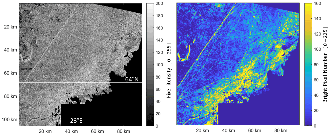
Figure 11 The test area covered by the TSX SAR imagery with resolution of 20 m. On the right is the contextual image with BPP 20 %.

The BPP is set to 20 %. The exact BPP value is not essential, but the chosen one is expected to comprise most of the ridging signatures and not too much level ice. Similarly, as for the high-resolution image, the bright pixels are mostly not connected to continuous ridging features. A convolution operation is then conducted, generating a contextual image, Fig. 11, where each pixel value of the original image is replaced by the number of bright pixels (BPNs) in a 15-by-15-pixel block centred at the pixel. As the target is rubble coverage, the BPN values are changed to percentage points. The convolution operation acts similarly to the high-resolution SAR and effectively reveals the ridged areas and connects many of the ridging structures that are only vaguely discernible in the original SAR imagery.

For comparisons between the SAR RRC and lidar RRC, the resolution of the contextual image is weakened to 1 km². This coarser-scale image, Fig. 12, is called an analysis image, and its pixel value is the mean of all pixels inside the corresponding contextual-image pixel block. These pixels represent the SAR RRC and are compared with lidar RRC values determined in grid cells matching the pixels with respect to size and location. The lidar data were assigned to the grid cells in Fig. 12 using the coordinates included in the data. If the lidar grid cell contains data, its value is the ridge density detected in it, and the RRC in percentage points is estimated by multiplying the density by 2 %, Eq. (5). Ridge densities larger than or equal to 50 then have 100 % RRC. This was the case for about 2 % of all the cells with nonzero ridge density and occurred only in the rubble field zone close to the eastern coast.

Figure 12 The analysis image over the test area presented as a SAR RRC image (a) and the corresponding lidar RRC image (b). The units are percentage points in both images.

As mentioned in Sect. 2.1, ice drift and deformation occurred during the profiling campaign week after the acquisition of the SAR image. As the ice drift could have been well over 10 km during the time gap and the flights are from several days, it is not possible to establish a pairing between the two RRC estimates in SAR analysis pixels and lidar grid cells, and the comparison was made regionally. All lidar data in the area covered by the SAR image were used for the RRC values in the lidar grid, Fig. 12. The SAR RRC analysis image, Fig. 12, includes all pixels outside the mask (N=7549 pixels). Lidar data (N=1017 cells) comprise about 13 % of the SAR pixels.

The two datasets are compared in terms of a quantile–quantile (Q–Q) plot for the respective distributions. This can be viewed as a nonparametric approach to comparing their underlying distributions. There is also no need to compare the grid values pairwise or have equally sized datasets. The quantile pairs are largely located along a line with a ratio of 1.34 between the quantiles (Fig. 13, the left panel). This indicates that the shapes of the distributions are similar and that they may belong to the same distribution family. As lidar RRC is expected to follow a gamma distribution (Eq. 5), this is then also expected for SAR RRC. For two gamma distributions, the linearity of the Q–Q plot entails that the shape parameters are equal, which also holds for the model (Eq. 5) if the scale L_j and the process parameter a are the same for both. The slope of the Q–Q plot then equals the ratio of the scale parameters, suggesting that a value of 1.34 can be used as a scaling coefficient.

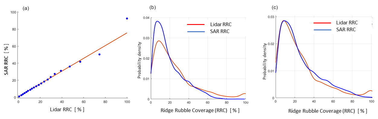
Figure 13 The quantile–quantile plot for the SAR and lidar datasets (a). The SAR and lidar RRC distributions overlaid (b). The scaled SAR and original lidar RRC distributions (c).

It was examined how close to each other the distributions of the SAR and lidar RRC are with and without the scaling coefficient of 1.34, Fig. 13. The original SAR and lidar RRC densities show the same basic shape but do not match well. When SAR RRC is scaled by 1.34, the match is improved, and the obtained mean values are very close to each other: 26.2 % for the scaled SAR RRC and 25.9 % for the lidar RRC. Converting these RRC values back to ridge density values yields about 13 km⁻¹ for both datasets. Gamma distributions were also fitted to both datasets. The maximum likelihood estimates for the shape parameter of the scaled SAR RRC gamma density is 1.7 and the scale parameter 15.5. The respective values for lidar data are 1.4 and 18.2. Thus, although the parameters of the fits are close to each other, they are not equal.

The problems with the fit and agreement with gamma distribution mostly concern the tail part of the distribution. The linearity of the Q–Q plot was no longer valid for SAR RRC over 50 % and for lidar RRC over 75 % RRC. The SAR RRC values over 50 % are relatively rare in the data, and highly ridged areas form proportionally a much larger fraction in the lidar data. Especially the rubble field hump seen at the end of the lidar distribution is not present in the SAR distribution. As the lidar flights frequently flew over the large coastal rubble field zone (Fig. 11), a larger proportion of the lidar data were collected from this area than was the case with the SAR RRC data. The scaling coefficient was found to increase with the area of SAR included in the comparison and varied from 1.3 to 1.6. With a spatially more uniform coverage of the lidar flights over the SAR image, the agreement would probably have been better for the tail part.

As expected, decreasing the BPP value increases the scaling coefficient when the SAR image extent and the lidar data stay fixed. Three cases were examined: for BPP 10 %, the scaling is 2.22; for 15 %, it is 1.61; and in the above analysis with BPP 20 %, it is 1.34. In all three cases, the Q–Q plot is linear for its main part and the mean of the scaled SAR RRC distribution is always close to the lidar RRC mean.

3.6 Contextual images as ridging information

Although in SAR images from a ridged ice cover the bright returns are predominantly from ridge rubble, the step to quantitative methods has proved hard. The bright pixels do not typically connect well to ridging features but appear as diffuse pixel clouds. The connectivity is improved in the contextual images that enhance the ridging signature by a BPN sliding operation (Fig. 6 or Fig. 11). If the BPP is changed, the BPN values change accordingly, but for a random pair of pixel blocks the change more often retains the size order of their BPN values than reverses it. Consequently the appearance of the contextual image is not sensitive to changes in BPP. This is more strikingly demonstrated in the category versions of the contextual images (Fig. 6).

The upper panels in Fig. 14 show the 1024 × 1024 subimage of the high-resolution SAR indicated in Fig. 5 and its BPP 20 %, L=21 contextual derivative presented as a category image in the upper right panel. However, for the BPP range from 2 % (pixels with value 255) to 95 %, the category image would be almost identical to that in the upper right panel. The same result is found for several alternative methods to generate a contextual image, like the L=21 sliding-block average of intensity. Moreover, the information of the contextual image is essentially retained in different randomising transformations. In the lower left panel of Fig. 14 the 1024 × 1024 image has been multiplied 8 times by a random matrix that erodes the ridging signature almost beyond visual recognition. However, the contextual category image still emerges essentially unchanged in its main features in the right panel.

Figure 14 Results for 1024 × 1024 stripmap subimage multiplied 8 times by a random matrix. (a, c) The subimage (a) and the randomised subimage (c). (b, d) Category versions of contextual images obtained by BPP 20 % and a 21 × 21 convolution kernel for the original subimage (b) and for the randomised subimage (d).

The observed behaviour is due to the fact that changes in BPP, changes in method or randomising operations on average preserve the order of values in the contextual images. This feature is enhanced in the category versions as the flux of values across category boundaries is then relatively small. This can be studied in detail by pixel-to-pixel mapping between two contextual images. For the 1024 × 1024 subimage and L=21 pixel block, the pixel-to-pixel mapping of 20 % BPN values to intensity averages is monotonous on average. For each BPN value, the mapped intensity averages have a normal distribution with a standard deviation in the range of 3.5–4.5. On the other hand, the widths of the 70 %–80 %, 80 %–90 % and 90 %–100 % categories for the intensity average are 9, 15 and 102, respectively. Thus, the highest class, in particular, retains its delineation in this method change. More importantly, if the change in BPN values induced by a change in ambient conditions preserves the order on average, the category images can be consistently used in the daily production of ice information.

The pixel block side length L affects the resolution of detail in the contextual images, and its value may be chosen to suit the context, hence the term. Including a pragmatic viewpoint, L=21 of Fig. 14 and L=101 of Fig. 6 correspond to the width and length scales of ice-breaking ships so that the BPN values of contextual images provide the number of bright scatterers that the ship bow or the whole ship interacts with at a time. As the BPN has been shown to be a proxy for ridge rubble coverage, the contextual images have direct pertinence to navigability. The categorised versions can be interpreted as classes of navigational difficulty or as a delineation of areas that a ship should not enter. They can be used in tactical navigation or in route optimisation that only seeks to avoid difficult ice types. More advanced route optimisation is based on physical models for the added resistance from the ridges. The ice-going speed and the probability of besetting can then be obtained in simulations that take the ice conditions along alternative tracks as input, specifically ridge density and ridge height (Kuuliala et al., 2016). As the contextual images provide only relative ridge density estimates, the scaling to true values, as well as ridge height, must be determined by other means. These may include observations from ships; measurements; or satellite data, especially ICESat-2 profiles. Another possibility is to use a ship’s response, observed remotely from AIS (Automatic Identification System) data for ship speeds and positions, to classify the contextual-image signatures directly in terms of ice cover resistance (Similä and Lensu, 2018).

4 Discussion and conclusions

Ice-charting experts are usually able to recognise the same ridging signatures in SAR images that have different resolutions or are taken in different ambient conditions. The present approach proceeded from this observation by analysing SAR images in terms of the local density of bright pixels chosen by a certain percentage (BPP). The tail intensity variations, which are often relied on in SAR ice type classification approaches, were left to play a secondary role. The quantification is in terms of bright-pixel numbers (BPNs) counted in pixel blocks. First, high-resolution images for which the bright returns can be assumed to come from individual ridge sails were investigated. A distribution model was derived and found to also apply to ridge sail numbers (RSNs) determined for surface profile segments. A validation study using a medium-resolution SAR image with near-concurrent ground truth data demonstrated that the method can be used to derive ridge density up to the scaling factor. This can be provided by independent observations, most promisingly by ICESat-2 surface profiles.

The distribution model was derived with a threshold process where bright pixels or ridge sails were deposited sequentially onto the image canvas or surface profile. The probability for the deposition to select a certain pixel block or profile segment was proportional to the corresponding BPN or RSN value. This raises the question of the role of the physical ridge formation events in profiling segments that manifest as the formation of new sails or as the appearance of new bright scatterers in a SAR image time series. An alternative approach to sail statistics considers sail spacings or sail-to-sail distances. A new sail divides the spacing into two shorter spacings, and if the probability of this happening does not depend on the spacing, the spacing distribution is asymptotically lognormal, as shown by Kolmogorov (1941). As the RSN and the number of spacings are about equal for ridge segments, the probability that a new ridge appearing in the profile ends in a certain segment is then proportional to the RSN of the segment. This indicates that the applicability of lognormal and that of hypergeometric models have the same physical origin. The lognormal has also been found to apply to sail spacings in the Baltic since Lewis et al. (1993). Another hint of the background physical process is that the BPN statistics are parameterisable by pixel block side length L rather than area L². The length of ridge sails typically exceeds L, and thus a ridge formation event does not add bright scatterers pixel-wise but as a chain crossing the pixel block.

In the high-resolution SAR, it was likely that most bright pixels indicate ridge rubble. Their statistics were studied using binary images, and no attempt was made to interpret the intensity variations in the bright pixels, although it may be noted that they followed exponential distribution. It was observed that the bright-pixel texture in dense ridge fields was not much different from that of ship channels that are flat rubble beds. All studied BPP values generated more or less the same contextual images. This suggests that the correlation between sail height and SAR intensity is weak. It remains to be investigated whether connectedness, curvature and other measures may provide ridge height estimates.

High-resolution SAR data provide a kind of baseline for the investigations on ridge parameter retrieval as the returns have a connection both with ground truth ridging statistics and with the backscattering models by Manninen (1992) and Carlström and Ulander (1995). The hypergeometric model provides a scale connection tool that can be used to study how lower-resolution pixel intensities relate to the pixel statistics in higher-resolution matching-pixel blocks. Our high- and medium-resolution images did not have the required spatiotemporal overlap unfortunately. However, the medium-resolution image did not appear much different in binary BPP versions, which mostly consisted of disconnected pixels and generated contextual images that enhanced the ridging features in a similar way for a wide range of BPP values. Also, the simulation algorithm applied to the medium-resolution image as well as the gamma distribution asymptotics of the hypergeometric model.

Relying on the results obtained in Mäkynen and Hallikainen (2004) for the scatterometer data at the X- and C-band and Dierking (2010) for L-band SAR imagery, it can be hypothesised that the results for the C-band and L-band would follow similar lines. A possible obstacle to the presented analysis occurs when the air temperature is warm enough to make the snow cover wet. As shown by Mäkynen and Hallikainen (2004), this essentially decreases the contrast between level and deformed ice, and thus it is uncertain whether the proposed method applies in the wet snow conditions. However, for this not to happen, any change in ambient conditions should severely overturn the order of BPN values; otherwise the persistence of contextual category images demonstrated in Sect. 3.6 would prevail. In addition, higher ridges are often snow-free and less affected by wet conditions. Further studies applying matching multiplatform data with different resolutions and varying ambient conditions are needed to clarify this and other unanswered issues left open.