Effects of topographic and meteorological parameters on the surface area loss of ice aprons in the Mont Blanc massif (European Alps)

Ice aprons (IAs) are part of the critical components of the Alpine cryosphere. As a result of the changing climate over the past few decades, deglaciation has resulted in a surface decrease of IAs, which has not yet been documented, except for a few specific examples. In this study, we quantify the effects of climate change on IAs since the mid-20th century in the Mont Blanc massif (western European Alps). We then evaluate the role of meteorological parameters and the local topography in the behaviour of IAs. We precisely mapped the surface areas of 200 IAs using high-resolution aerial and satellite photographs from 1952, 2001, 2012 and 2019. From the latter inventory, the surface area of the present individual IAs ranges from 0.001 to 0.04 km². IAs have lost their surface area over the past 70 years, with an alarming increase since the early 2000s. The total area, from 7.93 km² in 1952, was reduced to 5.91 km² in 2001 (−25.5 %) before collapsing to 4.21 km² in 2019 (−47 % since 1952). We performed a regression analysis using temperature and precipitation proxies to better understand the effects of meteorological parameters on IA surface area variations. We found a strong correlation between both proxies and the relative area loss of IAs, indicating the significant influence of the changing climate on the evolution of IAs. We also evaluated the role of the local topographic factors in the IA area loss. At a regional scale, factors like direct solar radiation and elevation influence the behaviour of IAs, while others like curvature, slope and size of the IAs seem to be rather important on a local scale.

1 Introduction

The predicted shift in climate dynamics over the next decades will undoubtedly have severe consequences on the high mountain environments, primarily on glacier extent (Rafiq and Mishra, 2016; Kraaijenbrink et al., 2017; IPCC, 2021), permafrost (Magnin et al., 2017) and ice and snow cover (Rastner et al., 2019; Guillet and Ravanel, 2020). The effects of climate change on glaciers constitute a remarkably well-discussed topic in the scientific community (Yalcin, 2019).

Meteorological parameters (mainly temperature and precipitation) are the main driving forces responsible for these changes (Scherler et al., 2011; Bolch et al., 2012; Davies et al., 2012). Shifting temperature and precipitation trends lead to the advance or retreat of glaciers both in volume and surface area (Liu et al., 2013; Yang et al., 2019). On a regional and global scale, many authors have studied the impacts of climate warming on glacier retreats and, consequently, on the hydrology of the mountain environments (e.g. Baraer et al., 2012; Sorg et al., 2014; Frans et al., 2016; Coppola et al., 2018).

However, as observed by Furbish and Andrews (1984), Oerlemans et al. (1998), Hoelzle et al. (2003), and Salerno et al. (2017), glaciers present in the same climate regime can respond to climate change in different ways. The local climate variations can partly explain these variable responses. However, many of these variations result from different morphometric (size, shape, length) and topographic (altitude, slope, aspect, curvature, terrain ruggedness) characteristics.

Several studies have been devoted to understanding the linkage between topographic factors and the response of glacier/ice bodies (e.g. Davies et al., 2012; De Angelis, 2014; Salerno et al., 2017).

The World Glacier Monitoring Service (WGMS) monitors glacier changes in all the major mountain regions of the world. However, most mapping and monitoring studies on a global scale focus on massive glaciers since they are generally assessable and easier to monitor compared to other ice features (Liu et al., 2013).

Studies are rare for small glaciers or ice bodies, which generally show a more pronounced response to climate change (Oerlemans and Reichert, 2000; Triglav-Čekada and Gabrovec, 2013; Fischer et al., 2015). This has led to a critical gap in our understanding of their behaviour and mass balance estimates. As part of this trend, ice aprons (IAs), sometimes also referred to as “rock faces partially covered with ice” (Gruber and Haeberli, 2007; Hasler et al., 2011), have also received poor attention from the scientific community.

These small ice accumulations on steep rock slopes are commonly found in all significant glacierized basins worldwide. However, a concrete and well-summarized definition for IAs is still missing from the literature. Previously, many authors like Benn and Evans (2010), Singh et al. (2011), and Cogley et al. (2011) tried to define IAs, but the most precise definition for IAs up to now can be found in Guillet and Ravanel (2020) for the Mont Blanc massif (MBM; European Alps). These authors defined IAs as “very small (typically smaller than 0.1 km² in extent) ice bodies of irregular outline, lying on slopes >40^∘, regardless of whether they are thick enough to deform under their weight”. The small spatial extent of the IAs makes them very difficult to map and monitor. Also, they are typically present in extremely challenging topographies on isolated steep slopes. Cogley et al. (2011) specified that IAs are “lying above the head of a glacial bergschrund which separates the flowing glacier ice from the stagnant ice, or a rock headwall”.

Because of their presence on steep slopes, IAs are essential natural elements for the practice of mountaineering, especially in famous destinations like MBM (Barker, 1982). IAs are passing points for many classic mountaineering routes (Mourey et al., 2019). Hence, the loss of IAs is a severe threat to the iconic practice of mountaineering, inscribed in 2019 by UNESCO on the Representative List of the Intangible Cultural Heritage of Humanity. IAs on steep rock walls also carry the critical role of covering steep rock slopes and preventing them from direct exposure to direct solar radiation, thus partly preventing the warming of the underlying permafrost. In addition, a recent study by Guillet et al. (2021) showed that the ice present at the base of the Triangle du Tacul IA could be older than 3 ka, making IAs a potentially important glacial heritage.

Guillet and Ravanel (2020) showed that IAs in the MBM have lost mass since the Little Ice Age (LIA). Based on six different IAs, their study also showed an acceleration in the shrinkage since the 1990s. They linked the loss of IA area with meteorological parameters, mainly air temperature and precipitation. It was thus the first documented evidence that IAs have been losing ice volume due to the changing climate. However, since this study was local and based on only a few IAs, the authors could not consider other factors, such as the local topography critical for small glacier bodies (Hock, 2003; Laha et al., 2017).

Thus, to overcome these limitations, we propose a large-scale analysis to ascertain the relationship of the area loss of IAs with the meteorological parameters, mainly air temperature and precipitation, using a more comprehensive database (ca. 200 IAs) covering the whole MBM. The large inventory of IAs has been surveyed thanks to high-resolution aerial and satellite images from 1952, 2001, 2012 and 2019. Further, based on our inventory, we also evaluate the impacts of the topographic/geometric controls on the area changes of IAs. For this, we consider the size of IA, elevation/altitude, slope, curvature, topographic ruggedness index (TRI), direct solar radiation and permafrost conditions (classified together as topographic factors) based on past studies on similar themes (e.g. Oerlemans et al., 1998; Warren, 2008; DeBeer and Sharp, 2009; Jiskoot et al., 2009; Davies et al., 2012; Salerno et al., 2017).

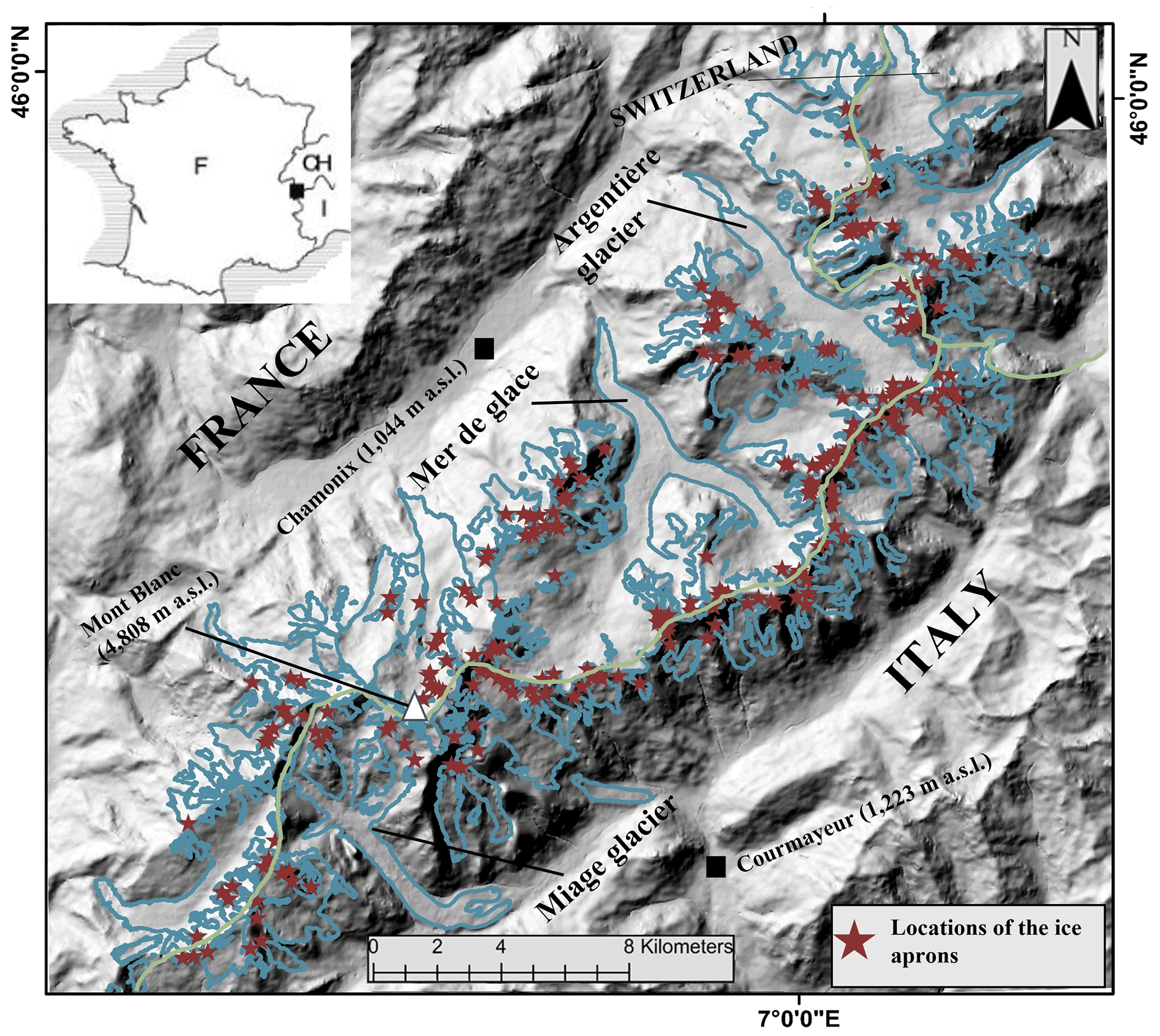
Figure 1 The Mont Blanc massif (western European Alps). A total of 200 IAs (red stars) were digitized accurately on high-resolution images. The glacier outlines (in blue) come from Gardent et al. (2014). The green line shows the border between France, Italy and Switzerland.

2 Study area and the impacts of climate change in the region

The Mont Blanc massif (Fig. 1) is located in the north-western (external) Alps between France, Switzerland and Italy. It covers ca. 550 km² and displays some of the highest peaks in the European Alps; a dozen peaks have elevations greater than 4000 m a.s.l. The MBM thus shows a significant variation in the elevation range throughout the massif; the lowest point of the massif is at 1050 m a.s.l. (Chamonix), and the highest, the top of Mont Blanc, is at 4808 m a.s.l.

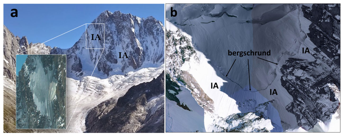
Figure 2 Ice aprons and their locations in the MBM: (a) IAs on the N face of Grandes Jorasses (4208 m a.s.l.), photograph courtesy Ludovic Ravanel, and (b) IAs on the headwall of the Argentière glacier separated by a bergschrund (3280 m a.s.l.), IGN orthophotos 2015.

Because of its high elevation, the MBM is also the most glacierized massif in the French Alps (Gardent et al., 2014). There are about 100 glaciers often bordered by steep rock walls, including 12 glaciers larger than 5 km². The steep and irregular terrain facilitates the development of many unique ice bodies like cold-based hanging glaciers or IAs. Figure 2 shows two examples of the locations of the IAs on the steep N faces from the study region.

As a result of an asymmetry of the massif, six of the largest glaciers are located on its NW French side, where slopes are gentler than the Italian side and glaciers are well fed by the westerly winds while melting is reduced by the protection of the shaded north faces. The SE Italian side is characterized by smaller glaciers and generally steeper slopes bounded by very high sub-vertical rock walls. This asymmetry is also evidenced by the difference in the meteorological conditions observed on the two sides of the massif. For example, the mean annual air temperature (MAAT) recorded in Chamonix (at 1044 m a.s.l.) is +7.2 ^∘C, while that in Courmayeur (1223 m a.s.l.) is +10.4 ^∘C (Deline et al., 2012). Comparing the annual MAAT values from 1934 to today shows that MAAT increased by >2.1 ^∘C in Chamonix (Météo-France data). Moreover, the increase in MAAT from 1970 to 2009 was almost 4 times faster than from 1934 to 1970 (Mourey et al., 2019). The MAAT also increased by 1.4 ^∘C not only at lower elevations but also at elevations exceeding 4000 m a.s.l. between 1990 and 2014 (Gilbert and Vincent, 2013). The MBM has experienced nine summers characterized by heatwaves (where maximum temperatures for at least three consecutive days exceed a heatwave temperature threshold defined for the region) since 1990 (1994, 2003, 2006, 2009, 2015, 2017, 2018, 2019 and 2020), with the one as recent as 2018 being the second (after 2003) hottest. The average annual precipitation recorded for Chamonix is 1288 mm, and that for Courmayeur is 854 mm (Vincent, 2002). The precipitation rates in the MBM have remained relatively constant since the end of the LIA, but there is a noticeable decrease in the number of snowfall days relative to the total precipitation days below 2700 m a.s.l. (Serquet et al., 2011).

Global warming has led to a general retreat trend of the MBM glaciers since the end of the LIA despite small re-advances culminating in 1890, the 1920s and the 1980s (Bauder et al., 2007). The recorded loss of glacier surface area was 24 % of the total area from the end of the LIA to 2008 (Gardent et al., 2014). The reported loss of ice thickness is also noteworthy. For example, the loss of ice thickness at the front of the Mer de Glace glacier (1650 m a.s.l.) from 1986 to 2021 is 145 m; the Argentière glacier (1900 m a.s.l.) has lost 80 m in thickness from 1994 to 2013 (Bauder et al., 2007). At 3550 m a.s.l., the surface of the Géant glacier also lowered by 20 m between 1992 and 2012 (Ravanel et al., 2013). The glacier retreat and shrinkage concur with the equilibrium line altitude (ELA) that rose by 170 m between 1984 and 2010 in the western Alps (Rabatel et al., 2013). As a result of the loss of ice volume, the density of open crevasses has considerably increased, along with an increase in bare ice areas. In some instances, ice volume loss leads to instability of steep slopes, and serac falls from the front of warm and cold glaciers are more frequent (Fischer et al., 2006). This latter process can be typical during the warmest periods of the year (Deline et al., 2012). Warming trends also intensify moraine erosion, resulting in an increase in rockfall and landslide events (Deline et al., 2015; Ravanel et al., 2018). Degradation/warming is another critical concern for permafrost (e.g. Haeberli and Gruber, 2009).

3 Data description

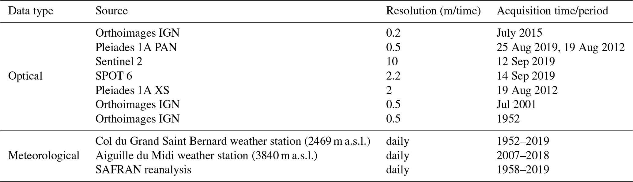
This section describes all the datasets obtained from diverse sources used in this study (Table 1).

Table 1 Datasets used for the study.

3.1 Digital elevation model

Since one of the main aims of our study was to perform a joint analysis of the behaviour of small ice bodies and the local topography, it was paramount to have a robust high-resolution and accurate digital elevation model (DEM) for the study region. To avoid the uncertainties that most global DEMs are plagued with and to overcome the problem of different DEM origins on the French and Italian sides of the MBM, we built our own DEM. As part of the CNES Kalideos Alps project, stereoscopic sub-metre resolution optical images from the Pleiades constellation were acquired. Using the pair of stereo panchromatic images (25 August 2019), a 4 m resolution DEM was computed using the Ames Stereo Pipeline (ASP), an open-source processing chain developed by Shean et al. (2016). The parameters used for the processing were kept the same as those of Marti et al. (2016). The second part of the processing involved accurately co-registering the newly built DEM with an existing reference DEM of high precision and accuracy. For this purpose, we used the automatic DEM co-registration methodology given by Nuth and Kääb (2011). To co-register the source 4 m Pleiades DEM (Fig. 3a) we used a 2 m lidar DEM for the area around the Argentière glacier (8×2.5 km spatial extent) (Fig. 3b) built by the Institut des Géosciences de l'Environnement (IGE). A precisely co-registered, high-resolution, robust 4 m DEM was obtained at the end of the processing steps. More detailed information about the processing parameters for DEM generation and co-registration can be found in Kaushik et al. (2021). We used this DEM to compute topographic parameters like slope, aspect, curvature, elevation, TRI, mean annual rock surface temperature (MARST) and direct solar radiation.

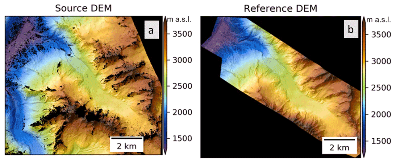
Figure 3 (a) The source Pleiades DEM used for further analysis; (b) the reference lidar DEM of the Argentière glacier used for co-registration.

3.2 Optical aerial and satellite images

This study relies on high-resolution aerial and satellite images (Table 1). Working with data from different sources allowed us to tap into the wealth of data for comparison. Spanning over seven decades and covering the entire MBM, orthoimages for 1952, 2001 (0.5 m resolution) and 2015 (0.2 m resolution) were downloaded from Géoportail IGN (French Institut national de l'information géographique et forestière), while the panchromatic and XS images from SPOT 6 and Pleiades at 2.2 and 0.5 m respectively were downloaded from the Kalideos Alps website. Considering the small dimensions of the ice bodies, we could only work with high-resolution optical images covering the entire MBM. We were thus limited by only one set of excellent quality images for 1952 and 2001, as very high-resolution images for this study period were unavailable from any other source. Hence our mapping exercise relied only on the orthoimages for these two time periods. For 2012 and 2019, we had data from multiple sources (Pleiades, SPOT and orthoimages) to deal with the problems associated with the lack of coverage, cloud cover, illumination, shadow and seasonal snow cover that made visual interpretation difficult. We used a combination of Pleiades and SPOT 6 XS images for mapping the IA boundaries, with validation of results conducted with the help of the orthoimages. To avoid overestimating the extent of IAs, we utilized images acquired at the end of the summer period (late August or early September). Considering that our optical images came from many sources, it was necessary to accurately co-register all images. We used the automatic image-to-image co-registration tool in ENVI 5.6. The process included locating and matching several feature points called tie points in a reference image and a warped image selected for co-registration. Here, we used the Pleiades panchromatic image of 2019 as a reference, and all the warped images were accordingly co-registered. Both coarse and fine co-registration procedures were performed, and the co-registration process was stopped when the RMSE values achieved were less than half the pixel resolution of the warped image based on the recommendations of Han and Oh (2018). A more detailed description of the co-registration process was discussed in Kaushik et al. (2021).

3.3 Meteorological data

Proxies to define accumulation and ablation phases were built to explore the correlated variations in the surface area of IAs with the changing climate. A similar study for six IAs was performed by Guillet and Ravanel (2020); we aim to test the validity of their results with a more extensive database (ca. 200 IAs) in the entire MBM. Since the IAs are spread across different elevation ranges, we tested the results using the SAFRAN reanalysis product (Vernay et al., 2019) that produces gridded temperature, precipitation, wind speed, and other datasets of meteorological variables at an hourly time step. These data were available as NetCDF files from 1958 for all the French massifs; at elevation belts every 300 m; at 0, 20, and 40^∘ slopes; and for all eight aspects (N, NE, E, SE, S, SW, W, NW). Our study is based on two different meteorological datasets described in the subsections below to compare the differences.

Figure 4 SAFRAN reanalysis product temperature time series from 1952–2019 for different elevations in the MBM. The figure shows the variation of the mean annual temperatures for the entire study period.

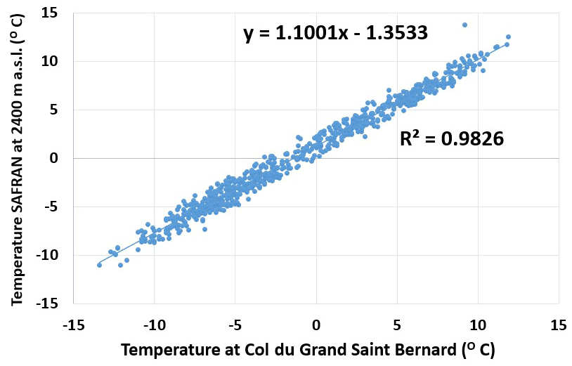
Figure 5 Correlation between the monthly averaged temperature measurements at the Col du Grand Saint Bernard (GSB) and the SAFRAN reanalysis data at 2400 m a.s.l.

3.3.1 Meteorological datasets used by Guillet and Ravanel (2020)

The first part of our analysis follows a similar methodology followed by Guillet and Ravanel (2020) in their analysis. Like their study, we used homogenized weather records from the Col du Grand Saint Bernard (GSB), located close to the MBM at 2469 m a.s.l. and provided by MeteoSwiss and from the Aiguille du Midi (AdM) cable car station (3810 m a.s.l.). GSB represents a similar climatological regime to the MBM, and the weather records were available for an extended period starting from the 1860s. Such long-term weather records were unavailable from any weather station in the MBM. Since all IAs are located at elevations above the elevation of the GSB weather station, it was necessary to transform the weather records to an elevation closer to the average elevation range of the IAs. For this reason, it was necessary to transform the data from the GSB station using the weather records from the AdM weather station (data available since 2007). Guillet and Ravanel (2020) found a strong correlation between the monthly averaged AdM and GSB temperature records and were able to transform the GSB temperatures using a linear model:

$$\begin{array}{}\text{(1)}& T_{\mathrm{AdM}}=\mathit{\alpha }{T}_{\mathrm{GSB}i}+\mathit{\beta }+r_i,\end{array}$$

where α=0.87 (slope), $\mathit{\beta }=-\mathrm{7.7}$ ^∘C (intercept) and r (residuals) has zero mean.

No transformation for the precipitation values was performed as this relation is tough to establish and not always linear (Smith, 2008). Hence, the original GSB precipitation values were used for the analysis. Using these weather records, Guillet and Ravanel (2020) found a robust correlation between ablation and accumulation proxies and the surface area change of six IAs. We used the same datasets to test for similar potential relationships for ca. 200 IAs, and the results are shown in Sect. 5.3.

3.3.2 Meteorological datasets used in this study for comparison

Since the study from Guillet and Ravanel (2020) involved a small number of IAs, the disparity arising from elevation differences of IAs (in turn, the temperature and precipitation coming from weather stations at a fixed elevation) could have been minimized or not well represented. We decided to use the SAFRAN reanalysis product and checked for similar potential relationships of climate variables with the surface area change of IAs. The first problem we encountered was that the SAFRAN data starts from 1958, while our first images date from 1952. Therefore, for comparison, it was essential to interpolate the missing data for the 6 years before 1958 (Fig. 4). Like the previous methodology, we looked for a linear relationship between the SAFRAN temperature data (at 2400 m a.s.l. elevation belt) and the GSB temperature data. We again found a strong correlation between the two datasets (Fig. 5) which helped us transform the data using

$$\begin{array}{}\text{(2)}& T_{\mathrm{SAFRAN}\mathrm{2400}}=\mathit{\alpha }{T}_{\mathrm{GSB}i}+\mathit{\beta }+r_i,\end{array}$$

where α=1.01 (slope), $\mathit{\beta }=-\mathrm{1.35}$ ^∘C (intercept) and r (residuals) has zero mean.

For the SAFRAN data estimated (2400 m a.s.l.) from 1952, we extrapolated the data for all elevation bands. We used a standard gradient of −0.53 ^∘C (100 m)⁻¹ increase in elevation based on the observations of Magnin et al. (2015) for the MBM.

As previously stated, a similar relationship for precipitation was tough to establish. Hence, for the analysis, we used the SAFRAN precipitation data from 1958 and extrapolated the precipitation values from the GSB weather station to all elevation bands of SAFRAN data before 1958 (6 years up to 1952). However, taking a cue from the previous study of Guillet and Ravanel (2020), we expect this impact to be insignificant when considering the results over seven decades.

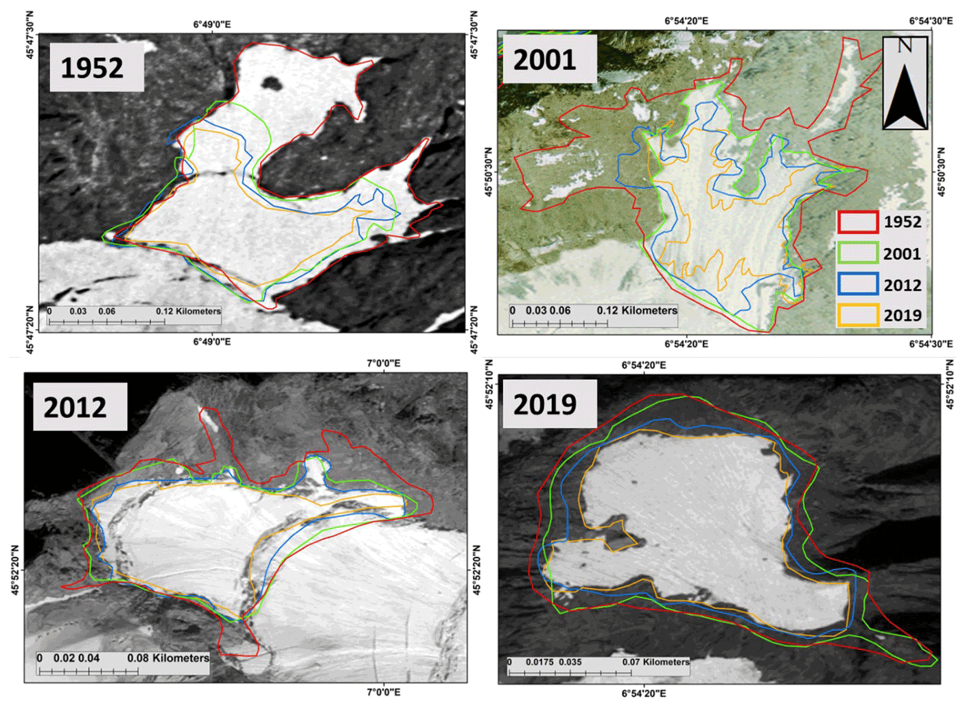
Figure 6 IA extent delineated on high-resolution images: (a) orthophotos 1952, (b) orthophotos 2001, (c) Pleiades panchromatic 2012 and (d) Pleiades panchromatic 2019. The different coloured polygons represent the surface area for each date. The orthophotos are courtesy of the IGN, while the Pleiades images were acquired as part of the CNES Kalideos Alps project.

4 Methods

4.1 Mapping the surface area of IAs from high-resolution satellite images

IA boundaries were manually delineated/digitized by the first author of this paper to maintain data consistency in a geographic information system (GIS) environment for 1952, 2001, 2012 and 2019. The problem of seasonal snow, which can lead to an overestimation of surface areas, was avoided using images at the end of the ablation period. The differentiation of IAs from other snow/ice bodies relies on the slope angle (we only consider ice bodies on slopes >40^∘ to be IAs) and whether they are thick enough to deform under their own weight and show movement, like in the case of hanging glaciers. The slope mask to remove areas with slopes <40^∘ was built in ArcGIS 10.6 using the Pleiades DEM. Figure 6 shows the variations in the surface areas of IAs over the study period. It also highlights the importance of high-resolution images because of the small dimensions of our studied ice bodies. However, these data are not always available in the best quality for the past periods as we could only very accurately map 200 IAs (out of the total 423 IAs reported in Kaushik et al., 2021) for all the periods. These 200 IAs were selected carefully after a detailed visual inspection and considering issues related to shadow and illumination. Since a point-based correlation analysis (with meteorological and topographic parameters) requires very high accuracy and precision of mapping, any significant uncertainty would have resulted in a major bias in our correlation estimates. To avoid this, we used only 200 of the best mapped IAs for the correlation analysis. However, for the estimation of the total area of IAs in 1952, 2001, 2012 and 2019, as described in Sect. 5.2, we use the complete database of 423 IAs with the assumption that overall, for the entire database, the uncertainty in the mapping (± the surface area) cancels out eventually and becomes insignificant.

4.2 Generation of topo-climatic parameters

The relative area loss of IAs for three time periods, i.e. 1952 to 2001, 2001 to 2012, and 2012 to 2019, is analysed with all topographic factors. The area loss is expressed as a relative percentage of the area lost between the first observation and the next. Authors like Salerno et al. (2017) have also used absolute values, but for our study, this would not give a fair estimation for the analysis as it generates a bias based on the size of IAs. The factors we considered for our analysis are elevation, slope, aspect, curvature, TRI, direct solar radiation (all estimated in ArcGIS 10.6), MARST and size of the IAs. The topographic parameters are generated using the 4 m Pleiades DEM described in Sect. 3.1.

4.2.1 Direct solar radiation

Direct solar radiation (DSR) measures the potential total insolation across a landscape or at a specific location. On a local scale, components such as topographic shading, slope and aspect control the radiation distribution (Olson and Rupper, 2019). For estimating the DSR, the viewshed algorithm was run based on a uniform sky and a fixed atmospheric transmissivity value of 1. Mahmoud Sabo et al. (2016) showed the application of these algorithms in areas of rough topography. The total DSR (DSR_tot) for a given location is calculated as the sum of the DSR (Dir_θ,α) from all the sun sectors (calculated for every sun position at 30 min intervals throughout the day and month for a year):

$$\begin{array}{}\text{(3)}& {\text{DSR}}_{\mathrm{tot}}=\sum {\text{DSR}}_{\mathit{\theta },\mathit{\alpha }}.\end{array}$$

The direct solar radiation (Dir_θ,α) with a centroid at zenith angle (θ) and azimuth angle (α) is calculated using the following equation:

$$\begin{array}{}\text{(4)}& \begin{array}{rl}{\text{DSR}}_{\mathit{\theta },\mathit{\alpha }}& =S_{\mathrm{Const}}\cdot \left({\mathit{\beta }}^{m\left(\mathit{\theta }\right)}\right)\cdot {\text{SunDur}}_{\mathit{\theta },\mathit{\alpha }}\\ & \cdot {\text{SunGap}}_{\mathit{\theta },\mathit{\alpha }}\cdot \cos \left({\text{AngIn}}_{\mathit{\theta },\mathit{\alpha }}\right),\end{array}\end{array}$$

where S_Const is the solar constant with a value of 1367 W m⁻²; β is the transmissivity of the atmosphere (averaged over all wavelengths) for the shortest path (in the direction of the zenith); m(θ) is the relative optical path length, measured as a proportion relative to the zenith path length; SunDur_θ,α is the time duration represented by the sky sector; SunGap_θ,α is the gap fraction for the sun map sector; and AngIn_θ,α is the angle of incidence between the centroid of the sky sector and the axis normal to the surface.

The final map of DSR is the sum of values calculated at an hourly time step for every pixel, as per the resolution of the DEM used. The values of solar radiation are given in watts per square metre (W m⁻²). Higher values for solar radiation indicate higher insolation, while lower values suggest low insolation. We prefer DSR over the aspect for our analysis to avoid bias due to local shading on sun-exposed faces, considering the slope angle associated with the aspect.

4.2.2 Elevation

Elevation strongly influences the meteorological conditions within the same region, significantly altering the precipitation, temperature and wind regime even at a local scale. Generally, higher elevations receive more precipitation and experience lower temperatures and higher wind speeds. Hence, regions at higher elevations, especially above the ELA, should favour more accumulation than ablation. However, wind-driven snow at higher elevations does not readily accumulate on steep slopes. Some IAs may take advantage of the leeward conditions at lower elevations and sustain for more extended periods. Similar results for large glaciers have previously been reported by Bhambri et al. (2011) or Pandey and Venkataraman (2013).

4.2.3 Mean slope

Slope angle strongly influences ice velocities of glaciers, the mass flux and the hydrology of the mountain environments. Its influence on avalanche transport of snow over the glacier surface has been discussed previously (e.g. Hoelzle et al., 2003; DeBeer and Sharp, 2009). Numerous studies have also reported that slope is the single most crucial terrain parameter that controls glacier responses to climate change (Furbish and Andrews, 1984; Oerlemans et al., 1998; Jiskoot et al., 2009; Scherler et al., 2011). In mountainous regions, the terrain slope strongly influences snow accumulation. On steep slopes, accumulation in the temperature range of −5–0 ^∘C can accumulate on steep slopes. Slope likewise plays a key role when calculating other terrain parameters and indices.

4.2.4 Mean annual rock surface temperature

MARST estimates the average annual temperature of the rock surface governed mainly by the potential incoming solar radiation (PISR) and the mean annual air temperature (MAAT). The method for estimating MARST is described by Boeckli et al. (2012) and Magnin et al. (2019). The estimation is based on a multiple linear regression model with the form

$$\begin{array}{}\text{(5)}& Y=\mathit{\alpha }+{\sum }_{i=\mathrm{1}}^k\mathit{\theta }i{X}^i+\mathit{\epsilon },\end{array}$$

where Y is the value for MARST, α is the intercept term, θiXⁱ represents the model's k variables (PISR and MAAT) and their respective coefficients, and ε is the residual error term distributed equally with the mean equal to 0 and the variance σ²>0. For predicting the values of MARST in steep slopes, we use the equation

$$\begin{array}{}\text{(6)}& {\text{MARST}}_{\left(\mathrm{pred}\right)}=\mathit{\alpha }+\text{PISR}\cdot b+\text{MAAT}\cdot c,\end{array}$$

where α is the MARST_pred value when PISR and MAAT are equal to 0, and b and c are the respective coefficients of PISR and MAAT at measured rock surface temperature (RST) positions. These coefficients were calibrated by Boeckli et al. (2012) (rock model 2) for the entire European Alps using a set of 53 MARST measurement points. The MAAT of the 1961–1990 period was used to calculate MARST, representing a steady state.

The values for MARST are calculated in ^∘C and, for our study region, range from −12 to 10 ^∘C.

MARST is also an important criterion to check for the very likely presence of permafrost below the IAs, which likely allows the formation and existence of IAs.

4.2.5 Topographic ruggedness index

The topographic ruggedness index (TRI) measures the ruggedness of the landscape. TRI was calculated based on the methodology proposed by Sappington et al. (2007). It is calculated as a three-dimensional dispersion of vectors (x, y, z components) normal to the grid cells considering the slope and aspect of the cell. The magnitude of the resultant vector in a standardized form (vector strength divided by the number of cells in the neighbourhood) measures the ruggedness of the landscape. Higher values of TRI thus suggest a more rugged and sporadic terrain, which could block the downward movement of the snow and subsequently lead to the formation of a weak layer, destabilizing the snowpack and leading to small avalanches resulting in mass wasting (Schweizer, 2003). Since IA surfaces are smooth, the TRI values calculated at the surface of the IA are always low. Hence, we consider the TRI values by taking a buffer of 20 m around the IA boundary delineated for the first observation (1952). The mean TRI value from this buffer is considered for our analysis.

4.2.6 Curvature

Curvature, estimated as a second derivative of the surface, defines the shape of the slope. Curvature is considered an essential factor because it can define snow accumulation or ablation rates for a surface. Generally, two types of curvature profiles are known, plan and profile. For our analysis, we only used the profile curvature as it defines the shape of the slope in the steepest direction. From a theoretical point of view, erosion processes prevail in convex (negative values) profile curvature locations, while deposition is predominant in concave (positive values) profile curvature locations. The curvature values define how strongly the slope is convex (lower negative values) or concave (higher positive values). That is why curvatures can be considered essential in the accumulation and ablation rates of a glacier or ice body. Like TRI, the IAs tend to show flat curvature profiles if we consider their surface. Hence, we estimate the curvature values around the same buffer as the TRI and use this for further analysis.

4.3 Proxies for ablation and accumulation

To eventually correlate changes in surface area of IAs with the changing climate, we use the temperature and precipitation data from the transformed GSB weather records and SAFRAN reanalysis product (see Sect. 3.3) to build proxies for accumulation and ablation. The proxy for ablation was built by estimating the annual sum of positive degree days (PDD) computed from the normal probability distribution centred around the mean monthly temperature. Estimation of the PDD is based on the empirical relation, which states that the melting rate is proportional to the surface air temperature excess above 0 ^∘C. Several methods for estimating PDD have been proposed by Braithwaite and Olesen (1989), Braithwaite (1995), and Hock (2003). However, the method proposed by Calov and Greve (2005) also accounts for stochastic variations in temperature during the computation of PDD. The formula for the estimation of the PDD using this method is given by

$$\begin{array}{}\text{(7)}& \mathrm{\text{PDD}}=\underset{\mathrm{0}}{\overset{A}{\int }}\mathrm{d}t\left[{\displaystyle \frac{T_{\mathrm{ac}}^{\mathrm{2}}}{\surd \mathrm{2}\mathit{\pi }}}\exp \left(-{\displaystyle \frac{T_{\mathrm{ac}}}{\mathrm{2}{\mathit{\sigma }}^{\mathrm{2}}}}\right)+{\displaystyle \frac{T_{\mathrm{ac}}}{\mathrm{2}}}\text{erfc}\left(-{\displaystyle \frac{T_{\mathrm{ac}}}{\surd \mathrm{2}\mathit{\sigma }}}\right)\right].\end{array}$$

T_ac is the annual temperature cycle (monthly mean temperatures estimated in ^∘C for the entire year); σ is the standard deviation of the temperature from the annual cycle, A=1 year; and erfc is the conventional error function built into all programming languages.

After computing the PDD, we calculate the cumulative PDD (CPDD) by taking the sum of all the annual PDD values for each observation period (i.e. 1952–2001, 2001–2012 and 2012–2019). This value of CPDD is then used as a proxy for ablation (Braithwaite and Olesen, 1989; Vincent and Vallon, 1997).

The calculation of the proxy for accumulation is more tricky because we only consider the yearly sum of precipitation occurring at a temperature between −5 and 0 ^∘C, as only snowfall within this temperature range is believed to accumulate/adhere to steep slopes (Kuroiwa et al., 1967; Guillet and Ravanel, 2020; Eidevåg et al., 2022). The temperature-dependent indicator function can be written in the following form:

$$\begin{array}{}\text{(8)}& {\mathit{\chi }}_i(T,(t\left)\right)=\left\{\begin{array}{ll}\mathrm{1}& \text{ if }-\mathrm{5}{}^{\circ }\text{C}\le T\left(t\right)\le \mathrm{0}{}^{\circ }\mathrm{C}\\ \mathrm{0}& \text{ otherwise}\end{array}\right..\end{array}$$

4.4 Surface area model

Using the proxy for ablation and accumulation, Guillet and Ravanel (2020) proposed a surface area model to estimate the differences in the surface areas of IAs between different time steps due to the time-integrated changes in meteorological parameters. The main goal is to look for a potential linear relationship between climate variables and the changes in surface areas of IAs, using a multivariate regression model. The equation for the model can be written as

$$\begin{array}{}\text{(9)}& \begin{array}{rl}{S}_{\mathrm{m}}\left(t\right)=S\left(t_{\mathrm{0}}\right)& -\underset{\mathrm{to}}{\overset{t}{\int }}(\mathit{\alpha }\mathrm{1}\text{CPDD}\left(t\right)\\ & -\mathit{\chi }i\left(T\left(t\right)\right)\mathit{\alpha }\mathrm{2}A\left(t\right))\mathrm{d}t+\mathit{\beta }+\mathit{\epsilon }(t),\end{array}\end{array}$$

where S_m(t) corresponds to the modelled surface area at time t; similarly, CPDD(t) and A(t) represent the proxies for ablation and accumulation; S(t=0) is the first available measurement; α1 and α2 are the coefficients of linear regression, β is the intercept, and ϵ the residual. χ(T,t) accounts for precipitation occurring in the [−5, 0 ^∘C] temperature range and is given by the temperature-dependent indicator function given in Eq. (8). The area of IAs at each time step was calculated using the surface area model (with the temperature and precipitation proxies), and we hereafter refer to this area as the modelled area. The measured area is the surface area we delineated using high-resolution optical images.

4.5 Uncertainty estimations

Since this study uses data from different sources and periods, uncertainties of different origins might have been introduced to delineate the IA boundaries. A good estimation of these uncertainties is thus crucial to have a fair estimation of the significance of the results (Racoviteanu et al., 2008; Shukla and Qadir, 2016; Garg et al., 2017). Some sources of uncertainty in this study could arise from (1) errors inherent to the aerial images and satellite-derived datasets, (2) errors resulting from inaccurate co-registration of data from various sources, (3) errors produced while generating the high-resolution DEM from stereo images, and (4) conceptual errors linked with defining the boundaries of IAs in all images. Quantifying the errors inherent in processing all datasets used is challenging, and this is out of the scope of this paper. A detailed accuracy assessment of the DEM generation and co-registration process is provided in Sects. 5.1 and 3.1, respectively. Quantifying errors resulting from the manual delineation of IA boundary is also challenging, but we have previous guidelines from Paul et al. (2017) for the quality and consistency assessment of manual delineations.

One way to assess the area uncertainty is to perform multiple digitizations of the same surface and calculate the mean area deviation (MAD), taking the first digitization as a reference (Meier et al., 2018). Considering this, the first author performed three digitizations for 50 IAs on images from 1952, 2001, 2012 and 2019, considering different challenges associated with aerial and satellite images like shadow and illumination. MAD provides a percentage estimate of how the final area calculated varies across multiple digitizations for each polygon. MAD values are affected by the size of the polygon manually digitized. Previously, authors like Paul et al. (2013), Fischer et al. (2014) and Pfeffer et al. (2014) have reported an increase in the uncertainty of manual digitizations with a decrease in the size of the polygons. With this in mind, we also digitized IAs of different sizes ranging from 0.001 to 0.01 km².

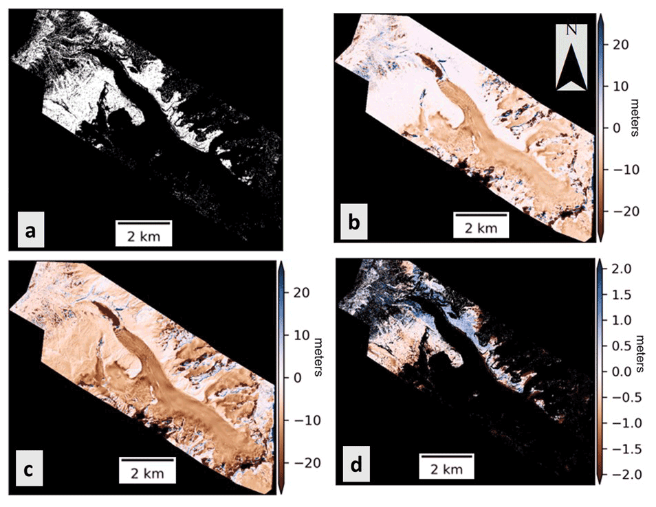
Figure 7 Stepwise Pleiades DEM accuracy assessment: (a) the surfaces used for coregistration, (b) elevation difference before coregistration, (c) elevation difference after coregistration considering all areas and (d) elevation difference after coregistration considering only the stable areas.

5 Results

5.1 Accuracy of the DEM

Figure 7a shows the stable surfaces (after eliminating glacier boundaries, trees and forests) we used for our co-registration process, and Fig. 7b displays the difference in elevation between the reference DEM and the source DEM before co-registration. Figure 7c presents the results after the co-registration process considering all the surfaces (stable and non-stable), and Fig. 7d shows the difference considering only the stable areas after masking out non-stable areas using the glacier boundaries provided by the Randolph Glacier Inventory (RGI v6.0) (Consortium, 2017). The source DEM was translated using the corresponding shift values $x=-\mathrm{5.03}$ m, y=6.00 m and z=3.22 m.

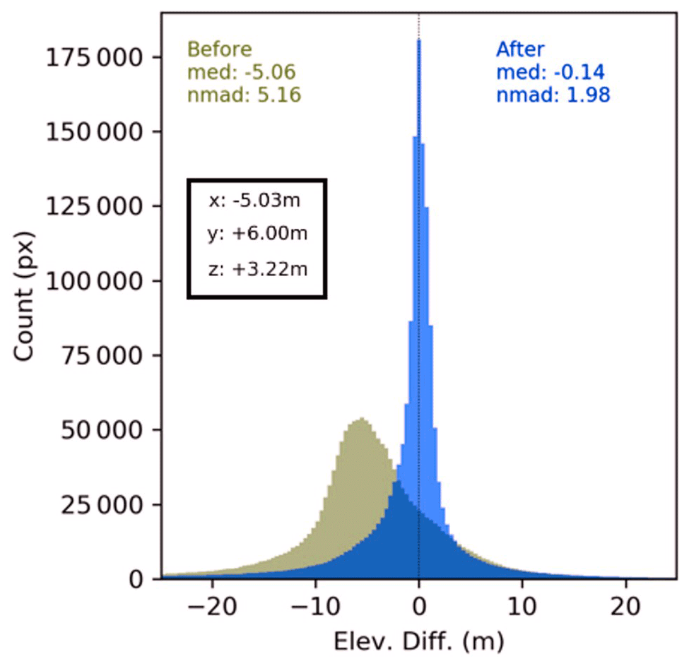
Figure 8 DEM error (elevation difference between the reference and source DEM) distribution for stable areas.

The distribution of errors can be visualized by a histogram of the sampled errors, where the number of errors (frequency) within certain predefined intervals is plotted (Höhle and Höhle, 2009). Figure 8 shows the histogram of the errors Δh (elevation difference between the reference and source DEM) in metres for the stable areas. The accuracy estimates before and after the co-registration are shown by the normalized median absolute deviation (nmad) and the median value calculated together. As can be seen, the nmad and median values before the co-registration process for stable areas were 5.16 and −5.06, respectively. After the co-registration process, the value dropped to 1.98 for the nmad and −0.14 for the median value. This suggests a good correlation between the high-resolution lidar DEM used as a reference and the Pleiades DEM we built.

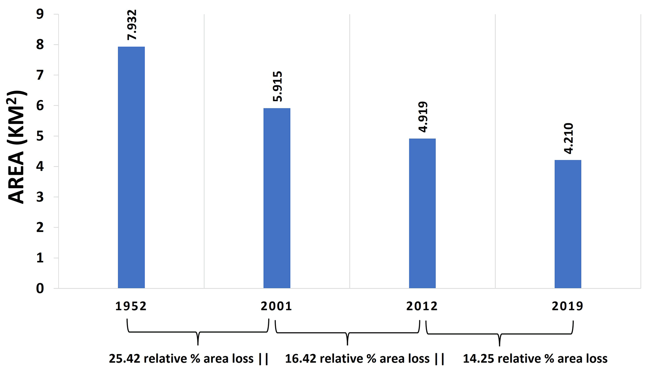
Figure 9 A comparison of the total surface area of all IAs (423 IAs) in the MBM over 67 years.

5.2 Total area loss of ice aprons in the Mont Blanc massif over seven decades

The total area of IAs mapped in 1952 was 7.932 km². It dropped to 5.915 km² in 2001. The surface area dropped to 4.919 km² in 2012 and then to 4.21 km² in 2019 (Fig. 9). This implies that from 1952 to 2019, IAs lost ∼47 % of their original area. It corresponds to an average surface area loss of 0.78 km² per decade. However, the percentage area loss from 1952 to 2001 was ∼25 % compared to ∼29 % relative area loss from 2001 to 2019. This is an alarming rate: IAs have lost more relative area during the 18 recent years (with an average area loss of 1.15 % per year) compared to the 50 years before 2001 (0.5 % per year average area loss).

Figure 10 The distribution of MAD values based on multiple digitizations of the IA area for all periods.

Figure 10 shows the MAD values for 50 IAs in 1952, 2001, 2012 and 2019. We did not observe an increase in MAD values with decreasing size of the IAs, mainly because the number of samples we used is comparatively less than that in the previous studies. Overall, the mean MAD observed for all years was ±6.4 %. The MAD for the IAs digitized on the orthophotos from 1952 was ±6.68 %, while for 2001, it was ±7.2 %. The MAD for 2012 and 2019 was ±6.32 % and ±5.50 %, respectively.

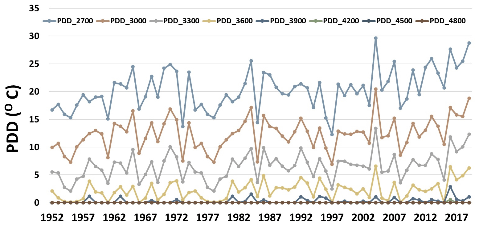
Figure 11 The variation of annual PDD values estimated based on monthly mean temperatures at different elevations in the MBM from 1952 to 2019.

5.3 Influence of changing climate on the area loss

Figure 11 shows the trend of PDD increase over the years in the MBM. All elevations, except 4800 m a.s.l., show an increasing trend of PDD values from 1952 to 2019. Specifically, for the year 1952, since we have only 1 year for the longer-term analysis, it is interesting to look in detail at the climatic conditions prevailing in the region around this period. Looking at the GSB records, the average temperature in the region during the past 10 years before 1952 was −0.987 ^∘C, with average summer temperatures (July, August and September) being 6.783 ^∘C. Year 1947 was particularly hot, with the annual average temperature recorded at −0.275 ^∘C and average summer temperatures at 8.266 ^∘C. The next 30 years after 1952 were more favourable, with average annual temperatures at −1.523 ^∘C and average summer temperatures at 5.256 ^∘C (GSB data provided in the Supplement as “supplementary material 1”). Since 1952 was coming at the back of considerably warmer years, a significant reduction in the surface area of IAs can be expected during this period. Looking at the weather records, the conditions after 1952 for the next 30 years were more favourable.

Figure 12 Variation of the average accumulation rates on steep slopes at different elevations for each period of observation.

Figure 13 Accumulation (steep slopes) trends for the year 2019 at different elevations.

Similarly, Fig. 12 shows the variations in the accumulation rates (average annual accumulation per period) for all elevation bands. The results show only that part of the snowfall which is expected to accumulate on the steep slopes. Except for the highest elevation band, i.e. 4800 m a.s.l., accumulation rates at all elevation bands show a general decreasing trend. For example, at the 3900 m a.s.l. elevation band, accumulation rates fell from 32 mm yr⁻¹ from 1952 to 2001 to 28 mm yr⁻¹ from 2001 to 2012 and further to 18 mm yr⁻¹ between 2012 and 2019. This shows that temperatures in the MBM are increasing, while, on the other hand, accumulation on steep slopes is decreasing over time. Figure 13 shows the annual variation of the accumulation on steep slopes at different elevations. The first observation from this trend shows that very little precipitation accumulates on steep slopes in the winter months, while accumulation occurs almost entirely in the summer months. Further, the accumulation is more significant at higher elevations (4200–4500 m a.s.l.) in the summer months than at lower elevations. At lower elevations, accumulation is predominantly observed in pre-summer (May) and post-summer (October) months.

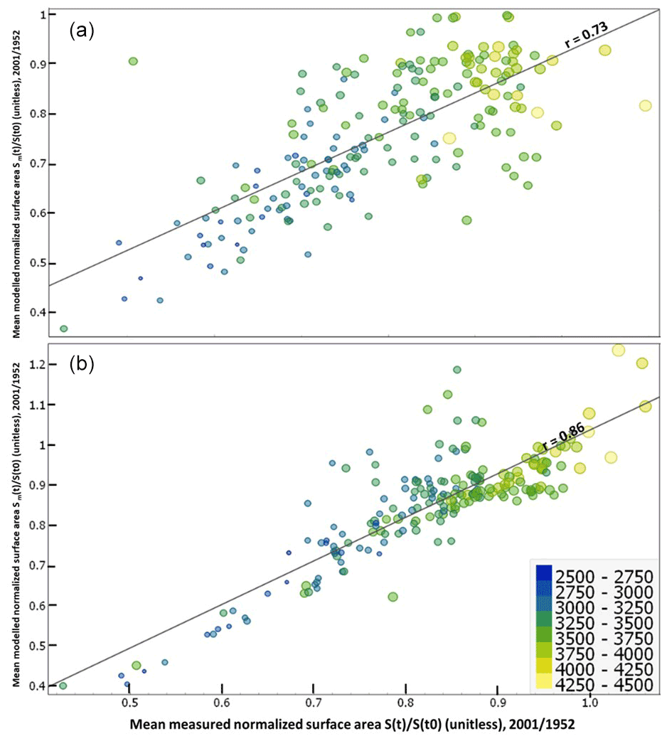
Figure 14 Correlation between the mean normalized measured and modelled surface areas (a) with GSB data transformed to AdM data and (b) with SAFRAN reanalysis data at time t. The colour and size of the ticks represent the mean elevation of the IA.

Figure 14a presents the correlation between the ratio of the mean measured surface area at time t, S(t), to the initial area, S(t₀), with the ratio of the mean modelled surface area using the GSB transformed data to the initial area for 2001 and 1952. We consider the ratio of $S\left(t\right)/S\left(t_{\mathrm{0}}\right)$ as an indicator to estimate the area loss between the two time periods. A high ratio value (i.e. value close to 1) in the present context indicates that the relative surface area loss of IAs between the two periods is comparatively less than that of IAs whose ratio is closer to 0. A value larger than 1 indicates an increase in the surface area over time.

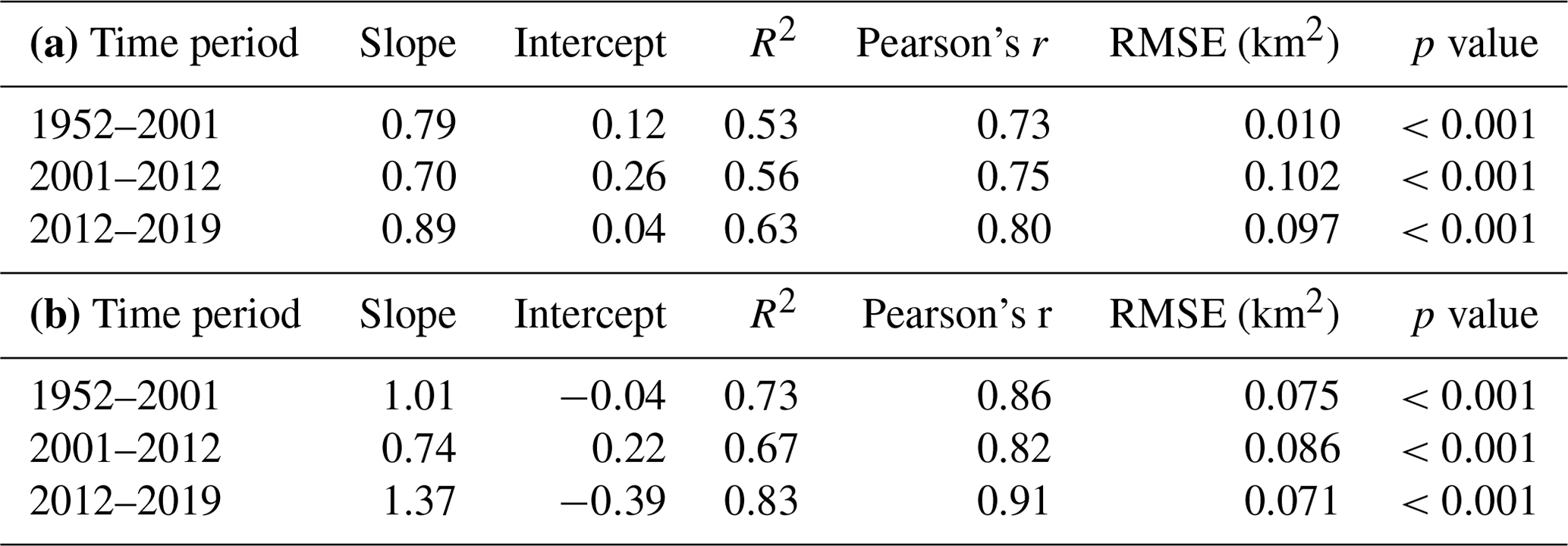
From the results, we do not see a strong correlation (r=0.73) between the modelled area (from GSB transformed climate data) and the measured area for the 200 IAs spread across the MBM (Fig. 14a). However, the correlation improves significantly (r=0.86) when we use the SAFRAN data based on different elevations and remodel the surface area for each IA (Fig. 14b). This can be seen from the values of R², Pearson's r, RMSE and the p value estimates from the T test achieved from both datasets (Table 2). The best-fitting line presents a slope of 1.0 and an intercept of 0.0.

Table 2 Linear regression parameters and correlation metrics for each period (a) using GSB transformed data and (b) using the SAFRAN reanalysis product.

Both figures show that IAs at lower elevations (blue to green colour and small tick size) generally show lower ratio values than IAs at higher elevations (yellowish colours and bigger tick size). This implies that the elevation of the IAs potentially plays a crucial role in their response to the changing climate. Overall, the surface area of IAs decreased throughout the massif from 1952 to 2001 except for four IAs, which showed an increase in surface area. These four IAs are two IAs on the N and NW face of Rochers Rouges Inferieurs (∼4350 and 4050 m a.s.l.) near the Grand Plateau, one IA on the NE face of Col de la Brenva (∼4160 m a.s.l.), and one IA on the S face of Col du Bionnassay (∼4050 m a.s.l.). As observed, all these IAs are located at elevations higher than 4000 m a.s.l. As an exception, it can be expected that a few IAs could show an increase in the surface area. However, this increase is not dramatic (∼10 % increase). The results, however, reaffirm the proficiency of the proposed surface area model in predicting new IA states from the accumulation and ablation proxies. Similar results were observed for the other two time periods, i.e. 2001–2012 and 2012–2019, as seen in Table 2.

5.4 Influence of the local topography and other factors on the area loss of IAs

Each parameter, as described in Sect. 4.2, was individually regressed with the relative area loss of IAs for the three periods, and their influence was assessed by the coefficient of determination (R²) and Pearson's r value.

Table 3 Linear regression parameters and correlation metrics for each studied parameter.

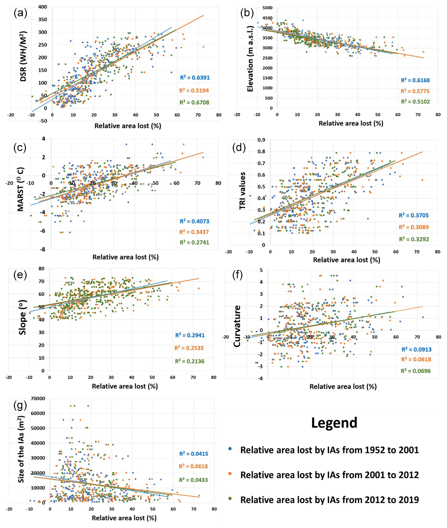
Figure 15 Scatter plots showing relationships between topographic factors and the area loss of IAs from 1952 to 2019. (a) Direct solar radiation, (b) elevation, (c) MARST, (d) TRI, (e) slope, (f) curvature and (g) size of the IAs.

A joint analysis of the surface area lost by the IAs and the direct solar radiation reveals a strong correlation between the values of DSR and the relative surface area loss of IAs for all the three time periods (1952–2001, 2001–2012 and 2012–2019) (Fig. 15a; Table 3). However, this is the first evidence of the potential negative impact of solar radiation on small ice bodies like IAs. Previous analysis of Guillet and Ravanel, 2020, with the climate variables indicated a potential relationship between the elevation and the surface area loss of IAs. This is somewhat statistically significant from the regression analysis, as we found a negative correlation between the surface area loss and the mean elevation of the IAs (Fig. 15b; Table 3). A further comparison of the IAs (200 IAs) distribution with elevation and aspect shows that most IAs (∼77 % of the total number) exist at elevations above 3200 m a.s.l. Further, most IAs (∼56.5 %) exist in the northern aspects (N, NW, NE), while the E and W aspects are the least favoured (Supplement; supplementary material 2). In addition, we found a moderate positive correlation between the average MARST values and the surface area loss of IAs. The correlation observed was not very significant compared to the previous two factors. It indicates that the effect of rock surface temperatures on the area loss of IAs is not strong on a regional scale (Fig. 15c; Table 3). However, this relationship needs to be examined in a more site-specific and localized area to understand better its impact on the surface area loss of IAs. We also observed that the correlation was higher for a more extensive observation period (1952–2001) than for shorter periods. This could suggest that the influence of rock surface temperatures potentially becomes more prominent with a more extensive observation period.

A similar analysis of IA area loss with the TRI showed a weak positive correlation (Fig. 15d; Table 3). An increase in TRI values (i.e. increase in terrain ruggedness) may result in more ice area loss on a site-specific scale, but this relationship is hard to observe globally. Like the results from the analysis with MARST, the strongest correlation was again observed for the largest study period. Further, like the TRI, we also found a weak correlation between the terrain slope and curvature with the surface area loss of IAs. We must note that our criteria for selecting IAs already limit us to areas with slope angles steeper than 40^∘ (Fig. 15e; Table 3). Hence it was difficult to observe any significant impact of terrain slope on the rate of area loss of IAs. Similarly, terrain curvature seems to have the most negligible impact (Fig. 15f; Table 3). As cited in Sect. 4.2. previous studies may have shown that terrain curvatures could play an essential role in the erosion and accumulation dynamics on steep slopes, but this is not the case for IAs in the MBM. We performed the last comparison between the relative surface area loss of IAs with their initial area. Our results were similar to the one Lopez et al. (2010) reported, as we did not find any correlation between the two quantities (Fig. 15g; Table 3).

6 Discussion

6.1 Area loss of ice aprons and the role of the changing climate

As observed from the results in Sect. 5.2, IAs have been losing surface area at an alarming rate. This rate of surface area loss is disconcerting because, compared to the glaciers in the MBM, the IAs are losing their area at a higher rate (∼24 % for glaciers from the end of LIA until 2008, according to Gardent et al., 2014, while IAs have lost ∼47 % of surface area in the last 70 years). The small size of IAs makes them more vulnerable to global warming than large glaciers. An increase in average annual temperatures and a decrease in precipitation rates put the existing IAs at risk of losing their mass entirely before the end of this century. In addition, considering that the effects of local topography are also more pronounced in the case of IAs than for large glaciers, continuous monitoring of these critical ice bodies has become imperative. Results discussed in Sect. 5.3 indicated the strong influence of temperature and precipitation on the surface area changes of IAs. The results raise further questions regarding the sensitivity of the IAs to extreme weather events, like the heatwaves experienced in the study region. Unfortunately, our sampling rate does not allow us to quantify the effects of individual extreme weather events. Nevertheless, there is a strong argument in favour that these events, especially in the past two decades, cause the IAs to lose mass more rapidly than in the previous decades. Further, the heatwaves occurring during winter and midsummer, when the IA surfaces are free of snow, will have the worst adverse effect.

As suggested by Meehl and Tebaldi (2004), with an increase in the intensity and frequency of extreme events in the coming decades, understanding the effects of climate variables on the sensitivity of IAs is even more critical.

Further, several authors have previously also accounted for the variations in solar radiation in mass balance modelling studies (Huss et al., 2009; Thibert et al., 2018). Our results showed a strong correlation of DSR with area change, making this argument stronger. However, since the focus was to show the impact of climate variables separately, we preferred a temperature-index model as the first approach. However, we expect solar radiation to play a significant role in the sensitivity of ice aprons, and future studies on ice apron evolutions in the 21st century should address this question.

6.2 Area loss of ice aprons and the role of topographic parameters

Since ice/glacier bodies within the same climate regime can also respond to climate change differently, the last part of the analysis (Sect. 5.4) was dedicated to understanding the linkages of local topographic factors to the surface area loss of IAs. As reported previously by Salerno et al. (2017), some local topographic factors influence the response of IAs to climate change more significantly than others. A first analysis showed that IAs that receive more solar radiation from the sun throughout the year lose their surface area faster than those that receive less DSR. Similar results for other regions in mountain environments have also been reported previously by Oerlemans and Klok (2002), Mölg (2004), and Johnson and Rupper (2020). Incoming solar radiation is an essential component of all surface energy and mass balance models. But the significance of DSR on the surface area loss of small ice bodies like IAs is reported for the first time in our study.

Further, the correlation between elevation and surface area loss of IAs was the second most significant of all topographic factors. IAs located at lower elevations are potentially subject to more intense degradation and lose their surface area faster than those at higher elevations. On a more local scale, other topographic factors could also play a critical role in the surface area variations of IAs. However, elevation seems to be a dominant causative factor on a regional scale. Elevation strongly influences meteorological conditions (temperature, precipitation and wind speeds) and permafrost; this likely strongly influences the durability of IAs in the context of changing climate. Hantel et al. (2012) suggested the median summer snowline for the Alps to be at 3083±121 m a.s.l. (1961–2010), while Rabatel et al. (2013) documented the regional ELA at 3035±120 m a.s.l. (1984–2010). Rabatel et al. (2013) further described the rising of the ELA to 3250±135 m a.s.l. during the 2003 heatwave. Subsequent heatwaves of 2006, 2015 and 2019 would have likely resulted in similar scenarios (Hoy et al., 2017). Since ∼77 % of the total IAs reported in this study exist at elevations above 3200 m a.s.l., the rising of the ELA in future climate scenarios risks more IAs towards faster degradation and disappearance. An example of this is the case of the IA on the north face of Aiguille des Grands Charmoz (3445 m a.s.l.), which completely disappeared during the 2017 summer heatwave (Guillet and Ravanel, 2020).

In addition, on a local scale, some correlation between the rock surface temperatures and the area loss of IAs was observed from the analysis. Guillet et al. (2021) suggested that IAs are cold ice bodies that exist predominantly on permafrost-affected rock walls. They further reported temperatures <0 ^∘C at the base of the ice core taken from the IA on the north face of Triangle du Tacul (3970 m a.s.l.). Heating from rock surfaces is predominantly the cause of permafrost degradation, which further affects mountain slope stability, leading to an increased rock mass wasting (Magnin et al., 2017). Cold surfaces demonstrate more ice cohesion with the underlying surfaces, while a rise in surface temperatures decreases basal cohesion, increasing the sliding process and leading to more ice flow (Deline et al., 2015). Thus, it is likely that underlying permafrost conditions aid the sustainability of IAs in the long term, and an increase in rock surface temperatures around IAs could result in IAs losing mass more rapidly.

Kaushik et al. (2021) further showed that most IAs exist in extremely rugged terrains: 51 % of the total IAs mapped exist in the TRI's high and very high ruggedness class, while only 8 % exist in the low ruggedness. Thus, comparing the terrain ruggedness to the area loss of IAs makes sense since the topography around the snow/ice bodies can critically influence their stability (Deline et al., 2015). Increasing terrain ruggedness is associated with slope instability and further ice volume loss. However, for our study, this relation was not very pronounced, showing that the topography's ruggedness does not substantially affect the area loss of IAs.

Previous analysis by Kaushik et al. (2021) also showed that most IAs in the MBM (83 %) lie at mean slopes between 40 and 65^∘. Increasing slope steepness limits accumulation, while avalanches further scour away snow from the surface of the IA, thus exposing the ice directly to the sun and wind (Vionnet et al., 2012). However, the differences in slope angles of the IAs were not a dominant factor affecting the rates of area loss. A plausible explanation for this could be that since we limit the slope criteria to >40^∘ and most IAs lie in the range of 40 to 65^∘ slope, the effect of terrain slope is not as well pronounced as it would be between low (<15^∘) and extreme slopes (>65^∘). Similar results were observed by Li et al. (2011), as they observed very slight variations in area loss for small glaciers with differences in slope. They suggested other local topographic factors could mitigate the effects of slope in the event of small ice/snow bodies.

Similarly, terrain curvature also has a negligible effect on the surface area loss of IAs. As suggested by Alkhasawneh et al. (2013) and Yanuarsyah and Khairiah (2017), convex profile curvature favours the erosion processes, while in locations with concave curvature, the deposition process can be predominant. Over time, the terrain curvature can be a dominant factor in the dynamics of glacier/ice bodies, but this relation was not established for our study.

At last, a comparison of the rate of surface area loss of IAs with the original size of the IAs was performed, and we observed no correlation between the two factors. Although previous studies by Paul et al. (2004), Jiskoot et al. (2009) and Garg et al. (2017) have shown the correlation between the size of the ice/glacier bodies with the area loss, this is not evident in our case. Unlike previous studies, which considered different glaciers ranging in size from less than a square kilometre (km²) to several hundred square kilometres, IAs are small ice bodies (0.0005 to 0.1 km²). Hence, it is plausible that the effect of IA size on area loss rate is not pronounced in our case. Similar results were shown by Lopez et al. (2010), who analysed 72 glaciers in South America and reported no correlation between the glacier length and the area loss of glaciers.

Another critical factor to consider, along with the impact of topography, is the role of avalanches in the erosion and deposition processes on the IA surface. Analysis of the ice core from the N face of Triangle du Tacul showed that IAs are almost immobile cold ice bodies (Guillet et al., 2021). Hence IAs do not directly participate in feeding the larger glacier systems below them. However, the avalanches triggered above can bring fresh snow/debris and lead to erosion or deposition on the IA surface. We expect this factor to also play a role in the area change dynamics of the IA, which we have not considered as part of this study. Although this impact on the scale of an IA is tough to determine, future studies should focus on ascertaining this impact at least on a local site-specific scale.

7 Conclusions

This study makes the first attempt to understand the dynamics of IAs concerning the changing climate and topographic factors at a regional scale. IAs are very small ice features but highly critical components of the mountain cryosphere. Because of the difficulties associated with their monitoring and relative unimportance to mountain hydrology, no studies solely based on their evolution on a regional scale have been performed before. This paper presented an analysis of 200 IAs spread throughout the MBM and existing in different topographic settings to understand their dynamics in the context of climate warming. For this purpose, we accurately mapped the IAs on very high-resolution aerial and satellite images available for 1952, 2001, 2012 and 2019. Using our extensive database of IAs, we compared the total area variation of IAs for three periods. Further, we also attempted to establish a relationship between the surface area lost by IAs with meteorological parameters (i.e. temperature and precipitation) and their associated topographic parameters.

Some important outcomes from the study are the following.

• Over the study period 1952–2019, IAs have lost their surface area at a very alarming rate. The total area of IAs in MBM was 7.93 km² in 1952, dropping to 5.91 km² in 2001, 4.91 km² in 2012, and 4.21 km² in 2019 (∼47 % drop in total surface area in less than three-quarters of a century).

• The observed rate of relative area loss in the last 18 years (∼29 %) is more than the overall area loss during the 48 previous years (1952–2001; ∼26 %).

• Results from the analysis of IA surface area loss and meteorological parameters (i.e. temperature and precipitation) conclusively proved the strong impact of these parameters on the behaviour of small ice bodies like IAs.

• Further analysis of IA surface area loss with different topographic parameters showed a strong correlation of IA surface area loss with the DSR and elevation. Other factors like MARST, TRI and mean terrain slope could also play an important role locally, but their effect is not significant regionally. Terrain curvature and the size of the IAs were not found to impact the IA surface area loss significantly.

Looking at the melting rate of IAs and the future predictions of global climate change, it is evident that these small and critical ice bodies are most vulnerable to adverse impacts. It is hard to imagine any of the IAs surviving the next few decades with increasing temperatures at the present and future melting rates. The loss of IAs will thus be the loss of crucial glacial heritages and playgrounds for the iconic practice of mountaineering. Hopefully, this study forms a basis to encourage further studies on IAs.