Evaluating simplifications of subsurface process representations for field-scale permafrost hydrology models

Permafrost degradation within a warming climate poses a significant environmental threat through both the permafrost carbon feedback and damage to human communities and infrastructure. Understanding this threat relies on better understanding and numerical representation of thermo-hydrological permafrost processes and the subsequent accurate prediction of permafrost dynamics. All models include simplified assumptions, implying a tradeoff between model complexity and prediction accuracy. The main purpose of this work is to investigate this tradeoff when applying the following commonly made assumptions: (1) assuming equal density of ice and liquid water in frozen soil, (2) neglecting the effect of cryosuction in unsaturated freezing soil, and (3) neglecting advective heat transport during soil freezing and thaw. This study designed a set of 62 numerical experiments using the Advanced Terrestrial Simulator (ATS v1.2) to evaluate the effects of these choices on permafrost hydrological outputs, including both integrated and pointwise quantities. Simulations were conducted under different climate conditions and soil properties from three different sites in both column- and hillslope-scale configurations. Results showed that amongst the three physical assumptions, soil cryosuction is the most crucial yet commonly ignored process. Neglecting cryosuction, on average, can cause 10 %–20 % error in predicting evaporation, 50 %–60 % error in discharge, 10 %–30 % error in thaw depth, and 10 %–30 % error in soil temperature at 1 m beneath the surface. The prediction error for subsurface temperature and water saturation is more obvious at hillslope scales due to the presence of lateral flux. By comparison, using equal ice–liquid density has a minor impact on most hydrological metrics of interest but significantly affects soil water saturation with an averaged 5 %–15 % error. Neglecting advective heat transport presents the least error, 5 % or even much lower, in most metrics of interest for a large-scale Arctic tundra system without apparent influence caused by localized groundwater flow, and it can decrease the simulation time at hillslope scales by 40 %–80 %. By challenging these commonly made assumptions, this work provides permafrost hydrology scientists an important context for understanding the underlying physical processes, including allowing modelers to better choose the appropriate process representation for a given modeling experiment.

1 Introduction

Permafrost describes a state of ground which stays frozen continuously over multiple years, which may cover an entire region (e.g., Arctic tundra) or occur in isolation (e.g., alpine top). From the perspective of scope, permafrost occupies approximately 23.9 % (22.79 ×10⁶ km²) of the exposed land area of the Northern Hemisphere (Zhang et al., 2008), as well as alpine regions and Antarctica in the Southern Hemisphere. Permafrost areas store a vast amount of organic carbon, of which most is stored in perennially frozen soils (Hugelius et al., 2014). If the organic carbon is exposed due to permafrost thaw, it is likely to decay with microbial activity, releasing greenhouse gas to the atmosphere and exacerbating global warming. In Arctic tundra, permafrost also plays an important role in maintaining water, habitat of wildlife, landscape, and infrastructure (Berteaux et al., 2017; Dearborn et al., 2021; Hjort et al., 2018; Sugimoto et al., 2002). Permafrost degradation may cause significant damage to the local ecosystem, reshape the surface and subsurface hydrology, and eventually influence the global biosphere (Cheng and Wu, 2007; Jorgenson et al., 2001; Tesi et al., 2016; Walvoord and Kurylyk, 2016). Therefore, the occurrent and potential impacts motivate the development of computational models with the goal of better understanding the thermal and hydrological processes in permafrost regions and consequently to predict permafrost thaw more accurately.

Simulating soil freezing and thaw processes is a challenging task that incorporates mass and energy transfer among atmosphere, snowpack, land surface (perhaps with free water), and a variably saturated subsurface. Several hydrological models with different complexity and applicable scales have been developed to investigate the complicated interactions. Reviews of permafrost models based on empirical and physical representations using analytical and numerical solutions can be found in Bui et al. (2020), Dall'Amico et al. (2011), Grenier et al. (2018), Jan et al. (2020), Kurylyk et al. (2014), Kurylyk and Watanabe (20130), and Riseborough et al. (2008). Process-rich models which aim to predict permafrost change through direct simulation of mass and energy transport, such as the Advanced Terrestrial Simulator (ATS; Painter et al., 2016), GEOtop (Endrizzi et al., 2014), CryoGrid 3 (Westermann et al., 2016), PFLOTRAN-ICE (Karra et al., 2014), and SUTRA-ICE (McKenzie et al., 2007), have been demonstrated to describe thermal permafrost hydrology under various climate conditions. Nominally, representing more physical process complexity should improve predictions of permafrost change, but the degree to which each process affects metrics of permafrost hydrology is highly uncertain and likely differs by scale. Philosophically, models provide a useful tool precisely because they allow counterfactual experiments in which processes are simplified to understand the relative importance of those processes; thus, challenging assumptions about process simplifications are a significant part of both general process understanding, benefiting the permafrost hydrology community writ large, and model representations, benefiting the community of model developers and users.

Even in the most process-rich models of permafrost change, three such physical simplifications are often made: representing water at constant density (thereby neglecting the expansion of ice relative to liquid water), neglecting cryosuction of water in unsaturated, partially frozen soils, and neglecting advective heat transport.

First, because of the lower density of ice than liquid water, freezing water must expand the volume of the porous media, push liquid water into nearby volume, or otherwise expand the volume occupied by that water. As most of the current set of models operate under the assumption of a rigid solid matrix and thus the absence of mechanical equations describing matrix deformation or frost heave, including this expansion typically results in large pressures that must be offset by grain compressibility or another mechanism. Therefore, the densities of ice and liquid water are frequently assumed equal (e.g., Dall'Amico et al., 2011; Devoie and Craig, 2020; Weismüller et al., 2011). It is uncertain whether this simplification affects predictions of permafrost change and thermal hydrology.

Second, cryosuction describes the redistribution of water in partially frozen, unsaturated soils caused by increased matric suction. At the interface of ice and liquid water, negative pressures result in the migration of liquid water toward the freezing front and the subsequent increase in ice content. Several approaches representing cryosuction in models are used (Dall'Amico et al., 2011; Noh et al., 2012; Painter and Karra, 2014; Stuurop et al., 2021), either in an empirical form or physically derived from the generalized Clapeyron equation. Other process-rich models have ignored cryosuction entirely (McKenzie et al., 2007; Viterbo et al., 1999). Dall'Amico et al. (2011), Painter (2011), and Painter and Karra (2014) evaluated their respective Clapeyron-equation-based cryosuction models in soil column freezing simulations and presented a good match between simulations and laboratory experiments in total water content (liquid and ice). Recently, Stuurop et al. (2021) applied an empirical expression, a physics-based expression, and no cryosuction in simulating the soil column freezing process. They compared the simulated results with observations from laboratory experiments. This comparison demonstrated minor differences between empirical and Clapeyron-based cryosuction expressions, but the simulation without cryosuction cannot predict the distribution of total water content in a laboratory-scale soil column. To our knowledge, there is still no literature showing the effect of cryosuction on plot-scale permafrost predictions.

Third, heat transport in process-rich models is described using an energy conservation equation, mainly including heat conduction, latent heat exchange, and heat advection. From a continuum-scale perspective, conductive heat transport is expressed in the form of a diffusive term based on Fourier's law. Latent heat exchange accompanies phase change, which alters the system enthalpy. Advective heat transport describes the energy exchange caused by the flow of liquid water driven by a hydraulic gradient (i.e., forced convection), which is expressed through an advective term in energy balance equations. Additionally, other mechanisms that control heat transport, such as water vapor movement, thermal dispersion, etc., are neglected by nearly all models of permafrost and are not considered here. Several studies have demonstrated the importance of advective heat transport in permafrost hydrology through field observation analysis or modeling comparison. Such situations in which advective heat transport makes important contributions roughly fall into three categories. The first centers on the development of taliks beneath lakes, ponds, topographic depressions, or other discontinuous permafrost effects (e.g., Dagenais et al., 2020; Liu et al., 2022; Luethi et al., 2017; McKenzie and Voss, 2013; Rowland et al., 2011). The second focuses on microtopographic features that focus a significant amount of water through small areas. This includes both low-center ice wedge polygons associated with the formation of thermokarst ponds (e.g., Abolt et al., 2020; Harp et al., 2021) and thermo-erosion gullies (e.g., Fortier et al., 2007; Godin et al., 2014). In these cases, large, focused flows across small spatial scales allow advective heat transport to dominate. The last category includes those studying the construction and maintenance of infrastructure influenced by groundwater flow (e.g., Chen et al., 2020). Thus, these studies focus on either location-specific or scale-limited problems. As McKenzie and Voss (2013) stated, whether heat advection outweighs heat conduction depends on soil permeability, topography, and groundwater availability. Relative to these special cases at small scales, we are more interested in the extent to which advective heat transport associated with liquid water flow contributes to permafrost hydrologic change in a hillslope-scale or larger Arctic system. The Arctic systems, discussed hereinafter in this paper, refer to those with negligible influence caused by localized groundwater flow features as the three categories mentioned above.

To clarify the significant differences in model representations of permafrost, we investigate the influence of including or not including these processes on permafrost change at plot-to-hillslope scales. For ice density, we compare simulations with and without differences in ice density relative to water density; for cryosuction, we compare simulations using a Clapeyron-equation-based expression and excluding the cryosuction effect; and for heat transport, we compare simulations including or neglecting advective heat transport. All comparisons are carried out across a range of Arctic climate conditions and soil properties from three different sites. Both 1D soil-column-scale and 2D hillslope-scale models are considered, in which varying hillslope geometries (i.e., convergent/divergent hillslope) and aspects (i.e., north/south) are included. The aim of this study is to provide better understanding of physical processes to permafrost hydrologists in general, as well as to offer some concrete insights to the model users and developers working on the process-rich models with similar theories and equation basis.

2 Theory

The Advanced Terrestrial Simulator (ATS v1.2) (Coon et al., 2020) configured in permafrost mode (Jan et al., 2018, 2020; Painter et al., 2016) was used to implement all numerical experiments in this study. ATS is a process-rich code developed for simulating integrated surface and subsurface hydrological processes, specifically capable of permafrost applications. It has been shown to successfully compare to observations of seasonal soil freezing and thaw processes at different scales. This includes 1D models of vertical energy transport typical of large-scale flatter regions (Atchley et al., 2015) and 2D models admitting lateral flow and transport in Arctic fens (Sjöberg et al., 2016) and polygonal ground (Jan et al., 2020). The permafrost configuration of ATS comprises coupled water flow and energy transfer within variably saturated soils and at land surfaces, a surface energy balance model describing thermal processes in snow, and a snow distribution module for surface microtopography (Painter et al., 2016). The subsurface system solves a three-phase (liquid, ice, gas), two-component (water vapor, air) Richards-type mass balance equation with Darcy's law and an advection–conduction energy balance equation. The surface system includes an overland flow model with diffusion wave approximation and an energy balance equation with an introduced temperature-dependent factor describing the effect of surface water freezing. The subsurface system and surface system are coupled through the continuity of pressure, temperature, and the corresponding fluxes by incorporating the surface equations as boundary conditions of the subsurface equations (Coon et al., 2020). The evolution of a snowpack and its effect on the surface energy balance is described using an energy balance approach based on a subgrid model concept that includes all major heat fluxes at the land surface. For a more detailed description of the permafrost configuration and implementation in ATS, as well as key mathematical equations, the reader is referred to Painter et al. (2016). Changes in this “most complex” model of permafrost hydrology are enabled by the Arcos multiphysics library leveraged in ATS; this allows the precise model physics to be specified and configured at runtime through the use of a dependency graph describing swappable components in the model physics (Coon et al., 2016).

2.1 Ice density

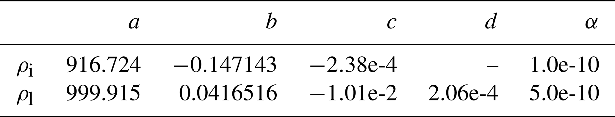
The density of ice (kg m⁻³) is represented as a Taylor series expansion in both temperature and pressure:

$$\begin{array}{}\text{(1)}& {\mathit{\rho }}_{\mathrm{i}}=\left[a+\left(b+c\mathrm{\Delta }T\right)\times \mathrm{\Delta }T\right]\times \left(\mathrm{1}+\mathit{\alpha }\mathrm{\Delta }p\right),\end{array}$$

and the density of liquid water (kg m⁻³) is represented as

$$\begin{array}{}\text{(2)}& {\mathit{\rho }}_{\mathrm{l}}=\left[a+\left(b+\left(c+d\mathrm{\Delta }T\right)\times \mathrm{\Delta }T\right)\times \mathrm{\Delta }T\right]\times \left(\mathrm{1}+\mathit{\alpha }\mathrm{\Delta }p\right),\end{array}$$

where $\mathrm{\Delta }T=T-\mathrm{273.15}$, $\mathrm{\Delta }p=p_{\mathrm{l}}-\mathrm{1}e\mathrm{5}$, T and p_l are temperature (K) and liquid pressure (>101 325 Pa), respectively, and a, b, c, d, and α are constant coefficients, listed in Table 1. Under conditions of equal density, we assume ρ_i=ρ_l.

Table 1 Coefficients in density of ice and liquid.

2.2 Cryosuction

Several models are available in the literature describing the relationship between unfrozen water content and temperature or matric suction (e.g., Ren et al., 2017; Stuurop et al., 2021), which is also termed the soil freezing characteristic curve. These models are either associated with temperature empirically or related to the soil water retention curve through the Clapeyron equation. The latter approach normally incorporates the soil cryosuction process, while the former does not. Painter and Karra (2014) proposed a constitutive model which relates the soil unfrozen water content with the van Genuchten model (van Genuchten, 1980) based on the Clapeyron equation:

$$\begin{array}{}\text{(3)}& \begin{array}{l}{s}_{\mathrm{l}}=\left\{\begin{array}{l}{S}_{\ast }\left(-\mathit{\beta }{\mathit{\rho }}_{\mathrm{l}}{L}_{\mathrm{f}}\mathit{\vartheta }\right)\mathit{\vartheta }<{\mathit{\vartheta }}_{\mathrm{f}},\\ S_{\ast }\left(p_{\mathrm{g}}-p_{\mathrm{l}}\right)\mathit{\vartheta }\ge {\mathit{\vartheta }}_{\mathrm{f}},\end{array}\right.\\ s_{\mathrm{i}}=\mathrm{1}-s_{\mathrm{l}}/S_{\ast }\left(p_{\mathrm{g}}-p_{\mathrm{l}}\right),\\ \mathit{\vartheta }=\frac{T\left(\mathrm{K}\right)-\mathrm{273.15}}{\mathrm{273.15}},{\mathit{\vartheta }}_{\mathrm{f}}=-\frac{{\mathit{\psi }}_{\ast }\left(\mathrm{1}-s_{\mathrm{g}}\right)}{\mathit{\beta }{L}_{\mathrm{f}}{\mathit{\rho }}_{\mathrm{l}}}\end{array}\end{array}$$

where s_n is the saturation of n phase, the subscripts n= l, i, and g are liquid, ice, and gas phases, respectively, β is a coefficient, L_f is the heat fusion of ice, p_n (n= l, g) is the pressure of n phase, and S_∗ is the van Genuchten model. This physically derived formulation can describe the change in matric suction in the frozen zone due to the change in ice content, and it thus has the capacity to represent cryosuction.

Alternatively, the unfrozen water content can be also expressed as a single-variable function dependent on sub-freezing temperature for a given soil, ignoring the effect of cryosuction, such as the following (McKenzie et al., 2007):

$$\begin{array}{}\text{(4)}& \begin{array}{rl}& s_{\mathrm{l}}=s_{\mathrm{r}}+\left(s_{\mathrm{sat}}-s_{\mathrm{r}}\right)\exp \left[-{\left({\displaystyle \frac{T\left(\mathrm{K}\right)-\mathrm{273.15}}{\mathit{\omega }}}\right)}^{\mathrm{2}}\right],\\ & s_{\mathrm{i}}=S_{\ast }\left(p_{\mathrm{g}}-p_{\mathrm{l}}\right)-s_{\mathrm{l}},\end{array}\end{array}$$

where s_r and s_sat are saturations of liquid water at residual and saturated conditions, respectively, and ω is a constant coefficient. In this case, the van Genuchten model was used to determine the total water content, including liquid water and ice.

2.3 Advective heat transport

The energy conservation equation of the subsurface system is given by

$$\begin{array}{}\text{(5)}& \begin{array}{rl}{\displaystyle \frac{\partial }{\partial t}}& \left[\mathit{\varphi }{\sum }_{n=\mathrm{l},\mathrm{i},\mathrm{g}}\left({\mathit{\rho }}_n{s}_n{u}_n\right)+\left(\mathrm{1}-\mathit{\varphi }\right)c_{\mathrm{v},\mathrm{soil}}T\right]\\ & +\underset{\text{advective heat}}{\underbrace{\mathrm{\nabla }\cdot \left({\mathit{\rho }}_{\mathrm{l}}{h}_{\mathrm{l}}{\mathbf{V}}_{\mathrm{l}}\right)}}\underset{\text{conductive heat}}{\underbrace{-\mathrm{\nabla }\cdot \left({\mathit{\kappa }}_{\mathrm{e}}\mathrm{\nabla }T\right)}}=Q_{\mathrm{E}},\end{array}\end{array}$$

where ϕ is porosity, u_n is the specific internal energy of phase ($n\mathit{ϵ}\mathit{\{}\mathrm{l},\mathrm{i},\mathrm{g}\mathit{\}}$), and c_v,soil (J m⁻³ K⁻¹) is the volumetric heat capacity of the soil grains. The second and third terms represent the advective and conductive heat transport in the subsurface, in which h_l (J mol⁻¹) is the specific enthalpy of liquid, V_l (m s⁻¹) is the velocity vector of liquid water determined by Darcy's law, and κ_e (W m⁻¹ K⁻¹) is the effective thermal conductivity of the bulk material including soil, air, liquid water, and ice. Q_E is the sum of all thermal energy sources (W m⁻³).

Similarly, the energy balance equation of the surface system is

$$\begin{array}{}\text{(6)}& \begin{array}{rl}{\displaystyle \frac{\partial }{\partial t}}& \left\{\left[\mathit{\chi }{\mathit{\rho }}_{\mathrm{l}}{u}_{\mathrm{l}}+\left(\mathrm{1}-\mathit{\chi }\right){\mathit{\rho }}_{\mathrm{i}}{u}_{\mathrm{i}}\right]{\mathit{\delta }}_{\mathrm{w}}\right\}\\ & +\underset{\text{advective heat}}{\underbrace{\mathrm{\nabla }\cdot \left(h_{\mathrm{l}}\mathit{\chi }{\mathit{\rho }}_{\mathrm{l}}{\mathit{\delta }}_{\mathrm{w}}{\mathbf{U}}_{\mathrm{w}}\right)}}\underset{\text{conductive heat}}{\underbrace{-\mathrm{\nabla }\cdot \mathit{\left\{}\right[\mathit{\chi }{\mathit{\kappa }}_{\mathrm{l}}+(\mathrm{1}-\mathit{\chi }){\mathit{\kappa }}_{\mathrm{i}}\left]{\mathit{\delta }}_{\mathrm{w}}\mathrm{\nabla }T\mathit{\right\}}}}\\ & =Q_{\mathrm{net}},\end{array}\end{array}$$

in which χ is the unfrozen fraction of surface determined by surface temperature, δ_w is ponded depth (m), and U_w (m s⁻¹) is the velocity vector of liquid water on the surface determined by the diffusion wave approximated St. Venant equations (Gottardi and Venutelli, 1993) and Manning equation (Wasantha Lal, 1998), κ_n (W m⁻¹ K⁻¹) is the thermal conductivity of n phase (n= l, i), and Q_net (W m⁻³) is the net thermal energy into and out of the ground surface, including that from solar radiation, rain and snowmelt, water loss by evaporation and to the subsurface, and conductive and advected heat transport to/from the subsurface. The second and third terms represent the (lateral) advective and conductive heat transport that occur across the land surface.

3 Methods

To evaluate the impact of representation of ice density, cryosuction, and advective heat transport in permafrost modeling under different climate conditions and soil properties, we selected three sites for their variance in climactic condition: Utqiagvik (Barrow Environmental Observatory; 71.3225^∘ N, 156.6231^∘ W), the headwaters of the Sagavanirktok (Sag) River (68.251^∘ N, 149.092^∘ W), and the Teller Road Mile Marker 27 site on the Seward Peninsula (64.73^∘ N, 165.95^∘ W) in Alaska. The simulated hydrological outputs for each site are compared in both column and hillslope scenarios. Column scenarios represent expansive flat regions typical of the Arctic coastal plains dominated by vertical infiltration and heat transport, and hillslope scenarios are representative of the headwater, hilly terrain typical of the more inland permafrost.

In hillslope scenarios, hillslopes with northern and southern aspects are considered to investigate physics representation comparisons under the same climate and soil condition (i.e., at a given site) but different solar radiation incidence. Furthermore, hillslopes with both convergent and divergent geometries are included to compare the sensitivity of simulated discharge on process representation. These scenarios can incorporate many types of Arctic systems at the described plot-to-regional scales but explicitly ignore the effects of microtopography or other local-scale focusing mechanisms such as water tracts or thermo-erosion gullies. The objective is to reach a conclusion on the influence of the three physics representations that can be widely applicable in many Arctic systems.

3.1 Field data description

For each site, data used in each simulation comprise meteorological forcing datasets for the period 2011–2020, averaged wind speed, and soil properties.

Meteorological forcing datasets are taken from the Daymet version 4 dataset (Thornton et al., 2020), which provides observation-based, daily averaged weather variables through statistical modeling techniques at 1 km spatial resolution (Thornton et al., 2021). Variables that are used in simulations include daily average air temperature (calculated as the mean of Daymet's daily minimum and maximum values), relative humidity (calculated from air temperature and Daymet's vapor pressure), incoming shortwave radiation (W m⁻²) (calculated as a product of Daymet's daylit incoming radiation and daylength), and total precipitation (m s⁻¹), which is split into snow and rain based upon the air temperature. Figure 1 illustrates the precipitation of rain, snow, and air temperature at the three sites from 2011 to 2020, where the points represent the corresponding averaged values per year. In terms of the forcing conditions, the annual rainfall of the Sag and Teller sites ranges between 20 and 40 mm d⁻¹ over the 10 years, more than twice the rainfall typical of the Barrow site. In addition, Sag has a significantly larger amount of snow every year that is over double that at the Teller site and almost 5 times larger compared to the Barrow site. For the air temperature, Sag and Barrow are similar and colder than Teller by 7–8^∘C. In general, the Barrow site is dry and cold, the Sag site is wet and cold, and the Teller site is wet and warm.

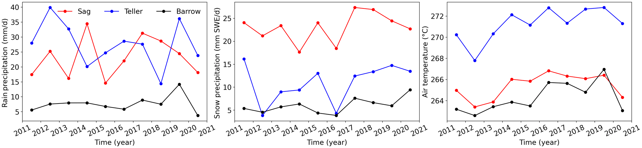
Figure 1 Precipitation and air temperature of sites Barrow, Sag, and Teller from year 2011 to 2020.

In addition to the time series of forcing data from Daymet, we used an average wind speed for each site. For Barrow and Teller, the average wind speed was estimated from the measurement taken by the Next-Generation Ecosystem Experiments (NGEE) Arctic project. At Barrow, the measurement was taken at area A (71.2815^∘ N, 156.6108 ^∘ W) at the height of 1.3 m above the surface (Hinzman et al., 2014). At Teller, the measurement at 3.8 m above the surface of a lower level of the watershed (Busey et al., 2017) was used. For Sag, the average wind speed was estimated based on the measurement at the Toolik Lake field site (near to Sag River) at the height of 3.1 m above the surface, which is accessible through the National Ecological Observatory Network (NEON, 2021).

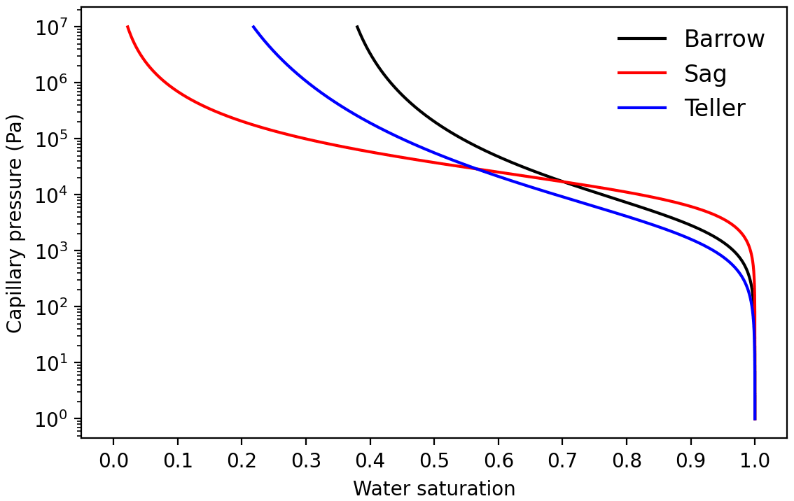
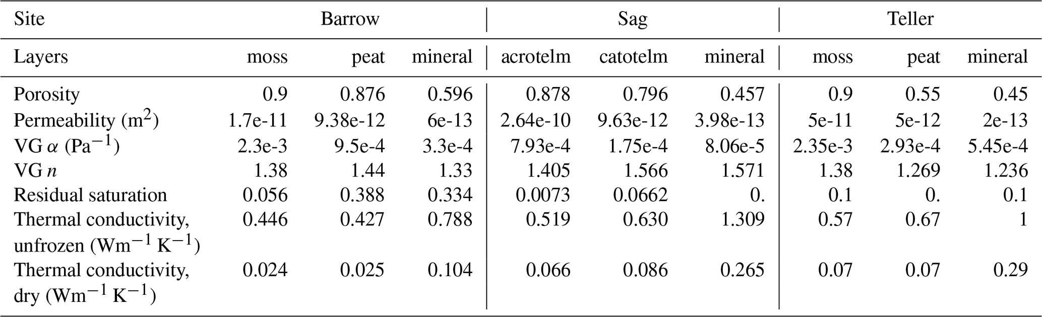
The soil properties of Barrow, Sag, and Teller, including porosity, permeability, van Genuchten parameters, and thermal conductivity parameters, were chosen from previous modeling studies at these sites (Atchley et al., 2015; Jafarov et al., 2018; O'Connor et al., 2020; see Table 2). Roughly, the soil profile of each site is composed of two materials: the top organic-rich layer, comprising mosses, peats, and other organic rich soils measuring approximately 10–30 cm in thickness, and the principal mineral soil. There is minor difference in thermal conductivity parameters among the three sites, and soil permeability is also at the same order of magnitude. The soil-water characteristic curve (SWCC) of the principal mineral soil of Barrow, Sag, and Teller, shown in Fig. 2, indicates that the soil properties at Barrow and Teller are relatively similar, while Sag differs from the other two with a relatively flat SWCC.

Figure 2 Soil-water characteristic curve (SWCC) of soil in Barrow, Sag, and Teller.

Usually, at the hillslope scale, the thickness of organic layers of a watershed varies from the toe-slope, through a steeper mid-hill, and up to the flat top. Typically, thicker organic layers may exist at the top and bottom compared to the mid-hillslope. The low thermal conductivity of organic layers can impede the heat transport between the air and the underlying mineral soil, resulting in varying thaw depth (or permafrost table depth) along a hillslope, which has been observed at Teller (Jafarov et al., 2018). In this paper, hillslope meshes were constructed following this observation so that the organic layers are thicker at the top and bottom of a hillslope, as described in the next section.

3.2 Mesh design and material properties

The comparison of different physics representations was conducted in both column and hillslope scenarios.

The column model was designed as a 1D, 50 m deep domain. The column domain was discretized into 78 cells with gradually increasing cell thickness, starting from 2 cm at the soil surface to 2 m at the bottom of the domain. We assigned different material properties to the cells to represent different soil layers. A column domain is divided into three layers, and the thickness of each layer was designed differently among the three sites according to geological observations (Jan et al., 2020; O'Connor et al., 2020; NGEE-Arctic). Specifically, from top to bottom, the three layers of the Barrow soil column are 2 cm thick moss, 8 cm thick peat, and mineral; for Teller, the soil column consists of a 4 cm moss layer, a 22 cm peat layer, and mineral; and the three layers of the Sag soil column are acrotelm, catotelm, with thicknesses of 10 and 14 cm, respectively, and the remainder mineral. The soil properties of each layer at the three sites are listed in Table 2.

Table 2 Soil properties of three soil layers of all sites used in this paper.

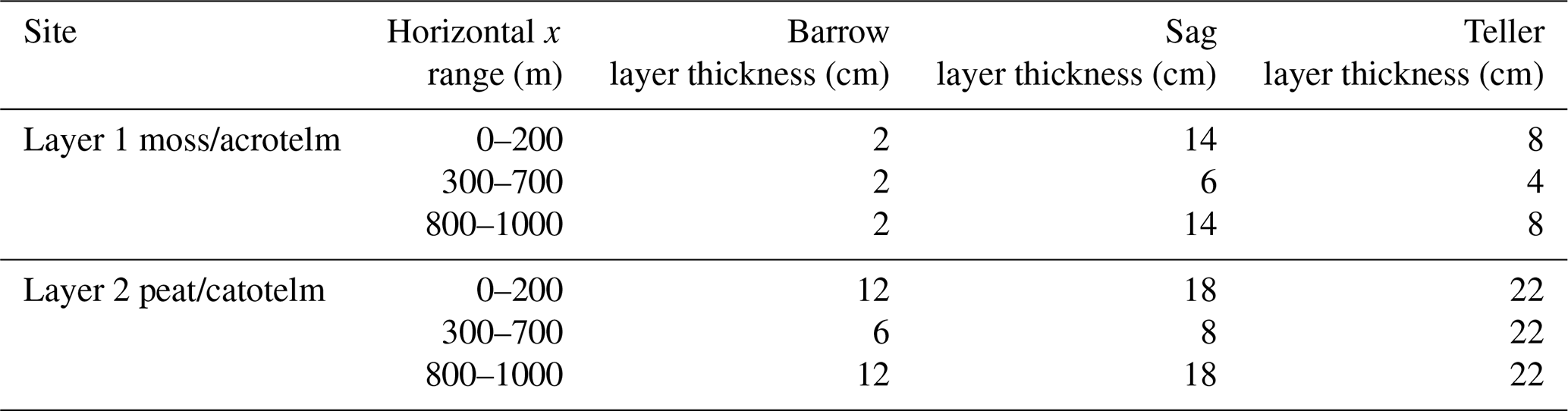
In the hillslope scenario, we designed the mesh based on observations at Teller to represent a generalized, varying-thickness low Arctic hillslope. A hillslope mesh was created first by generating a pseudo-2D surface mesh with 50 cells and then extruding the 2D mesh downward by 50 m. The pseudo-2D surface was designed in a trapezoidal shape with a single, variable-width cell in the cross-slope direction to represent convergent/divergent hillslopes, the short and long sides of which are 200 and 800 m, respectively (see Fig. 3). Vertically, from the surface downward, the grid size distribution was the same as the column mesh for each site. The domain is also composed of three layers, the same as the column, while the numbers of cells representing each soil layer (i.e., soil layer thickness) are different along the hillslope. The thickness distribution of the first two layers of each site is shown in Table 3. The third layer of a hillslope for all sites is the principal mineral soil. Additionally, hillslope meshes with different aspects (i.e., north-facing, south-facing) were also created.

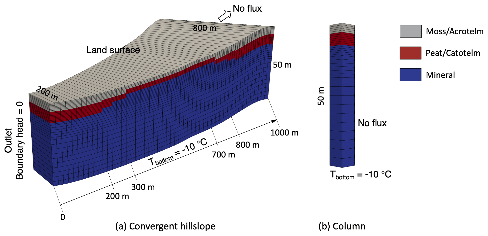
Figure 3 Schematic domain mesh and soil layer partition: (a) example of a convergent hillslope domain and (b) column domain.

Table 3 Thickness distribution of the organic layers along hillslope for each site.

3.3 Model setup

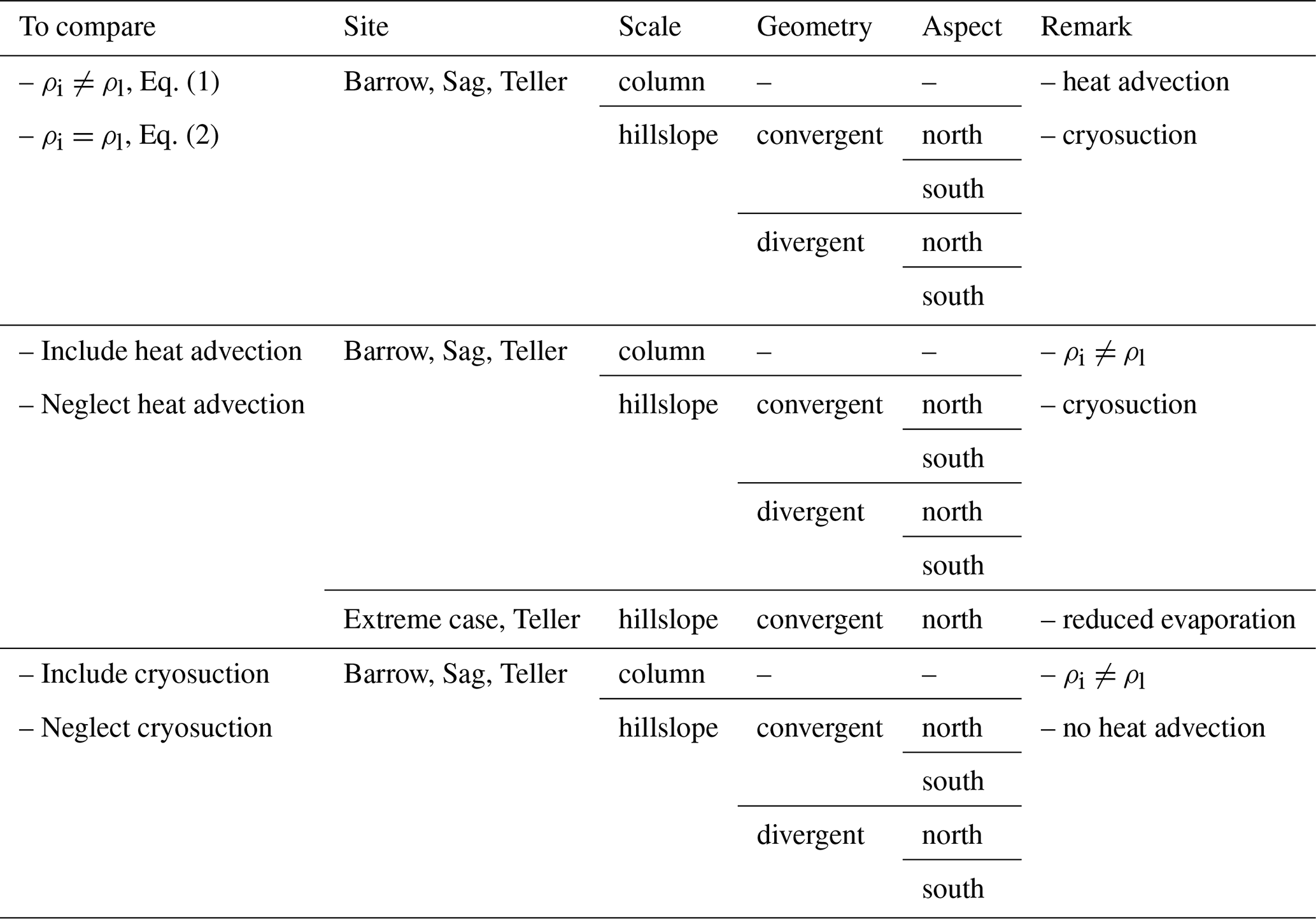
To study how the representations of the three physical processes (i.e., ice expansion represented by density, cryosuction, and advective heat transport) affect simulated hydrological outputs at different scales and hillslope topography features, as well as under various forcing and soil conditions, 62 model simulations were conducted, summarized in Table 4. To examine the validity of the assumption of equal density between ice and liquid water, we included cryosuction and advective heat transport in models. To investigate the role of cryosuction in permafrost modeling, we used a different density while neglecting advective heat transport to decrease the computation cost. Note that neglecting advective heat transport in these runs can reduce the effect of cryosuction on simulation predictions, as cryosuction moves water which would itself advect energy. To compare the difference between neglecting and including heat advection, we used different density expressions for ice and liquid and included cryosuction. Particularly, in order to understand the impact of advective heat transport on permafrost processes when soil is at its wettest, we designed two extreme cases under the warm, wet conditions of the Teller site in which soil evaporation was artificially reduced. These runs were designed to maximize water flux and therefore maximize the potential for advective heat transport to affect predictions.

Table 4 Ensemble of models designed in this study.

Prior to simulating all cases, two steps of initialization are carried out for each site. First, a column model initially above freezing temperature with a given water table depth was frozen by setting the bottom temperature at a constant value of −10 ^∘C until a steady-state frozen soil column is formed. The initial water table depth is chosen to ensure that the frozen column's water table, after accounting for expansion of ice, is just below the soil surface. The pressure and temperature profiles of the frozen column were used as the initial conditions of the second step initialization. Before proceeding, the observed forcing data (period of 2011–2020) was averaged across the years to form a 1-year, “typical” forcing year, which was then repeated 10 times. Using this typical forcing data and the solutions of the first step, we solved the column model in a transient solution, calculating an annual cyclic steady state. The final pressure and temperature profile of the column at the end of the 10-year simulation was then assigned to each column of the hillslope mesh as the initial condition in the formal simulations listed in Table 4. The temperature at the bottom was constant at −10 ^∘C.

3.4 Evaluation metrics

To fully assess the effect of representation of ice density, advective heat transport, and cryosuction in permafrost hydrology modeling, we used the root mean squared error (RMSE) and normalized Nash–Sutcliffe efficiency (NNSE) as performance metrics. RMSE has the same dimension as the corresponding variables, which can be used to evaluate the average absolute deviation from a benchmark, defined by

$$\begin{array}{}\text{(7)}& \mathrm{RMSE}=\sqrt{{\displaystyle \frac{{\sum }_{t=\mathrm{1}}^N{\left(x_t-y_t\right)}^{\mathrm{2}}}{N}}},\end{array}$$

where x_t and y_t are the two modeled datasets to compare from the initial time point (t=1) to the end (t=N).

NNSE is a normalized dimensionless metric describing the relative relationship between an estimation and a reference, which is oftentimes used for evaluating hydrological models:

$$\begin{array}{}\text{(8)}& \mathrm{NNSE}=\mathrm{1}/\left(\mathrm{1}+{\displaystyle \frac{{\sum }_{t=\mathrm{1}}^N{\left(x_t-y_t\right)}^{\mathrm{2}}}{{\sum }_{t=\mathrm{1}}^N{\left(x_t-\stackrel{\mathrm{‾}}{x}\right)}^{\mathrm{2}}}}\right),\end{array}$$

where the modeled results x_t (obtained without physics simplification) are considered as the benchmark, and $\stackrel{\mathrm{‾}}{x}$ is the mean value of the benchmark. A NNSE approaching 1 indicates perfect correspondence between two groups of values in comparison.

In addition, we also used the normalized mean absolute error (MAE) to quantify the percentage change of results obtained with simplified physics relative to full physical representations (see Sect. 4.4):

$$\begin{array}{}\text{(9)}& \mathrm{Normalized}\mathrm{MAE}={\displaystyle \frac{\sqrt{{\sum }_{t=\mathrm{1}}^N\left|x_t-y_t\right|/N}}{\mathrm{normalizing}\mathrm{reference}}}\times \mathrm{100}\mathit{\%}.\end{array}$$

Two normalizing references were selected considering different modeled metrics of interest. For instance, in terms of temperature and saturation which fluctuate between two non-zero values, the annually averaged variation range was chosen as the reference.

$$\mathrm{Normalizing}\mathrm{reference}={\displaystyle \frac{{\sum }_{\mathrm{year}=\mathrm{1}}^{\mathrm{num}\mathrm{of}\mathrm{years}}\left(\mathrm{maximum}-\mathrm{minimum}\right)}{\mathrm{number}\mathrm{of}\mathrm{years}}}$$

For a modeled metric with zero as the smallest value, such as evaporation, discharge, and thaw depth, the corresponding average value was selected as the reference.

4 Results

This section compares simulated outputs over the period of 2011–2020 for the three physical processes under different simulating conditions. We focus on the impact on integrated metrics, such as evaporation, discharge, and averaged thaw depth, and depth-dependent metrics, such as temperature and total water saturation (ice and liquid). For hillslope models, we chose five surface locations according to the slope geometry to collect simulated data, which were then averaged to obtain a single outcome for each metric of interest.

4.1 Ice density

To evaluate the representation of ice density on permafrost process simulation, we compared evaporation, discharge, thaw depth, and total water saturation between simulations using equal and different ice density expressions. Figures 4 and 5 show an example of the comparison under conditions of Sag at column and hillslope scales, respectively. Results are compared in both time series and correlation.

Generally, at both column and hillslope scales, assuming equal density between ice and liquid has minor impacts on evaporation, discharge, and thaw depth over the 10-year simulation, except at a few deviated points as shown in the correlation figures. According to column-based models, the RMSEs of evaporation, discharge, and thaw depth are 0.101 mm d⁻¹, 0.001 m³ d⁻¹, and 1.648 cm, respectively, 1 order of magnitude smaller than the values of the corresponding metrics. At the hillslope scale (see Fig. 5) the south-facing divergent hillslope is selected to show the modeling comparison on evaporation and thaw depth in that they are potentially mostly affected when a hillslope has a south orientation and divergent geometry. Likewise, the north-facing convergent hillslope is chosen to compare discharge and water saturation from simulations with different density expressions. Even then, RMSEs of the three metrics are 0.064 mm d⁻¹, 111.073 m³ d⁻¹, and 0.825 cm, respectively, 2 orders of magnitude smaller than the values of the corresponding metrics at the hillslope scale. Besides, NNSEs of the three metric outputs from both column and hillslope simulations are over 0.9, approaching 1 especially at the hillslope scale. Therefore, all indicate good performance of the equal ice–liquid density assumption in predicting integrated metrics and thaw depth. By comparison, the estimation of water saturation is relatively more affected by the density assumption during cold seasons within a year, as shown by Figs. 4d and 5d. This is reasonable in that when water mainly exists in the form of ice, equal ice–liquid density assumption will overestimate the water content.

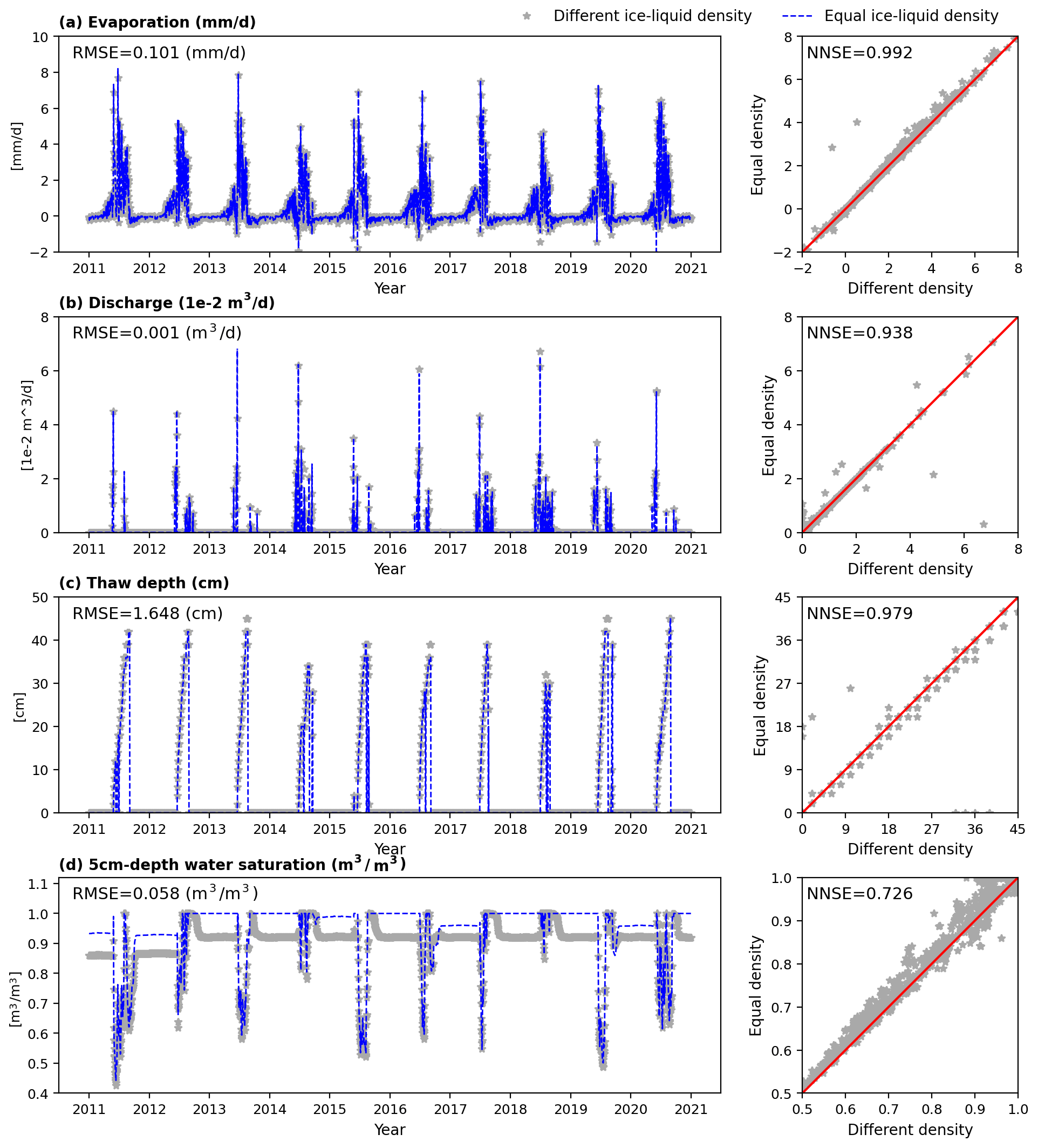
Figure 4 Comparison of column simulations between different and equal ice–liquid density under conditions of Sag in (a) evaporation, (b) discharge, (c) thaw depth, and (d) water saturation at 5 cm beneath the surface from year 2011 to 2020.

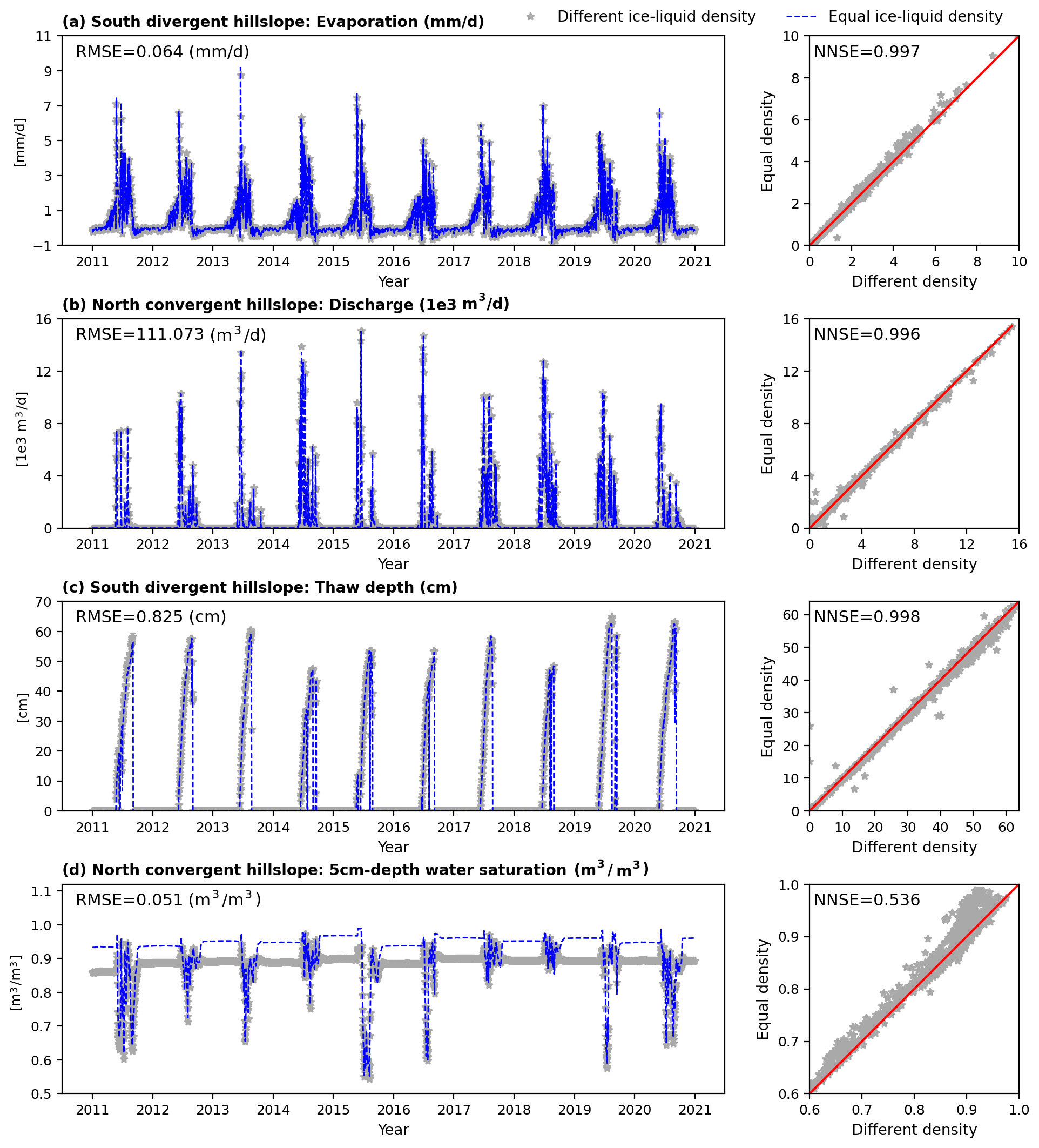
Figure 5 Comparison of hillslope simulations between using different and equal ice–liquid density under conditions of Sag in (a) evaporation, (b) discharge, (c) thaw depth, and (d) water saturation at 5 cm beneath the surface from year 2011 to 2020.

4.2 Cryosuction

To evaluate the effect of cryosuction on permafrost process predictions, we compared evaporation, discharge, thaw depth, total water saturation, and temperature obtained through simulations including and neglecting cryosuction. Figure 6 through Fig. 8 illustrate column-scale comparisons of these metrics under conditions at the three sites (Barrow, Sag, and Teller). Figure 6 presents the effect of excluding cryosuction on evaporation and discharge. The RMSE of evaporation from the three sites ranges between 0.25 and 0.35 mm d⁻¹, still 1 order of magnitude smaller than the common evaporation rate. Evaporation NNSEs of the three sites are around 0.9. For discharge, RMSEs are also 1 order of magnitude smaller than the average, whereas NNSEs fall between 0.6 and 0.9. Generally, cryosuction plays a more important role in predicting discharge compared to evaporation, especially under warm and wet climate conditions, such as at Teller.

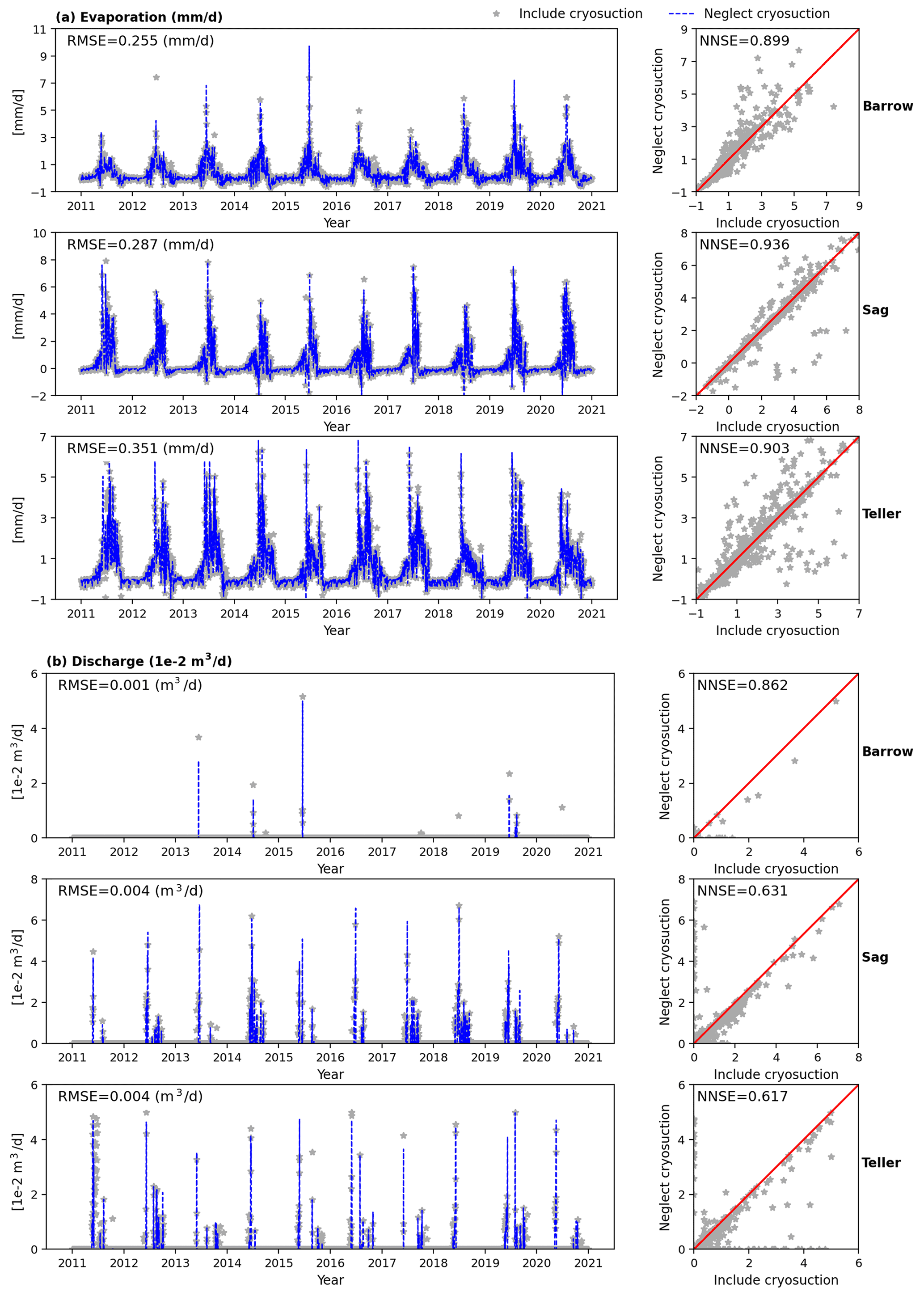
Figure 6 Comparison of column simulations between including and neglecting cryosuction under conditions of Barrow, Sag, and Teller in (a) evaporation and (b) discharge.

Figure 7 shows the effect of cryosuction on column-scale simulated thaw depth and total water saturation at 5 cm beneath the surface. Overall, neglecting cryosuction tends to underestimate the deepest thaw depth. As already mentioned, cryosuction, in essence, increases soil suction to attract more liquid water moving towards the frozen front during soil freezing. Thus, the real active layer formed due to the existence of cryosuction should be thicker than the cases in which cryosuction is assumed unimportant. RMSEs of thaw depth in Fig. 7 range from 3 to 8 cm. Though still 1 order of magnitude smaller than the average annual thaw depth, the estimation error due to neglecting cryosuction is most obvious in summer, especially at areas with cold temperature like Barrow. By comparison, at Teller, where the largest thaw depth is over double that of Barrow and Sag due to its higher temperature, soil cryosuction does not essentially affect thaw depth compared to the other two sites. Similarly, for the total water saturation, at Barrow, the effect of cryosuction is more clearly observed, not only during cold seasons as observed for density representation (Sect. 4.1) but also in summers. The reason why Barrow is more sensitive to the cryosuction process on predicting thaw depth and water content is determined by both soil properties and climate conditions. The soil at Barrow has larger suction and is able to hold more water (see Fig. 2), providing the possibility for cryosuction to make contributions. Moreover, the principal difference between cryosuction and non-cryosuction representations is presented when the temperature is below the freezing point (see Eqs. 3 and 4). Compared to Sag and Teller, Barrow has lower annual average temperature (see Fig. 1), making the effect of cryosuction more pronounced.

Figure 7 Comparison of column simulations between including and neglecting cryosuction under conditions of Barrow, Sag, and Teller in (a) thaw depth and (b) water saturation at 5 cm beneath the surface.

Finally, we also compared soil temperature obtained from models with and without cryosuction in Fig. 8. Surface temperature is little affected by cryosuction, except at the Sag site, where the surface temperature is overestimated during winter. At 1 m depth, the soil temperature of Barrow is slightly changed in summer due to neglecting cryosuction. At both Sag and Teller, the fluctuation range of temperature at 1 m beneath the land surface is underestimated if the cryosuction effect is not considered, especially at Sag, and NNSE decreases to approximately 0.6. The reason why Sag and Teller are more sensitive to the effect of cryosuction on temperature is associated with the larger water volume at the two sites. During freezing, soil freezes from the ground surface downward and from the bottom of the active layer upward, forming a liquid zone in between where the temperature approximates the freezing point due to phase change (Fig. S3.1a in the Supplement shows an example of the column model under the Sag River condition at the 300th day of one year). Thus, this liquid zone isolates the upper permafrost from the soil surface temperature variations due to the weakened conductive heat transport along the soil depth. Additionally, the released latent heat in this liquid zone may retard soil freezing, which also tends to reduce thermal conduction. However, cryosuction can speed up freezing and promote the attenuation of the liquid zone (see Fig. S3.1a and b. Figure S3.1b shows the ice saturation at the same time as Fig. S3.1a, when a soil column still has a large non-frozen area), which thus decrease the impact of the liquid zone. Hence, the influence of cryosuction is more significant with more soil water.

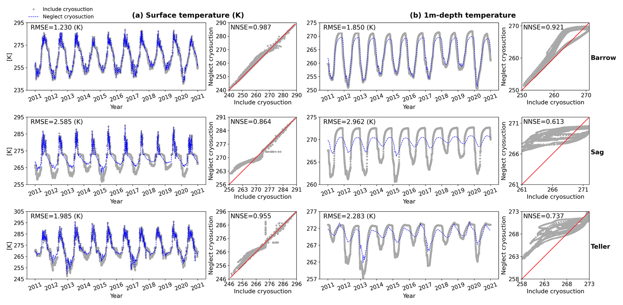
Figure 8 Comparison of column simulations between including and neglecting cryosuction under conditions of Barrow, Sag, and Teller in (a) surface temperature and (b) temperature at 1 m beneath the surface.

Therefore, from Fig. 6 to Fig. 8, neglecting the cryosuction effect in column-scale simulations has less impact on integrated hydrological metrics but will cause significant difference when estimating thaw depth and location-specific metrics. The difference among these metrics varies under different climate conditions. Integrated metrics, such as evaporation and discharge, are affected more under warm and wet conditions (Teller); thaw depth and water saturation are affected more under cold and low-rainfall conditions (Barrow); and soil temperature tends to be affected more under cold and high-precipitation (rain and snow) conditions (Sag).

Neglecting soil cryosuction has a similar impact on hydrological outputs in hillslope-scale models. Figure 9 shows the comparison of the metrics of interest discussed above under the Sag climate. Evaporation, thaw depth, and temperature are presented based on south-facing divergent hillslope models, while discharge and water saturation are from hillslope models with a north-facing convergent geometry. In general, neglecting soil cryosuction has a smaller effect on integrated metrics (evaporation and discharge) compared with other pointwise metrics. Though thaw depth presents a high NNSE of approximately 0.94 and low RMSE of about 4.5 cm compared to the average, indicating a good match between models considered and excluded cryosuction, the estimation error during summer may reach as high as 10 cm, particularly from 2011 to 2017, as shown in Fig. 9c. Obvious errors in water saturation and temperature, similar with column-scale models, occur almost annually with respect to extrema during winter and summer. Overall, compared to column-scale models, differences in evaporation, discharge, thaw depth, and surface temperature due to neglecting cryosuction are relatively reduced at the hillslope scale if comparing NNSEs (Table 5). Localized subsurface metrics, such as water saturation and 1 m depth soil temperature, show increased errors from column- to hillslope-scale models, which is primarily caused by lateral flux exchange captured by hillslope modeling.

Figure 9 Comparison of hillslope simulations between including and neglecting cryosuction under conditions of Sag in (a) evaporation, (b) discharge, (c) thaw depth, (d) water saturation at 5 cm beneath the surface, (e) surface temperature, and (f) temperature at 1 m beneath the surface.

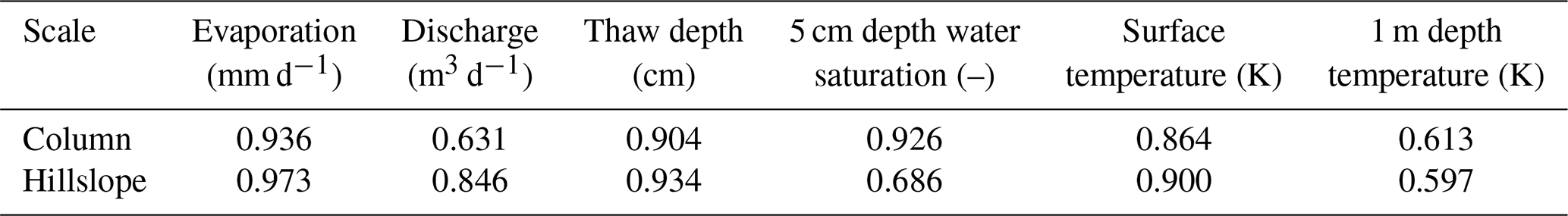
Table 5 NNSE of outputs from column and hillslope models under conditions of Sag shown in Fig. 6 through Fig. 9.

4.3 Advective heat transport

This section evaluates the performance of advective heat transport in modeling the permafrost process. As above, we investigated the influence of neglecting heat advection on evaporation, discharge, thaw depth, total water saturation, and temperature. Overall, after comparing all hydrological outputs from models with different heat transport representations, heat advection is proved insignificant in an Arctic system where the influence of localized groundwater flow can be neglected. Comparisons based on column-scale and hillslope-scale models are not shown here (see Supplement); instead, the extreme case under conditions of Teller is presented (Fig. 10). Teller is abundant in rainfall over the period of 2011–2020 (Fig. 1). In the extreme case, evaporation was reduced artificially to almost a quarter of the original value (see Fig. 6a at Teller and Fig. 10a) for the purpose of increasing water flow rates. For instance, discharge has quadrupled after adjusting evaporation by comparing Fig. 10b and Fig. 6b at Teller. This specific scenario is chosen to maximize the potential effect of advective heat transport in a hillslope-scale Arctic system. Figure 10 illustrates comparisons on all outputs mentioned above from hillslope models without heat advection and with full thermal representation. Apparently, all RMSEs are extremely small, at least 2 orders of magnitude lower than the corresponding metric average. Almost all NNSEs are approximately 1, even for thaw depth, localized water saturation, and temperature. Under the assumption of large-scale Arctic systems ignoring the influence by localized groundwater flow features (e.g., ponds, gullies), the liquid water flux determines the advective heat transport in the subsurface. However, the flow velocity on average is quite low within the shallow active layer with limited thickness (see Fig. S4.1). As a consequence, the advective heat transport only makes contributions within the top shallow layers, and the relatively larger advective heat flux is lower than the conductive heat flux over 1 order of magnitude (see Fig. S4.2). Therefore, for such large-scale Arctic systems where localized groundwater flow makes less of a contribution, it is reasonable to neglect advective heat transport.

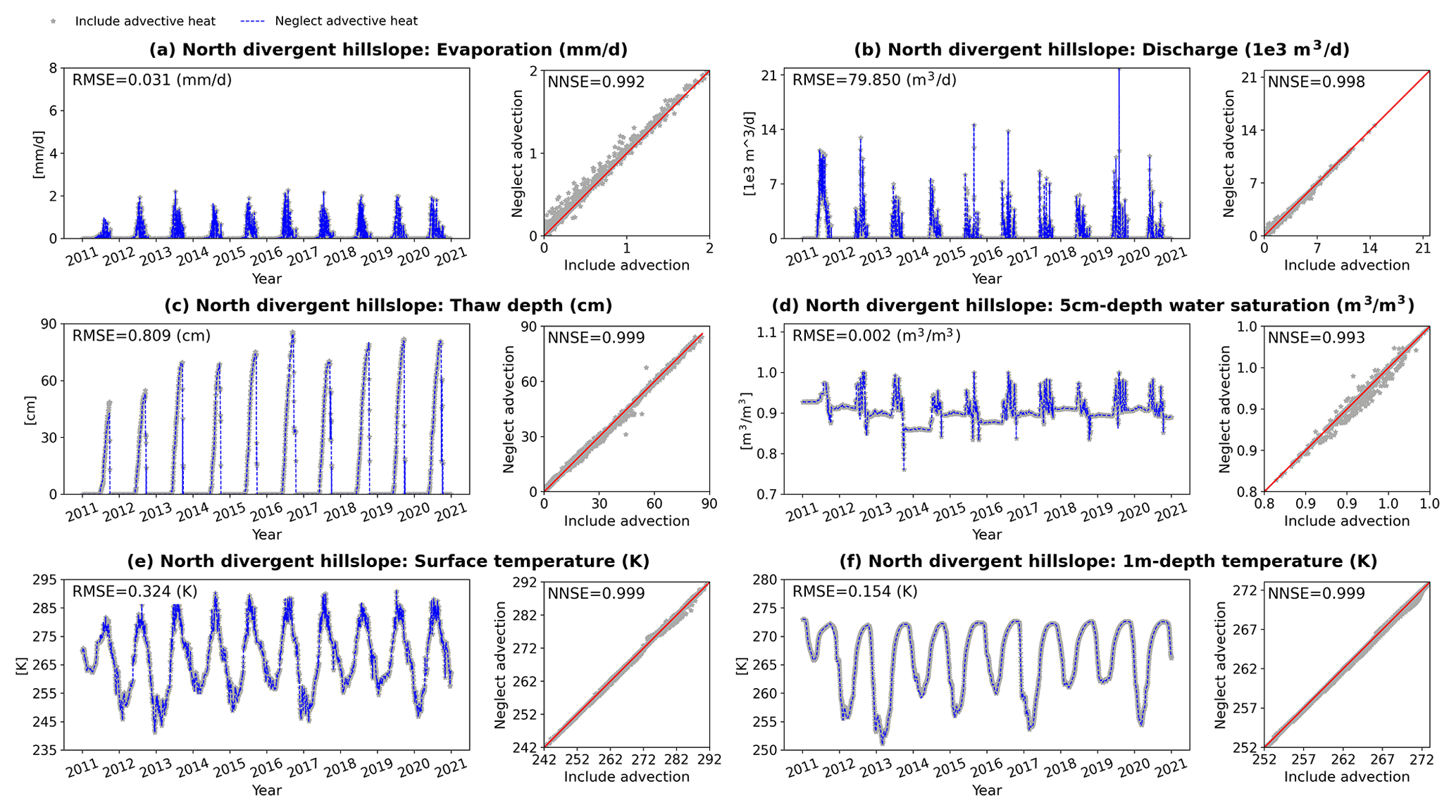
Figure 10 Comparison of hillslope simulations between including and neglecting advective heat transport under extreme conditions of Teller in (a) evaporation, (b) discharge, (c) thaw depth, (d) water saturation at 5 cm beneath the surface, (e) surface temperature, and (f) temperature at 1 m beneath the surface.

4.4 Comprehensive comparison

In the above three sections, we discussed time-series simulation comparisons. This section will analyze the effect of equal ice–liquid density, neglecting cryosuction, and neglecting heat advection on permafrost modeling outputs from holistic, average perspectives.

First, we extracted NNSEs of all the metrics of interest obtained from all comparing models for qualitative analysis. Table 6 shows an example based on column-scale models under the conditions of the three different sites. Red numbers highlight the obviously reduced NNSEs of one or two processes among the three for each metric. Overall, neglecting advective heat transport has the least influence on model outputs. Equal ice–liquid density primarily affects saturation and has less effect on other metrics. Excluding soil cryosuction makes the greatest impact on almost all metrics, especially in a relatively wet environment. Among these metrics, evaporation and surface temperature are less affected by the three physical process representations, while location-based water saturation is most affected.

Table 6 A summary of NNSEs of metrics of interest obtained through column model comparison.

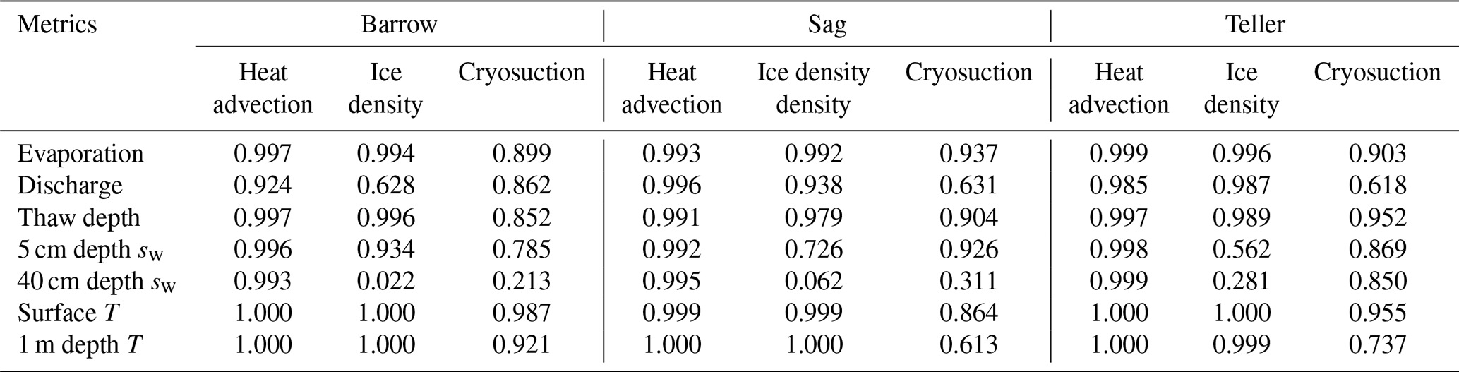
Note: s_w and T in Table 6 are water saturation and temperature, respectively.

Furthermore, to quantitively compare across the physical processes, we calculated the mean absolute error (MAE) for each metric of interest over the simulation period of 2011–2020. For evaporation, discharge, and thaw depth, the MAEs are normalized by the corresponding metric average (numbers in Fig. 11a); for water saturation and temperature, the MAEs are normalized by their average annual fluctuation range (numbers in Fig. 11b). All normalized MAEs are presented in percentage, displayed in Fig. 11 according to column- and hillslope-scale (e.g., south-facing convergent hillslope) models under three different climate conditions. The hillslope-scale model output under the conditions of Barrow is not shown in that a majority of the area is flat land. A larger normalized MAE percentage indicates that the greater impact on the metric resulted from a physical process.

From the perspective of a 10-year average, in general, each physical process of Arctic systems discussed in this paper presents a similar impact on metrics between column and hillslope scales. Under climate and soil conditions of three different sites, neglecting cryosuction in permafrost modeling leads to the greatest influence on hydrological prediction amongst the three physical assumptions. As seen in Fig. 11a, it will result in 10 %–20 % deviation in evaporation, 50 %–60 % in discharge, and 10 %–30 % in thaw depth. Evaporation is the least affected among the three metrics. Discharge is more affected in regions with abundant rainfall (Teller), while in regions with less precipitation, evaporation and thaw depth are relatively affected (Barrow). By comparison, assuming equal ice–liquid density and neglecting advective heat transport may only cause 10 % and 5 % or even much lower error, respectively, in reference to the annual average of a metric. Especially in Barrow, models utilizing the same ice and liquid densities and ignoring advective heat transport seem to make an obvious impact on discharge, whereas this also results from its extremely low discharge (Fig. 6b).

Figure 11b illustrates the normalized MAEs of water saturation at 5 cm beneath the surface, as well as temperature at the surface and 1 m depth. The assumption of equal ice–liquid density primarily affects the estimation of the water saturation profiles, which can lead to about 5 %–15 % error relative to the annual change range, and the error percentage tends to slightly decrease when applying hillslope-scale models due to the inclusion of lateral flow. Apart from this, neglecting soil cryosuction still makes the largest impact. Surface temperature is the least affected metric among all these model outputs even if cryosuction is not included in modeling. However, at 1 m depth, error can increase to 10 %–30 % by simulation without cryosuction representation.

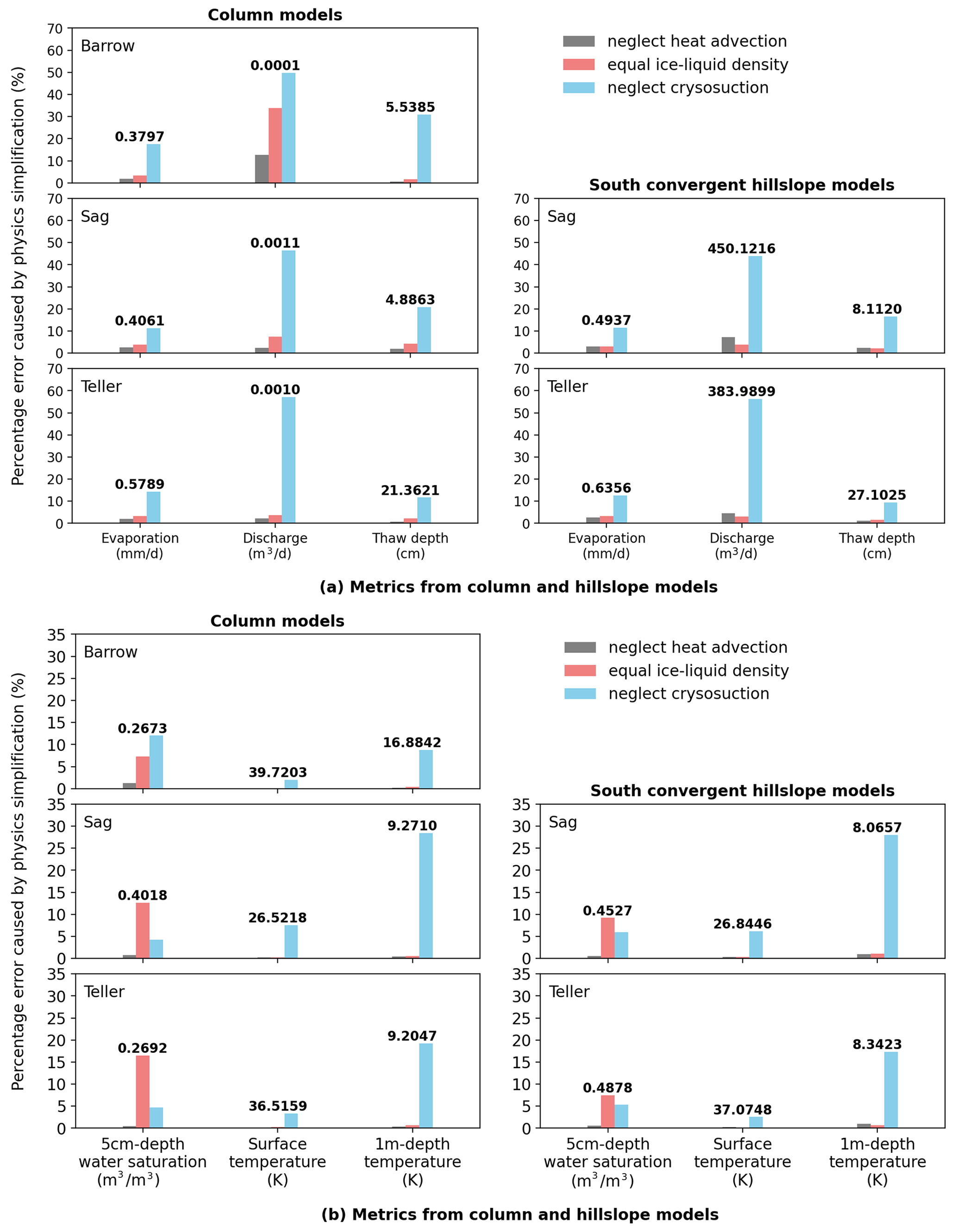
Figure 11 Percentage errors for each metric caused by physics simplifications at column and hillslope scales. The percentage error refers to the averaged error of a metric over the period of 2011–2020 normalized by a certain reference value obtained from the full-physics model. Metrics include (a) evaporation, discharge, and thaw depth and (b) water saturation and temperatures. Numbers in figures are the corresponding reference values for each metric: (a) 10-year average obtained from the full-physics model; (b) 10-year averaged annual fluctuation range obtained from the full-physics model.

5 Conclusions

The premise of this study is that, by starting from general mass and energy transport equations and simplifying the process representations, we can use a process-rich model to understand the relative importance of given process simplifications in describing permafrost hydrology. This process sensitivity analysis, performed at the scale of field sites as opposed to previous studies at smaller scales such as lab experiments, provides improved understanding in the processes governing permafrost hydrology at this scale. As the simplifications considered here largely span the equations considered in a class of process-rich models, this process sensitivity analysis is relevant to model developers across a range of codes.

Simplification of Arctic process representation is an essential consideration when developing process-rich models for thermal permafrost hydrology. The following three subsurface process simplifications are commonly applied for many Arctic tundra models: (i) ice is prescribed the same density as liquid water, (ii) the effect of soil cryosuction is neglected, and (iii) advective heat transport is neglected. Here we investigated the influence of these simplified representations on modeling field-scale permafrost hydrology in a set of simplified geometries commonly used in the permafrost hydrology literature with the Advanced Terrestrial Simulator (ATS v1.2). We note that these conclusions are specific to conditions similar to these geometries and should not be applied in cases in which focusing flow mechanisms may dominate.

To do this, we conducted an ensemble of simulations to evaluate the impact of the above three process simplifications on field-scale predictions. The ensemble of simulations consisted of 62 numerical experiments considering various conditions, including different climate conditions and soil properties at the three sites of Alaska, and different model-scale conceptualizations. For evaluation, we compared integrated metrics (evaporation, discharge), averaged thaw depth, and pointwise metrics (temperature, total water saturation), which are of general interest, among different models to access the deviation of applying a simplified modeling assumption. The main conclusions, under the assumed conditions in this study, are summarized as follows.

1. Excluding soil cryosuction can cause significant bias on the estimation of most hydrological metrics at field-scale permafrost simulations. In particular, under the assumed conditions, the average deviation in evaporation, discharge, and thaw depth may reach 10 %–20 %, 50 %–60 %, and 10 %–30 %, respectively, relative to the corresponding annual average values. The prediction error for discharge may grow if rainfall rates increase. In the case of pointwise metrics, the error in temperature increases from a small amount at the surface up to 10 %–30 % at 1 m beneath the surface. The prediction of subsurface temperature and water saturation is especially affected when considering hillslope-scale models. Therefore, soil cryosuction should be included when modeling permafrost change.

2. Assuming equal ice–liquid density will not result in especially large deviations when predicting most of the hydrological metrics, particularly at hillslope scales given all cases in this study. It primarily affects the prediction of the soil water saturation profile and can cause 5 %–15 % error relative to the annual saturation fluctuation range. This difference may have consequences for the carbon cycle with regards to the production of methane versus carbon dioxide. Assigning liquid water density for ice may reduce computational time to a small extent in ATS, dependent on simulating conditions and spatial and temporal scales.

3. For a large-scale Arctic tundra system with limited localized groundwater flow features (e.g., taliks, thermo-erosion gullies), the prediction error in most metrics of interest after neglecting advective heat transport is less than 5 % or even much lower. In the case of ATS, the simulation time cost for hillslope-scale models can decrease by 40 % to 80 % under conditions in this study. Ignoring heat advection in the absence of local, flow-focusing mechanisms, such as thermo-erosion gullies, seems a reasonable decision.

Through the comparison of permafrost hydrological outputs obtained from ensemble model setups targeted at the field scale, we confirm the importance and necessity of including soil cryosuction in predicting permafrost changes and validate the application of equal ice–liquid density and neglecting advective heat transport for an Arctic system where localized groundwater flow is not a dominant feature. The latter two may also ease computational cost dependent upon simulation conditions. We expect that this study can contribute to the development of permafrost hydrology models, as well as better selection of physical process representations for modelers, and a better understanding of permafrost physics for the community.

Appendix A

The following results may provide some information about computation cost for ATS users. In addition to the influence of process representations on permafrost hydrology metrics of general interest, we also investigated how much the simplified processes can affect the runtime of a model at the hillslope scale.

First, using the 10-year simulation with real ice density as references, the percentage change of time consumed after applying equal ice–liquid density was calculated and is displayed in Fig. A1. Overall, under the equal density assumption, it may take less time (positive values in figure) but no more than 25 % and on average lower than 10 %. However, the computation time may also increase (negative values in figure) under wet conditions, such as at Sag and Teller. Thus, given a long-period modeling of a large-scale permafrost system, there is no consistent conclusion on whether equal ice–liquid density can ease computational cost. It depends on both the weather conditions and soil properties.

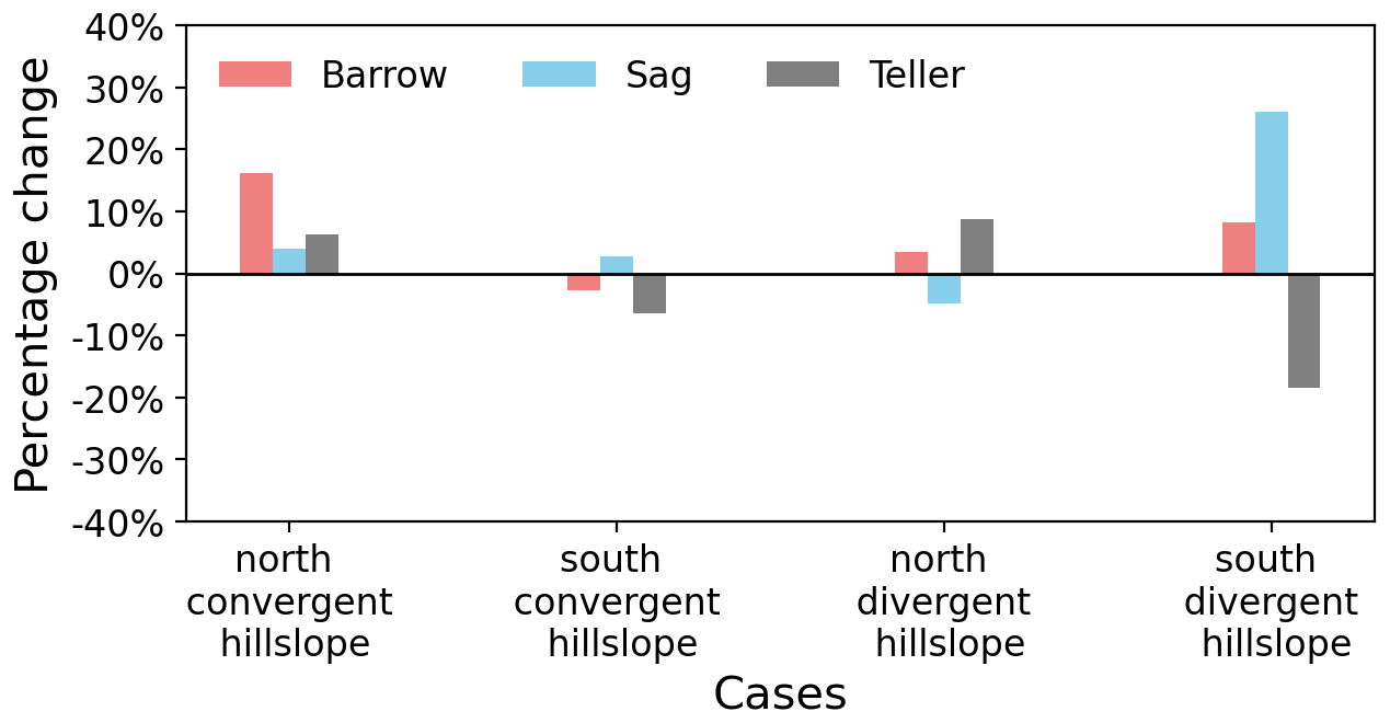
Figure A1 The relative runtime change in percentage due to the assumption of equal ice–liquid density compared to that with the real ice density representation for all hillslope-scale models.

Second, Sect. 4.2 has demonstrated that neglecting cryosuction will make a great impact on hydrological estimations. As a significant physical process of permafrost, cryosuction should be implemented in numerical models even if additional computation effort is potentially required. However, based on the hillslope models we conducted, including cryosuction does not necessarily raise computational cost, which also depends on specific soil properties and conditions. The cases that consume more time after considering the cryosuction effect just increase the time by 10 %–30 % and less than 20 % on average (see Fig. A2).

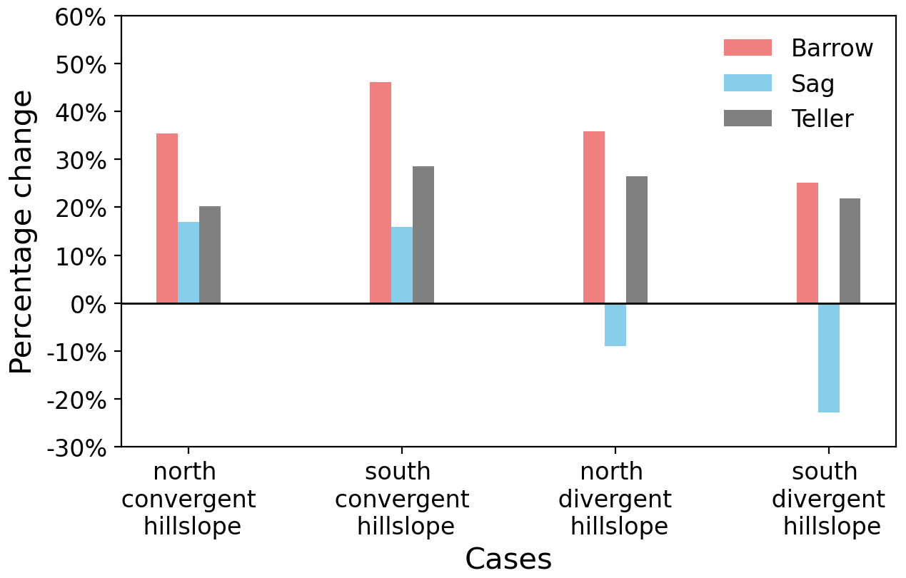
Figure A2 The relative runtime change in percentage after neglecting cryosuction compared to the cases with cryosuction for all hillslope-scale models.

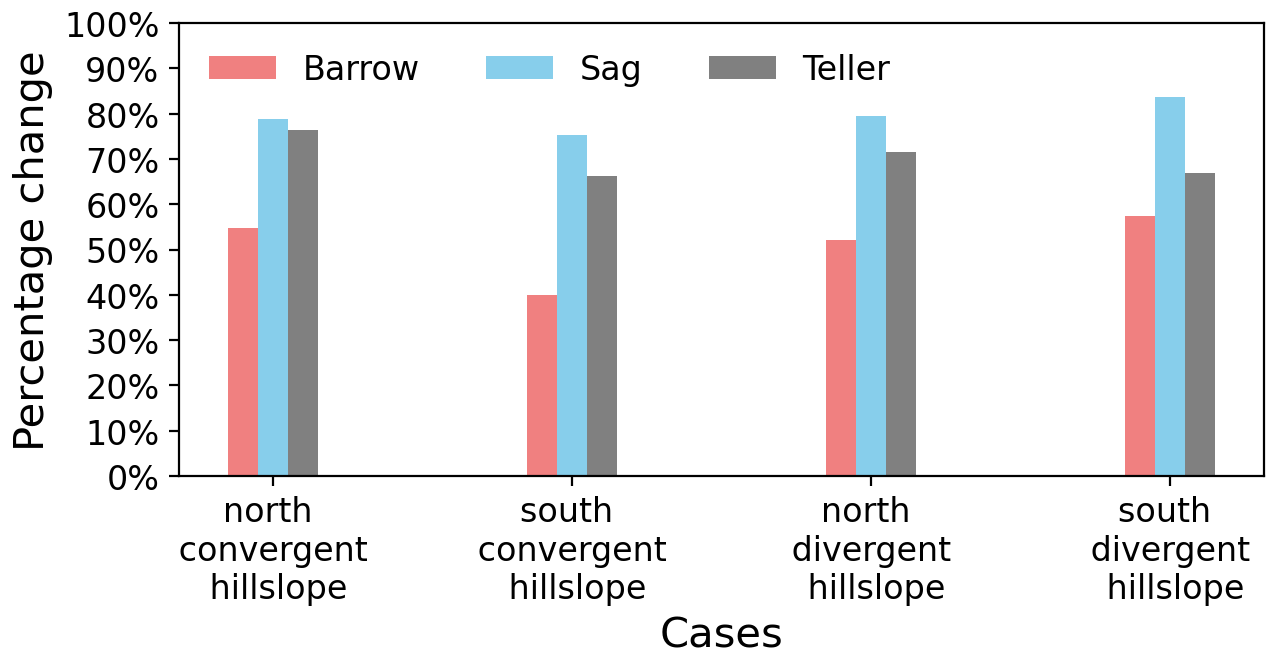
Figure A3 The relative runtime change in percentage due to the neglect of advective heat transport for all hillslope-scale models.

Third, in terms of heat advection, ATS uses the algebraic multigrid method as preconditioner for solving, which has a relatively deficient performance in dealing with hyperbolic equations. Thus, incorporating advective heat transport will aggravate computational cost, particularly in the case of both large spatial and temporal scales. Figure A3 shows the relative percentage reduction in computational time for 10-year simulations after excluding heat advection in both surface and subsurface thermal flux. It drops by 70 %–80 % under wet conditions (e.g., Sag and Teller) and 40 %–60 % under dry conditions (e.g., Barrow). Hence, neglecting advective heat transport considerably improves the performance of large spatial-temporal permafrost hydrology simulations.