the Creative Commons Attribution 4.0 License.
the Creative Commons Attribution 4.0 License.
 | 10 Oct 2022
On the evolution of an ice shelf melt channel at the base of Filchner Ice Shelf, from observations and viscoelastic modeling
Julia Christmann
Hugh F. J. Corr
Veit Helm
Lea-Sophie Höyns
Coen Hofstede
Ralf Müller
Niklas Neckel
Keith W. Nicholls
Timm Schultz
Daniel Steinhage
Michael Wolovick
Ole Zeising
Ice shelves play a key role in the stability of the Antarctic Ice Sheet due to their buttressing effect. A loss of buttressing as a result of increased basal melting or ice shelf disintegration will lead to increased ice discharge. Some ice shelves exhibit channels at the base that are not yet fully understood. In this study, we present in situ melt rates of a channel which is up to 330 m high and located in the southern Filchner Ice Shelf. Maximum observed melt rates are 2 m yr−1. Melt rates inside the channel decrease in the direction of ice flow and turn to freezing ∼55 km downstream of the grounding line. While closer to the grounding line melt rates are higher within the channel than outside, this relationship reverses further downstream. Comparing the modeled evolution of this channel under present-day climate conditions over 250 years with its present geometry reveals a mismatch. Melt rates twice as large as the present-day values are required to fit the observed geometry. In contrast, forcing the model with present-day melt rates results in a closure of the channel, which contradicts observations. The ice shelf experiences strong tidal variability in vertical strain rates at the measured site, and discrete pulses of increased melting occurred throughout the measurement period. The type of melt channel in this study diminishes in height with distance from the grounding line and is hence not a destabilizing factor for ice shelves.
- Article
(11643 KB) - Full-text XML
- BibTeX
- EndNote


Melt channels carved upward into the base of ice shelves have been hypothesized to destabilize ice shelves and are often linked to enhanced basal melt (Le Brocq et al., 2013; Langley et al., 2014; Drews, 2015; Marsh et al., 2016; Dow et al., 2018; Hofstede et al., 2021a). At some locations, these channels increase in height with distance from the grounding line, thus reducing the structural strength of the ice shelf, while at other locations they diminish downstream, minimizing their influence on shelf integrity. It remains unknown why some channels diminish downstream and whether channels that diminish downstream are also locations of enhanced basal melt.
Channels at the base of ice shelves may form where subglacial channels beneath the inland grounded ice discharge fresh water into the ocean (Le Brocq et al., 2013), or they may arise from topographic features or from shear margins developing surface troughs when adjusting to flotation (Alley et al., 2019). Features like bedrock undulations or eskers underneath the grounded ice may also leave a channel-like imprint in the geometry of the floating shelf (Drews et al., 2017; Jeofry et al., 2018). In all cases, the geometry of the channel at the ice base is altered by two factors: incision due to basal melt arising from oceanic heat and closure due to viscoelastic creep.
Surface troughs on ice shelves are linked to incisions at the ice base, thus either to melt channels (e.g., Le Brocq et al., 2013; Langley et al., 2014) or to basal crevasses (e.g., Humbert et al., 2015). The surface troughs are formed by viscoelastic deformations in the transition to buoyancy and buoyancy equilibrium itself. Channels at the ice base have been surveyed using radio echo sounding (Rignot and Steffen, 2008; Vaughan et al., 2012; Le Brocq et al., 2013; Dutrieux et al., 2014; Langley et al., 2014; Dow et al., 2018). Their typical dimensions range from 300–500 m wide and up to 50 m high (Langley et al., 2014) to 1–3 km wide and 200–400 m high (Rignot and Steffen, 2008). Channel flanks are not necessarily smooth but may form terrace structures in the lateral (across ice flow) dimension as shown by Dutrieux et al. (2014) for Pine Island Glacier, Antarctica. These terraces are separated by up to 50 m high walls with steep slopes between 40 and 60∘.
Hofstede et al. (2021a) found a basal channel on Support Force Glacier at the transition to the Filchner Ice Shelf attributed to the outflow of subglacial water. The channel increases in height close to the grounding line and widens downstream. Between 7 and 14 km from the grounding line, the flanks of the channel become steeper and terraces form on its sides, which are sustained over 38 km from the grounding line, but with decreasing height between 14 and 38 km. Within this distance, the height of the channel varies only slightly from 170 to 205 m. This particular channel is the focus of this study.
Basal melt rates inside a channel underneath Ross Ice Shelf, Antarctica, were found by Marsh et al. (2016) to be up to 22.2 m yr−1 near the grounding line and only 2.5 m yr−1 for observations 40 km downstream. Outside of the channel, the melt rate was only 0.82 m yr−1, demonstrating enhanced melt inside the channel compared to its surroundings. At Pine Island Glacier, Antarctica, Stanton et al. (2013) found basal melt rates of up to 24 m yr−1 and an across-channel variability that they suggested to be related to channelized flow. The decrease in channel melt rates with distance downstream is likewise described by Le Brocq et al. (2013). Buoyant fresh water initially enhances basal melting inside the channel by increasing the vigor of the turbulent plume at the ice base and entraining more ambient warm water (Jenkins and Doake, 1991). However, at some point the rising plume can become supercooled due to the falling pressure, which leads to the formation of frazil ice and freeze-on. This is a general feature of the thermohaline circulation underneath ice shelves (e.g., MacAyeal, 1984). Similar to Le Brocq et al. (2013), Marsh et al. (2016) assumed that the channel at Ross Ice Shelf is formed by the outflow of subglacial meltwater. Washam et al. (2019) found high seasonal variability in basal melting within a channel at Petermann Glacier, Greenland. In summer, melt rates reached a maximum of 80 m yr−1, whereas in winter, melt rates were below 5 m yr−1. They suggested that increased subglacial discharge during summer strengthens ocean currents under the ice, which drives the high melt rates. Besides seasonal variability, melt rates also change within smaller periods. Vaňková et al. (2020) identified melt rate variations at the semi-diurnal M2 tidal constituent at 6 of 17 locations at Filchner–Ronne Ice Shelf, Antarctica. Likewise, Lindbäck et al. (2019) and Sun et al. (2019) found diurnal and fortnightly melt variations at other Antarctica ice shelves. In situ observations of melt rates in sub-ice-shelf channels are often conducted with a phase-sensitive radio echo sounder (pRES), which is described in more detail below.
Modeling basal melt rates adequately requires fully coupled ice–ocean models that evaluate the energy balance at the ice–ocean transition to compute basal melt rates. While none of the global circulation models deals with ice shelf cavities, there are some coupled ice-sheet–ocean models simulating large-scale basal melt rates (Gwyther et al., 2020; Dinniman et al., 2016; Jourdain et al., 2017; Seroussi et al., 2017; Timmermann and Hellmer, 2013; Galton-Fenzi et al., 2012). However, only a few of them incorporate melt channels as this requires very high horizontal resolution: Gladish et al. (2012) showed that channels confine the warm water and stabilize the ice shelf by preventing melt on broader spatial scales. This conclusion is affirmed by Millgate et al. (2013), who found that an increasing number of melt channels lead to a decreasing overall mean melt rate. Our study will provide an observational data set of basal melt rates that allows understanding these types of modeling results.
The change in geometry due to mechanical deformation is another important contribution to the evolution of basal channels (Bassis and Ma, 2015; Wearing et al., 2021). The spatial gradients in displacement u lead to strain ε that causes a change in ice thickness. This process is governed by the viscoelastic nature of a Maxwell fluid for ice. While ice is reacting purely viscously on long timescales, its behavior on short timescales is elastic (Reeh et al., 2000; Gudmundsson, 2011; Sergienko, 2013; Humbert et al., 2015; Christmann et al., 2016; Schultz, 2017; Christmann et al., 2019). The transition from grounded to floating ice and short-term geometry changes due to basal melt or accumulation are examples of ice affected by the elastic response. Over timescales of years, viscous creep becomes more relevant. As a consequence, the geometry of melt channels needs to be modeled using viscoelastic material models based on a characteristic Maxwell time of 153 d (deduced in the model section) arising from the material parameters used for this study. Until now, the viscoelastic nature of the evolution of basal channels was neglected as previous studies only consider viscous ice flow.
In this study, we present in situ melt rates of a large melt channel feature in the southern Filchner Ice Shelf at the inflow from Support Force Glacier (SFG). Field measurements and satellite-borne data provide constraints to investigate how this feature evolves using numerical modeling. In addition to the spatial distribution of basal melt, we analyze the temporal evolution of melt rates. We split this paper into two main parts, starting with observations followed by a modeling section. We present the methodology and the results in each part separately. A synthesis then follows focusing on the evolution of the melt channel.
2.1 Data acquisition
We acquired data at a melt channel on the southern Filchner Ice Shelf under the framework of the Filchner Ice Shelf Project (FISP). We performed 44 phase-sensitive radar (pRES) measurements (locations are shown in Fig. 1) in the season 2015/16, which were repeated in 2016/17 as Lagrangian-type measurements. These measurements were taken in 13 cross-sections ranging from 14 to 61 km downstream from the grounding line (Fig. 1). This allows us to investigate the spatial variability of basal melt rates. At each cross-section, up to four measurements were performed at different locations: at the steepest western flank (SW), at the lowest surface elevation (L), at the steepest eastern flank (SE) and outside the east of the channel (OE; Fig. 1b). In order to achieve an all-year time series, one autonomous pRES (ApRES) station was installed (Fig. 1b). This instrument performed autonomous measurements every 2 h, resulting in 4342 measurements between 10 January 2017 and 6 January 2018. One year earlier, a GPS station was also in operation at this point from 24 December 2015 to 5 May 2016, the data of which we use for tidal analysis. To distinguish the single repeated measurements from the autonomous measurements, we refer to them as pRES and ApRES measurements, respectively.

Figure 1(a) Map of the Ronne and Filchner ice shelves. The study area near the Support Force Glacier (SFG) is marked with a black box. (b) Study area with pRES-derived basal melt rates at 13 cross-sections of the melt channel. The different symbols indicate the position relative to the channel, as shown in panel (c). Those melt rates derived from a nadir and an off-nadir basal return are marked with a white outline. For each cross-section, the distance from the grounding line and the duration of ice flow from the location furthest upstream are given. The location of an ApRES/GPS station is shown by a star. The seismic I, IV and V lines mark the location of active seismic profiles (Hofstede et al., 2021a, b). The background is a hillshade of the Reference Elevation Model of Antarctica (Howat et al., 2018, 2019) overlaid by the ice flow velocity (Hofstede et al., 2021a). (c) Sketch of a cross-section of the channel with measurement locations on the steepest western surface flank (SW), at the lowest surface elevation (L), on the steepest eastern surface flank (SE) and outside the east of the channel (OE).
2.2 Materials and methods
2.2.1 pRES device and processing
The pRES device is a low-power, ground-based radar that allows for estimating displacement of layers from repeated measurements with a precision of millimeters (Brennan et al., 2014). This accuracy enables the investigation of even small basal melt rates, taking into account snow accumulation together with firn compaction and strain in the vertical direction (Corr et al., 2002; Jenkins et al., 2006). The pRES is a frequency-modulated continuous wave (FMCW) radar that transmits a sweep, called chirp, over a period of 1 s with a center frequency of 300 MHz and bandwidth of 200 MHz (Nicholls et al., 2015). For a better signal-to-noise ratio, the single repeated measurements were performed with 100 chirps per measurement and the measurements of the time series with 20 chirps due to memory and power limitations. After collecting the data, anomalous chirps within each burst were removed, and the remaining chirps were stacked. Anomalous chirps were identified by correlating each chirp with every other chirp of the burst. Those with a low correlation coefficient on average were rejected.
We followed Brennan et al. (2014) and Stewart et al. (2019) for data processing to get amplitude- and phase-depth profiles. The final profile that contains the amplitude and phase information as a function of two-way travel time was obtained from a Fourier transformation. To convert two-way travel time into depth, the propagation velocity of the radar wave is computed following Kovacs et al. (1995). For this the vertical ice/firn density profile is required. Here we use a model described by Herron and Langway (1980). As input parameters, accumulation rate and mean annual temperature are needed, for which we use data from the regional climate model RACMO 2.3/ANT (van Wessem et al., 2014, multi-annual mean 1979–2011). Despite the correction of higher propagation velocities in the firn, the uncertainty of the velocity and thus of the depth is 1 % (Fujita et al., 2000).
2.2.2 Basal melt rates from repeated pRES measurements
The method for determining basal melting rates, previously described by, e.g., Nicholls et al. (2015) and Stewart et al. (2019), is based on the ice thickness evolution equation. The change in ice thickness over time consists of components arising from deformation and accumulation/ablation at both interfaces (e.g., Zeising and Humbert, 2021). As our observations are discrete in time, the change in ice shelf thickness ΔH within the time period Δt, which is caused by changes at the surface and in the firn ΔHs (e.g., snow accumulation/ablation and firn compaction), by strain in the vertical direction ΔHε and by thickness changes due to basal melt ΔHb, is considered:
(Vaňková et al., 2020; Zeising and Humbert, 2021). In order to obtain the basal melt rate, the change in ice thickness must be adjusted for the other contributions. Snow accumulation/ablation and firn compaction but also changes in radar hardware or settings (a different pRES instrument was used for the revisit) can cause a vertical offset near the surface that cannot be distinguished from one another. Following Jenkins et al. (2006), we aligned both measurements below the firn–ice transition. To this end, we computed the depth at which pore closure takes place (hpc), i.e., the depth at which a density of 830 kg m−3 is reached. We apply the densification model (Herron and Langway, 1980) and mean annual accumulation rate and temperature from the multi-year mean RACMO2.3 product (van Wessem et al., 2014). In our study area, hpc varies between 62 and 71 m. The actual alignment is based on a correlation of the amplitudes for a window of 6 m around hpc. No reliable alignment could be obtained from the correlation for nine stations because the correlations of the surrounding depths resulted in ambiguous alignments. As a consequence, these stations were not considered.
After the alignment, the change in the ice thickness Hi below the pore closure depth hpc is only affected by vertical strain and basal melt. Thus the basal melt rate ab (positive for melting, negative for freezing) is
with ΔHε being the thickness change due to vertical strain . ΔHε is derived from integrating from the aligned reflector at hpc to the ice base hb:
Here, denotes the average depth of the ice base of the measurements. The vertical strain is defined as
with the displacement in the vertical direction uz.
In order to determine uz, we followed the method described by Stewart et al. (2019). We divided the first measurement in segments of 6 m width with 3 m overlap from a depth of 20 m below the surface to 20 m above the ice base. To determine vertical displacements, we cross-correlated each segment of the first measurement with the repeated measurement. The lag of the largest amplitude correlation coefficient was used to find the correct minimum phase difference, from which we derived the vertical displacement. Since noise prevents the reliable estimation of the vertical displacement from a certain depth on, we calculated the depth at which the averaged correlation of unstacked chirps undercuts the empirical value of 0.65. We name this the noise-level depth limit hnl, which is 743 m on average in this study area. Only those segments located below hpc and above hnl were used to avoid densification processes and noise to influence the strain estimation. A linear regression was calculated from the shifts of the remaining segments, assuming a constant vertical strain distribution over depth as the overall trend. However, at six stations, all in the hinge zone where the ice is bent by tides, we observed a slight deviation from a linear trend at deeper layers (Fig. A1a). A depth-dependent tidal vertical strain caused by tidal bending near the grounding line has been observed previously (Jenkins et al., 2006; Vaňková et al., 2020), although the long-term vertical strain was found to be depth-independent (Vaňková et al., 2020). The segments that indicate a non-linear distribution are located below hnl and are hence not taken into account for the regression. Nevertheless, we want to provide a lower limit of considering other forms of strain-depth relations (Jenkins et al., 2006). For this purpose, we use a strain model that is decreasing linearly from half the ice thickness (approximately hnl) to the depth of at which (Fig. A1b). This serves as a lower limit of , whereas a linear gives the upper limit. The average of both gives ΔHε and the difference the uncertainty.
In order to derive ΔHi, we used a wider segment of 10 m around the basal return, which was identified by a strong increase in amplitude. Its upper limit is located 9 m above the basal return, while the lower limit is defined 1 m below the basal return. The vertical displacement of the ice base and thus the change in ice thickness was obtained from the cross-correlation of the basal segment. However, more than one strong basal reflection occurred at seven sites. For these sites, we averaged the melt rates we derived from both basal segments. In Appendix A1 we discuss the identification of the basal reflection and the influence of off-nadir basal returns on the estimation of basal melt rates (Table A1, Figs. A2 and A3).
The uncertainty of the melt rate results mainly from the alignment of the repeated measurement and the uncertainty of ΔHε. This leads to uncertainties in the melt rate of up to 0.26 m yr−1 for locations in the hinge zone, while at other locations the uncertainty is predominantly in the range of <0.05 m yr−1. At those stations where the melt rate was averaged, the error represents the difference of the two melt rates. Since this difference is up to 1.34 m yr−1, the error significantly exceeds 0.26 m yr−1 in some cases.
2.2.3 Benchmarking melt rates and thickness evolution
In order to classify how representative the melt rates are for the past, we reconstructed the ice thickness based on the values derived from the pRES measurements. First, we linearly interpolated ab, ΔHε and ΔHs along the distance of the channel to get continuous values between the cross-sections and smoothed the results in order to obtain a trend for each process. We converted the distance from the upstream-most cross-section to an age beyond this cross-section by assuming the mean flow velocity is constant in time and space. Next, we treat the change in ice thickness as a transport equation. To this end, we compute the advection of the ice thickness along the flowline under present-day climate conditions (HPDadv). For this we use interpolated functions of ab(t), ΔHε(t) and ΔHs(t). The expected ice thickness at HPDadv is then the thickness at t0=0 years plus the cumulative change in ice thickness:
We can invert this and calculate a synthetic melt rate that reconstructs the observed ice thickness H:
Descriptions of the symbols are given in Table A2.
2.2.4 Basal melting from ApRES time series
The processing of the autonomous measured time series with a 2 h measurement interval differs slightly from the single repeated measurements. For the ApRES time series, the instrument was located below the surface, thus snow accumulation had no influence on the measured ice thickness and an alignment of the measurements is not necessary. This gives the possibility to determine the firn compaction ΔHf. Without the alignment, thickness change due to strain needs to be considered for the whole ice thickness H:
For processing, we followed the method described by Zeising and Humbert (2021), which differs slightly from the processing applied by Vaňková et al. (2020). Similar to processing of the single repeated measurements, we divided the first measurement into the same segments and calculated the cross-correlation of the first measurement (t1) with each repeated measurement (ti). The displacement was obtained by the lag of the minimum phase difference. To avoid half-wavelength ambiguity due to phase wrapping, we limited the range of expected lag based on the displacement derived for the period t1–ti−1.
The estimation of the vertical strain for the period t1–ti is based on a regression analysis of the vertical displacements for chosen segments. Only those segments located below a depth of 70 m and above the noise-level depth limit of h≈600 m were used to avoid densification processes and noise influencing the strain estimation. Assuming constant strain over depth, the regression analysis gives the vertical strain, and the cumulative displacement uz(z) is
where the intercept at the surface is the firn compaction ΔHf. Similar to determination of ΔHi of the single repeated measurements, we derived the change in ice thickness ΔH for a wider segment of 10 m. The cumulative melt of the ApRES time series was finally derived by
In order to investigate if the basal melt is affected by tides, we first de-trended the cumulative melt time series and computed the frequency spectrum afterwards.
Subsequently, we used the time series of ΔH(t) to investigate the occurrence of non-tidal melt events. We de-tided ΔH(t) twice – once by subtracting a harmonic fit based on frequencies up to the fortnightly constituent (Mf) and secondly by subtracting a harmonic fit based on frequencies up to the solar annual constituent (Sa) to remove all tide-induced signals and to calculate the thinning rate afterwards. In this way, we identify non-tidal melt events and the influence of annual/seasonal signals without estimating the correct amount of strain thinning/thickening. Assuming that basal melt causes changes on short timescales of several days, we attribute abrupt increases in the thinning rate to basal melt anomalies.
2.2.5 Global Positioning System (GPS) processing
The GPS processing is similar to the method used by Christmann et al. (2021). With the Waypoint GravNav 8.8 processing software, we applied a kinematic precise point positioning (PPP) processing for the GPS data that were stored in daily files. We merged three successive daily solutions to enable full day overlaps avoiding jumps between individual files. Afterwards, we combined the files in the middle of each 1 d overlap using relative point-to-point distances and removed outliers. The data were low-pass filtered for frequencies higher than Hz. For tidal analysis, we calculated the power spectrum of the vertical displacement.
2.2.6 Digital elevation model (DEM)
We use the TanDEM-X PolarDEM 90 m digital elevation data product provided by the German Aerospace Center (DLR) as reference elevation model (DLR, 2020). As the elevation values represent ellipsoidal heights relative to the WGS84 ellipsoid, we transform the PolarDEM to the EIGEN-6C4 geoid (Foerste et al., 2014). In the following, we refer to the DEM heights above the geoid as observed surface elevation hTDX. The absolute vertical height accuracy of the PolarDEM is validated against ICESat data and given to be <10 m (Rizzoli et al., 2017). For our region of interest, the accuracy is given to be <5 m as shown in Fig. 16 of Rizzoli et al. (2017).
2.3 Results and discussion of observations
2.3.1 Spatial melt rate distribution around basal channel
We were able to determine basal melt rates at 34 of the 44 single repeated pRES measurements. At some of the excluded stations, low correlation values prevented the alignment at the firn–ice transition or the estimation of the vertical strain. At others, a change in the shape of the first basal return prevented the determination of the change in ice thickness.
The estimated basal melt rates range from 0 to 2 m yr−1, with the largest melt rates on the steepest western flank (SW) of the channel (Fig. 2a). A trend of decreasing melt rates in the along-channel direction was found at the highest part (L) of the channel. Here, melt rates decrease from 1.8 m yr−1 to basal freezing, measured at the three most downstream cross-sections. Outside of the channel (OE), basal melt rates are more variable without a trend. Stations at the eastern flank (SE) show a lower range of variability. Here, ab varies between basal freezing and 0.8 m yr−1.
The height of the channel (difference in ice thickness between L and OE; Fig. 2b) increases from about 200 m at the southernmost cross-section to a maximum of about 330 m over a distance of 20 km in the ice flow direction. At this location, the melt rates within the channel fall below those outside the channel and the height of the channel decreases, reaching ∼100 m at the northernmost cross-section.
In Fig. 2c we display the melt rates as a function of ice shelf draft, derived from the TanDEM-X surface elevation and the pRES ice thickness. The melt rates outside the channel (OE) seem to be independent of the ice shelf draft, while inside the channel (L) the melt rates decrease with reduced draft. However, melt rates at the largest draft inside the channel are approximately 3 times larger than those outside the channel or at the steepest eastern flank (SE) at similar draft.
The distribution of ΔHε shows a significant thickening of more than 1 m yr−1 at the most upstream cross-section at L and OE (Fig. A4). In the ice flow direction, ΔHε declines, reaching about zero above the channel at the cross-section furthest downstream. In contrast, outside the channel, strain thinning occurred from 30 km downstream of the grounding line. The change in ice thickness due to firn compaction and accumulation is close to zero in the entire study area (Fig. A4).

Figure 2Spatial distribution of pRES-derived (a) basal melt rates (positive ab represents melting) and (b) ice thickness at the locations SW (red), L (yellow), SE (purple) and OE (blue) around the channel as a function of distance from the grounding line. (c) Melt rate as a function of ice draft obtained from pRES-derived ice thickness and hTDX.
However, the measurements only show a snapshot, as the variability on longer timescales is unknown. Based on the interpolated melt rates, ΔHε and ΔHs along the channel (solid lines in Figs. 3a and A4), we computed the advected ice thickness under present-day climate conditions HPDadv (solid lines in Fig. 3b). The comparison of HPDadv with the measured ice thickness (dashed lines) shows large differences of up to 185 m above the channel. While the observed ice thickness decreases rapidly above the channel, HPDadv remains almost constant. In contrast, no significant differences between the observed ice thickness and HPDadv can be identified outside the channel. If the present-day melt rates were representative of the long-term mean, the channel would close within 250 years, as the difference in HPDadv above and outside the channel reaches zero. However, since the channel still exists beyond the northern end of our study area, it can be concluded that the melt rates in the channel must have been higher in the past. How large the melt rates must have been on average can be deduced from the reconstruction of the existing ice thickness. The resulting synthetic average melt rate in the channel is about twice as high as the observed melt rates, reaching 3.5 m yr−1 in the upstream area (yellow dashed line in Fig. 3a). Assuming a steady-state ice thickness upstream of the study area (supported by low elevation change found in Helm et al., 2014) and constant vertical strain and accumulation in the past, this indicates that melt rates in the last 250 years have been significantly higher than observed now.
In addition to the observations we have presented in this section, we show the pRES-derived vertical displacement profiles in Sect. 3.2.2 together with simulations.
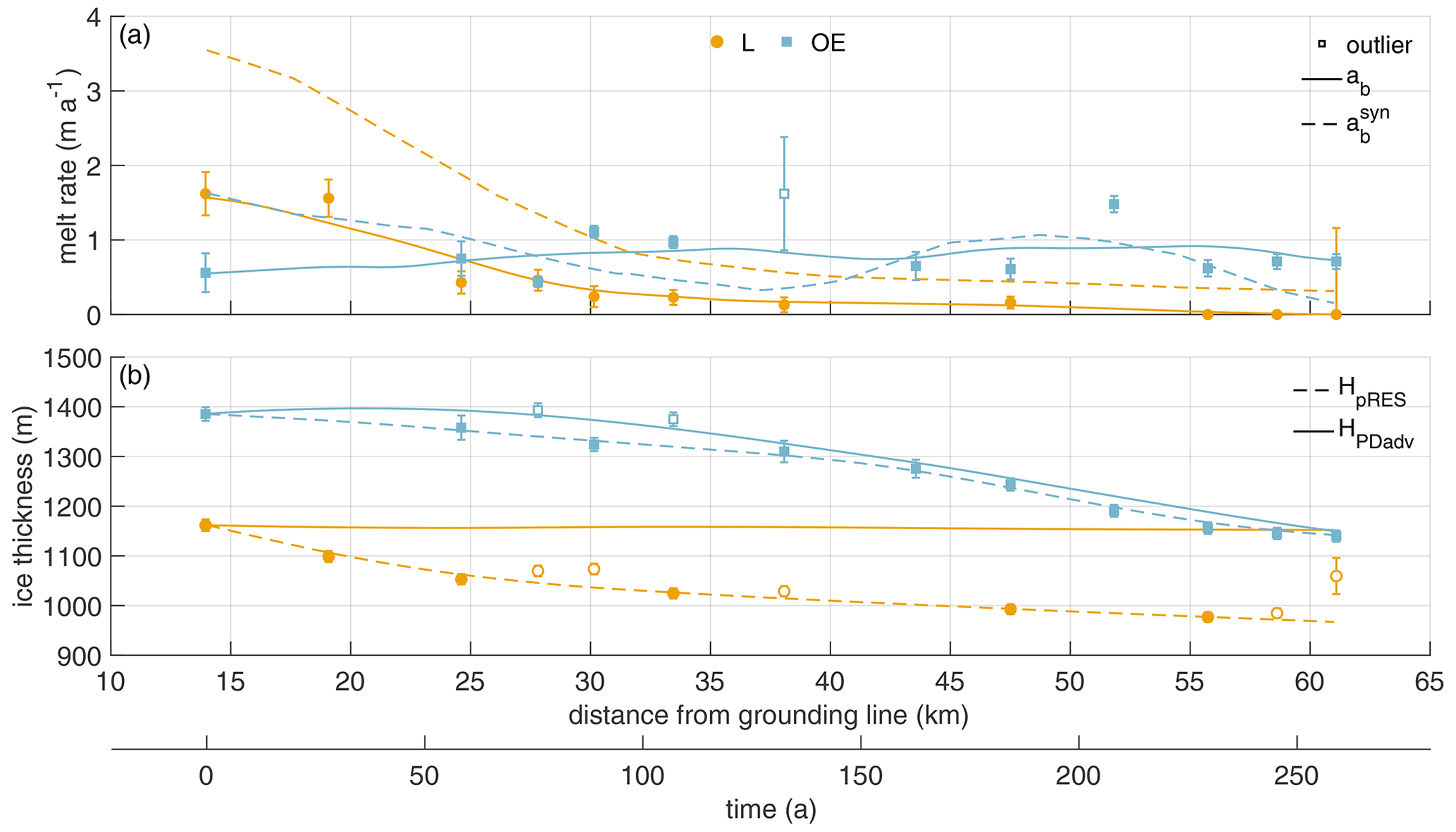
Figure 3(a) Melt rates at locations L (yellow) and OE (blue) are shown by dots (L) and squares (OE). The interpolated melt rates (ab) are shown by solid lines, and synthetic melt rates () that are necessary to reproduce HpRES at L and OE are shown by dashed lines. (b) Ice thicknesses at locations L (yellow) and OE (blue) are shown by dots (L) and squares (OE). The interpolated ice thicknesses (HpRES) are shown by dashed lines, and the advected ice thicknesses under present-day climate conditions (HPDadv) from the observed melt rates at L and OE are shown by solid lines. The two x axes show the distance from the grounding line in kilometers and the duration of ice flow in years from the measurement location furthest upstream. Unconsidered observations were marked as outliers. Error bars mark the uncertainties of the pRES-derived values.
2.3.2 Time series of basal melting
The ApRES time series outside the melt channel reveals an average melt rate of 0.23 m yr−1 (Fig. 4a). A look at the monthly mean melt rates shows increased melt during the summer months (January, February and November, December) in comparison with the winter season. In these months the melt rates show values from more than 0.3 up to 0.62 m yr−1. The spectral analysis of the unfiltered cumulative melt time series shows all main diurnal and semi-diurnal constituents, which is in accordance with the frequencies observed from the GPS station (Fig. A5).
The presence of the tide-induced signal prevents a robust analysis of the basal melt rate as a high-resolution time series. Nevertheless, to investigate the occurrence of non-tidal melt anomalies, we analyzed the time series of ΔH(t) after it was de-tided. The resulting de-tided thinning rate shows several melt anomalies distributed over the entire measurement period (Fig. 4b). These events lasted from a several hours to a few days and melted up to 1.5 cm of ice. In comparison, the annual or seasonal signals have little impact on the thinning rate.
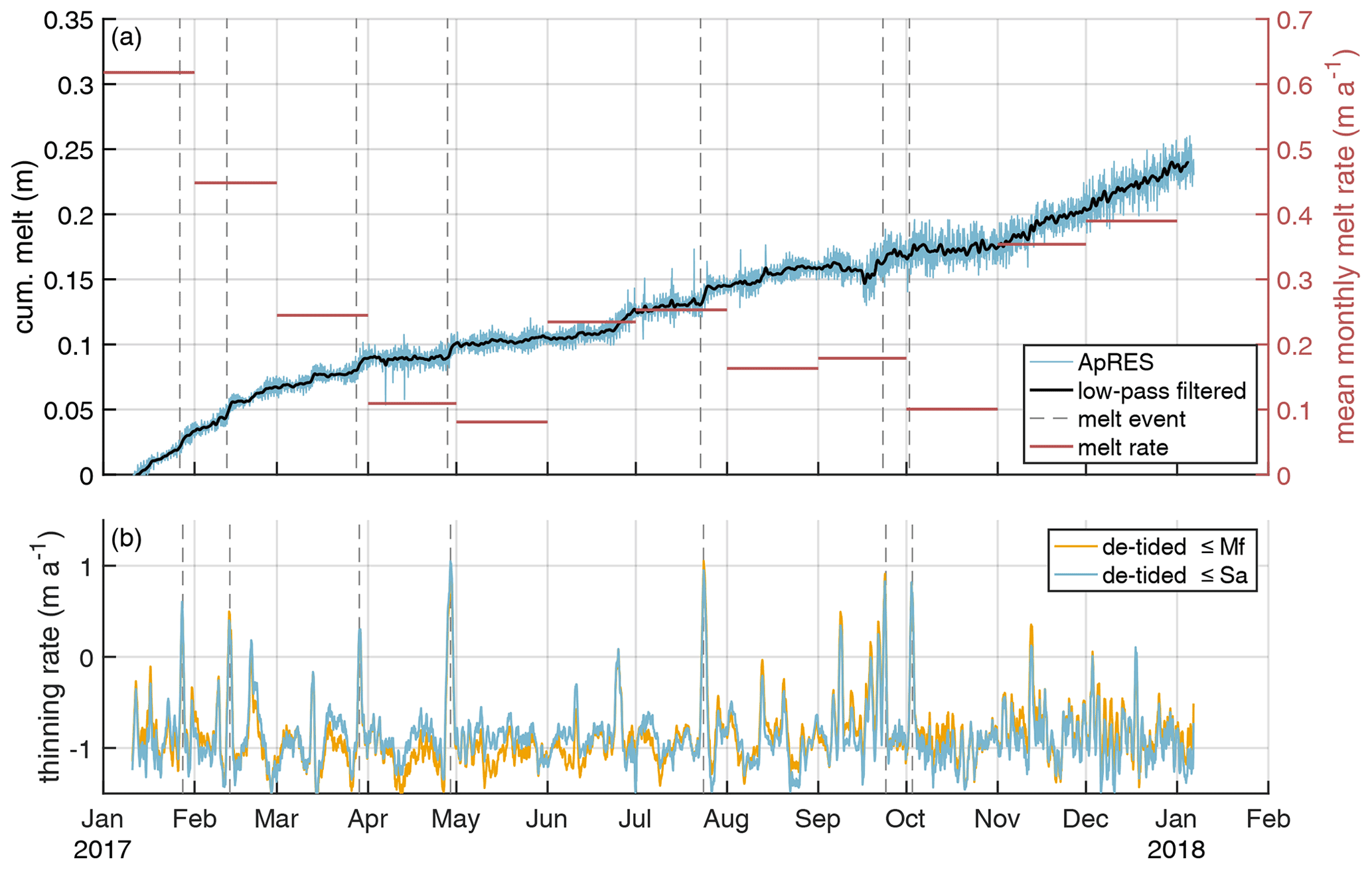
Figure 4Time series of basal melting at the ApRES location outside the channel. (a) Cumulative melt (blue line, left y axis) over the measurement period from 10 January 2017 to 6 January 2018 with low-pass-filtered time series (black line). In September 2017, a malfunction of the ApRES caused a change in the attenuation which resulted in a noisier time series. Monthly mean melt rates are shown by red lines on the right y axis. Due to the inaccuracy in the determination of the strain, the cumulative melt still contains a contribution from strain. (b) Thinning rate after subtracting of the tidal signal up to the fortnightly constituent (yellow line) and up to the solar annual constituent (blue line). The dashed gray lines in panels (a) and (b) mark stronger melt events.
The unfiltered time series of the cumulative melt indicates a tidal signal with amplitudes of ∼1 cm within 12 h around the low-pass-filtered cumulative melt. However, we found evidence that this tidal signal is due to the inaccuracy in the determination of the strain and not a true tidal melt amplitude: we found a clear accordance of the strain in the upper ice column with the tidal signal as recorded by GPS measurements; however, we lack tidal vertical strain in the lower column of the ice due to the noise. As the tidal variation of is by far lower than the observed , either deformations in the upper and lower parts compensate for each other or basal melt/freeze takes this role. We can exclude freezing, as we do not find jumps in the amplitude of the basal return in the ApRES signal (Vaňková et al., 2021) over tidal timescales. Consequently, we infer that strain in the lower half compensates for that in the upper part and there is only a small variation of basal melt on tidal timescales.
As our location is close to two hinge zones, upstream and west of the melt channel, only a full three-dimensional model could shed light on the vertical strain in the lower part of the ice column. This is numerically costly for the required non-linear strain theory and beyond the scope of the project. With melt channels being located (or initiated) in the hinge zone, any kind of ApRES time series performed at thick ice columns might be affected by the unclear strain-depth profile in the lower part of the ice column. This may be overcome by a radar device with higher transmission power, which allows the detection of vertical displacement of layers down to the base. The observed tidal dependency of the vertical strain is consistent with the finding from other ApRES locations at the Filchner–Ronne Ice Shelf by Vaňková et al. (2020). They found the strongest dependency, even of the basal melt rate at some stations, on the semidiurnal (M2) constituent. Besides depth-independent tidal vertical strain, Vaňková et al. (2020) found tidal deformation from elastic bending at ApRES stations located near grounded ice.
For an ice shelf such as the Filchner we expect the principal drivers of basal melting to be the water speed and its temperature above the in situ freezing point (e.g., Holland and Jenkins, 1999). For much of the ice shelf the water speed is dominated by tidal activity (Vaňková et al., 2020), but near the grounding line of SFG we expect the tidal currents to be low, consistent with the evidence from the ApRES thinning rate time series. It is likely that the anomalously high melting events seen in the record result from the passage of eddies, with their associated water speed and temperature anomalies.
To obtain a more profound understanding of the evolution of the channel, we conduct transient simulations and analyze the change in geometry of 2D cross-sections (x, z direction) over time, as well as the simulated strain field. The simulations are forced with the basal melt rates (both interpolated and synthetic) obtained in this study (Fig. 3). We transform distance (y direction) to time in the along-flow direction of the ice shelf (Fig. 1) using present-day velocities. This enables us to study under which conditions the channel is stable or vanishes.
Ideally, we would have observations of ice geometry and basal melt rates from the grounding line onward, but our first cross-section with observations is located 14 km downstream of the grounding line (Fig. 1). The initial elastic response of the grounded ice becoming afloat has faded away. Further elastic contributions to the deformation originate from in situ melt at the base and accumulation at the surface. To best fit the stress state at the first cross-section, we conduct a spin-up.
3.1 Model
The model comprises non-linear strain theory, as there is no justification to expect a priori the simplified, linearized strain description for simulation times longer than 200 years (e.g., Haupt, 2000). We treat the ice as a viscoelastic fluid and solve the system of equations for displacements using the commercial finite-element software COMSOL (Sect. B1; Fig. B1; Christmann et al., 2019). The constitutive relation corresponds to a Maxwell material with an elastic response on short timescales and viscous response on long timescales. For homogeneous, isotropic ice, two elastic material parameters exist (Young's modulus E and Poisson's ratio ν). We conduct all viscoelastic simulations with commonly used values for ice of E=1 GPa and ν=0.325 (Christmann et al., 2019). Another material parameter of the viscoelastic Maxwell material is the viscosity. It controls the viscous flow of ice. We use a constant viscosity of Pa s and discuss the influence of this material parameter later on. This constant viscosity is at the upper limit of the viscosity distribution derived by an inversion for the rheological rate factor in the floating part of the Filchner–Ronne Ice Shelf (Sect. B2 and Fig. B2). This inversion has been conducted using the Ice-sheet and Sea-level System Model (ISSM) (Larour et al., 2012) in the higher-order Blatter–Pattyn approximation (Blatter, 1995; Pattyn, 2003), using BedMachine geometry (Morlighem, 2020; Morlighem et al., 2020), the velocity field of Mouginot et al. (2019b, a), and a temperature field presented in Eisen et al. (2020), based on the geothermal heat flux of Martos et al. (2017). For the assumed material parameters, we obtain a characteristic Maxwell time of τ=153 d by (Haupt, 2000).
The model geometry represents a cross-section through the melt channel (Fig. 5), with the x direction being across channel and resembling the seismic IV profile (Fig. 1) for t=0 year. By assuming plane strain, the shape and the loading do not vary in the along-flow direction (width is sufficiently large). The stress state is independent of the third dimension, the displacement uy in the flow direction is zero and hence all strain components in the direction of the width vanish:
The computational domain is discretized by an unstructured mesh using prisms with a triangular basis involving a refined resolution near the channel. We use the direct MUMPS solver and backward differentiation formula with automatic time step control and quadratic Lagrange polynomials as shape functions for the displacements. The viscous strain is an additional internal variable in the Maxwell model, and we use shape functions of the linear Lagrange type. In some cases, the geometry evolution leads to degraded mesh elements, which requires automated remeshing from time to time.
In this study, the ice density is 910 kg m−3 and the seawater density is 1028 kg m−3. At the upper and lower boundaries, we apply stress boundary conditions: for the ice–ocean interface, a traction boundary condition specifies the water pressure by a Robin-type condition. The ice–atmosphere interface is traction-free. Laterally, we apply displacement boundary conditions. As we take a plane strain approach, we can neglect deformation in the along-flow direction. To obtain realistic lateral boundary conditions, we transform observed vertical strain and, hence, vertical displacements at the location OE in horizontal displacements. First, we assume incompressibility,
and compute the sum of the horizontal strain. We integrate this strain to get a horizontal displacement. Therefore, we assume a homogeneous material, no additional forces in the horizontal direction and a constant ice thickness. The last assumption is not valid inside the channel. However, with a channel of 300 m maximum height over 1 km width, the deviation from outside to inside the channel is small for a computational domain of around 10 km width and an ice thickness around 1300 m. With these assumptions we get a constant strain and integrate this strain to get a horizontal displacement. As we additionally assume plane strain, we can only apply this displacement to the lateral boundary in the across-flow direction. To model the compression and extension of the ice flow through the embayment, we apply the horizontal displacement to each lateral side so that ux becomes
with W the width of the simulated cross-section (Fig. 5). We assume that the horizontal displacements are depth-independent at lateral boundaries, resulting in a compression or elongation perpendicular to the channel (Fig. B3a).
The climate forcing consists of surface mass balance (SMB) and basal melt rate. Technically, both are applied by changing the geometry of the reference configuration with the respective cumulative quantities (Fig. B3b, c). For the SMB, we used multi-year mean RACMO2.3 data (van Wessem et al., 2014) ranging from 0.15 to 0.17 m yr−1 for a density of 910 kg m−3, which we slightly modified to account for the surface depression over the channel: accumulation measurements at the pRES locations indicated higher accumulation in the channel than outside by a factor of roughly 1.5. Thus, we used 50 % higher accumulation rates above the basal channel and a smooth cosine-shaped transition in the x direction. A crucial forcing is of course the basal melt rate. Here we conduct individual experiments that are based on our observed melt rates and their variations. As these data are spatially sparse, we need to interpolate those values in the across-channel (x) direction. We assume a smooth cosine-shaped transition between the observed basal melt rates outside the east of the channel (OE) and inside the channel (L). For melt rates outside the west of the channel, we do not have any observations and assume them to be time-independent. With 10 % lower melt rates than for OE during the spin-up and a smooth cosine-shaped transition between outside the west of the channel and the lowest surface elevation, we get a good agreement of the ice base geometry for outside the west of the channel with seismic IV and V. For the first 20 years after the spin-up, the melt rate outside the east of the channel is higher than outside the west of the channel, whereas afterwards the melt rates in the western part are higher than in the eastern part outside the channel.
As we conduct Lagrangian experiments, we computed the time between the observed measurements through their distance divided by flow velocity. We define t0=0 year at the pRES measurements furthest upstream (Fig. 1) that is also the location of the seismic observation IV by Hofstede et al. (2021a, b). To evaluate our simulations, we compare the simulated surface topography and ice thickness as well as uz(z) with the observed one for the considered time interval of 250 years.

Figure 5The cross-section of the model geometry at the end of the spin-up (t0) of the first experiment shows its corresponding width and ice thickness outside the east of the channel. The boundary conditions of the viscoelastic model are the water pressure pw acting perpendicular to the ice base; the displacement in the flow direction uy, which is zero due to plane strain assumptions; and the time-dependent displacement ux(t) acting in the lateral direction derived by pRES observations. The locations of the pRES station at the lowest point (L) of the channel and outside the east (OE) of the channel are shown at their position on the surface in addition to the SMB (mass increase) and the melt rate ab (mass decrease) at the base of the geometry.
We performed a spin-up to avoid model shocks, introduced by the transient behavior of a Maxwell material, that could be falsely interpreted as the response to geometry changes, for instance, caused by basal melt rates. The main goal here is to have the geometry after spin-up fit reasonably to the geometry measured at the seismic IV line (see Fig. 1) that we denote as time t0. The spin-up covers 75 years, which corresponds to the time from the grounding line to that profile under present-day flow speeds. To this end, we take a constant melt rate equal to the melt rate at t0 and adjust the geometry at the grounding line to match the geometry at t0 of the seismic IV profile reasonably well. After the spin-up, the width W(t0) of the simulated geometry is 10 km. With this procedure the initial elastic deformation at the beginning of the transient simulation vanished and the viscoelastic geometry evolution of the melt channel can be evaluated for different melt scenarios and SMB forcings.
Short-term forces like the time-varying climate forcing as well as the lateral extension or compression demand the usage of a viscoelastic instead of a viscous model to simulate the temporal evolution of the basal channel shown later on. First, we conduct a series of simulations with different material parameters and identify the best match of observed and simulated ice thickness above (L) and outside the east (OE) of the channel. At these two positions, most of the pRES measurements were done, and the distribution of the melt rates gives an adequate basis to force the model. Due to the sparsity of observations at the western side, we apply a forcing in the model based only on melt rates at L and OE.
In the first experiment, we use an interpolation of the observed melt rates as forcing and compare the results with HPDadv (solid lines in Fig. 3). The second experiment aims to derive the best match between simulated and observed geometry. For this experiment, we use synthetic melt rates (dashed lines in Fig. 3a).
3.2 Results and discussion of simulations
3.2.1 First experiment: pRES-derived melt rate
The spin-up for this experiment starts with a manually adjusted geometry (including the channel at the base) at years to fit seismic IV profile at t0. We applied a constant melt rate of 1.5 m yr−1 at L and 0.5 m yr−1 at OE. This forcing enlarges the melt channel during the spin-up as the ice thickness OE increases due to the prescribed displacement representing compression caused by the lateral boundaries moving towards the center of the channel. The general shape of the base matches the seismic profile IV reasonably well (Fig. 1 and Fig. B4). After the spin-up, we force the base with ab (solid line in Fig. 3a).
The results of this experiment are displayed in Fig. 6. For both locations, L and OE, the simulated geometry and observed geometry differ significantly. The simulated ice thickness above the channel declines by 21 m in 250 years, while the observed thickness is 191 m thinner. Outside the channel, the simulated trend shows thinning. This thinning begins after 50 years, whereas we find continuous thinning in the observations. This delayed onset of thinning is also represented in the simulated surface topography. Most notable is the match between simulated Hsim and advected HPDadv ice thickness under present-day climate conditions at the center of the channel (L). At the same time, the mismatch to HpRES confirms that present-day melt rates would not lead to the observed channel evolution over 250 years.
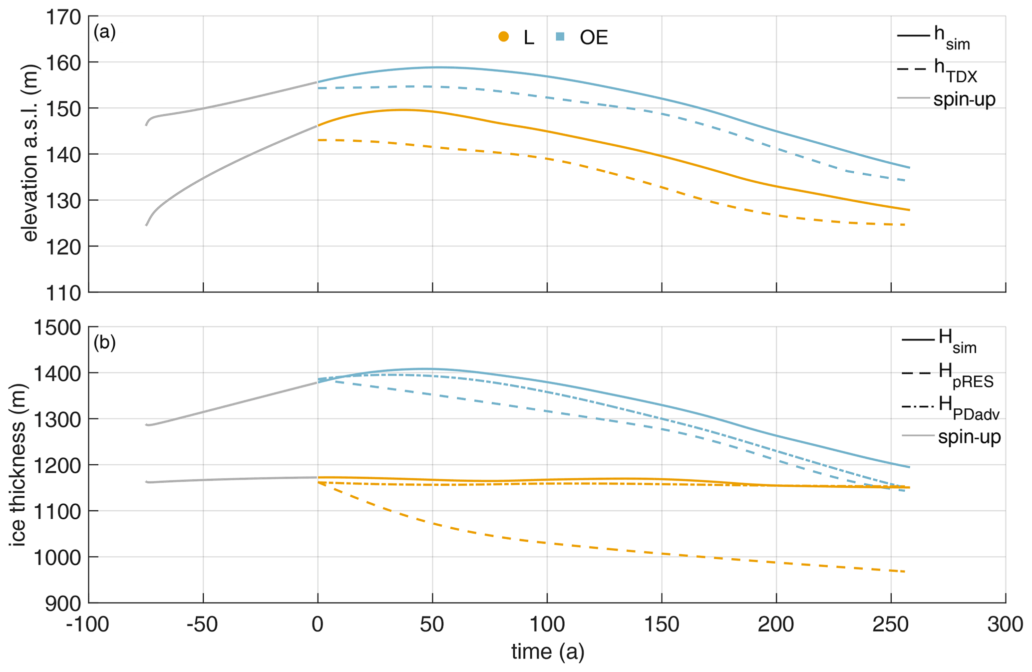
Figure 6First experiment: simulated surface elevation (a) and ice thickness (b) using the pRES-derived melt rate. Colors denote quantities above the channel (yellow) and outside the channel (blue). (a) Simulated surface elevation hsim (solid lines) and observed hTDX (dashed lines). (b) Simulated ice thickness Hsim (solid lines), under present-day climate conditions advected HPDadv (dashed-dotted lines) and observed HpRES (dashed lines). Gray lines represent the spin-up.
3.2.2 Second experiment: synthetic melt rate
The spin-up for the second experiment starts with a different geometry than the first experiment as the basal melt rate is different. However, it has also been manually adjusted at years to fit seismic IV profile at t0. In the second simulation experiment, we force the base with the synthetic melt rate (Fig. 3a) that is larger inside the channel than the observed melt rate. Again, the melt rate has been kept constant over the spin-up with . The synthetic melt rate leads to a cumulative melt after 250 years of 290 m (Fig. B3a), with 184 m more ice melted at L than in the first experiment, and, hence, the initial geometry has to be different to the first experiment; hence, we conduct an own spin-up simulation for the second experiment.
The modeled geometry of this experiment is presented in Fig. 7. The simulated ice thickness at L is in very good agreement with HpRES. There is some mismatch at OE, but the simulated trend of thinning is synchronous to the observations. After 250 years the deviation from the observed ice thickness at OE reaches +53 m. The simulated base for the second experiment shows a persistent basal channel (Fig. B5). The mismatch of the surface elevation at L and OE reverses over time: while the simulated surface topography at OE is at first too low, it is too high in the second half of the transient simulation (Fig. 7). However, the trends of the observed hTDX and simulated hsim elevation behave similarly. While ice thickness is in good agreement, surface elevation above the channel is overestimated by 4 m at the end of the spin-up. After 57 years, it turns from an overestimation to an underestimation that results in an 8 m lower hsim than the observed hTDX after 250 years. To understand if the ice is in hydrostatic equilibrium, we compute the freeboard at the position L for an ice density of 910 kg m−3. The surface elevation is 133 m at t0 and decreases to 112 m after 250 years. Although hTDX is larger than this, the ice is approaching flotation in the downstream direction. One could take another approach and estimate the mean density under the assumption of buoyancy equilibrium: at t0 this corresponds to 901 kg m−3, and after 250 years this corresponds to 896 kg m−3. As more ice is melted from below and with higher snow accumulation at L, the density decreases, which is to be expected.
After 250 years, the simulated freeboard at L is 1 m higher than the surface elevation of 138 m inferred by buoyancy equilibrium using an ice density of 910 kg m−3, and at OE the discrepancy is 3 m. Overall, we see convergence to equilibrium state at OE and the simulated surface elevation at L. At the end of the simulation, only hTDX above the channel does not reach buoyancy equilibrium, which leads to the justifiable assumption that the mean ice density at L is lower than OE.
At the position of the furthest upstream pRES observations, we know from interferometry shown in Hofstede et al. (2021a) that the location is still in the hinge zone. The assumption of buoyant equilibrium is therefore likely to be flawed. At the end of the simulation, the geometry should be close to buoyancy equilibrium despite melting and a 50 % higher SMB at L than OE. Hence, simulations carried out using a higher SMB within the channel would result in better agreement with the observed values of hTDX.
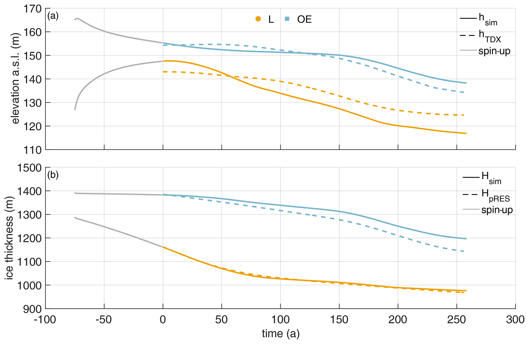
Figure 7Second experiment: simulated surface elevation (a) and ice thickness (b) using the synthetic melt rate. Colors denote quantities above the channel (yellow) and outside the channel (blue). (a) Simulated surface elevation hsim (solid lines) and observed hTDX (dashed lines). (b) Simulated ice thickness Hsim (solid lines) and observed HpRES (dashed lines). Gray lines represent the spin-up.
Next, we consider the variation of the vertical displacement with depth. The results are presented in Fig. 8. For this purpose, we calculated the cumulative vertical displacement in 1 year. For comparability, the vertical displacements due to accumulation and snow compaction were removed from the observed distributions. Most notably, we move from a vertically extensive regime to a compressive regime with increasing distance from the grounding line. Given the complexity of the problem, the simulations show a reasonable agreement with the observations. The best match is reached at OE, which is not that surprising. The generally good agreement of the simulated displacements outside the channel comes from tuning ux at the lateral boundary to match uz from the pRES measurements at OE. A schematic illustration of first principal strains and their directions shows a closure of the channel for lateral compression and simultaneously a thickening of the ice shelf that is larger inside the channel than outside (Fig. B6). For lateral extension, we conversely get a thinning of the ice shelf that is smaller inside the channel than outside. Both simulated and observed vertical displacement distributions show that the strain decreases from L to OE (Fig. 8). The only exception here is t=57 years, where the vertical strain at SE is larger than the one at L, in the observations. While at 0 and 26 years the deviation of the simulated displacements between L and OE is small, it increases afterwards. From 105 years, the simulated vertical displacements agree very well with those of the pRES measurements, where a displacement distribution was derivable at L and OE. The same comparison for the first experiment (Fig. B7) shows similar results, with significantly less pronounced differences between L and OE. Hence, the mismatch to the observed vertical displacements for this experiment using the measured melt rates is higher than for the second experiment with the synthetic melt rates.

Figure 8Second experiment: comparison of displacements (uz) derived from observations (dots) and the simulations (lines). The different panels show the displacement for Δt=1 year allocated to the simulation time (upper right corner). The numbers in the lower right corners give horizontal displacement ux derived from εzz of the pRES measurements outside the channel (OE), with positive values representing compression and negative values extension.
As the last point of this second experiment, we consider the influence of the viscosity on the evolution of the melt channel (Fig. B8). To reach the ice thickness of seismic IV, the simulation applying the smallest viscosity needs a higher initial channel at the beginning of the spin-up (Sect. B3). The channel thickness of the pRES measurement is modeled best using a viscosity of 5×10¹⁵ Pa s. A 2-times-higher viscosity leads to a geometry where the ice is 42 m thinner in the center of the channel after 250 years, while a 5-times-lower viscosity results in 116 m thicker ice above the channel due to more viscous flow into the channel. The simulated ice thickness OE is similar for all three different viscosities. The distributions of vertical displacement with depth illustrate that the difference between L and OE is larger for smaller viscosity values (Fig. B9). Often the viscosity of 5×10¹⁵ Pa s fits quite well to obtain the observations by the simulation, but for some a slightly (Fig. B9a) or a considerably lower viscosity (Fig. B9c) would be needed.
We also conducted simulations to test with extreme high melt rates along the steep slopes at the flanks, which did not lead to a reasonable evolution of geometry of the channel, and they are therefore not presented here.
First we aim to compare our findings with other measurements inside a melt channel, which are unfortunately still very sparse, and we want to emphasize here that there is a strong need for more of this type of observation in the future. We find that melt rates inside the channel are in general rather modest, <2 m yr−1. Values retrieved at a channel 1.7 km from the grounding line at the inflow of the Mercer and Whillans ice streams into the Ross Ice Shelf were 22.2 m yr−1 (Marsh et al., 2016). These values dropped to below 4 m yr−1 over a distance of 10 km and reached 2.5 m yr−1 after 40 km. We also find that the melt rates decrease by a factor of 5 in the center of the channel over a distance of 11 km; however, this takes place between 14 and 25 km downstream of the grounding line. At the Ross Ice Shelf, the ratio between the melt rates inside the channel and 1 km outside it is about 27, whereas we find only a factor of 3, with the distance between L and OE being 1.8 km.
Zeising et al. (2022b) presented pRES-derived basal melt rates downstream of our study area. Roughly 40 km downstream of the northernmost cross-section (∼200 years of ice flow), these measurements show that the channel still exists, but with a small height of ∼16 m. Inside the channel, Zeising et al. (2022b) determined a melt rate ∼0.20 m yr−1 lower than outside. The larger melt rates outside the channel compared to inside are in agreement with the finding of our study. In general, the channel height declines, so the channel fades out. The channel diminishes because melt rates inside the channel fall below those outside the channel. The trend in vertical strain has only a minor contribution to this evolution. We thus do not find any evidence that such channels are a cause for instabilities of ice shelves as suggested by Dow et al. (2018).
One of the main findings of our study is that the present geometry can only be formed with considerable higher melt rates in the past (see Fig. 3). This finding is based on the assumption that the strain rates were in the past similar to the present day and that melt on both flanks of the channel is similar. This is justified, as significant changes in strain would require a change in the system that would cause other characteristics to change, like the main flow direction, for which we do not find any indication. However, in our setting, we are in a compressive regime. A similar assumption may not be possible at other locations.
The pRES melt rate observations covered only 1 year. As the ocean conditions within the sub-ice shelf cavity are known to respond to the ocean forcing from the ice front (e.g., Nicholls, 1997), we would expected them to be subject to significant interannual variability. Underlying any interannual variability, a long-term reduction in basal melt rates would be the expected response to a reduction in production of dense shelf waters north of the ice front, resulting from a reduction in sea ice formation (Nicholls, 1997), which in turn results from a reduction in the southerly winds that blow freshly produced sea ice to the north.
A decrease in northward motion of sea ice has been observed in the satellite record (e.g., Holland and Kwok, 2012), but no observation of sea ice trends over 250 years is available to our knowledge. The modeling experiments by Naughten et al. (2021) also find decreasing ice shelf basal melt rates. This reduction is therefore consistent with higher basal melt rates in the past. However, our model results suggest that the mismatch between the past melt rates needed to explain the channel geometry and the present-day observed melt rates applies only to the channel and not to the ambient ice. This could be explained by historically higher levels of subglacial outflow at the grounding line or anomalously low levels during the observation period. Subglacial outflow contributes to the buoyant flow up the basal slope and therefore the shear-induced turbulence that raises warm water from deeper in the water column towards the ice base. Variations in the subglacial outflow could be caused by variations in subglacial storage, as Smith et al. (2009) found an active subglacial lake at the transition between Academy Glacier and SFG, and Humbert et al. (2018) also suggest the presence of a subglacial lake in the upstream area of SFG.
Hofstede et al. (2021a) showed that the subglacial channel appears 7 km upstream of the grounding line, increasing its height to 280 m at the grounding line. The location of the channel corresponds with increased subglacial flux found by Humbert et al. (2018) using a simple routing scheme. Once this topographic feature reaches the ocean, it serves to focus the buoyant plume and enhance shear-driven vertical mixing, bringing heat and salt to the ice base and leading to higher basal melt rates.
However, with increasing distance along the channel, the basal gradient, and therefore the speed of the buoyant flow, is reduced, which also reduces the entrainment of warm water from beneath. Coupled with the pressure-induced increase in the freezing point with decreasing depth, this leads to a gradual reduction of the melt rate in the channel. From Fig. 2a, the melt rate in the channel reduces below that of the ambient ice base by about 30 km distance from the grounding line, suggesting that the effect of focused meltwater outflow thereafter is to suppress the channel.
The cause of the strong melt anomalies identified in the ApRES measurements remains unclear as no direct ocean observation exists near SFG. However, the timescale of the events is consistent with the passage of warm cored eddies. Such features have been observed in the ocean cavity beneath the neighboring Ronne Ice Shelf (Nicholls, 2018).
The channel height is found to increase until 30–35 km downstream of the grounding line. Further downstream, the channel begins to close. Our modeling results show that less viscous ice (1×10¹⁵ Pa s) would tend to shut the channel faster than the rate we observe (Fig. B8). For the best match between observed and modeled geometry, we need viscosities around 5×10¹⁵ Pa s to prevent closure by deformation (Fig. 7). This viscosity value is also supported by an inversion of ice rheology to fit observed surface velocities in the melt channel region (Sect. B2). With a viscosity of 5×10¹⁵ Pa s, we can use a viscoelastic model to simulate the channel evolution in both experiments to match the observations: (i) pRES-derived melt rates result in an ice thickness fitting the present-day advected ice thickness HPDadv (Fig. 6), and (ii) synthetic melt rates lead to the observed ice thickness HpRES (Fig. 7). The channel vanishes for the pRES-derived melt rates as those are unable to maintain the channel geometry open against viscoelastic deformation (Fig. B4). Based on the higher synthetic melt rates, the simulated basal channel remains open, and we get a similar basal shape to that found by the seismic measurements (Fig. B5). However, if we would want to match the observed basal geometry at seismic profile V more precisely, we would have to spatially vary the basal melt rate in the across-flow direction, enlarge the transition between L and OE, and thus extend the channel to the eastern side.
To evaluate the importance of using a viscoelastic and not a purely viscous material law, we compute the logarithmic Hencky strain (Sect. B4). With this strain measure, an additive decomposition of the strain into an elastic and viscous part is possible. After the spin-up, the elastic strain components in the across-flow and thickness direction are on the order of 0.1 % and 1 order of magnitude larger than the shear component (Fig. B10). Christmann et al. (2021) derived similar magnitudes in the viscoelastic simulation of 79∘ North Glacier considering linearized strains. The magnitude of elastic strain in the across-flow direction is caused by the lateral compression and varies slightly to higher values around the channel due to the geometry of the channel. However, the highest elastic strain values are reached outside the channel and decrease with time (Fig. B11). It is likely that the elastic deformation slightly increases especially inside the channel if the lateral compression changes into tension or vice versa. In the thickness direction, the elastic strain is decreasing towards the channel (Fig. B10b). This causes the difference in geometry change, due to different values of the viscosity, to be larger inside the channel rather than outside (Fig. B8). The simulated geometry change is mainly due to the elastic response to thinning by basal melt and ice accumulation. Any purely viscous simulation would overrate the deformation in the vertical direction as the elastic strain has the opposite sign as the viscous one (Fig. B12d–f). Higher melt rates were needed to compensate for this. Wearing et al. (2021) presents a full Stokes simulation of a comparable melt channel and indeed needs higher melt rates to keep the channel open. The relative amount of elastic strain shows values up to 8 % of the total strain for high lateral compression or extension and is hence not negligible (Fig. B10). It is important to keep this result in mind for future inverse modeling of melt rates in melt channels.
We find a difference (−4 to 8 m) between simulated and observed surface elevation at L (Fig. 7). The elevation difference is most likely caused by the constant density that we used for the simulations, as the ice thickness matches well. For the thinner ice above the channel, this could be achieved by an ice density decreasing from outside to inside and from upstream to downstream in the channel. However, one has to keep in mind that the accuracy of the surface elevation product is only 5 m, so the differences in surface elevation may not be significant.
In general, we benefited highly from having measurements of vertical strain available. This opens new possibilities to identify weaknesses in the modeling, such as limited knowledge on lateral boundary conditions and rheological parameters, and it gave us useful insight into the spatial variation of the vertical strain across such a topographic feature (Figs. 8 and B7). Although the pRES surveys only about half the ice thickness, the slope of uz(z) in the upper half is distinct for the positions L, SE and OE; greatly varies with distance from the grounding line; and is also influenced by the embayment of the ice shelf. Simulated uz at L starts to match well with observations after about 100 years, which could result from the first few cross-sections still being influenced by the hinge zone (Fig. 8). Tidal bending was not taken into account here, due to the 2D setting. This could in the future be investigated if repeated pRES measurements were to be conducted up to the grounding line covering the entire hinge zone, in which case it would also be extremely advantageous to obtain basal melt rates at tidal timescales. In addition, in the future, melt rates should be obtained on both flanks of the melt channel, as well as having an coverage of the melt channel with airborne surveys to have detailed knowledge of the entire 3D geometry.
Our study demonstrates that viscoelastic simulations can be a useful but complex tool to analyze melt channel evolution. In an inverse approach, viscoelastic models could also give more insights into basal melt rates of channel systems of ice shelves in general, given that satellite-borne surface elevation is available in high resolution. However, the fact that large deformations require non-linear strain theory will make this a challenging endeavor. As changes in basal melt rates will inevitably lead to surface elevation changes of channel systems, systematic monitoring of the surface topography from space can serve as an early warning system and trigger further in situ observation similar to this study.
We find basal melt rates in a melt channel and its surroundings on Filchner Ice Shelf to be up to 2 m yr−1. Basal melt rates inside the channel drop with distance downflow, even turning into freezing 55 km downstream of the grounding line. Close to the grounding line, melt rates are larger inside the channel than outside, while further downstream this relationship reverses. Along flow, the channel height decreases from a maximum of 330 m to below 100 m. The channel diminishes because the reduced melt rate is unable to maintain the channel geometry against viscoelastic deformation. Analysis of the predicted ice thickness from advection of present-day thickness with present-day melt rates revealed large differences compared to the observed ice thickness above the channel, which indicates that melt rates have been about twice as large in the last 250 years. The viscoelastic simulation confirms this statement and indicates that basal melt channels need high basal melt rates and relatively cold ice to persist. The deformation of the basal melt channel is mainly driven by the elastic response to the basal melt rate. The observed and simulated evolution of this melt channel demonstrates that melt channels of this kind (where melt rates inside the channel are small and turn to freezing downstream) are not a destabilizing element of ice shelves. The ApRES time series showed brief melt anomalies distributed over the entire measurement period and slightly increased melt rates in summer.
A1 Basal reflections and the influence of off-nadir returns
The identification of the basal reflections in both measurements, the first and the repeat measurement, is important in order to determine the change in ice thickness and thus the basal melt rate. Due to a high contrast in relative permittivity, the ice–ocean interface is a particularly strong reflector. Accordingly, the reflection at the ice base in the echogram is characterized by a sharp increase in amplitude. After identifying the first basal reflection in both measurements, the vertical displacement can be determined by means of a cross-correlation of the basal segment, provided that the shape of the basal reflector has not changed significantly. However, this was not the case at 5 of the 44 stations in our study area. At these, the basal return had changed significantly and thus prevented an unequivocal match. We therefore excluded these stations from the melt rate analysis. At all other stations, the reflection had changed only slightly, so that the vertical displacement could be reliably determined. Figure A2 shows three examples (OE, SE and L) from a cross-section 48 km downstream of the grounding line. In all of these measurements, a strong increase in amplitude was found between 992 m (L) and 1244 m (OE), which represents the first onset of the basal reflections. While the shape of the basal return changed only slightly, there was a change in amplitude, which is lower in the repeat measurement, especially in Fig. A2e and f. One potential reason for this was different measurement settings that influenced the amplification of the signal, but imprecise alignment of the transmitting and receiving antennas can also be responsible for this.
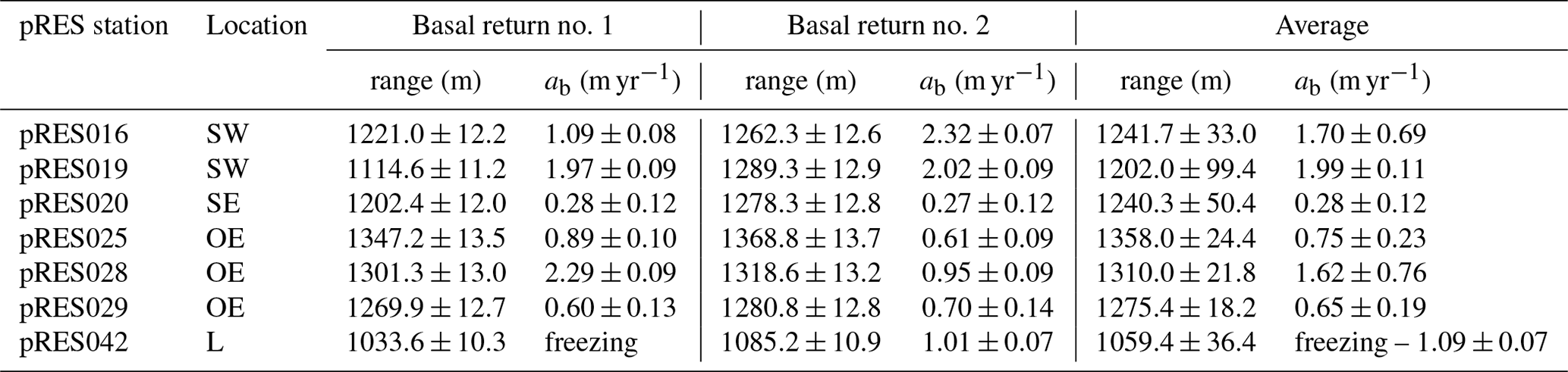
However, at 7 of the 44 stations more than one strong and clear defined basal reflection was found, raising the question of which is the nadir and which is the off-nadir reflection. The reason for this is that a steep base, such as on the flanks of the channel, creates strong off-nadir reflections. Depending on the basal gradient, this off-nadir reflection may also arrive before the nadir reflection. As pRES data represent point measurements, they cannot be used to constrain the local shape of the ice base, and thus distinguishing nadir from off-nadir returns is difficult. One possible indicator of the nadir reflection can be the reflection amplitude, since the antenna radiates most of its energy in the nadir direction. However, in certain basal geometries off-nadir reflections can still be stronger than the nadir reflection, even accounting for the antenna beam pattern. Figure A3 shows two examples of stations with off-nadir reflections. In the measurements at the pRES029 station (OE; Fig. A3a, b), the basal reflection with the largest amplitude appeared with a range 11 m greater than the first basal reflection. This could be an indication that the first basal reflection is an off-nadir return. The analysis of the vertical displacement of both basal reflections shows a deviation of 0.13 m. The second example from station pRES019 (SW; Fig. A3c–e) shows two basal reflections of approximately equal strength, separated by about 175 m. At this station, the deviation of the vertical displacement of both basal returns was only 0.01 m. Which of these reflections is the nadir and which is the off-nadir reflection cannot be reliably determined from the pRES measurement. Only by analyzing the basal geometry, e.g., by airborne radar or seismic profiles, can the reflection be assigned to its place of origin by determining the basal distances from the measurement location. However, since seismic profiles are only available in the vicinity of two cross-sections, this method cannot be used for all stations. Thus, we calculated the displacement of the second and strongest basal return of those seven stations where more than one strong basal return occurred. The melt rates derived from the first and the second basal return are shown in Table A1. While at three sites the difference in melt rate is below 0.1 m yr−1, at others, the melt rate difference exceeds 1 m yr−1. Since we cannot distinguish between nadir and off-nadir solely from our pRES measurements, we have averaged the two derived melt rates and taken into account the difference in the error. However, at station pRES042 (L) we found basal freezing by analyzing the first basal return but derived a melt rate of 1.09±0.07 m yr−1 from the second, stronger basal return. We designate this location as a basal freezing station and state the range of melt rate as an error.
A2 Additional table

A3 Additional figures
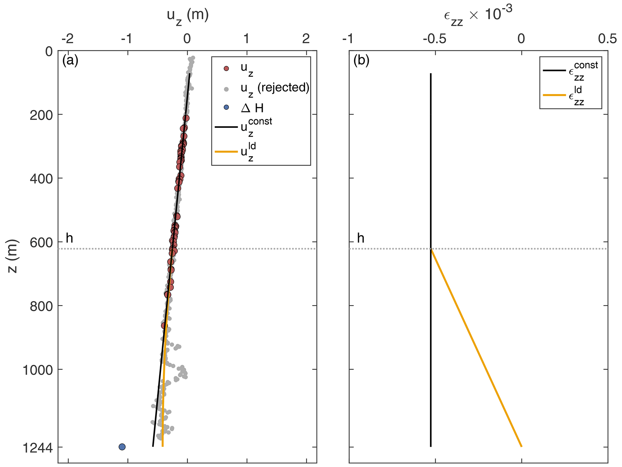
Figure A1Strain analysis of a pRES measurement at location OE (pRES30; 48 km from grounding line). (a) Derived vertical displacements uz for Δt=1 year of the ice base (ΔH; blue dot) and internal layers (red and gray dots). Displacements used for the linear regression (black line) are colored in red, and rejected displacements are shown in gray. The second model with a linear decreases (ld) from depth h (dotted line) to zero at the ice base is shown in orange. (b) Vertical strain for Δt=1 year of both models whose displacement is shown in panel (a).
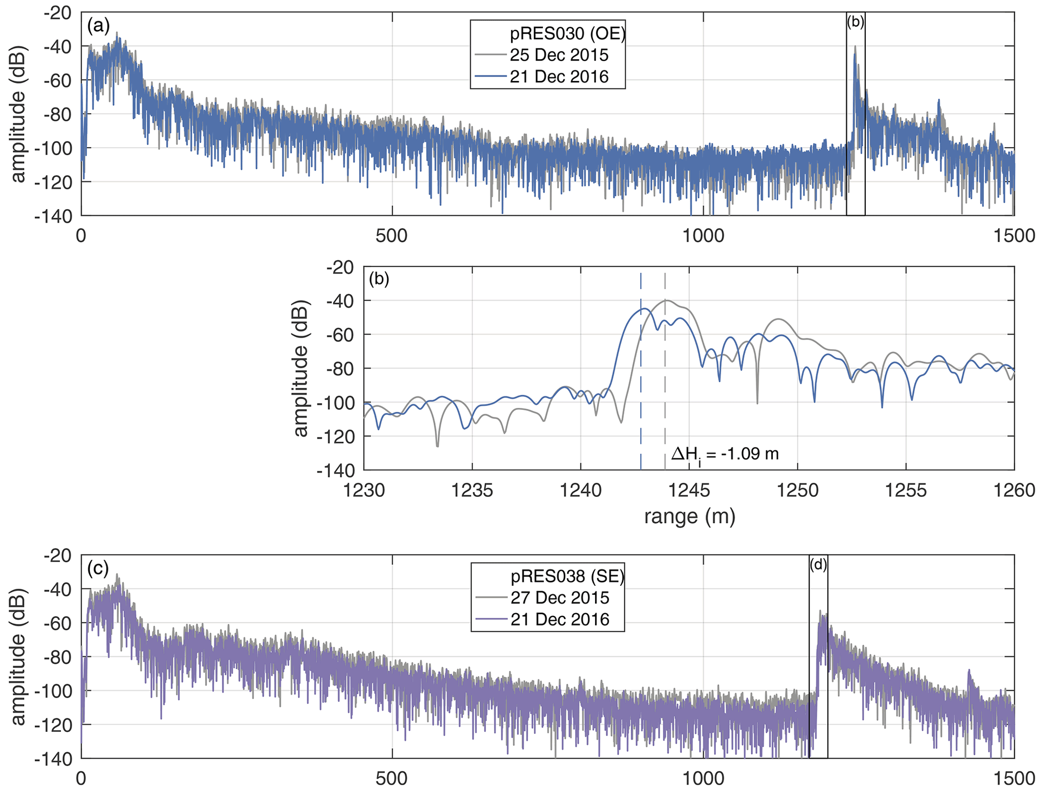
Figure A2Amplitude profiles of first (gray line) and repeated pRES measurements at locations OE (a, b; blue), SE (c, d; purple) and L (e, f; red), all at the cross-section with a distance of 48 km from the grounding line. (b, d, f) Enlarged basal section, visualized by black boxes in panels (a), (c) and (e). Vertical dashed lines mark the ice thickness and ΔHi the change in ice thickness between both visits.
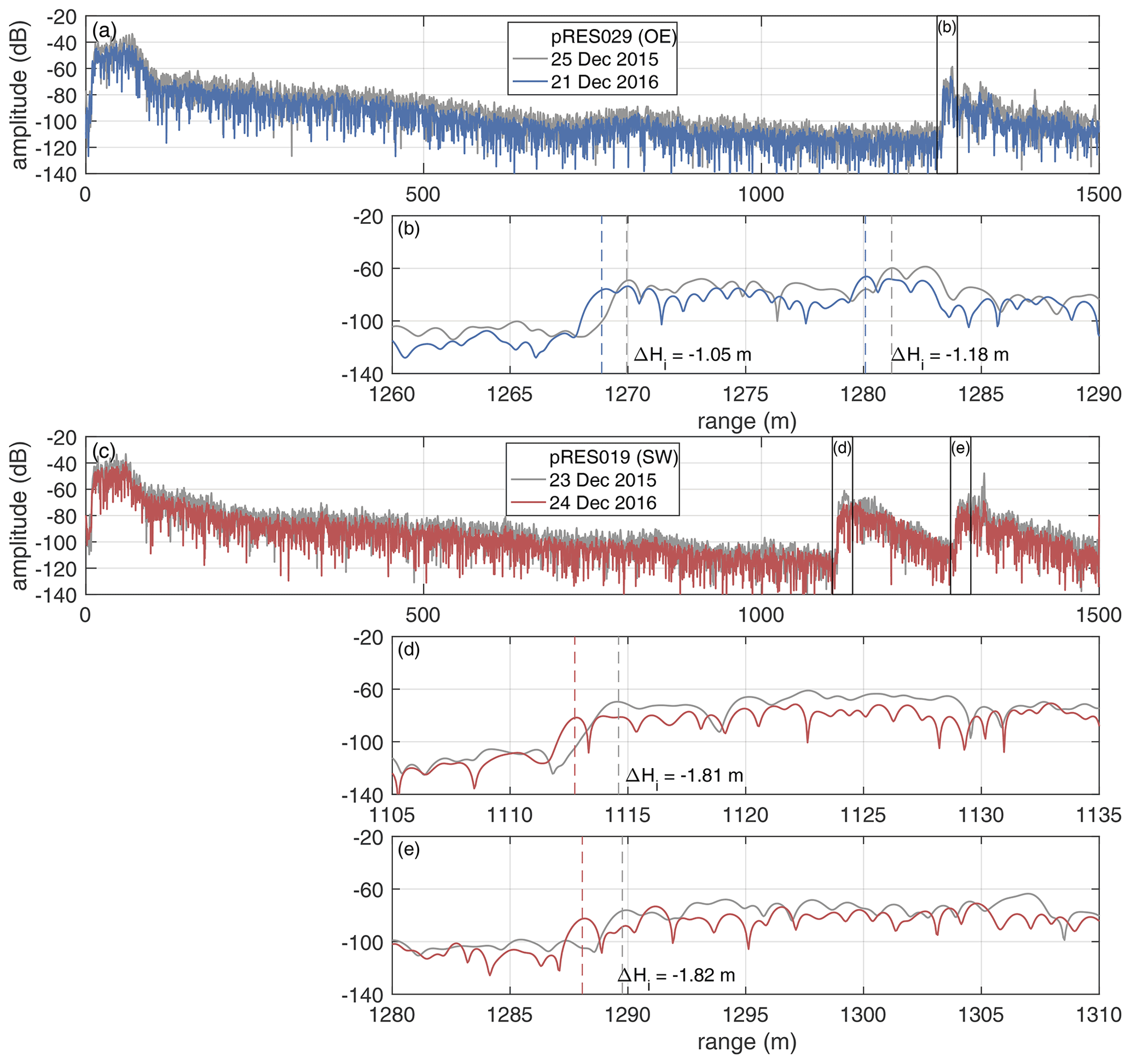
Figure A3Amplitude profiles of two measurements indicating off-nadir basal reflections. (a, b) First (gray line) and repeated pRES measurement (blue) at location OE at the cross-section with a distance of 43 km from the grounding line. (b) Enlarged basal section, visualized by black boxes in panel (a). Vertical dashed lines mark the ice thickness and ΔHi the change in ice thickness between both visits for the first and second strong increase in amplitude. (c–e) First (gray line) and repeated pRES measurement (red) at location SW at the cross-section with a distance of 28 km from the grounding line. (d, e) Enlarged basal sections, visualized by black boxes in panel (c). Vertical dashed lines mark the ice thickness and ΔHi the change in ice thickness between both visits for the first and second strong increase in amplitude.
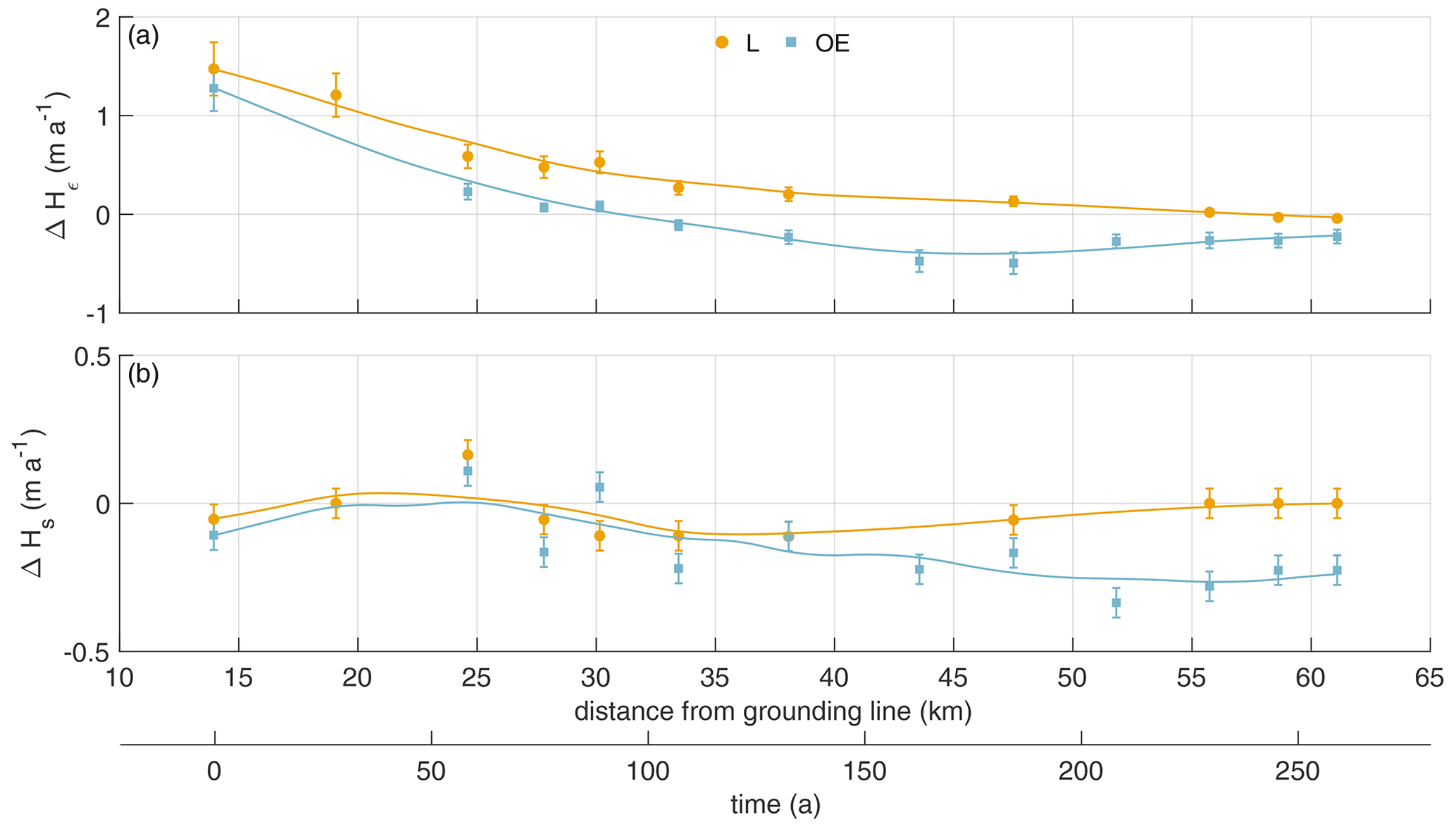
Figure A4Distribution of pRES-derived (a) change in ice thickness due to strain and (b) ice thickness change due to surface process (firn compaction and accumulation) above the channel (yellow dots) and outside the east of the channel (blue squares). The solid lines represent a smoothed fit. Error bars mark the uncertainties of the pRES-derived values.

Figure A5(a) Surface elevation recorded by the GPS station from the end of December 2015 to early April 2016. (b) Linear de-trended cumulative melt (ΔHb) from ApRES observations between January 2017 and January 2018. (c) Frequency spectrum from data shown in panels (a) and (b). Vertical gray dashed lines mark the constituents with half-day periods (N2=12.66 h, M2=12.42 h, S2=12.00 h, K2=11.97 h), daily periods (Q1=26.87 h, O1=25.82 h, P1=24.07 h, K1= 23.93 h) and fortnightly period (MSf =14.76 d). Notice that due to a shorter measuring period of the GPS, the resolution in frequency space is lower than that of the ApRES.
B1 Viscoelastic model for nonlinear strains
This section presents the basic equations for a viscoelastic Maxwell model applicable for finite strains. To consider finite deformations, we need to distinguish different configurations (Fig. B1). The reference configuration (stresses and strains denoted by the subscript 0) includes all positions X of material points in an initially undeformed domain. The displacement vector field relates the particle position vector X in the reference configuration to its spatial position x in the current configuration depending on the external load and the time passed (Fig. B1). To formulate differential equations for finite viscoelasticity, we focus on the system of equations with respect to the reference configuration, which is frequently applied in solid mechanics Haupt (2000).
In the reference configuration, the quasi-static momentum balance reads
with Div(⋅) the divergence with respect to the reference configuration. The tensor is the first Piola–Kirchhoff stress containing the Jacobian determinant J=det(F), the Cauchy stress σ of the current configuration and the transposed inverse of the deformation gradient
characterizing the material gradient of motion in which I is the second-order identity tensor. The volume force accounts for the gravitational force in the thickness direction using the ice density ρice=910 kg m−3, the acceleration due to gravity g and the upward-pointing unit vector . The formulation for finite viscoelasticity uses the conceptual multiplicative decomposition of the deformation gradient
into rate-independent elastic (e) and rate-dependent viscous (v) parts (Lee, 1969). All material equations are formulated in the intermediate configuration (stresses and strains denoted by ) as an additive decomposition of the strain (similar to linearized strain; Christmann et al., 2019) is feasible in the intermediate configuration
The elastic strain is given by and the viscous strain by . For a viscoelastic Maxwell model, the viscous stress is equal to the elastic stress in the intermediate configuration. If we assume a Saint Venant–Kirchhoff material for the elastic material, we get
with the viscosity η, the first Lamé constant and the deviatoric part of the elastic strain . The viscous strain rate is defined using the objective lower Oldroyd rate , with the viscous deformation rate and the time derivative denoted by the superimposed dot.
For the viscoelastic simulation, we have to formulate all equations and boundary conditions in the same configuration; here, we choose the reference configuration. Beside solving the momentum balance (Eq. B1), we solve the material law:
with the symmetric second Piola–Kirchhoff stress , the second Lamé constant and the right Cauchy–Green tensor C=FTF. For a viscoelastic Maxwell material, we have to compute elastic or viscous deformations through an internal variable in the reference configuration. The evolution equation for the internal variable reads
At last, we have to define the boundary conditions in the reference configuration. Dirichlet conditions are the same in reference and current configuration, while traction boundary conditions change due to adjusting normal vectors for the different configurations. To model compression and extension, the horizontal displacements acting on the lateral boundaries are computed out of the observed strain at the position OE:
with ux the displacement component in the across-flow direction (Eq. 12, Fig. 5). The upper surface is traction-free, and the base perceives the depth-increasing water pressure of the current configuration,
in the normal direction with sea water density ρsw=1028 kg m−3 and uz the displacement component in the thickness direction. Hence, we have to compute the water pressure in the reference configuration,
with the pressure P0 and the normal vector N in the reference configuration as well as the pressure p and the normal vector n in the current configuration. Additionally, we deform the geometry by temporally and spatially variable fields of basal melt subtracted at the lower boundary and SMB added to the upper boundary.
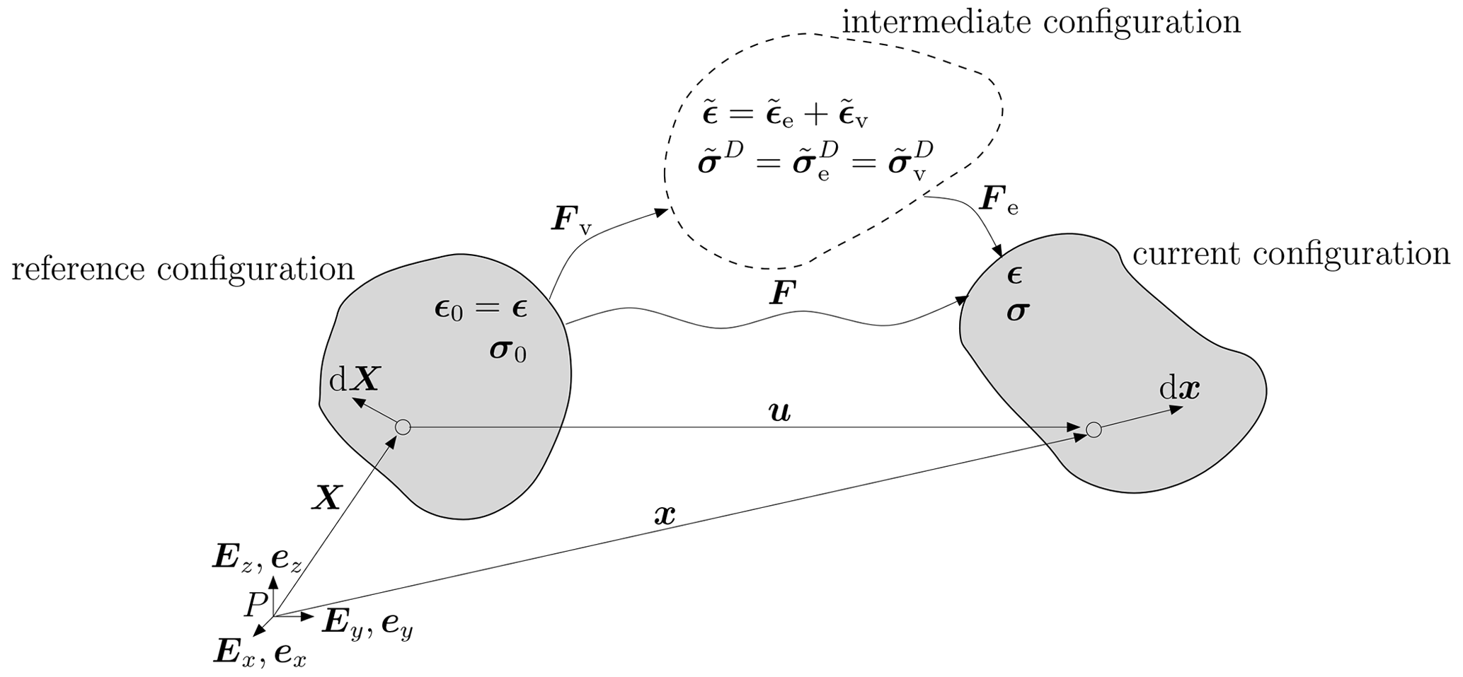
Figure B1Reference, current, and intermediate configurations and their corresponding strain and stress denotation for the finite viscoelastic Maxwell model. In the intermediate configuration (dashed line) the viscoelastic material equations are defined.
B2 Viscosity from inverse modeling
For estimating the viscosity distribution in the Filchner–Ronne Ice Shelf, we conduct a control-method inversion for the rheology parameter in the floating part using a non-Newtonian rheology with n=3. By this we mean that we invert for the ice-stiffness parameter B, more accurately for the vertically averaged rheology . We use the Ice-sheet and Sea-level System Model (Larour et al., 2012) applied to the Filchner–Ronne Ice Shelf using the Blatter–Pattyn higher-order approximation (Blatter, 1995; Pattyn, 2003). The calculation is done on an unstructured finite-element grid with a refined resolution of 2 km at the grounding line, in the shear margins as well as at other regions of faster ice flow. In the melt channel domain we further refine the resolution of the grid to 0.5 km.
To generate the geometry of the ice shelf the BedMachine Antarctica v2 data set is used (Morlighem et al., 2020; Morlighem, 2020). For the ice rigidity in the grounded region, as well as an initial guess of ice rigidity in the floating shelf, we assume the results of a long-term thermal spin-up also used in Eisen et al. (2020) based on the geothermal flux from Martos et al. (2017). We set Glen's flow-law exponent to n=3, and the viscosity η is described by the Cuffey temperate rheology law provided by ISSM. We constrain ice surface velocities to fit the MEaSUREs data set (Mouginot et al., 2019b, a).
Our optimization approach infers iteratively two parameters – the basal friction parameter k in the grounded area based on a linear sliding law and the ice vertically averaged rheology parameter in the floating area. For this purpose two cost functions are built. Each cost function consists of two data misfits evaluated at the surface S, linear and logarithmic, as well as a Tikhonov regularization term:
with vobs the observed surface velocity, v the modeled velocity, the respective control parameter for the inversion, and an added minimal velocity ξ to avoid singularities. The first term is most sensitive to velocity observations in fast-flowing areas, the second term is most sensitive to velocity observations in slow-floating areas and the third term Jreg(p) penalizes oscillations in the optimization parameter p. We performed an L-curve analysis to find suitable weights γ1, γ2 and γt for both cost functions. With this trade-off curve, we can make sure that we find a regularization term that fits the data well without overfitting noise. For the basal friction inversion, we found best weights γ1=1, and , while for the ice rigidity inversion the optimal weights were γ1=1, γ2=0.8 and .
We linearize and solve the optimization problem using the M1QN3 algorithm with an incomplete adjoint (Larour et al., 2012). The iterative optimization algorithm is considered to have converged if the adjoint gradient magnitude has dropped to a value less than times its initial value, if the normalized difference between successive solutions is less than , or if the maximum number of iterations (1000) is exceeded.
With the help of Glen's flow law the resulting rheology parameter from the inversion is used for calculating the effective viscosity:
where describes the effective strain rate. We show our best-fit results for ice viscosity in the region around the melt channel in Fig. B2. The range of the vertically averaged viscosity is between 5.0563×10¹³ and 2.6656×10¹⁵ Pa s.
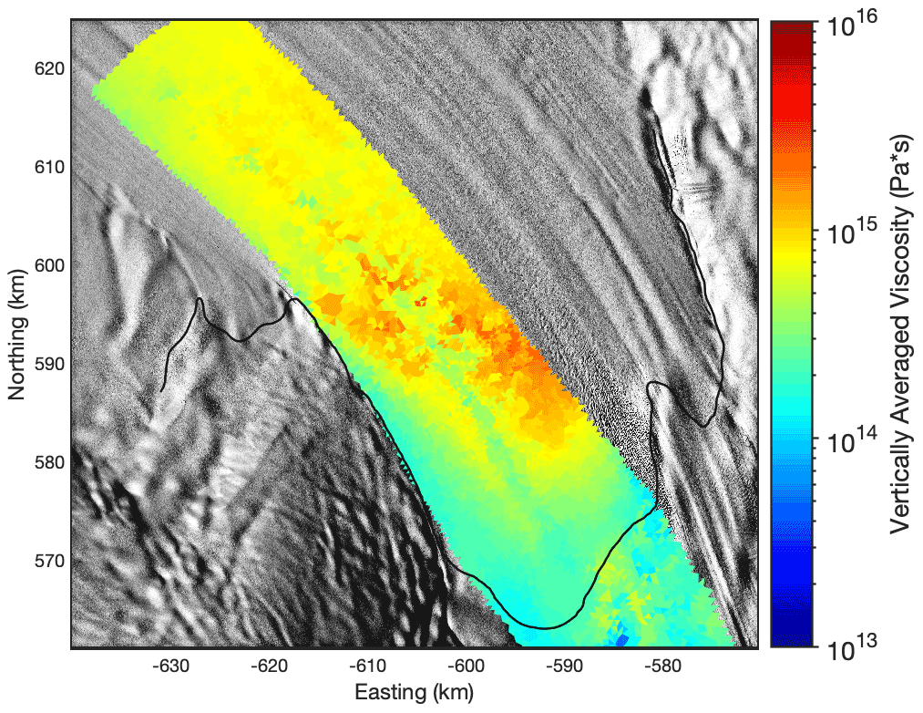
Figure B2Ice viscosity in the melt channel area obtained from inverse modeling. The map extent is the same as in Fig. 1. The background image is a hillshade of the Reference Elevation Model of Antarctica (Howat et al., 2018, 2019).
B3 Sensitivity of experiment 2 on viscosity
To capture the influence of the viscosity, different constant values (one smaller and one higher as in the second experiment) are investigated in a further experiment. The spin-up for each viscosity starts at years with a basal geometry that should fit the seismic IV profile at the end of the spin-up (t0). The melt rate is again assumed to be constant over the spin-up for all different viscosity values. We force the base with the synthetic melt rate (Fig. 3a), the same melt rate we already used in the second experiment. The initial base (at years) for the middle and high viscosity is nearly the same as 5×10¹⁵ Pa s is for ice a rather high value requiring cold ice (Fig. B8). For the smallest viscosity, a deeper channel at the beginning of the spin-up is needed.
B4 Elastic strain measure
For the concept of nonlinear strain, strain measures are defined and valid in particular configurations. However, the commonly used strain measures, like the Green–Lagrange strain in the reference configuration or the Euler–Almansi strain in the actual configuration, always have combined viscoelastic parts that cannot be split into viscous and elastic parts separately due to the multiplicative decomposition of the deformation gradient (Eq. B3). To quantify the elastic contribution of the melt channel evolution, we consider the Hencky strain, often called true strain, a logarithmic strain measure introduced in more detail by (Cuitino and Ortiz, 1992). Xiao (2005) and Neff et al. (2015) showed an extensive overview of the logarithmic strain properties and its applications. The advantage of the Hencky strain is an additive decomposition of the strain into an elastic and viscous part comparable to the procedure assuming a linearized strain for the linear strain theory. Furthermore, the Hencky strain is identical in the reference and current configuration.
The Hencky strain is defined by
We can compute the logarithm of the right Cauchy–Green tensor C by logarithmizing the eigenvalues derived by a spectral decomposition. For rigid body motions when C=I, the Hencky strain is zero. The eigenvalues of FTF for the Lagrangian perspective are the same as the eigenvalues of FFT in the Eulerian sense. Hence, the Hencky strain in the reference configuration is the same as in the current configuration, and, for simplicity, we call it strain ϵ here.
In the viscoelastic Maxwell model considering finite strains, we have a multiplicative decomposition of the deformation gradient F in an elastic and viscous part (Eq. B3), and it holds
with . Furthermore, we can split the deformation gradient in a rotation R and a stretching U (F=RU). The rotation has to be orthogonal; hence, we arbitrarily choose the viscous rotation as the identity tensor (Rv=I) and get
The stretching is symmetric , and we get based on the relation . In the end, we can split the strain additive into
and get the elastic strain
where Cv is the internal variable of the viscoelastic material model.
B5 Additional figures
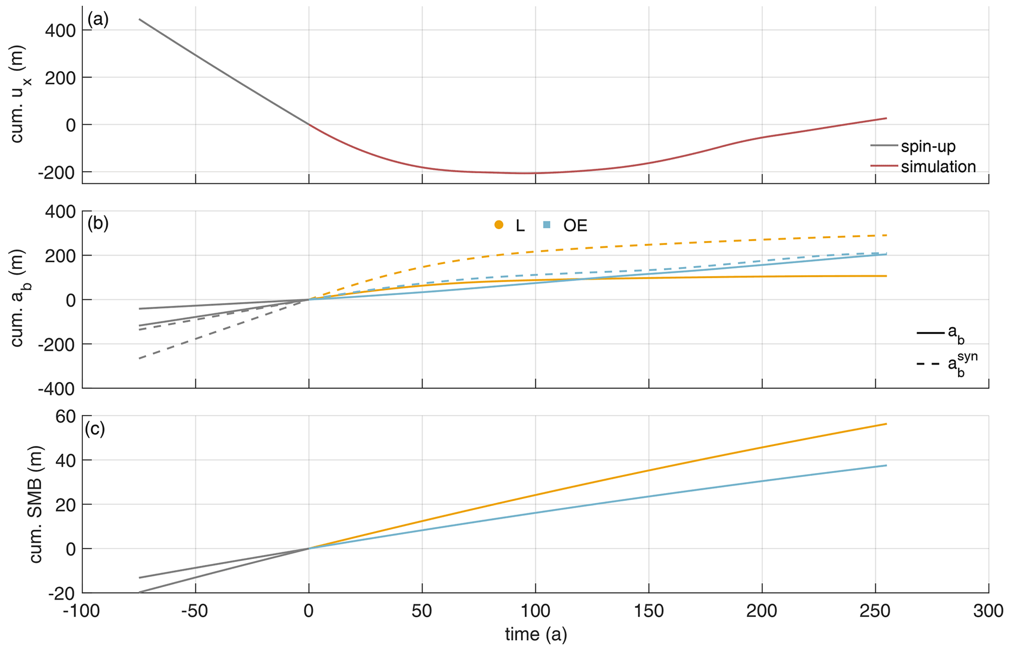
Figure B3Model input derived from pRES measurements and RACMO (van Wessem et al., 2014). (a) Cumulative horizontal displacement of the lateral boundaries calculated from pRES-derived vertical strain rates outside of the channel. (b) Cumulative basal melt rates above (yellow) and outside the channel (blue). Solid lines are derived from the pRES measurements, and dashed lines are synthetic melt rates that are necessary to reproduce the measured ice thickness distribution. (c) Cumulative surface mass balance (SMB) derived from multi-year mean RACMO2.3 data (van Wessem et al., 2014) for a density of 910 kg m−3 outside the channel (blue) and above the channel (yellow), 50 % larger. Gray lines represent values used in the spin-up and colored lines values used in the simulation of the evolution of the channel.
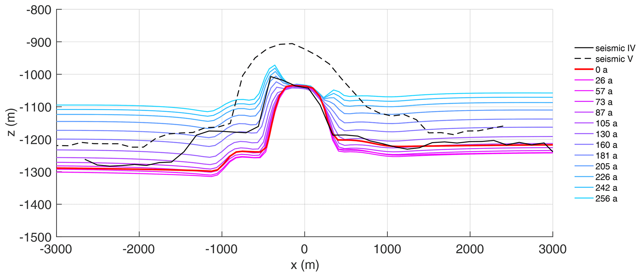
Figure B4Evolution of the base for the first experiment applying pRES-derived melt rates in the viscoelastic simulation. The black curve shows seismic profile IV (Hofstede et al., 2021b) and the red line the simulated base after the spin-up. For each position of pRES observations, the simulated base is shown using a color distribution ranging from red (furthest upstream) to blue (furthest downstream). The dashed black line is the base of seismic profile V (Hofstede et al., 2021b) near the pRES observation fitting to 130 years.
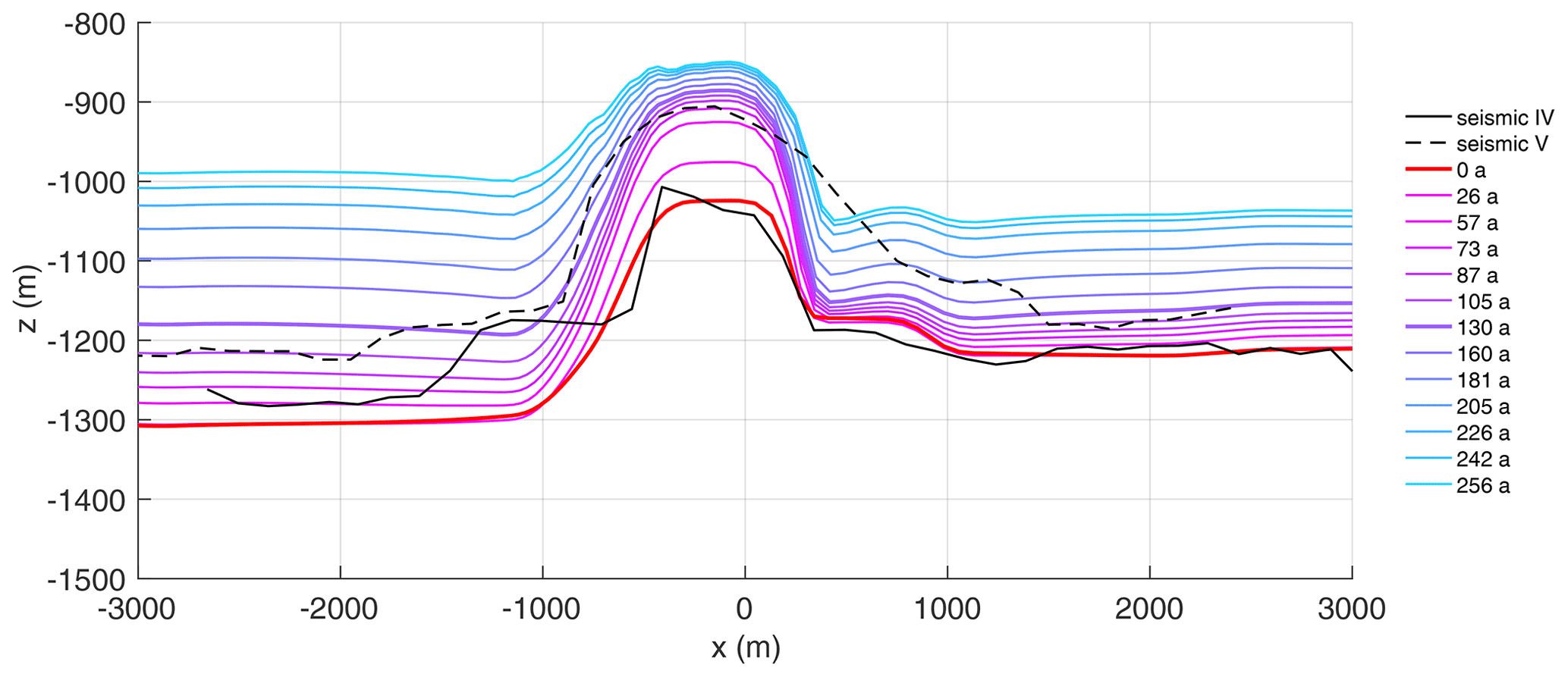
Figure B5Evolution of the base for the second experiment applying synthetic melt rates in the viscoelastic simulation. The black curve shows seismic profile IV (Hofstede et al., 2021b), and the red line is the simulated base after the spin-up. For each position of pRES observations, the simulated base is shown using a color distribution ranging from red (furthest upstream) to blue (furthest downstream). The dashed black line is the base of seismic profile V (Hofstede et al., 2021b) near the pRES observation fitting to 130 years. The opening of the basal channel cannot be rebuilt with the model as the melt rate inside the channel is only applied to constant channel width. The basal channel stays open during the simulation time of 256 years.
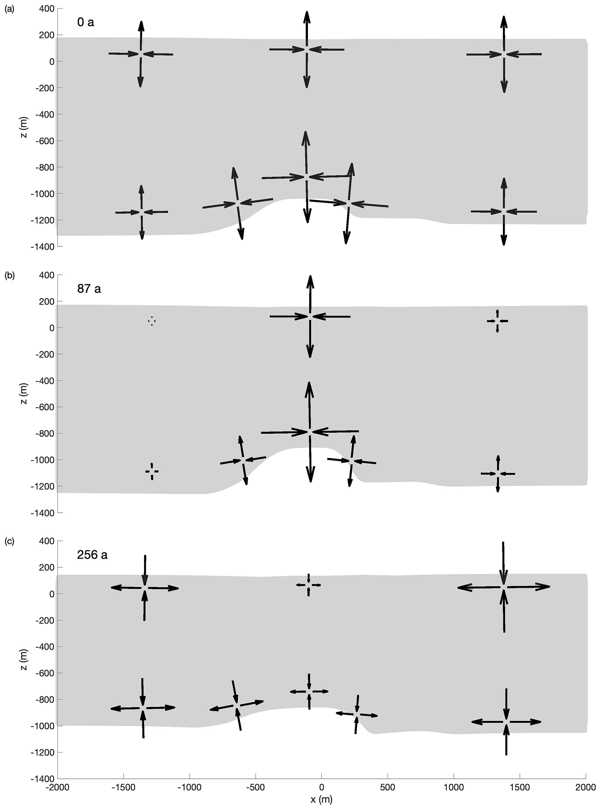
Figure B6Schematic arrows with their length according to the simulated principal strain magnitude and the pointing direction fitting to principal strain directions at specific points in the cross-section for three different points in time: (a) t=0 years (after the spin-up, maximum lateral compression), (b) t=87 years (small lateral displacement) and (c) t=256 years (end of the simulation).
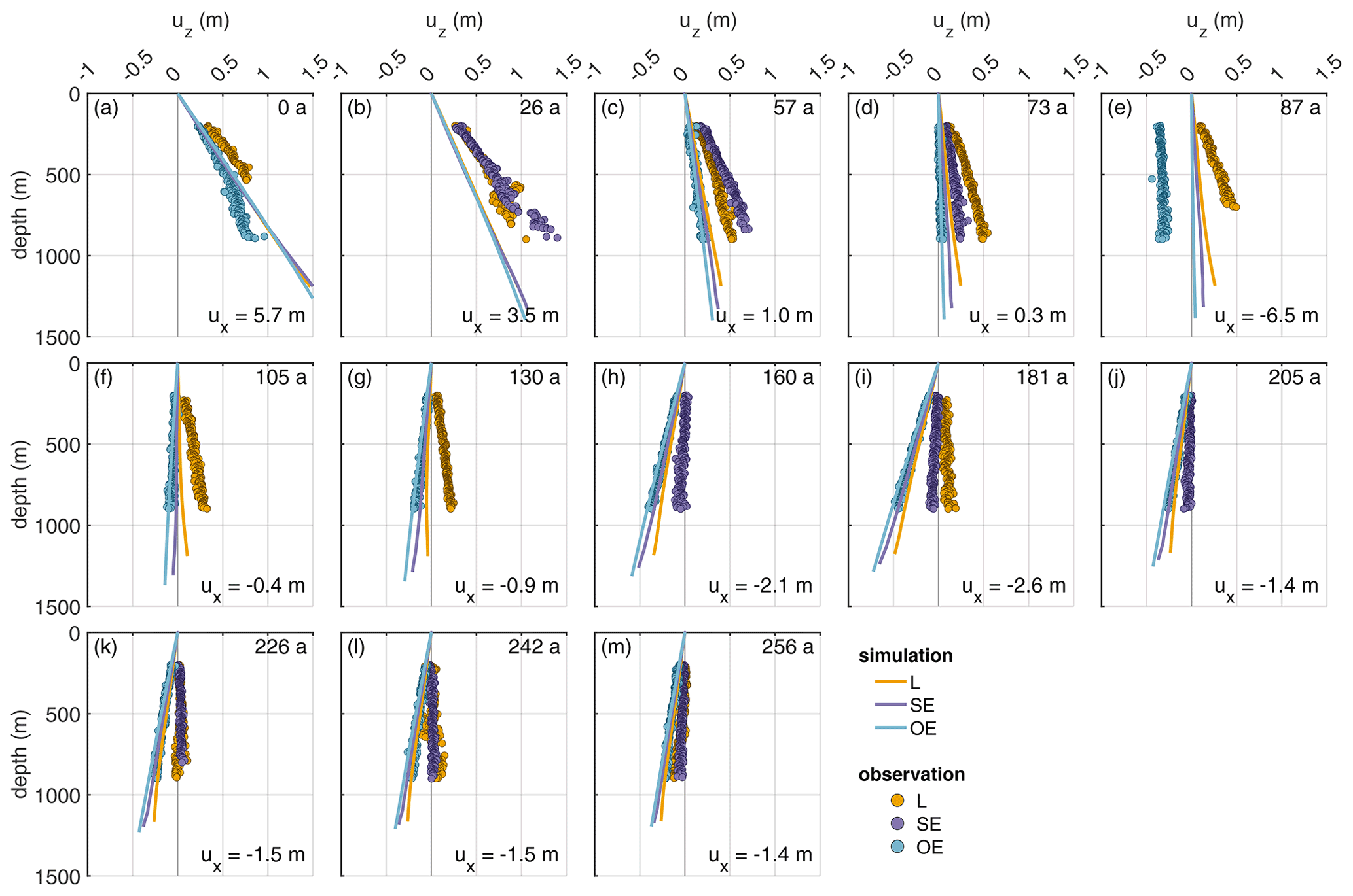
Figure B7First experiment: comparison of displacements (uz) derived from pRES measurements (dots) and from the simulations (lines). The different panels show the displacement for Δt=1 year allocated to the year of the model (number in upper right corner). The numbers in the lower right corners give horizontal displacement ux derived from εzz of the pRES measurements outside the channel (OE), with positive values representing compression and negative values extension.
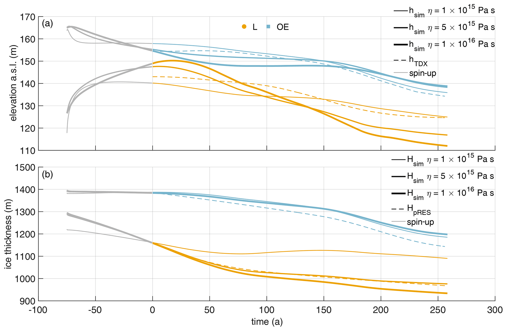
Figure B8(a) Surface elevation above the channel (yellow) and outside the channel (blue) derived from the simulation (solid lines) and from TanDEM-X DLR (2020) (dashed lines). (b) Ice thickness above the channel (yellow) and outside the channel (blue) derived from the simulation (solid lines) and from pRES measurements (dashed lines). The thickness of the solid lines represents the different viscosities: 1×10¹⁵ Pa s (thin line), 5×10¹⁵ Pa s (medium line, same value as in the second experiment) and 1×10¹⁶ Pa s (thick line). Gray lines represent values used in the spin-up and colored lines values used in the simulation of the evolution of the channel.
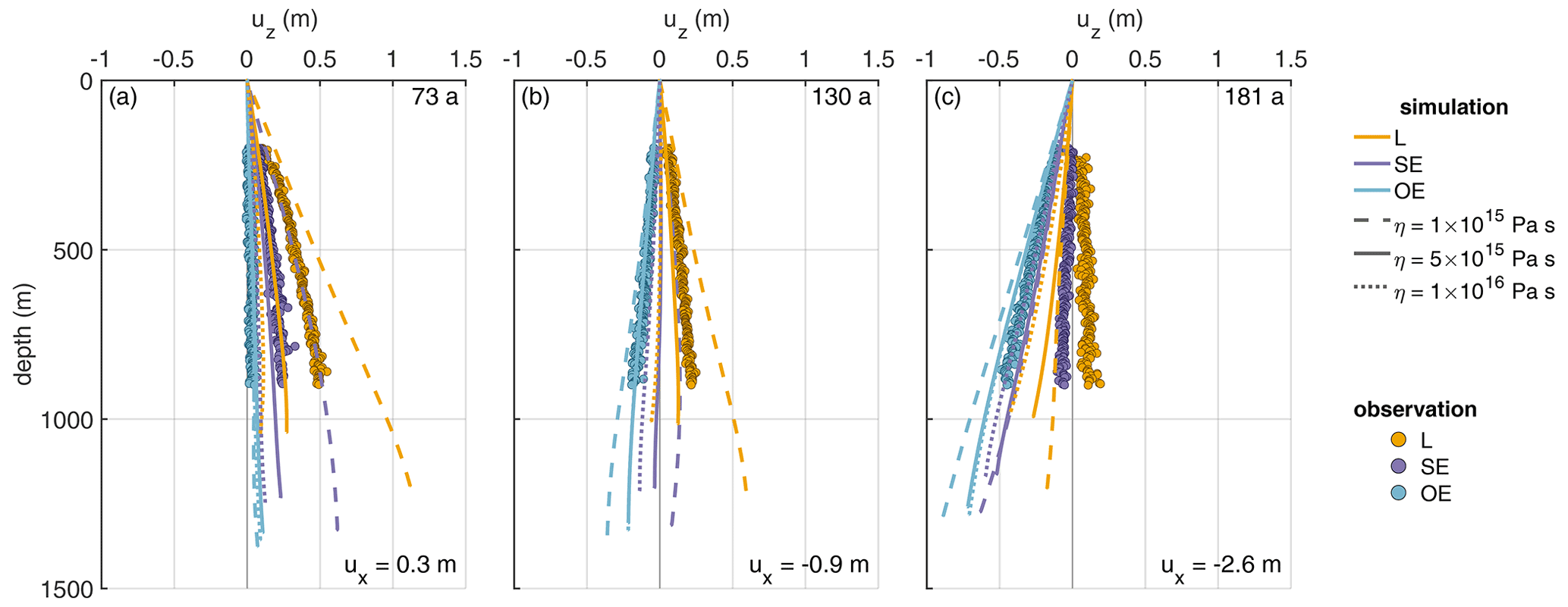
Figure B9Second experiment: comparison of displacements (uz) derived from observations (dots) and the simulations for different viscosities displayed by different line styles (lines). The different panels show the displacement for Δt=1 year allocated to the simulation time (upper right corner). The numbers in the lower right corners give horizontal displacement ux derived from εzz of the pRES measurements outside the channel (OE), with positive values representing compression and negative values extension.
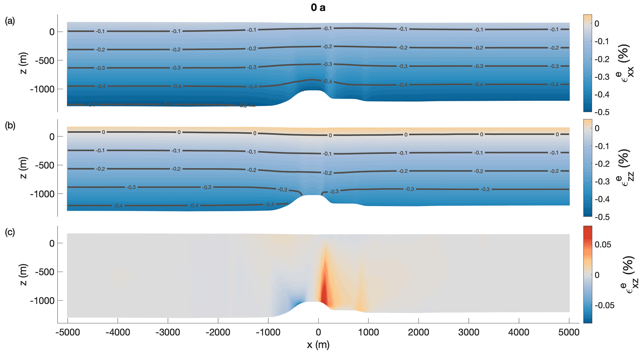
Figure B10The simulated elastic part of Hencky strain (a) in the across-flow direction and (b) in the vertical direction, and (c) the shear component for the second experiment using synthetic melt rates at t=0 year (after the spin-up, maximum lateral compression). The gray lines are contour lines of the elastic strain components. The normal components reach per mill values (the blueish colors denote compression), while the shear component is 1 order of magnitude smaller.
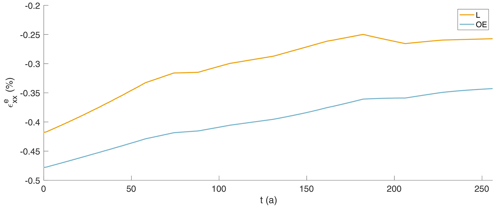
Figure B11The evolution of the simulated elastic part of Hencky strain at the ice base inside and outside the east of the channel in percent over the simulation time of 256 years. The initial elastic response of the grounded ice becoming afloat has vanished as the grounding line to far upstream. Avoiding model shocks with a spin-up of 75 years leads to a continuous Hencky strain at t=0 year.
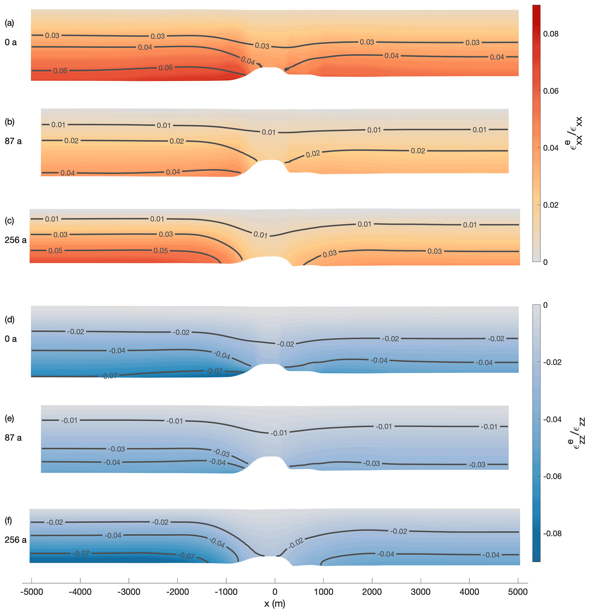
Figure B12Relative contribution of elastic to total strain of the second experiment using synthetic melt rates for the simulation. The upper three panels show the relative elastic strain in the across-flow direction for (a) t=0 year (after the spin-up, maximum lateral compression), (b) t=87 years (small lateral displacement) and (c) t=256 years (end of the simulation). The lower three panels show the relative elastic strain in the thickness direction for (d) t=0 year (after the spin-up, maximum lateral compression), (e) t=87 years (small lateral displacement) and (f) t=256 years (end of the simulation). The negative values denote that the elastic and viscous strains have different signs. The elastic and viscous Hencky strain sum up to the total strain.
The MPH file of the finite-element software COMSOL Multiphysics (version 5.6) of the viscoelastic finite strain simulation COMice-ve-fs used for this study is available via AWI's GitLab (https://gitlab.awi.de/jchristm/viscoelastic-finite-defos-meltchannel, last access: 5 October 2022, Christmann, 2022) or Zenodo (https://doi.org/10.5281/zenodo.7101449, Christmann et al., 2022).
Raw data and derived products of the single repeated pRES measurements (https://doi.org/10.1594/PANGAEA.941400, Zeising et al., 2022a), raw data of the ApRES time series (https://doi.org/10.1594/PANGAEA.932413, Zeising et al., 2021b), surface accumulation data at pRES locations (https://doi.org/10.1594/PANGAEA.940252, Zeising et al., 2021c) and processed GPS measurements (https://doi.org/10.1594/PANGAEA.932441, Zeising et al., 2021a) are published at the World Data Center PANGAEA. The seismic data (https://doi.org/10.1594/PANGAEA.932278) are available at the World Data Center PANGAEA (Hofstede et al., 2021b). The BedMachine Antarctica product can be accessed at https://doi.org/10.5067/E1QL9HFQ7A8M (Morlighem, 2020). The MEaSUREs velocity product can be accessed at https://doi.org/10.5067/PZ3NJ5RXRH10 (Mouginot et al., 2019a).
AH designed the study; conducted the field study together with DS; and wrote the manuscript together with OZ, JC, KWN, VH and LSH. OZ processed the pRES/ApRES data and analyzed the melt rates together with AH. JC performed the viscoelastic simulations together with TS and with contributions from OZ and AH. JC, AH and OZ analyzed the results together with RM. VH and OZ processed the GPS data. LSH and MW performed the inverse modeling. CH performed the seismic measurements and supported the discussions. NN calculated the TDX DEM. KWN supported the field study and contributed to melt rate analysis and its discussion together with HFJC. All authors helped to improve writing.
The contact author has declared that none of the authors has any competing interests.
Publisher's note: Copernicus Publications remains neutral with regard to jurisdictional claims in published maps and institutional affiliations.
This work was funded by the AWI strategy fund project FISP. We acknowledge the support of BAS for the field campaign, in particular the support of the Graham Niven and Bradley Morell, who have been field assistants in the two expeditions. Lea-Sophie Höyns is funded through the Helmholtz School for Marine Data Science (MarDATA) (grant no. HIDSS-0005). Support for this work came from the UK Natural Environment Research Council large grant “Ice shelves in a warming world: Filchner Ice Shelf system” (NE/L013770/1).
This research has been supported by the Alfred Wegener Institute Helmholtz Centre for Polar and Marine Research (Strategy Fund FISP), the Helmholtz-Gemeinschaft (grant no. HIDSS-0005), and the Natural Environment Research Council British Antarctic Survey (grant no. NE/L013770/1).
The article processing charges for this open-access publication were covered by the Alfred Wegener Institute, Helmholtz Centre for Polar and Marine Research (AWI).
This paper was edited by Elisa Mantelli and reviewed by two anonymous referees.
Alley, K. E., Scambos, T. A., Alley, R. B., and Holschuh, N.: Troughs developed in ice-stream shear margins precondition ice shelves for ocean-driven breakup, Science Advances, 5, eaax2215, https://doi.org/10.1126/sciadv.aax2215, 2019. a
Bassis, J. and Ma, Y.: Evolution of basal crevasses links ice shelf stability to ocean forcing, Earth Planetary Sc. Lett., 409, 203–211, https://doi.org/10.1016/j.epsl.2014.11.003, 2015. a
Blatter, H.: Velocity and stress fields in grounded glaciers: a simple algorithm for including deviatoric stress gradients, J. Glaciol., 41, 333–344, https://doi.org/10.3189/S002214300001621X, 1995. a, b
Brennan, P. V., Lok, L. B., Nicholls, K., and Corr, H.: Phase-sensitive FMCW radar system for high-precision Antarctic ice shelf profile monitoring, IET Radar Sonar Nav., 8, 776–786, https://doi.org/10.1049/iet-rsn.2013.0053, 2014. a, b
Christmann, J.: Viscoelastic Finite Strain Meltchannel, AWI GitLab [code], https://gitlab.awi.de/jchristm/viscoelastic-finite-defos-meltchannel, last access: 5 October 2022. a
Christmann, J., Plate, C., Müller, R., and Humbert, A.: Viscous and viscoelastic stress states at the calving front of Antarctic ice shelves, Ann. Glaciol., 57, 10–18, https://doi.org/10.1017/aog.2016.18, 2016. a
Christmann, J., Müller, R., and Humbert, A.: On nonlinear strain theory for a viscoelastic material model and its implications for calving of ice shelves, J. Glaciol., 65, 212–224, https://doi.org/10.1017/jog.2018.107, 2019. a, b, c, d
Christmann, J., Helm, V., Khan, S. A., Kleiner, T., Müller, R., Morlighem, M., Neckel, N., Rückamp, M., Steinhage, D., Zeising, O., and Humbert, A.: Elastic deformation plays a non-negligible role in Greenland's outlet glacier flow, Communications Earth & Environment, 2, 232, https://doi.org/10.1038/s43247-021-00296-3, 2021. a, b
Christmann, J., Humbert, A., Schultz, T., and Müller, R.: COMice-ve-fs as used in Humbert et al., The Cyrosphere, Version 1, Zenodo [code], https://doi.org/10.5281/zenodo.7101449, 2022. a
Corr, H. F., Jenkins, A., Nicholls, K. W., and Doake, C.: Precise measurement of changes in ice-shelf thickness by phase-sensitive radar to determine basal melt rates, Geophys. Res. Lett., 29, 73-1–73-4, https://doi.org/10.1029/2001GL014618, 2002. a
Cuitino, A. and Ortiz, M.: Computational modelling of single crystals, Model. Simul. Mater. Sc., 1, 225–263, https://doi.org/10.1088/0965-0393/1/3/001, 1992. a
Dinniman, M. S., Asay-Davis, X. S., Galton-Fenzi, B. K., Holland, P. R., Jenkins, A., and Timmermann, R.: Modeling Ice Shelf/Ocean Interaction in Antarctica: A Review, Oceanography, 29, 144–153, https://doi.org/10.5670/oceanog.2016.106, 2016. a
DLR (German Aerospace Center): TanDEM-X - PolarDEM - Antarctica, 90m, DLR [data set], https://doi.org/10.15489/9jhr18jepi65, 2020. a, b
Dow, C. F., Lee, W. S., Greenbaum, J. S., Greene, C. A., Blankenship, D. D., Poinar, K., Forrest, A. L., Young, D. A., and Zappa, C. J.: Basal channels drive active surface hydrology and transverse ice shelf fracture, Science Advances, 4, eaao7212, https://doi.org/10.1126/sciadv.aao7212, 2018. a, b, c
Drews, R.: Evolution of ice-shelf channels in Antarctic ice shelves, The Cryosphere, 9, 1169–1181, https://doi.org/10.5194/tc-9-1169-2015, 2015. a
Drews, R., Pattyn, F., Hewitt, I. J., Ng, F. S. L., Berger, S., Matsuoka, K., Helm, V., Bergeot, N., Favier, L., and Neckel, N.: Actively evolving subglacial conduits and eskers initiate ice shelf channels at an Antarctic grounding line, Nat. Commun., 8, 15228, https://doi.org/10.1038/ncomms15228, 2017. a
Dutrieux, P., Stewart, C., Jenkins, A., Nicholls, K. W., Corr, H. F., Rignot, E., and Steffen, K.: Basal terraces on melting ice shelves, Geophys. Res. Lett., 41, 5506–5513, https://doi.org/10.1002/2014GL060618, 2014. a, b
Eisen, O., Winter, A., Steinhage, D., Kleiner, T., and Humbert, A.: Basal roughness of the East Antarctic Ice Sheet in relation to flow speed and basal thermal state, Ann. Glaciol., 61, 162–175, https://doi.org/10.1017/aog.2020.47, 2020. a, b
Foerste, C., Bruinsma, S., Abrykosov, O., Lemoine, J.-M., Marty, J. C., Flechtner, F., Balmino, G., Barthelmes, F., and Biancale, R.: EIGEN-6C4 The latest combined global gravity field model including GOCE data up to degree and order 2190 of GFZ Potsdam and GRGS Toulouse, GFZ Data Services [data set], https://doi.org/10.5880/icgem.2015.1, 2014. a
Fujita, S., Matsuoka, T., Ishida, T., Matsuoka, K., and Mae, S.: A summary of the complex dielectric permittivity of ice in the megahertz range and its applications for radar sounding of polar ice sheets, in: Physics of ice core records, Hokkaido University Press, 185–212, http://hdl.handle.net/2115/32469 (last access: 29 September 2022), 2000. a
Galton-Fenzi, B. K., Hunter, J. R., Coleman, R., Marsland, S. J., and Warner, R. C.: Modeling the basal melting and marine ice accretion of the Amery Ice Shelf, J. Geophys. Res.-Oceans, 117, C09031, https://doi.org/10.1029/2012JC008214, 2012. a
Gladish, C. V., Holland, D. M., Holland, P. R., and Price, S. F.: Ice-shelf basal channels in a coupled ice/ocean model, J. Glaciol., 58, 1227–1244, https://doi.org/10.3189/2012JoG12J003, 2012. a
Gudmundsson, G. H.: Ice-stream response to ocean tides and the form of the basal sliding law, The Cryosphere, 5, 259–270, https://doi.org/10.5194/tc-5-259-2011, 2011. a
Gwyther, D. E., Kusahara, K., Asay-Davis, X. S., Dinniman, M. S., and Galton-Fenzi, B. K.: Vertical processes and resolution impact ice shelf basal melting: A multi-model study, Ocean Model., 147, 101569, https://doi.org/10.1016/j.ocemod.2020.101569, 2020. a
Haupt, P.: Continuum Mechanics and Theory of Materials, Springer, Berlin, https://doi.org/10.1007/978-3-662-04775-0, 2000. a, b, c
Helm, V., Humbert, A., and Miller, H.: Elevation and elevation change of Greenland and Antarctica derived from CryoSat-2, The Cryosphere, 8, 1539–1559, https://doi.org/10.5194/tc-8-1539-2014, 2014. a
Herron, M. M. and Langway, C. C.: Firn densification: an empirical model, J. Glaciol., 25, 373–385, https://doi.org/10.3189/S0022143000015239, 1980. a, b
Hofstede, C., Beyer, S., Corr, H., Eisen, O., Hattermann, T., Helm, V., Neckel, N., Smith, E. C., Steinhage, D., Zeising, O., and Humbert, A.: Evidence for a grounding line fan at the onset of a basal channel under the ice shelf of Support Force Glacier, Antarctica, revealed by reflection seismics, The Cryosphere, 15, 1517–1535, https://doi.org/10.5194/tc-15-1517-2021, 2021a. a, b, c, d, e, f, g
Hofstede, C., Beyer, S., Corr, H. F. J., Eisen, O., Hattermann, T., Helm, V., Neckel, N., Smith, E. C., Steinhage, D., Zeising, O., and Humbert, A.: Seismic reflection data of a basal channel and ocean cavity at the ice shelf-grounding line area of Support Force Glacier, Filchner Ice Shelf, Antarctica, PANGAEA [data set],https://doi.org/10.1594/PANGAEA.932278, 2021b. a, b, c, d, e, f, g
Holland, D. M. and Jenkins, A.: Modeling Thermodynamic Ice–Ocean Interactions at the Base of an Ice Shelf, J. Phys. Oceanogr., 29, 1787–1800, https://doi.org/10.1175/1520-0485(1999)029<1787:MTIOIA>2.0.CO;2, 1999. a
Holland, P. R. and Kwok, R.: Wind-driven trends in Antarctic sea-ice drift, Nat. Geosci., 5, 872–875, https://doi.org/10.1038/ngeo1627, 2012. a
Howat, I., Morin, P., Porter, C., and Noh, M.-J.: The Reference Elevation Model of Antarctica, Version V1, Harvard Dataverse [data set], https://doi.org/10.7910/DVN/SAIK8B, 2018. a, b
Howat, I. M., Porter, C., Smith, B. E., Noh, M.-J., and Morin, P.: The Reference Elevation Model of Antarctica, The Cryosphere, 13, 665–674, https://doi.org/10.5194/tc-13-665-2019, 2019. a, b
Humbert, A., Steinhage, D., Helm, V., Hoerz, S., Berendt, J., Leipprand, E., Christmann, J., Plate, C., and Müller, R.: On the link between surface and basal structures of the Jelbart Ice Shelf, Antarctica, J. Glaciol., 61, 975–986, https://doi.org/10.3189/2015JoG15J023, 2015. a, b
Humbert, A., Steinhage, D., Helm, V., Beyer, S., and Kleiner, T.: Missing evidence of widespread subglacial lakes at Recovery Glacier, Antarctica, J. Geophys. Res.-Earth, 123, 2802–2826, https://doi.org/10.1029/2017JF004591, 2018. a, b
Jenkins, A. and Doake, C.: Ice-ocean interaction on Ronne Ice Shelf, Antarctica, J. Geophys. Res.-Oceans, 96, 791–813, https://doi.org/10.1029/90JC01952, 1991. a
Jenkins, A., Corr, H. F., Nicholls, K. W., Stewart, C. L., and Doake, C. S.: Interactions between ice and ocean observed with phase-sensitive radar near an Antarctic ice-shelf grounding line, J. Glaciol., 52, 325–346, https://doi.org/10.3189/172756506781828502, 2006. a, b, c, d
Jeofry, H., Ross, N., Le Brocq, A., Graham, A. G. C., Li, J., Gogineni, P., Morlighem, M., Jordan, T., and Siegert, M. J.: Hard rock landforms generate 130 km ice shelf channels through water focusing in basal corrugations, Nat. Commun., 8, 4576, https://doi.org/10.1038/s41467-018-06679-z, 2018. a
Jourdain, N. C., Mathiot, P., Merino, N., Durand, G., Le Sommer, J., Spence, P., Dutrieux, P., and Madec, G.: Ocean circulation and sea-ice thinning induced by melting ice shelves in the Amundsen Sea, J. Geophys. Res.-Oceans, 122, 2550–2573, https://doi.org/10.1002/2016JC012509, 2017. a
Kovacs, A., Gow, A. J., and Morey, R. M.: The in-situ dielectric constant of polar firn revisited, Cold Reg. Sci. Technol., 23, 245–256, https://doi.org/10.1016/0165-232X(94)00016-Q, 1995. a
Langley, K., von Deschwanden, A., Kohler, J., Sinisalo, A., Matsuoka, K., Hattermann, T., Humbert, A., Nøst, O., and Isaksson, E.: Complex network of channels beneath an Antarctic ice shelf, Geophys. Res. Lett., 41, 1209–1215, https://doi.org/10.1002/2013GL058947, 2014. a, b, c, d
Larour, E., Seroussi, H., Morlighem, M., and Rignot, E.: Continental scale, high order, high spatial resolution, ice sheet modeling using the Ice Sheet System Model (ISSM), J. Geophys. Res.-Earth, 117, F01022, https://doi.org/10.1029/2011JF002140, 2012. a, b, c
Le Brocq, A. M., Ross, N., Griggs, J. A., Bingham, R. G., Corr, H. F., Ferraccioli, F., Jenkins, A., Jordan, T. A., Payne, A. J., Rippin, D. M., and Siegert, M. J.: Evidence from ice shelves for channelized meltwater flow beneath the Antarctic Ice Sheet, Nat. Geosci., 6, 945–948, https://doi.org/10.1038/ngeo1977, 2013. a, b, c, d, e, f
Lee, E. H.: Elastic-plastic deformation at finite strains, J. Appl. Mech., 36, 1–6, https://doi.org/10.1115/1.3564580, 1969. a
Lindbäck, K., Moholdt, G., Nicholls, K. W., Hattermann, T., Pratap, B., Thamban, M., and Matsuoka, K.: Spatial and temporal variations in basal melting at Nivlisen ice shelf, East Antarctica, derived from phase-sensitive radars, The Cryosphere, 13, 2579–2595, https://doi.org/10.5194/tc-13-2579-2019, 2019. a
MacAyeal, D. R.: Thermohaline circulation below the Ross Ice Shelf: A consequence of tidally induced vertical mixing and basal melting, J. Geophys. Res.-Oceans, 89, 597–606, https://doi.org/10.1029/JC089iC01p00597, 1984. a
Marsh, O. J., Fricker, H. A., Siegfried, M. R., Christianson, K., Nicholls, K. W., Corr, H. F., and Catania, G.: High basal melting forming a channel at the grounding line of Ross Ice Shelf, Antarctica, Geophys. Res. Lett., 43, 250–255, https://doi.org/10.1002/2015GL066612, 2016. a, b, c, d
Martos, Y. M., Catalán, M., Jordan, T. A., Golynsky, A., Golynsky, D., Eagles, G., and Vaughan, D. G.: Heat Flux Distribution of Antarctica Unveiled, Geophys. Res. Lett., 44, 11417–11426, https://doi.org/10.1002/2017GL075609, 2017. a, b
Millgate, T., Holland, P. R., Jenkins, A., and Johnson, H. L.: The effect of basal channels on oceanic ice-shelf melting, J. Geophys. Res.-Oceans, 118, 6951–6964, https://doi.org/10.1002/2013JC009402, 2013. a
Morlighem, M.: MEaSUREs BedMachine Antarctica, Version 2, NASA National Snow and Ice Data Center Distributed Active Archive Center [data set], Boulder, Colorado, USA, https://doi.org/10.5067/E1QL9HFQ7A8M, 2020. a, b, c
Morlighem, M., Rignot, E., Binder, T., Blankenship, D., Drews, R., Eagles, G., Eisen, O., Ferraccioli, F., Forsberg, R., Fretwell, P., Goel, V., Greenbaum, J. S., Gudmundsson, H., Guo, J., Helm, V., Hofstede, C., Howat, I., Humbert, A., Jokat, W., Karlsson, N. B., Lee, W. S., Matsuoka, K., Millan, R., Mouginot, J., Paden, J., Pattyn, F., Roberts, J., Rosier, S., Ruppel, A., Seroussi, H., Smith, E. C., Steinhage, D., Sun, B., van den Broeke, M. R., van Ommen, T. D., van Wessem, M., and Young, D. A.: Deep glacial troughs and stabilizing ridges unveiled beneath the margins of the Antarctic ice sheet, Nat. Geosci., 13, 132–137, https://doi.org/10.1038/s41561-019-0510-8, 2020. a, b
Mouginot, J., Rignot, E., and Scheuchl, B.: MEaSUREs Phase-Based Antarctica Ice Velocity Map, Version 1, NASA National Snow and Ice Data Center Distributed Active Archive Center [data set], Boulder, Colorado, USA, https://doi.org/10.5067/PZ3NJ5RXRH10, 2019a. a, b, c
Mouginot, J., Rignot, E., and Scheuchl, B.: Continent-Wide, Interferometric SAR Phase, Mapping of Antarctic Ice Velocity, Geophys. Res. Lett., 46, 9710–9718, https://doi.org/10.1029/2019GL083826, 2019b. a, b
Naughten, K. A., De Rydt, J., Rosier, S. H. R., Jenkins, A., Holland, P. R., and Ridley, J. K.: Two-timescale response of a large Antarctic ice shelf to climate change, Nat. Commun., 12, 1991, https://doi.org/10.1038/s41467-021-22259-0, 2021. a
Neff, P., Ghiba, I.-D., and Lankeit, J.: The exponentiated Hencky-logarithmic strain energy. Part I: constitutive issues and rank-one convexity, J. Elasticity, 121, 143–234, https://doi.org/10.1007/s10659-015-9524-7, 2015. a
Nicholls, K. W.: Predicted reduction in basal melt rates of an Antarctic ice shelf in a warmer climate, Nature, 388, 460–462, https://doi.org/10.1038/41302, 1997. a, b
Nicholls, K. W.: The study of ice shelf-ocean interaction—techniques and recent results, Advances in Polar Science, 3, 222–230, https://doi.org/10.13679/j.advps.2018.3.00222, 2018. a
Nicholls, K. W., Corr, H. F., Stewart, C. L., Lok, L. B., Brennan, P. V., and Vaughan, D. G.: A ground-based radar for measuring vertical strain rates and time-varying basal melt rates in ice sheets and shelves, J. Glaciol., 61, 1079–1087, https://doi.org/10.3189/2015JoG15J073, 2015. a, b
Pattyn, F.: A new three-dimensional higher-order thermomechanical ice sheet model: Basic sensitivity, ice stream development, and ice flow across subglacial lakes, J. Geophys. Res.-Sol. Ea., 108, 2382, https://doi.org/10.1029/2002JB002329, 2003. a, b
Reeh, N., Mayer, C., Olesen, O. B., Christensen, E. L., and Thomsen, H. H.: Tidal movement of Nioghalvfjerdsfjorden glacier, northeast Greenland: observations and modelling, Ann. Glaciol., 31, 111–117, https://doi.org/10.3189/172756400781820408, 2000. a
Rignot, E. and Steffen, K.: Channelized bottom melting and stability of floating ice shelves, Geophys. Res. Lett., 35, L02503, https://doi.org/10.1029/2007GL031765, 2008. a, b
Rizzoli, P., Martone, M., Gonzalez, C., Wecklich, C., Borla Tridon, D., Bräutigam, B., Bachmann, M., Schulze, D., Fritz, T., Huber, M., Wessel, B., Krieger, G., Zink, M., and Moreira, A.: Generation and performance assessment of the global TanDEM-X digital elevation model, ISPRS J. Photogramm., 132, 119–139, https://doi.org/10.1016/j.isprsjprs.2017.08.008, 2017. a, b
Schultz, T.: Viskoelastische Modellierung der Dynamik eines Gletschers als Antwort auf basales Schmelzen und die Oberflächenmassenbilanz, Master thesis, https://doi.org/10.26092/elib/1777, 2017. a
Sergienko, O.: Basal channels on ice shelves, J. Geophys. Res.-Earth, 118, 1342–1355, https://doi.org/10.1002/jgrf.20105, 2013. a
Seroussi, H., Nakayama, Y., Larour, E., Menemenlis, D., Morlighem, M., Rignot, E., and Khazendar, A.: Continued retreat of Thwaites Glacier, West Antarctica, controlled by bed topography and ocean circulation, Geophys. Res. Lett., 44, 6191–6199, https://doi.org/10.1002/2017GL072910, 2017. a
Smith, B. E., Fricker, H. A., Joughin, I. R., and Tulaczyk, S.: An inventory of active subglacial lakes in Antarctica detected by ICESat (2003–2008), J. Glaciol., 55, 573–595, https://doi.org/10.3189/002214309789470879, 2009. a
Stanton, T., Shaw, W., Truffer, M., Corr, H., Peters, L., Riverman, K., Bindschadler, R., Holland, D., and Anandakrishnan, S.: Channelized ice melting in the ocean boundary layer beneath Pine Island Glacier, Antarctica, Science, 341, 1236–1239, https://doi.org/10.1126/science.1239373, 2013. a
Stewart, C. L., Christoffersen, P., Nicholls, K. W., Williams, M. J., and Dowdeswell, J. A.: Basal melting of Ross Ice Shelf from solar heat absorption in an ice-front polynya, Nat. Geosci., 12, 435, https://doi.org/10.1038/s41561-019-0356-0, 2019. a, b, c
Sun, S., Hattermann, T., Pattyn, F., Nicholls, K. W., Drews, R., and Berger, S.: Topographic shelf waves control seasonal melting near Antarctic ice shelf grounding lines, Geophys. Res. Lett., 46, 9824–9832, 2019. a
Timmermann, R. and Hellmer, H.: Southern Ocean warming and increased ice shelf basal melting in the twenty-first and twenty-second centuries based on coupled ice-ocean finite-element modelling, Ocean Dynam., 63, 1011–1026, https://doi.org/10.1007/s10236-013-0642-0, 2013. a
Vaňková, I., Nicholls, K. W., Corr, H. F., Makinson, K., and Brennan, P. V.: Observations of tidal melt and vertical strain at the Filchner-Ronne Ice Shelf, Antarctica, J. Geophys. Res.-Earth, 125, e2019JF005280, https://doi.org/10.1029/2019JF005280, 2020. a, b, c, d, e, f, g, h
Vaňková, I., Nicholls, K. W., and Corr, H. F. J.: The Nature of Ice Intermittently Accreted at the Base of Ronne Ice Shelf, Antarctica, Assessed Using Phase-Sensitive Radar, J. Geophys. Res.-Oceans, 126, e2021JC017290, https://doi.org/10.1029/2021JC017290, 2021. a
van Wessem, J., Reijmer, C., Morlighem, M., Mouginot, J., Rignot, E., Medley, B., Joughin, I., Wouters, B., Depoorter, M., Bamber, J., Lenaerts, J. T. M., Van De Berg, W. J., Van Den Broeke, M. R., and Van Meijgaard, E.: Improved representation of East Antarctic surface mass balance in a regional atmospheric climate model, J. Glaciol., 60, 761–770, https://doi.org/10.3189/2014JoG14J051, 2014. a, b, c, d, e
Vaughan, D. G., Corr, H. F., Bindschadler, R. A., Dutrieux, P., Gudmundsson, G. H., Jenkins, A., Newman, T., Vornberger, P., and Wingham, D. J.: Subglacial melt channels and fracture in the floating part of Pine Island Glacier, Antarctica, J. Geophys. Res.-Earth, 117, F03012, https://doi.org/10.1029/2012JF002360, 2012. a
Washam, P., Nicholls, K. W., Münchow, A., and Padman, L.: Summer surface melt thins Petermann Gletscher Ice Shelf by enhancing channelized basal melt, J. Glaciol., 65, 662–674, https://doi.org/10.1017/jog.2019.43, 2019. a
Wearing, M. G., Stevens, L. A., Dutrieux, P., and Kingslake, J.: Ice-Shelf Basal Melt Channels Stabilized by Secondary Flow, Geophys. Res. Lett., 48, e2021GL094872, https://doi.org/10.1029/2021GL094872, 2021. a, b
Xiao, H.: Hencky strain and Hencky model: extending history and ongoing tradition, Multidiscipline Modeling in Materials and Structures, 1, 1–52, https://doi.org/10.1163/1573611054455148, 2005. a
Zeising, O. and Humbert, A.: Indication of high basal melting at the EastGRIP drill site on the Northeast Greenland Ice Stream, The Cryosphere, 15, 3119–3128, https://doi.org/10.5194/tc-15-3119-2021, 2021. a, b, c
Zeising, O., Helm, V., Steinhage, D., and Humbert, A.: GNSS measurements at a basal melt channel of the southern Filchner Ice Shelf, Antarctica, PANGAEA [data set], https://doi.org/10.1594/PANGAEA.932441, 2021a. a
Zeising, O., Steinhage, D., and Humbert, A.: Autonomous phase-sensitive radar (ApRES) measurements at a basal melt channel of the southern Filchner Ice Shelf, Antarctica between 2016/17 and 2017/18, PANGAEA [data set], https://doi.org/10.1594/PANGAEA.932413, 2021b. a
Zeising, O., Steinhage, D., and Humbert, A.: Stake surface accumulation measurements at Filchnner Ice Shelf between December 2015/January 2016 and December 2016, PANGAEA [data set], https://doi.org/10.1594/PANGAEA.940252, 2021c. a
Zeising, O., Steinhage, D., and Humbert, A.: Melt rates of 44 repeated phase-sensitive radar point measurements between December 2015/January 2016 and December 2016 at the Filchner Ice Shelf, Antarctica, PANGAEA [data set], https://doi.org/10.1594/PANGAEA.941400, 2022a. a
Zeising, O., Steinhage, D., Nicholls, K. W., Corr, H. F. J., Stewart, C. L., and Humbert, A.: Basal melt of the southern Filchner Ice Shelf, Antarctica, The Cryosphere, 16, 1469–1482, https://doi.org/10.5194/tc-16-1469-2022, 2022b. a, b