Topology and spatial-pressure-distribution reconstruction of an englacial channel

Information about glacier hydrology is important for understanding glacier and ice sheet dynamics. However, our knowledge about water pathways and pressure remains limited, as in situ observations are sparse and methods for direct area-wide observations are limited due to the extreme and hard-to-access nature of the environment. In this paper, we present a method that allows for in situ data collection in englacial channels using sensing drifters. Furthermore, we demonstrate a model that takes the collected data and reconstructs the planar subsurface water flow paths providing spatial reference to the continuous water pressure measurements. We showcase this method by reconstructing the 2D topology and the water pressure distribution of a free-flowing englacial channel in Austre Brøggerbreen (Svalbard). The approach uses inertial measurements from submersible sensing drifters and reconstructs the water flow path between given start and end coordinates. Validation of the method was done on a separate supraglacial channel, showing an average error of 3.9 m and the total channel length error of 29 m (6.5 %). At the englacial channel, the average error is 12.1 m; the length error is 107 m (11.6 %); and the water pressure standard deviation is 3.4 hPa (0.3 %). Our method allows for mapping of subsurface water flow paths and spatially referencing the pressure distribution within. Further, our method would be extendable to the reconstruction of other, previously underexplored subsurface fluid flow paths such as pipelines or karst caves.

1 Introduction

Water movement through and under glaciers in en- and subglacial drainage systems is an essential factor in the control of ice dynamics (Hubbard and Nienow, 1997; Fountain and Walder, 1998; Irvine‐Fynn et al., 2011). Such systems evolve over time due to mechanical and thermal erosion widening and ice creep closing them (Röthlisberger, 1972). The locations of glacier channels are often estimated based on glacier geometry and assumed water pressure within the system utilizing the concepts of hydraulic potential (Shreve, 1972). Despite field observations challenging these concepts (e.g., Gulley et al., 2012; Hansen et al., 2020), they are still widely used in many glacier models (e.g., Pälli et al., 2003; Willis et al., 2009; Livingstone et al., 2013). Direct observations to validate the connection between assumed water pressure and resulting water pathways are sparse, increasing the uncertainty of models, and recent approaches have therefore utilized Bayesian inversion modeling to fit hydrological models to sparse observations (Brinkerhoff et al., 2021; Irarrazaval et al., 2021). These approaches, however, still require field data (Brinkerhoff et al., 2021), which are hard to obtain.

Time-consuming geophysical investigation methods, utilizing ground-penetrating radar (GPR) (e.g., Stuart et al., 2003; Bælum and Benn, 2011; Hansen et al., 2020; Schaap et al., 2020; Church et al., 2020, 2021) and seismic arrays (Nanni et al., 2021) are used to locate en- and subglacial channels. In wintertime, moulins and meltwater channels are accessible for direct speleological investigations and mapping of water flow paths in shallow glaciers (e.g., Holmlund, 1988; Vatne, 2001; Gulley et al., 2009; Alexander et al., 2020b; Hansen et al., 2020). Water pressures can be either inferred utilizing seismic observations (Gimbert et al., 2016; Nanni et al., 2020) or measured directly via moulins and boreholes (e.g., Iken, 1972; Iken and Bindschadler, 1986; Engelhardt et al., 1990; Hubbard et al., 1995; Stone and Clarke, 1996; Vieli et al., 2004; Andrews et al., 2014; Rada and Schoof, 2018). However, in the first case the measurements are not direct, and in the latter they are point scale by nature (Flowers, 2015). Therefore, developing sensing methods that retrieve drainage parameters (e.g., water pressure, water flow paths) over problem-relevant spatial scales is critical to reducing the uncertainty in glacier and ice sheet models (Flowers, 2015, 2018).

In recent years submersible drifters have been used to measure water pressures along the water flow path of glacial drainage systems (Bagshaw et al., 2012, 2014; Alexander et al., 2020a). Since global positioning with satellite systems is not possible in subsurface environments, the data recorded by these platforms are not spatially referenced. In Alexander et al. (2020a), high repeatability of measurements from inertial measurement units (IMUs), alongside pressure recordings in a supraglacial channel, has been demonstrated. An IMU unit contains accelerometers, gyroscopes and magnetometers along and around all three axes of the device. In theory, double integration of the recorded IMU acceleration data would result in the traveled distance. In practice, error accumulation and noise lead to high uncertainty, a common problem in navigation, known as a dead-reckoning error (Montello, 2005). In mobile robotics, this problem is often addressed using probabilistic mapping algorithms (Thrun et al., 1998). Uncertainty is further reduced by using salient features, recognizable by sensors, as landmarks (Thrun, 1998).

In this study we develop a method that allows for directly measuring pressure along water flow paths and spatially referencing the obtained data. We apply this method to a supra- and an englacial channel and reconstruct the geometry of both channels. This is achieved by using observed distinct signal patterns related to channel morphology (Alexander et al., 2020a) as salient features and extracting them via an infinite hidden Markov model (Beal et al., 2002; Rabiner and Juang, 1986). We then use piecewise integration of these data to compute the water flow path between the extracted features. Hence, the accumulated integration errors do not grow unbounded. As a result, we obtain a probabilistic 2D track of the channel between two globally known referenced points (e.g., Global Navigation Satellite System-referenced – GNSS – deployment and recovery points). Measuring pressure along with the IMU data further allows for spatial referencing of the pressure distribution along this track. Therefore, the model proposed not only provides in situ data along subsurface water flow paths but also enables spatially referencing the collected data.

2 Materials and methods

We showcase the feasibility and applicability of using submersible drifters to spatially reconstruct the water flow path and use it to reference the water pressure distribution of an englacial channel on Austre Brøggerbreen, Svalbard. The 2D reconstructions are based on data collected by a submersible-drifter platform containing an IMU as well as pressure sensors and compared to GNSS data gathered by a GNSS surface drifter on the open parts of the water flow path. The results are also validated by the reconstruction of a supraglacial channel with respect to a GNSS reference. We further qualitatively compare our englacial reconstruction to the results of an earlier GPR investigation (Stuart et al., 2003), satellite imagery and a GNSS reference recorded after the englacial channel had melted out 1 year later (Table 1).

2.1 Drifter platforms

Two different drifter platforms were used in this study: a submersible drifter for water flow path reconstruction and a GNSS surface drifter for reference measurements. A detailed description of the submersible drifter can be found in Alexander et al. (2020a). The device is a neutrally buoyant tube that is 12 cm long and 4 cm in diameter and weighs 0.14 kg (Fig. 1a–d). It contains three 200 kPa pressure sensors (MS5837-02BA, TE Connectivity, Switzerland) with a sensitivity of 2 Pa and an IMU of 9 degrees of freedom (BNO055, Bosch Sensortec, Germany). The sampling rate for the pressure sensors and the IMU is 100 Hz. All data are stored in a 16 GB microSD card in a hexadecimal format.

The GNSS surface drifters, described in more detail in Tuhtan et al. (2020), served as a reference. The drifters are positively buoyant, weigh 0.35 kg and have a 20 cm long foam float enclosing a waterproof box (Fig. 1e–h). Inside the box is a custom-built printed circuit board containing a Bosch BNO055 IMU and a NEO-M8T GNSS receiver powered by two rechargeable lithium batteries (type 1865, 3.7 V, 3600 mAh). All measurements are stored on an 8 GB microSD card at a sampling rate of 5 Hz in a hexadecimal format. The static positioning accuracy of the GNSS is ±3 m in the horizontal and ±10 m in the vertical direction.

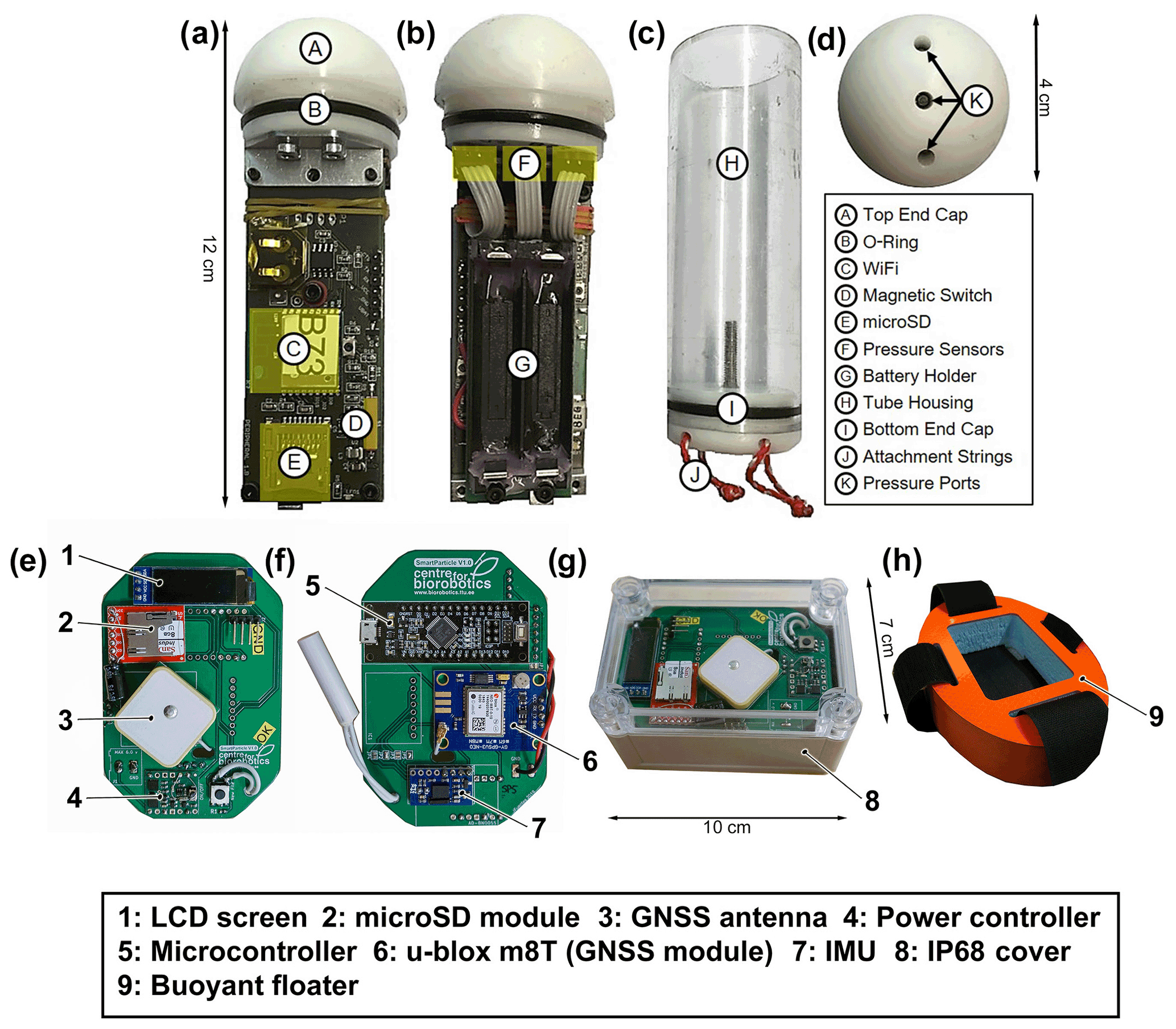
Figure 1 Two different drifter platforms have been used in this study: a submersible drifter (a–d) and a GNSS surface drifter (e–h). (a) Side view showing the submersible-drifter electronics. (b) Side view showing the reverse side of the electronics board including the battery holder and pressure sensors. (c) Polycarbonate tube housing of the submersible drifters with attachment strings for balloons used for manual buoyancy adjustment. (d) Top view facing the cap, showing the ports for each of the three pressure sensors. (e) Side view showing the GNSS surface drifter electronics with an LCD screen, microSD storage, a GNSS antenna and a power controller. (f) Side view showing the reverse side of the GNSS surface drifter electronics with a microcontroller, GNSS receiver and IMU. (g) The electronics of the GNSS surface drifter are sealed in a waterproof box. (h) The box gets placed at the center of a 20 cm long float.

2.2 Study site and fieldwork

The fieldwork was conducted in July 2019 on Austre Brøggerbreen, an approximately 5 km long valley glacier located on the Svalbard archipelago (Fig. 2). The glacier is entirely cold-based and thus characterized by low annual flow velocities (Hagen and Sætrang, 1991). Several persistent englacial channels exist on Austre Brøggerbreen, and they have been studied regularly over the past 20 years (Vatne, 2001; Stuart et al., 2003; Vatne and Irvine-Fynn, 2016; Kamintzis et al., 2018).

Our fieldwork focused on the lower englacial channel (Fig. 2c), which was mapped 20 years earlier and described by Vatne (2001) and Stuart et al. (2003). An additional lidar (laser imaging, detection and ranging) survey of parts of the channel was conducted in 2017 (Kamintzis et al., 2019). The channel is located close to the glacier snout, which is subject to rapid downwasting. As a result the channel was close to the glacier surface in 2019 and completely melted out in 2020, compared to a depth within the ice of approximately 50 m in 1999 (Vatne, 2001; Stuart et al., 2003). A small supraglacial channel further upstream of the glacier was utilized for GNSS validation (Fig. 2c).

In order to test and validate our reconstruction algorithms, both drifter platforms were deployed in the small supraglacial channel on 2 July 2019 between 12:00–18:00. Both platforms were then deployed into the englacial channel via a former moulin (Fig. 2) on 5 July 2019 between 12:00–18:00, during the period of the main spring snowmelt. All drifters were recovered by hand from a river in the glacier forefield. We revisited the englacial channel on 19 August 2020 and deployed a GNSS-enabled surface drifter to gather GNSS data from the water flow path of the now-melted-out channel. The canyon and the river in the glacier forefield were manually digitized from an optical Planet Labs satellite image (Team Planet, 2017) from 9 July 2019 using QGIS software (QGIS Development Team, 2009). Table 1 summarizes the reconstruction cases, validation methods and the number of drifter deployments for each experiment.

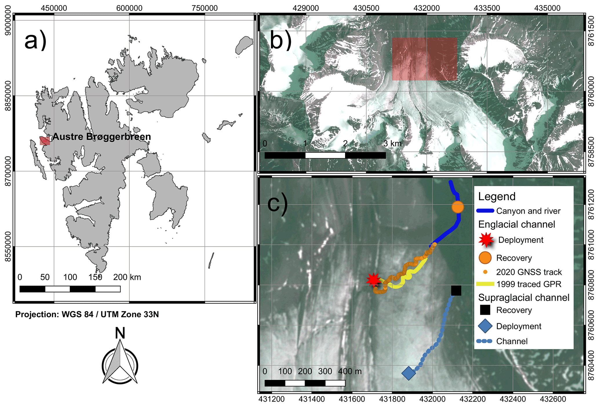
Figure 2 The test site. (a) Location of Austre Brøggerbreen on the Svalbard archipelago. (b) Location of the investigated supra- and englacial channel on the glacier. Background image: Planet Labs, 9 July 2019 (Team Planet, 2017). (c) Map of the studied supra- and englacial channel. Shown are the 2019 GNSS track with the deployment and recovery point for the supraglacial channel, the 1999 GPR track of the englacial channel from Stuart et al. (2003), and the 2020 GNSS track of the melted-out englacial channel, as well as a river and canyon section following the englacial channel, mapped out from Planet optical imagery (Team Planet, 2017). Additionally shown are the deployment and recovery points used for drifter deployments at the englacial channel. Background image: Planet Labs, 9 July 2019 (Team Planet, 2017).

Table 1 Overview of the reconstruction cases, the validation methods and the number of submersible-drifter deployments as well as the number of complete submersible-drifter datasets (i.e., the datasets that did not have any missing data and where the deployment and recovery point could be identified).

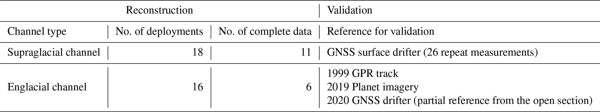
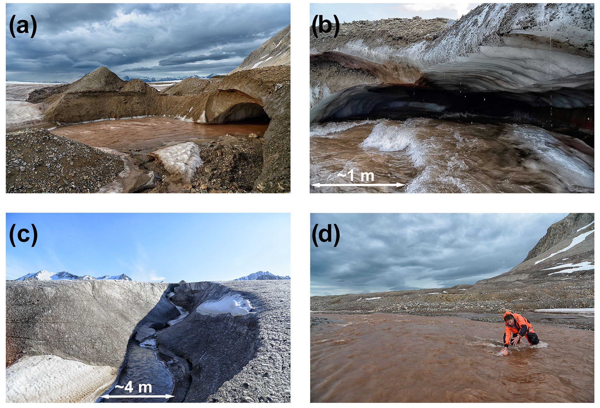
Figure 3 Pictures from the field deployments in July 2019 with approximate scale. (a) Deployment point at the englacial channel. (b) Entrance to the englacial channel. (c) Canyon following the outlet of the englacial channel. (d) Drifter recovery at the proglacial river. Images: Andreas Alexander.

2.3 Model description

The general workflow of our subsurface water flow path reconstruction is shown in Fig. 4. The input data for the noise removal and feature extraction phases are the gyroscope, acceleration and magnetometer readings of the submersible drifter's IMU. The IMUs used provide internally calculated quaternions (Zhang, 1997) as well as Euler angles (Diebel, 2006), providing information about the device orientation. The output of the model is the average 2D water flow path in UTM coordinates (WGS 84, UTM zone 32N; World Geodetic System, Universal Transverse Mercator) with pressure distribution.

For channel reconstruction, additional input is needed to specify the start and end points of the water flow path. In our case, those are GNSS referenced deployment and recovery coordinates of the drifters. The processing and modeling of drifter data from one deployment took on average 20 min. For this, we used MATLAB 2019b software on a consumer laptop (1.8 GHz Intel Core i7, 8 GB RAM).

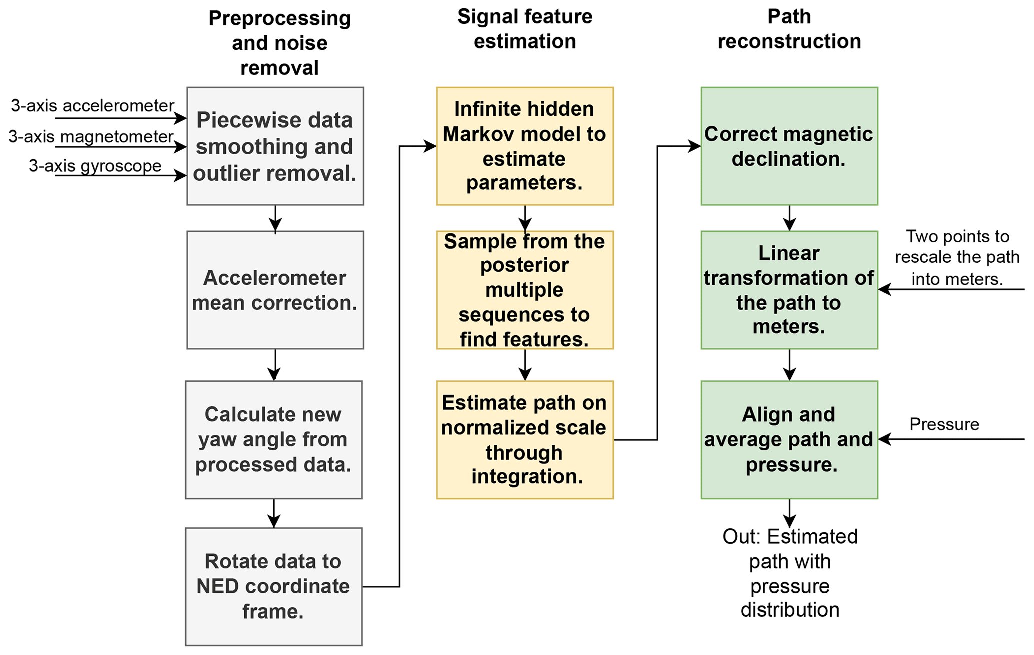
Figure 4 Workflow diagram of the processing sequence. The model applies an infinite hidden Markov model (iHMM; see Beal et al., 2002) on the IMU data to detect signal features. NED stands for north–east–down.

2.4 Preprocessing and noise removal

The data from each submersible-drifter deployment were manually clipped to consider only the time between deployment and recovery. Each deployment resulted in a separate independent dataset, used for water flow path reconstruction. Every dataset consisted of IMU sensor data with 9 degrees of freedom (three-axis accelerometer, three-axis magnetometer and three-axis gyroscope) at 100 Hz and readings from three pressure sensor readings.

In order to obtain an accurate orientation estimation, the IMU data were piecewise filtered; the outliers were removed; and a mean correction was applied to the accelerometer data. For this, the data were split up where the mean of the signals changed significantly (Killick et al., 2012). The subdivision of the data was followed by removing noise from each section separately, in order to avoid over-smoothing of the remaining water flow path. A first-order Savitzky–Golay filter (Savitzky and Golay, 1964) was then applied to both accelerometer and magnetometer data in each section to remove high-frequency noise. This filter was chosen, as it preserved high-frequency signal components better than other commonly used filters. Afterwards, outliers were manually removed using a variance-based outlier filter with a 1σ threshold if the standard deviation of the selection was over 3 and 2σ when below. Abrupt changes in the acceleration behavior led to significant errors in the rotation calculation and hence considerable jumps in the reconstructed water flow path. To smooth these jumps, we applied a componentwise mean correction on the accelerometer data. For this, we calculated the mean along the whole water flow path and each individual section. We then computed the average between the total water flow path mean and each section mean and set this average as the new mean for each section.

The data were rotated into a Cartesian north–east–down (NED) coordinate system, using the pitch and roll angles from the device and the yaw angle calculated from the processed accelerometer and magnetometer readings. As the computational complexity of the data processing is non-linear, the data were downsampled from 100 to 25 Hz by decimating the signal by a factor of 4 to increase the model's processing speed.

2.4.1 Estimating the signal features using an infinite hidden Markov model

Hidden Markov models (HMMs) are unsupervised learning models in which the state is not fully observable; instead it is observed indirectly via noisy observations (Rabiner and Juang, 1986). In this study, the noisy observations are the IMU-derived accelerometer, magnetometer and gyroscope signals. Using an HMM, we find hidden states (or features), which we assume to be associated with velocity changes. That is, we assume that at the beginning of each hidden state, the componentwise velocity is zero (or close to zero). Therefore, similarly to Fourati et al. (2013), using gait to avoid integration errors growing unbounded, we will be making use out of salient flow features.

First, consider a finite (regular) HMM that takes the measured IMU time series data, denoted by $\mathit{y}=\mathit{\{}{y}_{\mathrm{1}},y_{\mathrm{2}},\mathrm{\dots },y_T\mathit{\}}$ as input (observation sequence), and finds the hidden state sequence $\mathit{s}=\mathit{\{}{s}_{\mathrm{1}},s_{\mathrm{2}},\mathrm{\dots },s_T\mathit{\}}$, which, in the scope of this paper, is assumed to be the velocity features of the water flow in the channel (e.g., step-pool sequences, meander bends). In finite HMMs, each state takes a value from a finite number of states $\mathrm{1},\mathrm{\dots },K$, which have to be predefined. A transition matrix π describes the probabilities of moving between states. The probability of moving from state i at time t to state j at time t+1 is given as ${\mathit{\pi }}_{ij}=p(s_t=i\mid s_{t+\mathrm{1}}=j)$, and the initial probabilities are given by ${\mathit{\pi }}_{\mathrm{0}i}=p(s_{\mathrm{1}}=i)$. In addition, there exists a quantity ${\mathit{\varphi }}_{s_t}$ for each state $s_t\in \mathit{\{}\mathrm{1},\mathrm{\dots },K\mathit{\}}$ that parameterizes the observation likelihood for that state given by $y_t\mid s_t\sim F\left({\mathit{\varphi }}_{s_t}\right)$. The observation likelihood describes the probability of an observation y_t being generated from a state. Hence, the HMM can be written as $\mathit{\{}{\mathit{\pi }}_{\mathrm{0}},\mathit{\pi },\mathit{\varphi },K\mathit{\}}$. The joint distribution over hidden states s and observations y, given the parameters $\mathit{\{}{\mathit{\pi }}_{\mathrm{0}},\mathit{\pi },\mathit{\varphi },K\mathit{\}}$, can be written as

$$\begin{array}{}\text{(1)}& p(\mathit{s},\mathit{y}\mid {\mathit{\pi }}_{\mathrm{0}},\mathit{\pi },\mathit{\varphi },K)=\prod _{t=\mathrm{1}}^{T}p(s_t\mid s_{t+\mathrm{1}})p(y_t\mid s_t).\end{array}$$

The finite HMMs have two limitations: first, maximum likelihood estimations do not consider the complexity of the model. This makes underfitting and overfitting hard to avoid. Second, the model has to be specified in advance. This means that even though the hidden states are unknown, the number of different states has to be predefined. Due to the complexity of the model, predefining it is difficult, as one has to choose the number of different features in the glacial channels based only on the measured IMU data. Hence, a more computationally expensive but more flexible infinite hidden Markov model (iHMM) (Beal et al., 2002) will be used to address these limitations.

The iHMM uses Dirichlet processes to define a non-parametric Bayesian analysis on an HMM, allowing a countably infinite number of hidden states, thus permitting automatic determination of the number of hidden states. Therefore, not knowing how many different features are present in the glacial channel is not a problem anymore. In an HMM, the transition matrix π is a K×K matrix, where K is predefined. In iHMM, by contrast K→∞. To allow this and to complete the Bayesian description, the priors are defined using hierarchical Dirichlet processes (HDPs), allowing for distributions over hyperparameters and making the model more flexible.

The HDPs are a set of Dirichlet processes (DPs) coupled through a shared random base measure drawn from a DP. That is, each $G_k\sim \mathrm{DP}(\mathit{\alpha },G_{\mathrm{0}})$ with a shared base measure G₀ and a concentration parameter α>0. The shared base measure can be thought of as the mean of G_k, and the concentration parameter α controls the variability around G₀. In addition, the shared base measure is also given a DP prior $G_{\mathrm{0}}\sim \mathrm{DP}(\mathit{\gamma },H)$, where H is a global base measure. The formal definition of the iHMM is given as

$$\begin{array}{}\text{(2)}& {\displaystyle }\mathit{\beta }& {\displaystyle }\sim \mathrm{GEM}\left(\mathit{\gamma }\right)\text{(3)}& {\displaystyle }{\mathit{\pi }}_k\mid \mathit{\beta }& {\displaystyle }\sim \mathrm{DP}(\mathit{\alpha },\mathit{\beta })\text{(4)}& {\displaystyle }{\mathit{\varphi }}_k& {\displaystyle }\sim H\text{(5)}& {\displaystyle }{s}_t\mid s_{t-\mathrm{1}}& {\displaystyle }\sim \mathrm{Multinomial}\left({\mathit{\pi }}_{s_{t-\mathrm{1}}}\right)\text{(6)}& {\displaystyle }{y}_t\mid s_t& {\displaystyle }\sim F\left({\mathit{\varphi }}_{s_t}\right),\end{array}$$

where DP(α,β) is a DP and the parameter β is a hyperparameter for the DP that is distributed according to the stick-breaking construction noted as Griffiths, Engen and McCloskey's distribution GEM(.) (Sethuraman, 1994). The indicator variable s_t is sampled from the multinomial distribution, and $F\left({\mathit{\varphi }}_{s_t}\right)$, for the purpose of this paper, is assumed to be a normal distribution. Finally, priors are also put on hyperparameters α and γ. As there are no strong beliefs about the hyperparameters, a common practice is to use gamma hyperpriors.

To find the two sets of unknowns, i.e., the hidden states and the hyperparameters, beam sampling (Van Gael et al., 2008; Van Gael, 2009) is used. The beam sampling combines slice sampling and dynamic programming, where the first limits the number of states considered at each time step to a finite number and the second samples the hidden states efficiently.

2.4.2 Water flow path reconstruction

The model proposed gives a posterior probability over sequences of observations that have been found, and multiple possible velocity feature (hidden state) sequences are sampled from the posterior distribution. This results in a set of possible sequences of flow features along the glacial-water flow path. Therefore, the reconstructions are performed for multiple feature sequences, hence creating multiple possible water flow paths and an estimated region of error.

To get the estimated water flow path via dead reckoning, the accelerometer data are integrated twice over time. To get a more accurate estimation, the features from an iHMM are used, and the integration is done over the features separately. The integration is done in two steps. Assuming that the componentwise velocity is zero at the beginning of each feature, the first integration is calculated over each feature separately, setting the component velocity to zero at the beginning. This results in a velocity profile that does not correspond to the real velocity values along the water flow path; however, it describes the changes in velocity along the water flow path. The second integration is performed over the new velocity profile and normalized, resulting in the glacier water flow path on a normalized scale. After correcting for magnetic declination, using the MATLAB inbuilt function (https://uk.mathworks.com/help/aerotbx/ug/igrfmagm.html, last access: 19 October 2021) for calculating Earth's magnetic field using the International Geomagnetic Reference Field (Blakely, 1996; Lowes, 2010), the resulting topology map is rescaled to Earth coordinates through a linear transformation. This transformation can be found by knowing two distinct points along the water flow path, in our case, the deployment and recovery positions. The reconstructed water flow paths from each deployment and their pressure distributions are aligned and averaged. The alignment was performed using dynamic time warping (Sakoe and Chiba, 1978) such that each subsequent signal was aligned with the mean of previous signals. The result is an estimated water flow path which can be used to spatially reference the pressure distribution in 2D.

3 Results

3.1 Supraglacial reconstruction and validation

The method using submersible sensing drifters and data processing proposed in this paper was used in reconstruction of a supraglacial channel (Fig. 5a) with known geometry (Fig. 2c). As a reference, we used an averaged water flow path (Table 1), derived from GNSS surface drifter measurements along the supraglacial channel. The final averaged water flow path was based on the 26 independent repeat measurements along the supraglacial channel. The difference between the average GNSS measured water flow path and the individual GNSS drifter measurements had a mean of 3.5 m and standard deviation of 5.5 m. We calculated the position error for each point on the reconstructed water flow path as

$$\begin{array}{}\text{(7)}& \text{Error}=\sqrt{\left(p_x\right(t)-{\widehat{p}}_x(t){)}^{\mathrm{2}}+(p_y\left(t\right)-{\widehat{p}}_y\left(t\right){)}^{\mathrm{2}}},\end{array}$$

where p_x(t) and p_y(t) are the coordinates measured via GNSS and ${\widehat{p}}_x$ and ${\widehat{p}}_y$ are the estimated points from the reconstruction. The reconstruction was based on 11 submersible-drifter deployments. Our model reproduces a water flow path, which is on average within 3.9 m of the GNSS reference channel (Fig. 5). The lowest position error is 2.0 m, and the most significant deviation from the reference water flow path is 11.1 m, based on the average of the 10 nearest points. As Fig. 6 shows, the average position error from our reconstruction converges after six datasets (one drifter deployment needed per dataset). The total length of the GNSS reference track is 449 m, whereas the reconstructed water flow path is 478 m long, hence resulting in an overestimation of 6.5 %. The resulting water flow path allows for referencing the pressure measurements of the drifters spatially. The resulting pressure distribution map shows the pressure variations along the channel (Fig. 5c). Zones of higher pressures occurred mainly in the lower part of the channel, as the drifters moved from a higher elevation down to lower elevation and in areas where the channel changes direction.

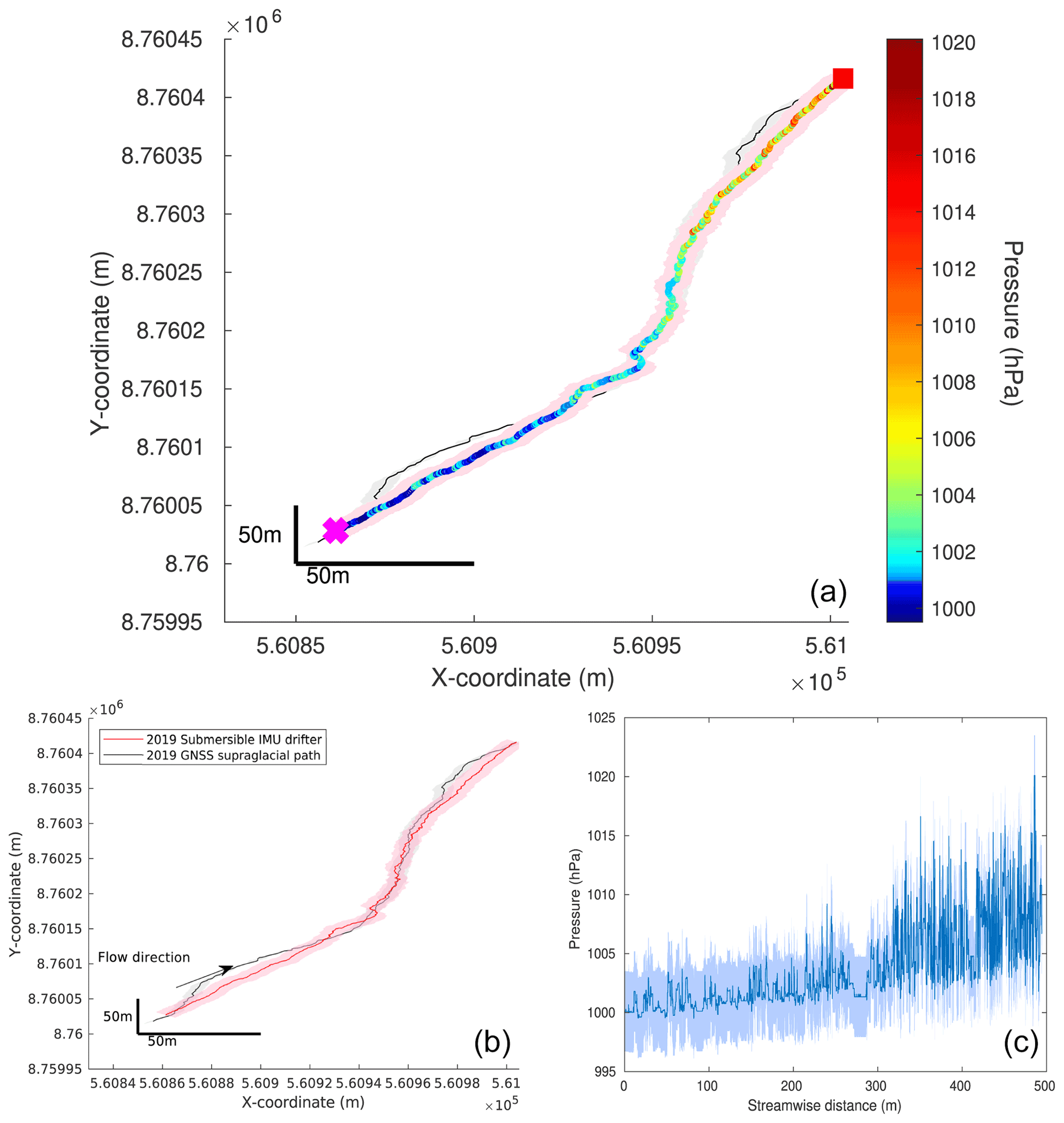
Figure 5 Supraglacial-water flow path reconstruction. (a) Reconstructed supraglacial track in UTM coordinates with pressure distribution in hectopascals. The deployment is marked with a pink cross, and the recovery is a red square. (b) Estimation of the supraglacial track (red) with standard deviations (pink) in UTM coordinates. The GNSS reference is shown in black, and the average error of the GNSS recordings is in light gray. (c) Average water pressure with standard deviation along the estimated streamwise distance of the supraglacial channel.

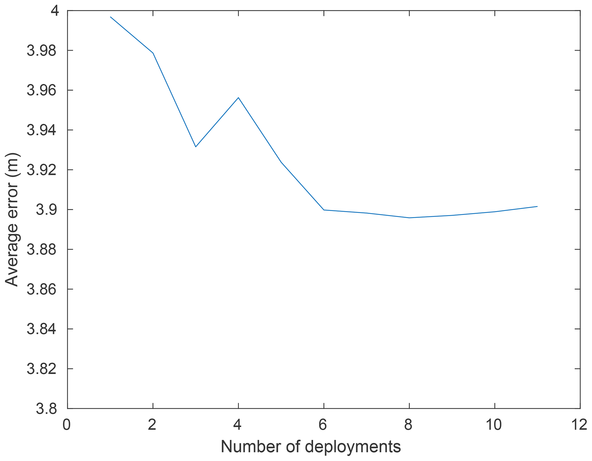
Figure 6 Convergence of the average error for the supraglacial channel reconstruction with respect to the number of deployments. Each deployment results in a separate independent dataset that is used to create a new distinct water flow path reconstruction. The reconstructed water flow paths are aligned and averaged.

3.2 Englacial channel reconstruction and validation

The submersible-drifter deployments for the water flow path reconstruction (Fig. 7a) were conducted in July 2019. A revisit of the field site in August 2020 allowed us to map the water flow path of the channel with the GNSS surface drifter, as the roof of the channel had mostly melted away and transformed the former englacial channel into a deeply incised supraglacial channel, which was only partly ice-covered. The reconstruction from the IMU data, collected in 2019 (six datasets), leads to the mean water flow path shown in Fig. 7b. The figure also shows the comparison between a GNSS reference track measured 1 year later in summer 2020 and a GPR measurement from 1999. There are clear similarities between the shape of the reconstructed water flow path and the shape of both the 2020 GNSS reference and the 1999 GPR track from Stuart et al. (2003).

The average position error (based on Eq. 7) of the reconstructed englacial channel and the proglacial river, compared to the 2020 GNSS reference path for the channel, as well as the 2019 satellite-derived proglacial river path (Fig. 7), is 12.1 m. The englacial channel part of the reconstruction has an average position error of 13.3 m compared to the 2020 GNSS reference (Table 1 for an overview of used references). From the englacial outlet through the canyon (Fig. 3c) and the proglacial river up to the recovery point (Fig. 3d), the average position error of the reconstructed water flow path is 10.9 m compared to the satellite reference. The 2020 GNSS reference track (one deployment) from the englacial channel has a length of 545 m. The section after the outlet of the channel through the canyon and the proglacial river measures 290 m on the satellite imagery. Our model returns a total channel length of 1027 m from the deployment point to the recovery point, where the channel section is 651 m long and the part through the canyon and the proglacial river is 376 m.

The mean pressure recorded by the drifters is 1011.7 hPa with a standard deviation of the time series data of 3.4 hPa (0.3 %). The spatial-pressure-distribution map (Fig. 7a) reveals one zone of higher pressure shortly before the englacial channel exits into the open canyon (black square in Fig. 7a). The average water pressure of multiple deployments reaches up to 1070 hPa, compared to maximum values of 1300 hPa recorded by the individual submersible drifters before averaging.

The water flow path of the englacial channel, investigated in this study, has been repeatedly mapped by previous studies. These studies offer additional references to assess the feasibility of the reconstruction qualitatively. Stuart et al. (2003) utilized GPR to draw a map of the channel (shown in Fig. 2c), whereas Vatne (2001) used speleological investigations, providing a very simple map in his publication.

The qualitative comparison between the 1999 GPR reconstruction of the englacial channel from Stuart et al. (2003) and our GNSS surface drifter measurements from 2020 shows good accordance in the overall shape of the water flow path in Fig. 7b. It is also visible in Fig. 7b that the channel developed by both vertical and lateral incision, keeping its overall shape over the 21 years spanning between the two investigations. The satellite reference used for the canyon (Fig. 3c) and the proglacial river (Fig. 3d) was mapped on Planet imagery, which has a positional accuracy of less than 10 m root mean square error (Team Planet, 2017). The canyon was barely visible on the imagery leading to a straight reference track instead of a meandering one. However, the sharp turn of the river after the canyon exit is visible on the satellite imagery and can be matched to the topology of the reconstructed water flow path.

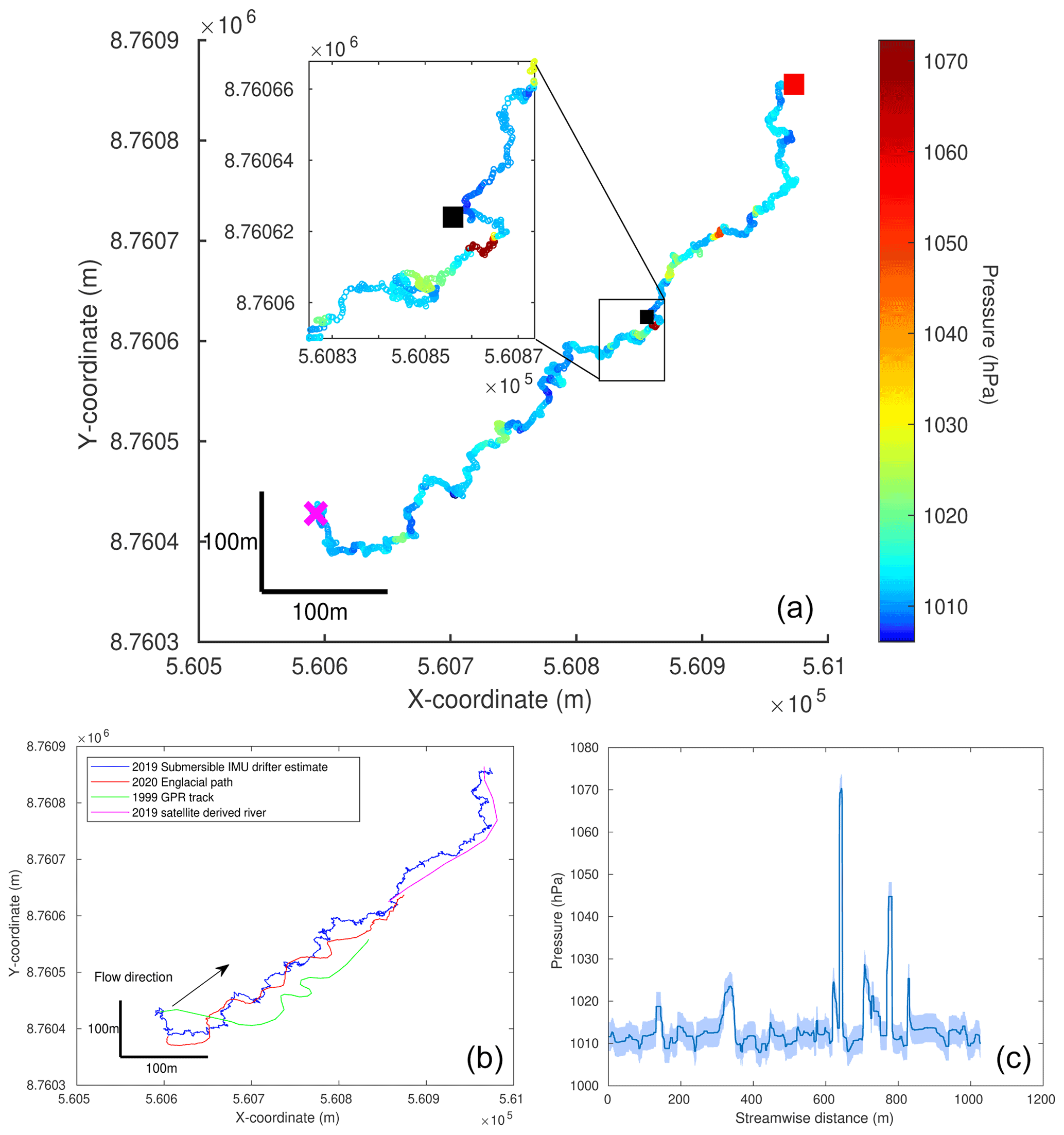
Figure 7 Englacial channel reconstruction. (a) Estimated average track of the englacial channel in UTM coordinates with pressure distribution in hectopascals. The deployment is marked with a pink cross, and the recovery is a red square. Additionally shown is the location of the start of the canyon at the end of the englacial channel (black square). (b) Estimated englacial track in UTM coordinates based on the 2019 IMU data in blue alongside a GNSS drifter reference measured in 2020 in red. Further shown are the mapped canyon and proglacial river from optical Planet imagery (acquisition date: 9 July 2019; Team Planet, 2017), as well as the 1999 GPR map traced from Stuart et al. (2003). (c) Average water pressure with standard deviation along the estimated streamwise distance of the englacial channel.

4 Discussion

We present the topological reconstruction of a supra- and englacial channel on Austre Brøggerbreen (Svalbard). The motivation for this study was to provide in situ measurements from englacial channels and to show that it is possible to map glacier water flow paths using submersible drifters. The contribution of this paper is a method for mapping subsurface flows using submersible drifters' IMU measurements and mapping the pressure readings of the sensors along the reconstructed water flow path. The comparison with GNSS tracks (at open parts of the channels), as well as to the previous studies of the same englacial channel at Austre Brøggerbreen, provided quantitative and qualitative reference.

4.1 Comparison to GNSS measurements

The reconstructed water flow paths were compared to the GNSS measurements at the open parts of the channels and revealed the average error in the length estimate of 6.5 % for the supraglacial and 11.6 % for the englacial channel. The accuracy of the used GNSS reference is, however, limited. The static positioning error of the used GNSS receivers is ±3 m, with the dynamic positioning error, in a highly turbulent supraglacial stream, certainly being much higher. The used GNSS reference is additionally an aligned average of 26 single tracks, over-smoothing several meander bends and therefore smoothing the real channel geometry. An average error of 3.9 m for the reconstruction versus the GNSS reference is therefore likely below the accuracy of the GNSS reference track itself.

The water flow path length of the englacial reconstruction is 1027 m, much longer than the sum of the GNSS and the satellite reference of 835 m. However, the GNSS reference is missing the first section of the englacial channel after deployment due to changed water pathways between 2019 and 2020. Based on handheld GPS measurements (±5 m) plotted within QGIS, this length difference is estimated to be 85 m. This leaves a difference of 107 m between reference water flow path length and the reconstruction or an overestimation of the water flow path by 11.6 %. This does not take into account that the satellite reference is underestimating the real water flow path length. Therefore, the real length error of our reconstruction is likely much lower. On the other hand, the drifter-based reconstruction could also overestimate the channel length. Our reconstruction is based on the distance traveled by the drifters. As they can get stuck in eddies or travel from one side of the channel to the other, the reconstructed water flow path becomes longer than the real channel. This can also be seen in very wobbly sections of the channel reconstruction in Fig. 7a.

The hydrological system of Austre Brøggerbreen has been studied several times in the past and thus offers the possibility of evaluating the feasibility of our reconstruction. We have shown that some prominent features (large bends and step-pool sequences) reoccur between our reconstruction and previous studies. Glacier drainage systems do, however, evolve throughout different seasons (e.g., Church et al., 2020) and can therefore change over time. It is therefore difficult to establish if the discrepancies between our reconstruction and previous studies are due to an inaccurate reconstruction or can be attributed to the changes of the channel itself. Assuming the later would offer the opportunity to study the evolution of an englacial channel over a several-decade-long time span.

4.2 Pressure data

The pressures recorded by the submersible drifters in the englacial channel show flow under atmospheric conditions. Pressurized flow conditions, with water flowing partly uphill as encountered by Stuart et al. (2003), no longer exist within the channel. The average standard deviation of the pressure data is, with 3.4 hPa, similar to our previous work (Alexander et al., 2020a), thus very low. It is most likely influenced by the pressure variability within the channel rather than the accuracy of the pressure sensor. Within the englacial channel itself, one zone of abrupt and high-pressure change exists shortly before the channel exits into the canyon. Similar to pressure peaks studied in Alexander et al. (2020a), we interpret this as the presence of a step-pool sequence with a large step riser. This interpretation was confirmed by speleological investigations in 2018, where a roughly 2.5 m high step riser was found at the same location. The step can also be seen in the lidar scans from Kamintzis et al. (2019). This shows that our method allows for identifying and locating step-pool sequences within glacial channels. This is of relevance, as step-pool sequences feature locally enhanced erosion and are therefore discussed as a mechanism by which supraglacial channels can incise into ice and transform into englacial channels (Gulley et al., 2009; Vatne and Irvine-Fynn, 2016). Step-pool sequences are further thought to account for a large part of the hydraulic roughness encountered within a channel (Vatne and Irvine-Fynn, 2016) and can account for up to 80 % of the change in channel elevation (Vatne, 2001). Being able to correctly identify and spatially locate steps in the subsurface could therefore contribute towards an enhanced understanding of the water transit from the ice surface through the englacial system all the way to the glacier bed, especially if measurements are successfully repeated over multi-year periods.

4.3 Number of deployments

In this study, we used a relatively low number of deployments (11 for the supraglacial channel and 6 for the englacial channel) for the reconstruction with an average error of 3.9 and 12.1 m, respectively. The average error calculations for the supraglacial channel (Fig. 6) show that the error converges at six deployments. The decrease in the average error with increasing deployment number is, however, so low (2.5 %) that a single deployment would already lead to sufficient precision. Using the values for the mean pressure and its standard deviation leads to a precision of 0.66 % with just one deployment, according to Eq. (4) in Alexander et al. (2020a). This shows that our approach can produce a highly precise topological reconstruction and spatial pressure distribution from just one deployment. As we have lost one submersible drifter out of 16 deployments at the englacial channel (93.8 % recovery rate) and encountered technical problems (e.g., drifter switched off during deployment, damaged pressure recordings) with quite some of the retrieved datasets (utility rate of only 40 %), we estimate that at least 3 submersible-drifter deployments will be needed in the field in order to obtain the topology of a 1 km long englacial channel. These numbers are, however, likely to scale with increasing channel lengths as experience from Bagshaw et al. (2012) shows, where the recovery rate of retrieved drifters decreased with increasing distance of the deployment point from the glacier margin.

4.4 Comparison with GPR, perspectives and limitations

Of special interest within glaciology is also the comparison of our method with the currently most commonly used method to localize glacial drainage systems: GPR. Most recently Church et al. (2020) reconstructed an englacial channel on Rhonegletscher in Switzerland, both in 2D (Church et al., 2020) and in 3D (Church et al., 2021). In their 2020 study, Church et al. (2020) reported a length error of 2.4 % (6 m) for a 250 m long englacial channel. Our method showed a length error of 6.5 % for a 500 m long supraglacial channel and 11.6 % for a 1 km englacial channel. This indicates that the error in our method scales with the length of the investigated channel, thus resulting in a similar length error as reported for the GPR investigations by Church et al. (2020) if scaled down to similar shorter channel length. However, our method only allows for reconstructing the actual water flow path and can currently not be used to infer information about channel width and height, as is possible with GPR (e.g., Stuart et al., 2003; Church et al., 2020, 2021). The application of our drifter-based approach, in comparison to GPR, is further limited by a certain minimum needed discharge in combination with sufficient drainage system size for drifters to pass through, thus limiting the applicability to the main part of the melt season and channelized drainage systems. Another limitation of the drifter-based approach is the battery lifetime of the drifters (currently around 10 h for the submersible drifters), thus limiting it to channels where the water transit takes less than the expected battery lifetime. The main shortcoming of our current drifter-based approach is the need for instrument recovery. Given the scale of many glacial systems, the comparatively tiny size of the drifters and the harsh conditions encountered at glacial outlets (e.g., strong flowing rivers, calving fronts), recovery poses a major challenge. In the future this might be overcome by adding localization devices to the drivers and utilizing autonomous platforms (e.g., drones, boats) for instrument recovery, as well as enabling data communication while the instruments are still within the ice to remove the necessity of their recovery. Deliberate choice of field site (e.g., lake-terminating glaciers, subglacial laboratory) might further help in this endeavor.

At the current stage, we are only able to produce the planar topology of the water flow path. A full 3D reconstruction, comparable to results achieved via GPR (Church et al., 2021), was not possible, as the IMUs did not correct for the gravity vector. Removing the gravity vector in the postprocessing stage introduces additional uncertainty and therefore renders an inaccurate elevation track. We are, however, optimistic that we will be able to do full 3D reconstructions in an improved version of our method by collecting additional vertical reference data and accounting for the error introduced by the gravity vector. The general difficulty with the validation of IMU data (e.g., due to accelerometer gravity compensation, dead-reckoning error) has also been noted by Maniatis (2021) as a general problem within geomorphological IMU applications, as common standards have not been formulated yet. At the current stage our model is also not able to calculate the numerical velocity, as the model operates largely on a normalized space. Another development step will therefore be to reconstruct flow velocities utilizing the timestamp of the IMU recordings alongside the reconstructed water flow path length.

Besides the shortcomings, our method also offers several advantages compared to traditional GPR investigations. First of all the method allows for directly measuring spatially referenced pressure conditions in the subsurface, thereby having a great advantage compared to other methods where the pressure can only, if at all, be derived indirectly using geophysical models. Adding additional sensor payloads to the drifter or replacing the current 2 bar pressure sensors with 30 bar sensors would further allow for gaining additional spatially referenced physical information about the glacial drainage system and, in cases where successful recovery is possible, also from the subglacial system. Church et al. (2020, 2021) name two main disadvantages of GPR systems. The first is the exposition to risky areas of the glacier surface while conducting measurements (Church et al., 2020). In case of drifters this need is greatly limited, as only a single deployment point is needed (compared to kilometer long transect lines), and the utilization of drones and other aerial vehicles for drifter deployment could completely eliminate the need for personnel to access the glacier surface. The second point is the time-consuming nature of GPR investigations, often on the order of several days (e.g., 9 d in Church et al., 2021). In the case of our approach, this time and thus the associated costs can be greatly reduced, as it took on average 11 min per drifter to pass the approx. 1 km long channel.

Most likely the strength of our method will lie in a combination with other approaches. It is for example possible that drifters could deliver information about the nature of reflectors in GPR signals, while GPR is utilized in areas too small for drifters to pass through or in locations where recovery is unlikely. At the same time drifters will be able to supplement valuable in situ data from GPR investigated channel geometries and extend their measurements to areas currently not covered (e.g., heavily crevassed). Similarly, the drifters could be used to collect complementary information to seismic arrays. In Nanni et al. (2021), the authors state that the method using seismic array would benefit from complementary in situ observations. The drifter measurements could provide data to inform the best placements of seismic arrays and provide in situ pressure measurements. The affordability and simple-to-use nature of the proposed sensing drifter platforms allows for widening the usage of the proposed method. Further, the relatively small scale of the drifters would make it easy to include as a complementary measure at field tests. We are therefore overall positive that our method, given further developments, will be of great value to the glaciological community in the near future.

5 Conclusions

In this paper, a method allowing in situ repeat measurements from subsurface water flow paths is presented along with a model to reconstruct the water flow paths from these data. The method is applied to a free-flowing englacial channel on Svalbard to showcase its feasibility to collect spatially referenced in situ measurements from glacial channels.

The main focus of our presented method is to provide spatial reference for measurements where such reference is currently lacking. This is due to the underground nature of many water flow environments preventing the application of GNSS technology for localization. Our proposed method utilizes infinite hidden Markov models and shows the possibility of reconstructing water flow paths from inertial data with only two given coordinates. We apply this to the study of an englacial channel and show that we could reconstruct the geometry of the channel from just one submersible-drifter dataset on a consumer laptop. This implies that our method might be upscalable and could open up for interesting studies investigating water transits through glaciers with in situ data. It is further feasible to apply this method to other applications where repeat measurements from hazardous and hard-to-access water flow measurements are required. This suggests that our results might have significant future implications, not only within glaciology but also for subsurface flow studies in general.