Review article: Global monitoring of snow water equivalent using high-frequency radar remote sensing

Seasonal snow cover is the largest single component of the cryosphere in areal extent, covering an average of 46 × 10⁶ km² of Earth's surface (31 % of the land area) each year, and is thus an important expression and driver of the Earth's climate. In recent years, Northern Hemisphere spring snow cover has been declining at about the same rate (∼ −13 % per decade) as Arctic summer sea ice. More than one-sixth of the world's population relies on seasonal snowpack and glaciers for a water supply that is likely to decrease this century. Snow is also a critical component of Earth's cold regions' ecosystems, in which wildlife, vegetation, and snow are strongly interconnected. Snow water equivalent (SWE) describes the quantity of water stored as snow on the land surface and is of fundamental importance to water, energy, and geochemical cycles. Quality global SWE estimates are lacking. Given the vast seasonal extent combined with the spatially variable nature of snow distribution at regional and local scales, surface observations are not able to provide sufficient SWE information. Satellite observations presently cannot provide SWE information at the spatial and temporal resolutions required to address science and high-socio-economic-value applications such as water resource management and streamflow forecasting. In this paper, we review the potential contribution of X- and Ku-band synthetic aperture radar (SAR) for global monitoring of SWE. SAR can image the surface during both day and night regardless of cloud cover, allowing high-frequency revisit at high spatial resolution as demonstrated by missions such as Sentinel-1. The physical basis for estimating SWE from X- and Ku-band radar measurements at local scales is volume scattering by millimeter-scale snow grains. Inference of global snow properties from SAR requires an interdisciplinary approach based on field observations of snow microstructure, physical snow modeling, electromagnetic theory, and retrieval strategies over a range of scales. New field measurement capabilities have enabled significant advances in understanding snow microstructure such as grain size, density, and layering. We describe radar interactions with snow-covered landscapes, the small but rapidly growing number of field datasets used to evaluate retrieval algorithms, the characterization of snowpack properties using radar measurements, and the refinement of retrieval algorithms via synergy with other microwave remote sensing approaches. This review serves to inform the broader snow research, monitoring, and application communities on progress made in recent decades and sets the stage for a new era in SWE remote sensing from SAR measurements.

1 Introduction

Seasonal snow on land is responsible for a number of important processes and feedbacks that affect the global climate system, fresh water availability to billions of people, biogeochemical activity including exchanges of carbon dioxide and trace gases, and ecosystem services. Despite this importance, snow mass (commonly expressed as the snow water equivalent, or SWE) is a poorly observed component of the global water cycle. Given the vast area of Northern Hemisphere snow extent (exceeding 45 × 10⁶ km² each winter), surface observing networks are insufficient as a sole source of information for snow monitoring. Satellite remote sensing is the only means to monitor SWE consistently and continuously at continental scales. Optical satellite imagery acquired under cloud-free conditions can provide information on where and when snow is on the ground but does not support the retrieval of SWE. Long time series of snow mass information are available from satellite passive microwave measurements (Luojus et al., 2021), but at coarse spatial resolution (gridded at 25 km spatial resolution), mountain areas across which high values of SWE occur are excluded, and bias correction is required under deep-snow conditions (>150 mm SWE; Pulliainen et al., 2020). Land surface models driven by meteorology from atmospheric reanalysis can produce hemispheric-scale SWE information at coarse spatial resolutions (e.g., Kim et al., 2021), but there is a large spread between products due to differences in the meteorological forcing data (especially precipitation) and a pronounced negative bias in mountain areas (Wrzesien et al., 2019a; Cao and Barros, 2020; Lundquist et al., 2019). Differential airborne and ground-based lidar altimetry (Deems et al., 2013; Meyer et al., 2021) and spaceborne stereo photogrammetry (Deschamps-Berger et al., 2020) can provide snow depth information at high resolution by differencing repeat digital elevation models but are limited to small spatial domains and sparse temporal sampling. C-band radar has recently been applied to retrieve snow depth in mountainous regions (Lievens et al., 2019) using empirical relationships derived from ground-based measurements; however, this approach is not demonstrated for the comparatively shallow snowpack found across large regions of the Northern Hemisphere. Airborne and tower-based measurements have also identified the possibility of retrieving snow parameters from L-band interferometric synthetic aperture radar (SAR; Deeb et al., 2011); P-band signals of opportunity (Shah et al., 2017; Yueh et al., 2021); wideband auto-correlation radiometry (Mousavi et al., 2019); and frequency-modulated, continuous-wave (FM–CW) radar (Yan et al., 2017).

Ku- and X-band radar measurements, in contrast, provide a viable pathway to produce SWE information at the temporal and spatial scales necessary to advance operational environmental prediction, climate monitoring, and water resource management across the Northern Hemisphere (see Sect. 2 for an overview of the scientific requirements for snow mass information). Significant progress was made over the past decade in understanding the Ku-band and X-band radar response to variations in SWE, snow microstructure, and snow wet/dry state. The ESA Cold Regions Hydrology High-Resolution Observatory (CoReH₂O) mission (dual-frequency X- and Ku-band, Phase A completed at ESA in 2013; ESA, 2012; Rott et al., 2010) was a major impetus. The potential for Ku-band radar was previously explored at NASA as part of the Snow and Cold Land Processes Mission and supporting Cold Land Processes Experiment (Yueh et al., 2009). Experimental tower and airborne measurements have been used to advance understanding of the physics of backscatter response to snow microstructure and SWE (Lemmetyinen et al., 2018; King et al., 2018), including the complicating effects of forest cover (Montmoli et al., 2016; Cohen et al., 2015). Innovative new field measurements of snow microstructure parameters (Löwe et al., 2013; Kinar and Pomeroy, 2015) now provide the quantitative observational basis for radar modeling of layered snowpacks (Tsang et al., 2018) and radar retrieval algorithms (Zhu et al., 2018). Radar forward models and potential algorithm approaches have matured over the past decade, which has allowed new retrieval pathways to emerge which build on approaches first proposed for CoReH₂O.

The purpose of this review is to summarize the status of all the components necessary to fully develop the scientific readiness for a potential future radar mission focused on seasonal snow mass. This includes the theoretical sensitivity to SWE via volume scattering processes including the influence of surface and ground contributions (Sect. 3) and approaches to SWE retrieval as supported by physical snow and radiative transfer modeling (Sect. 4). Results from previous ground, tower, and airborne measurement campaigns are also reviewed. The sensitivity of Ku-band SAR measurements to SWE are limited to a threshold of approximately 150 mm (about 1 m of snow depth depending on density) because of saturation of radar volume scattering. Thus, synergy with C-band Sentinel-1 data for snow depths beyond 1 m (Lievens et al., 2019) is also explored. Other synergies with interferometric SAR, radar tomography, passive microwave, and L- and C-band SAR measurements are also described to provide ancillary information and to improve retrieval performance (Sect. 5).

2 Scientific objectives of global remote sensing of SWE and spatial and temporal requirements

High-priority science objectives require snow mass information at moderate spatial resolution (250–500 m) and frequent revisit (∼ 3–5 d; ESA, 2012; Derksen et al., 2021), a measurement paradigm that is currently not available. As outlined below, these science requirements support applications related to climate services and operational environmental prediction including quantifying snow mass contributions to water, energy, and geochemical cycles; better prediction of spring flooding; and adaptation of cold-region water resources to climate change.

1. Inventory how much water is stored as seasonal snow and how it varies in space and time.

   The amount and distribution of and variability in terrestrial SWE across the Northern Hemisphere is poorly quantified because surface networks are inadequate, and existing gridded SWE datasets have divergent climatologies (Wrzesien et al., 2019a) and anomalies (Mudryk et al., 2015). Alpine regions are particularly problematic because the course spatial resolution of existing products (typically 25 km grid spacing or more, with some new analyses available at 9 km) is incompatible with the scale of SWE variability (<100 m; e.g., Grünewald et al., 2010). SWE estimates derived from models at the continental scale are subject to uncertainties in both meteorologic forcing data and model parameterizations (e.g., Kim et al., 2021). SWE is highly sensitive to changing temperature and precipitation in a warming climate; confident projections of resultant changes are uncertain because we lack baseline SWE estimates. SWE can change rapidly from day to day and across local areas due to the influence of individual weather events, but we currently do not have any means to track these changes with sufficient spatial or temporal resolution. The lack of a baseline snow inventory negatively impacts many aspects of hydrological resource management. With projections of continued climate warming and shifts to snow cover resources (including precipitation phase changes and timing of spring melt), addressing this capability is more pressing than ever.

2. Properly initialize snow in environmental prediction systems including numerical weather prediction (NWP) and streamflow forecasting.

   Land surface data assimilation is an important component of state-of-the-art environmental prediction systems. The initialization of land surface conditions (such as snow, soil moisture, and temperature) is a requirement for numerical weather prediction and other forecasting systems such as streamflow prediction. Satellite data from the SMOS and SMAP missions are presently assimilated to improve soil moisture initial conditions (e.g., Carrera et al., 2019). Parallel activities have not been sustained for seasonal snow because assimilation of existing satellite measurements does not sufficiently improve land surface model performance (de Lannoy et al., 2010). Addressing this gap is important because evidence shows that a more realistic initialization of SWE can improve streamflow forecasts, especially during extreme events (Vionnet et al., 2020) and at lead times greater than 2 weeks (Abaza et al., 2020; Wood et al., 2016). The current inability to plan and respond to snow-related runoff events is costly: if effectively managed, runoff from snowmelt has a global economic value on the order of trillions of dollars (Sturm et al., 2017) but also poses a risk through loss and damage associated with flood events. For example, the devastating floods in the Canadian Rockies and foothills and downstream areas of southern Alberta and southeastern British Columbia during June 2013 provide a compelling case for of the need for improved snow information to support hydrological modeling during extreme events (Pomeroy et al., 2016). Additionally, high-resolution satellite-derived SWE can support development of improved downscaling techniques for existing coarsely gridded products (Manickam and Barros, 2020).

3. Validate and support improvement of the representations of snow processes and feedbacks in regional and global climate models.

   Gridded SWE datasets are required for the verification of models used for seasonal prediction (e.g., Sospedra-Alfonso and Merryfield, 2017) and the validation of historical climate model simulations which underpin climate projections (e.g., Mudryk et al., 2020). Earth-observation-derived products make a small contribution to the current suite of available gridded SWE products for climate model analysis: reanalysis and snow models form the primary basis for the evaluation of seasonal prediction and coupled climate model simulations. The first assessment of CMIP6 model simulations by Mudryk et al. (2020) identified two key findings: (1) excessive snow mass at the hemispheric scale is a feature of CMIP6 models, and (2) nearly all models increase snow extent too slowly during the accumulation season and decrease snow extent too slowly during the snowmelt period. These findings would be strengthened through the support of appropriate moderate-resolution satellite SWE datasets. Furthermore, more detailed analysis at the grid point scale is needed to effectively link the model parameterizations of the (usually diagnosed) snow cover fraction to the prognostic snow mass.

4. Address the role of snow properties across high latitudes in influencing terrestrial carbon cycling, trace-gas exchanges, and permafrost.

   Snow is an important insulator of the underlying soil, influencing the thermal regime and corresponding carbon fluxes in winter (Natali et al., 2019). Permafrost is warming across the Northern Hemisphere (Biskaborn et al., 2019) with implications for vegetation, surface hydrology, landscapes, and the carbon cycle. Addressing the drivers of these changes requires a sound understanding of the role of seasonal snow, but current snow mass datasets do not meet the requirements of state-of-the-art permafrost models (Obu et al., 2019) which provide continental-scale estimates of permafrost extent, thermal state, and active-layer thickness.

3 Radar interaction with snow-covered landscapes

3.1 Theoretical descriptions of radar–landscape interactions

In this section, we describe volume scattering from a snowpack, rough surface scattering from the snow–soil interface, and the attenuation of radar waves by forest canopies.

3.1.1 Interaction of radar waves with snowpack by the radiative transfer model (RTM)

Microwave signals emitted from a SAR system are scattered by the millimeter-scale ice grains that make up the snow and at boundaries between snowpack layers with different dielectric properties. The SAR system measures the portion of the signal returned to the sensor (i.e., the backscatter). Because volume scattering increases with snow mass, measurement of backscatter allows estimation of snow mass. Structural changes in snow that impact snow backscatter are densification and metamorphism that introduce vertical heterogeneity in snow grain sizes and snow density and thus impact snow depth and SWE.

Historically, the first model developed for microwave scattering of snow was by Chang et al. (1976), which assumed Mie scattering from a collection of ice spheres in a single layer to solve a radiative transfer equation for passive remote sensing applications. The first active remote sensing model (Zuniga et al., 1979) used the Born approximation with snow represented by a random medium characterized by a correlation function and associated correlation length. Since these early models, a variety of radiative transfer microwave scattering models have been developed with representations of (i) snow microstructure, (ii) absorption coefficient, (iii) effective permittivity, (iv) scattering-phase matrices, and (v) layering effects. Analytical- and numerical-solution methods are used to solve these equations (Tsang et al., 1985; Ulaby et al., 1986; and Fung et al., 2010). A historical review of different models is given in Shi et al. (2016). Rapid progress has been made recently due to the advancement of high-performance parallel computations and efficient computation methods for characterizing the complex microstructure of snow and full-wave solutions of Maxwell's equations (Ding et al., 2010; Xu et al., 2012; Tan et al., 2017; Tsang et al., 2018).

Figure 1 Main contributions to radar scattering from snow-covered ground. Scattering at air–snow interface is neglected, and the snow layer is assumed homogeneous. The snow depth is d; ε₀ is the air permittivity, and ε_g is the soil permittivity. θ_i is the incident angle of radar. $\stackrel{\mathrm{‾}}{E}(\stackrel{\mathrm{‾}}{r}$) is the internal electrical field, and $\stackrel{\mathrm{‾}}{I}\left(\stackrel{\mathrm{‾}}{r},\widehat{s}\right)$ is the specific intensity within the snowpack.

Consider an incident wave from the radar at an incident angle θ_i. In the theoretical modeling of volume scattering and surface scattering, the computed solutions of our work are based on all orders of multiple volume scattering, surface scattering, and volume–surface interaction. The volume–surface interactions are between the snow volume scattering and the snow–ground interface and the air–snow interface (Chang et al., 2014; Tan et al., 2015, 2017). The full Dense Medium Radiative Transfer (DMRT) equation with boundary conditions is solved to generate the look-up tables (LUTs) for physically based retrieval and for establishing regression formulas of backscattering versus important geophysical variables such as snow water equivalent and scattering albedo. To simplify the explanation of scattering physics, we give a simple physical formula below that expresses the total backscatter ${\mathit{\sigma }}_{\mathrm{tot}}^{pq}$ from the snowpack over the ground arising from two contributions as shown in Fig. 1. The two contributions are (i) the volume scattering component ${\mathit{\sigma }}_{\mathrm{vol}}^{pq}$ from the snowpack and (ii) the rough surface scattering ${\mathit{\sigma }}_{bg}^{pq}$ from the underlying soil. The expression is

$$\begin{array}{}\text{(1)}& {\mathit{\sigma }}_{\mathrm{tot}}^{pq}={\mathit{\sigma }}_{\mathrm{vol}}^{pq}+{\mathit{\sigma }}_{bg}^{pq}\exp \left(-\mathrm{2}\mathit{\tau }\sec {\mathit{\theta }}_t\right)+{\mathit{\sigma }}_{\mathrm{air}-\mathrm{snow}}^{pq},\end{array}$$

where p and q refer to the polarization state; e.g.,  ${\mathit{\sigma }}_{\mathrm{tot}}^{\mathrm{HV}}$ represents backscatter emitted at vertical polarization and received at horizontal polarization. Scattering from the underlying rough soil surface is attenuated by the snow layer, represented by the two-way attenuation factor of exp (−2τsecθ_t). The quantity τ is the optical thickness of the snowpack, and θ_t is the refraction angle in snow which is related to θ_i, the incident angle in air, by Snell's law. Because of the low permittivity contrast between air and snow, the scattering $({\mathit{\sigma }}_{\mathrm{air}-\mathrm{snow}}^{pq}$) from the air–snow interface (Rott et al., 2010) can be neglected except for wet snow. Below we consider the ${\mathit{\sigma }}_{\mathrm{vol}}^{pq}$ volume scattering term. The rough surface scattering of the snow–soil interface, ${\mathit{\sigma }}_{bg}^{pq}$, is considered in Sect. 3.1.2.

Multiple volume scattering effects within snow are calculated by the DMRT. The DMRT is a partially coherent model having coherent interactions and incoherent interactions. The incoherent interactions are based on the classical radiative transfer equation (RTE):

$$\begin{array}{}\text{(2)}& {\displaystyle \frac{\mathrm{d}\stackrel{\mathrm{‾}}{I}\left(\stackrel{\mathrm{‾}}{r},\widehat{s}\right)}{\mathrm{d}s}}=-{\mathit{\kappa }}_{\mathrm{e}}\stackrel{\mathrm{‾}}{I}\left(\stackrel{\mathrm{‾}}{r},\widehat{s}\right)+{\int }_{\mathrm{4}\mathit{\pi }}\mathrm{d}{\mathrm{\Omega }}^{\prime }\stackrel{\mathrm{‾}}{\stackrel{\mathrm{‾}}{\mathbf{P}}}\left(\stackrel{\mathrm{‾}}{r},\widehat{s},{\widehat{s}}^{\prime }\right)\stackrel{\mathrm{‾}}{I}\left(\stackrel{\mathrm{‾}}{r},{\widehat{s}}^{\prime }\right),\end{array}$$

where $\stackrel{\mathrm{‾}}{I}\left(\stackrel{\mathrm{‾}}{r},\widehat{s}\right)$ is the specific intensity at the position $\stackrel{\mathrm{‾}}{r}$ in direction $\widehat{s}$; $\stackrel{\mathrm{‾}}{\stackrel{\mathrm{‾}}{\mathbf{P}}}\left(\stackrel{\mathrm{‾}}{r},\widehat{s},{\widehat{s}}^{\prime }\right)$ is the phase matrix; and the extinction coefficient κ_e is the sum of the scattering and absorption coefficients, ${\mathit{\kappa }}_{\mathrm{e}}={\mathit{\kappa }}_{\mathrm{s}}+{\mathit{\kappa }}_{\mathrm{a}}$. The distinctive difference of DMRT from classical RTM is the coherent interaction part in which the extinction coefficients κ_e and the phase matrix $\stackrel{\mathrm{‾}}{\stackrel{\mathrm{‾}}{\mathbf{P}}}\left(\stackrel{\mathrm{‾}}{r},\widehat{s},{\widehat{s}}^{\prime }\right)$ are obtained by solutions of Maxwell's equations including coherent-wave interactions among the ice grains that are in the near-field and intermediate-field distance ranges from each other (Liang et al., 2008; Ding et al., 2010). In solving Maxwell's equations, the dense-medium effects and snow microstructure are accounted for.

Figure 2 Microstructural descriptions of the snowpack: (a) sticky-hard-sphere theoretical model, (b) a bicontinuous medium with ice crystals in dark and air in white based on parameters 〈ζ〉=1 mm and b=1.0, and (c) 3-D image from X-ray microtomography with ice crystals shown in white and air voids in black.​​​​​​​

The volume scattering ${\mathit{\sigma }}_{\mathrm{vol}}^{pq}$ depends on snow microstructure; the response of microwave radiation to snow microstructure has been studied extensively. We describe the five different electromagnetic models. (1) In Chang et al. (1976), collections of spheres are used for the microstructure. The scattering by individual spheres is added incoherently. However, it is not valid for snow as particles are densely packed, meaning electromagnetic (EM) waves scattered from individual grains interact coherently within distance scales of several wavelengths. (2) DMRT has been applied to the cases of hard spheres (Tsang et al., 1985), sticky hard spheres (Tsang et al., 2007), and distributions of sphere sizes (Tsang et al., 1992). The coherent interactions are described analytically by the quasi-crystalline approximation (QCA) of Mie scattering for closely packed spheres. Figure 2a gives a visual representation of the sticky-hard-sphere microstructure. (3) The approach of Hallikainen et al. (1987) empirically relates grain size directly to scattering coefficient. In this case, the model was derived from experimental observations of extinction behavior and the relations to traditional grain size measurements. The direct connection between scattering and grain size means the model is simpler to apply, albeit with potentially large errors due to limited observations and variations with snow types. (4) A different representation of snow is a random medium of ice and air (Fig. 2b). Mätzler (1998) treats scattering by characterizing the microstructure autocorrelation length, using the improved Born approximation (IBA) and the random medium assumption. (5) The generalized bicontinuous-medium approach uses two parameters to characterize snow microstructure: a mean grain size 〈ζ〉 and an aggregation parameter b. There are two features: (1) the microstructures are computer-generated and (ii) the auto-correlation functions are derived analytically (Chang et al., 2014). The aggregation parameter b represents the adherence of ice grains together to form clusters. Smaller b parameter values produce greater aggregation. The b parameters chosen for X- to Ku-bands fall in the range of 1.0 to 2.0 (Chang et al., 2014; Tan et al., 2015; Xiong and Shi, 2019). With development of computational electromagnetics, numerical solutions of Maxwell's equations in 3-D are also used (Ding et al., 2010; Xu et al., 2012; Tan et al., 2017).

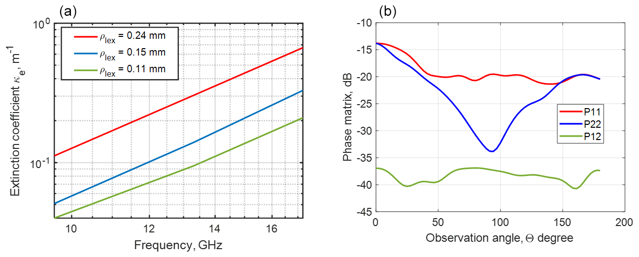
Figure 3 (a) Frequency dependence of the extinction coefficient from X- to Ku-band and (b) phase matrices at 13.3 GHz for different values of microstructure correlation length ρ_lex. Snow parameters are volume fraction f_v=0.20, aggregation parameter b=1.2, and correlation length 0.15 mm. P11 and P22 are co-polarized phase matrix elements, and P12 is a cross-polarized phase matrix element.

EM models thus have evolved in part due to knowledge advances from our improved ability to measure snow microstructure. Stereological approaches led to advances in treating snow as a random medium using correlation functions (Wiesmann et al., 1998). X-ray micro-computed tomography (µ-CT) has emerged to image the three-dimensional structure of snow (Kerbrat et al., 2008), as illustrated in Fig. 2c, which has fed advances such as the dual active–passive Snow Microwave Radiative Transfer (SMRT) model (Picard et al., 2018). SMRT was developed to understand how to represent microstructure faithfully at scales relevant for microwave scattering and has the potential to allow direct use of correlation functions from µ-CT. Application of µ-CT-derived microstructure parameters in SMRT removes the need for empirical grain-scale factors with frequency-dependent model performance governed by the quality of microstructure model fit (Sandells et al., 2021). EM models have been adapted to work with field-derived measurements as well. Field methods to measure microstructure are more fully discussed in Sect. 3.3.1. It is to be noted that the random medium model and the bicontinuous model both use the autocorrelation function. These advances reduce the uncertainties in interpreting remote sensing observations and support the design of remote sensing missions to observe seasonal changes in snow storage.

Figure 3 illustrates the volume scattering of snow with bicontinuous DMRT. Figure 3a shows the frequency dependence of the extinction coefficients κ_e for different values of microstructure correlation length and with aggregation parameter b=1.2. The results show the increase in extinction with increasing correlation length. The exponential of the frequency dependence is 3.3 from X- to Ku-band, which is less than the fourth-power law of Rayleigh scattering. This difference is due to the dense-media effect, and the power law exponent is found to depend on the aggregation parameter b. The phase matrices at 13.3 GHz for snow are shown in Fig. 3b. The phase matrix gives bistatic scattering as a function of the angle Θ between the incident direction $\widehat{s}$ and scattered direction ${\widehat{s}}^{\prime }$. In Fig. 3b, P11 and P22 are co-polarization phase matrix elements, and P12 is the cross-pol phase matrix. The phase matrix exhibits a dipole scattering pattern. The cross-polarization P12 is much larger than would be calculated by the sphere models because of the irregular shapes of the aggregates in the bicontinuous medium. The computed phase matrix and the extinction coefficients are substituted into the RTE, which is then solved to calculate backscattering. The results in Figs. 4–6 are an illustration of the bicontinuous model (Tan et al., 2015). The results as a function of SWE for a homogenous snow layer are shown in Fig. 4 for six channels with VV polarization at 10.2, 13.3, and 16.7 GHz in Fig. 4a and VH polarization for the same frequencies in Fig. 4b. In Chang et al. (2014), the results were compared with the Finnish NoSREx backscattering dataset, within which tower measurements were taken over snowpacks with SWE up to 120 mm. The bicontinuous-DMRT model results are in good agreement with backscatter observations over the six channels of multiple frequencies and polarizations, albeit with a frequency-dependent bias for the cross-pol results. Both the model predictions and measurements show high correlations with SWE with stronger correlations at 13.3 and 16.7 GHz than at 10.2 GHz. Several years of NoSREx data were analyzed, and the results of retrieval performance on the data were illustrated in the paper by Zhu et al. (2018).

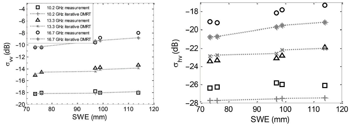
Figure 4 Comparison of the DMRT/bicontinuous media model using NoSREx 2010–2011 data backscatter against SWE for vertical co-pol (left) and cross-pol (right) at 10.2, 13.3, and 16.7 GHz. Figures are adapted from Tan et al. (2015).

1. Because of snow accumulation events and weather patterns, snow cover can have layering structures that correspond to variations in snow densities and grain sizes. Extensive work has been done in studying multilayered models of snow using the HUT model (Lemmetyinen et al., 2010), the DMRT-ML model (Picard et al., 2013), and the MEMLS model (Proksch et al., 2015a). Recent experimental work indicates that multilayered radiative transfer modeling may shed light on snow radar interaction (Thompson and Kelly, 2021a, b). For the case of DMRT, a multilayer DMRT model with different dense-media phase matrices and extinction coefficients for each layer is used (Liang et al., 2008; Chang et al., 2014; Tan et al., 2015). Both the quasi-crystalline approximation (QCA) model and the bicontinuous model have been used for a multilayer snow medium (Chang et al., 2014)

2. Structural anisotropy is a characteristic feature of natural snowpacks (e.g., Leinss et al., 2020). This causes changes in the phase matrix with the incidence angles and scattered angles. There are two models in the bicontinuous model: isotropic correlation functions and anisotropic correlation functions (Tan et al., 2016). Both have been developed and simulations performed. In the retrieval, only the isotropic correlation function versions have been used in the DMRT LUT.

3.1.2 Interaction of radar waves with the ground surface beneath snowpack

Because the dielectric contrast between dry snow and soil exceeds that between dry snow and air, the contribution of rough surface scattering arises primarily from the snow–soil rough interface and not from the air–snow interface (although it is noted that the air–snow interface may have a stronger scattering contribution when the snow is wet, but this is outside the domain of SWE retrieval using X- or Ku-band volume scattering). Rough surface scattering from the snow–soil interface contributes to radar observations as indicated by the term ${\mathit{\sigma }}_{bg}^{pq}\exp \left(-\mathrm{2}\mathit{\tau }\sec {\mathit{\theta }}_t\right)$ in Eq. (1). This term is affected by the rough soil surface scattering ${\mathit{\sigma }}_{bg}^{pq}$ and by attenuation through the snow exp (−2τsecθ_t). The rough soil surface scattering contribution is not related to SWE and therefore should be removed when retrieving SWE. A “subtraction” of surface scattering has been used to improve the accuracy of SWE retrieval (Zhu et al., 2018). The approach for removing ${\mathit{\sigma }}_{bg}^{pq}\exp \left(-\mathrm{2}\mathit{\tau }\sec {\mathit{\theta }}_t\right)$ involves a combination of data and electromagnetic models and is a significant part of the retrieval algorithm that is discussed later in this section. Here we discuss methods for calculating scattering from the snow–soil interface at L-, C-, X-, and Ku-bands.

Classical physical models for rough surface scattering include the small perturbation method (SPM) and the Kirchhoff approach (Ishimaru, 1978; Tsang and Kong, 2001). Advanced analytical methods include the advanced integral equation model (AIEM; Chen et al., 2003) and small-slope approximation and its extensions (Voronovich, 1994; Elfouhaily and Johnson, 2007). Fully numerical solutions based on the use of Monte Carlo simulations are also available to avoid approximation in the electromagnetic physics. In all these models, surface roughness can be described in part using the parameter kh, which is the product of the EM wavenumber k of the medium above the rough surface and the surface rms height h. Previous studies using analytical models and numerical simulations for snow or land sensing applications have emphasized cases having kh<3 due to a past focus on L-band sensors. For example, using a time series of SMAP VV- and HH-polarized backscatter measurements, both the surface soil moisture and surface rms height were retrieved at 3 km resolution for the 13 April–7 July 2015 period of SMAP radar operation (Kim et al., 2017). Results from this product show a global median surface rms height of 2 cm, with rms heights up to 5 cm in mountain regions. A surface rms height of 5 cm at 17 GHz would represent a kh value of 18 for the air–soil interface and 21.6 for the snow–soil interface (the larger value for the snow–soil interface is due to the larger electromagnetic wavenumber in snow). Past studies emphasizing kh<3 therefore limit applications to L- or C-bands. Recently, we have performed numerical surface scattering simulations having kh up to 15 (h=4.16 cm for 17.2 GHz) to widen the applicability of full-wave simulations up to Ku-band (Zhu, 2021; Zhu et al., 2021b​​​​​​​)

Surface scattering models typically describe the soil surface as a stationary Gaussian random process so that knowledge of its covariance function is sufficient to describe its properties. The covariance function is further parametrized in terms of its rms height and correlation length. Ground measurements have been made of these properties (Oh et al., 1992; Oh and Kay, 1998; Ulaby and Long, 2015), and measured correlation lengths are typically found to be limited to a maximum of 10 cm. We label these roughness measurements as “limited correlation length up to 10 cm”. However, in the global retrieval of soil moisture using 6 months of the NASA Soil Moisture Active Passive (SMAP) radar data at L-band, the roughness was modeled as having a constant correlation-length-to-rms-height ratio (Kim et al., 2012, 2014, 2017) that ranged from 5 to 20. These two methods for describing the correlation length differ significantly for rms heights beyond 2 cm; our studies have found that the constant-ratio approach gives more acceptable results. Surface scattering also depends on the soil permittivity, which in turn depends on soil moisture (which describes the volume of water present per unit volume of soil) and texture (which describes soil composition). Given these parameters, empirical models (Mironov et al., 2004; Peplinski et al., 1995) are available to calculate the soil permittivity. In addition to soil properties, land cover including litter and vegetation, as well as rock outcrops, impacts the spatial variability in surface permittivity and backscattering.

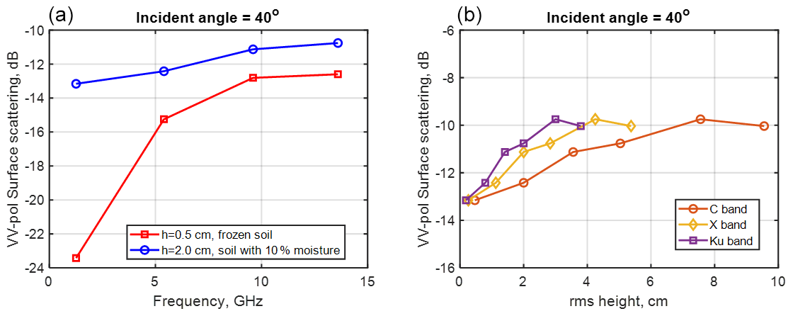
Figure 5 (a) Backscattering at VV polarization as a function of frequency: red curve is results with frozen soil (permittivity 4+1i) and rms height of 0.5 cm, and blue curve is results with soil of 10 % moisture and rms height of 2 cm. (b) Backscattering at VV polarization as a function of rms height with soil of 10 % moisture at C-, X-, and Ku-band.

Full-wave simulations based on numerical solutions of Maxwell's equations (NMM3D) were applied to L-band radar backscatter analysis for the SMAP mission (Huang et al., 2010; Huang and Tsang, 2012). The full-wave simulations were used to generate a look-up table (LUT; Liao et al., 2016). The LUT was initially used for the air–soil interface. Also, the LUT was based on the incident angle of the upper medium and the relative dielectric constant between the two media on the two sides of the rough surfaces. By adjusting the relative dielectric constants and the incidence angle using Snell's law, the NMM3D LUT can also be applicable for all combinations of relative dielectric constants including snow–soil, air–snow, or snow–permafrost interfaces, among others.

In Fig. 5a, we plot VV backscattering as a function of frequency for h=0.5 and 2 cm. In Fig. 5b, we further plot the VV backscattering as a function of rms height at C-, X-, and Ku-bands. Both figures show saturation effects, meaning that the rough surface scattering saturates at large rms heights (∼ 3–6 cm) and at higher frequencies. The new results of kh up to 15 are useful for studying rough surface radar backscattering at X- and Ku-bands for snow–soil interfaces.

To estimate rough surface scattering at X-band and Ku-band, there are two approaches labeled (a) and (b) in what follows. Approach (a) uses snow-free radar observations at X- and Ku-bands at a specific location to estimate the surface backscattering (Rott et al., 2010). Such an approach neglects any changes in soil properties and background land cover during the snow-on season. In approach (b), surface backscattering is estimated using a combination of measurement data and electromagnetic models. The measurement data include backscattering data at L-, C-, X-, and/or Ku-band under snow-free or snow-on conditions, and the NMM3D LUT is used to model surface backscattering. As a first step, co-polarized radar time series observations at L- and C-band, which have greatly reduced sensitivity to snow volume scattering, are used to estimate the soil permittivity and surface roughness. The use of a C-band-measured time series together with the past L-band time series data enhances the existing L-band algorithm in retrieving rms height and soil moisture, and the retrieval is performed in either the presence or absence of snow. When snow is present, Snell's law is used to adjust the incident angle at the snow–soil interface to account for the snow refraction effects. The surface rms heights and soil permittivities obtained are then used in the NMM3D LUT to predict the surface backscattering contribution $({\mathit{\sigma }}_{bg}^{pq}$) at X- and Ku-bands; note this captures any dynamically varying roughness or permittivity conditions in performing the surface scattering correction. We assume the availability of matchup L- and/or C-band SAR observations with revisit periods of approximately 10 d, as are or will be available from the Sentinel-1 and NISAR systems, as well as future proposed continuation missions, so that such datasets are likely to be available during the time frame of a future snow observing mission.

Consider for example L-band UAVSAR radar full-polarization observations under snow-on conditions (Liao et al., 2016). The UAVSAR dataset examined was collected from February to March 2017 in the SnowEx 2017 campaign using five flights over the Grand Mesa region in Colorado, United States. In situ soil moisture measurements were also collected throughout 2017 from an installed meteorological observation station. We apply the time series retrieval algorithm developed for the SMAP mission (Kim et al., 2012, 2017) based on the NMM3D LUT at the station location (i.e., at a point location). From the retrieved soil permittivity, the soil moisture is derived using Mironov's empirical model (Mironov et al., 2004). The comparison of retrieved and measured soil moisture is shown in Fig. 6a. The retrieval soil moisture is in good agreement with the measured in situ soil moisture for a period of 8 weeks from 6 February to 31 March 2017. In addition to retrieving the soil moisture time series, the rms height at this location was also retrieved and estimated as 1.9 cm. Note the Kim et al. (2017) algorithm retrieves a single rms height estimate for the time series because surface roughness is assumed to remain constant over the time series duration (so that wet and frozen soils are assumed to have the same rms height).

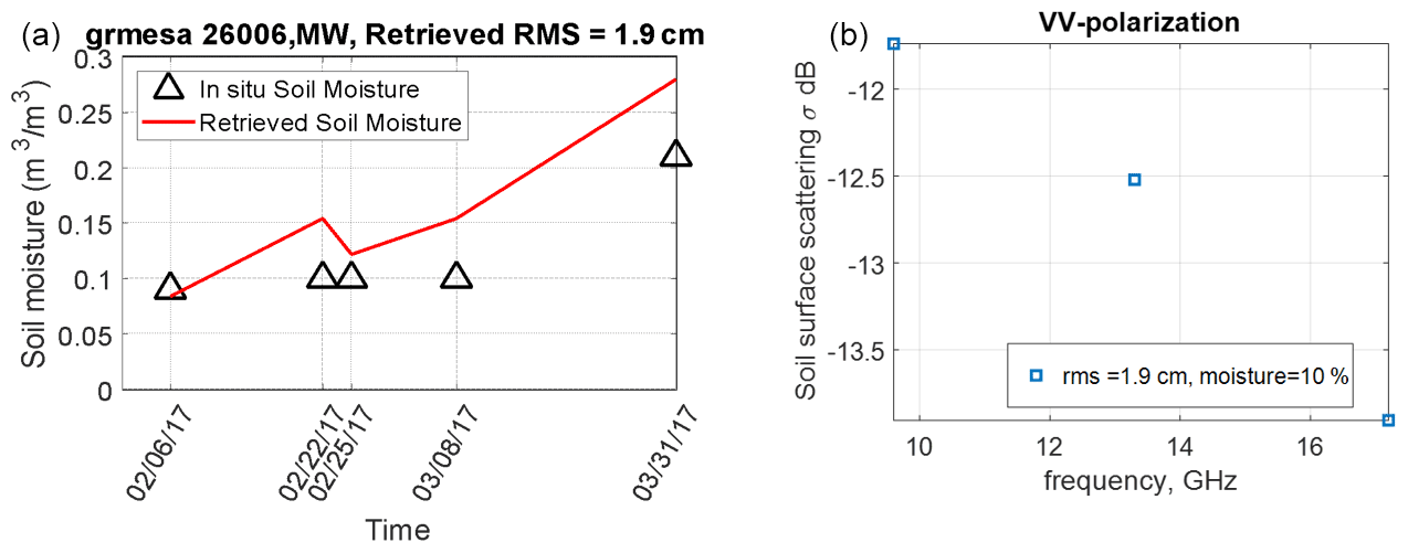
Figure 6 (a) Retrieval of soil moisture compared with in situ measurements. The retrieved rms height is 1.9 cm. The retrieval is based on based on L-band UAVSAR data from the SnowEx 2017 campaign. The measured soil moisture is from SnowEx 2017 campaign meteorological observations with a measured soil temperature of 0.6 ^∘C. The location of the station is 39.03388^∘ N, 108.21399^∘ W, with an elevation of 3033 m. (b) Simulated surface scattering with snow attenuation from X- to Ku-band at VV polarization. Snow parameters are with depth of 54 cm, density of 183 kg m⁻³, 〈ζ〉=1.2 mm, and b=1.2. Blue marks are based on the SnowEx 2017 campaign data shown in (a).

We next apply the retrieved rms height (1.9 cm) and the soil properties from Fig. 6a to calculate the surface scattering contributions with snow attenuation, ${\mathit{\sigma }}_{bg}^{pq}\exp (-\mathrm{2}\mathit{\tau }\sec {\mathit{\theta }}_t)$, at 9.6, 13.4, and 17.2 GHz as shown in Fig. 6b. The results show that the rough soil surface scattering contribution, including snow attenuation, is around −12 dB at X-band and decreases to −14 dB at 17.2 GHz; higher frequencies such as Ku-band typically experience higher volume scattering and greater attenuation of the surface scattering contributions. Continued studies are required to improve and validate this approach, including extending NMM3D surface modeling studies and the associated LUT into cases with rms heights of four wavelengths or more so that the LUTs can be applied at 17.2 GHz for rms heights up to 7 cm. Also, unlike snow volume scattering, rough-surface scattering has a stronger dependence on incidence angle and polarization. Thus, the effects of topographical slopes that cause changes in incidence angles, particularly in mountainous regions, should be included in the retrieval. Although it is noted that the sample size in Fig. 6a and b is small, the increasing availability of L- and C-band time series measurements and the extension of full-wave simulations from L-band to Ku-band up to kh=20 are expected to make the retrieval of surface rms heights and permittivities feasible so that robust surface scattering corrections can be achieved at X- and Ku-bands. Further extensions to consider the snow–permafrost interface are also under development.

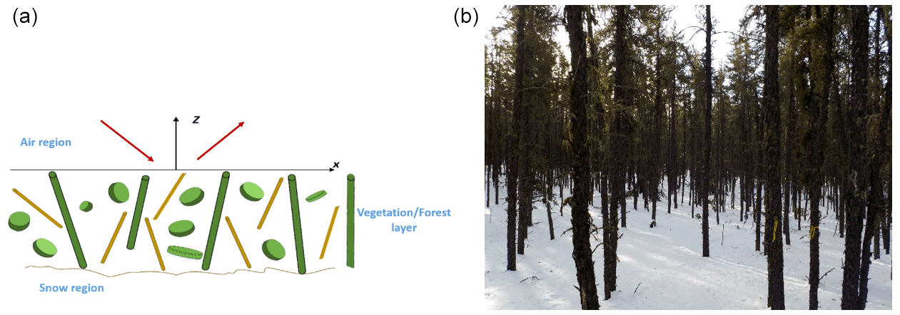
Figure 7 (a) RTE assumption: uniformly randomly positioned scatterers which are statistically homogeneous. (b) Illustration of trees for a forest with snow cover beneath. The picture was taken on 14 March 2017 in a Jack Pine stand situated in the Boreal Ecosystem Research and Monitoring Sites (BERMS), Saskatchewan, Canada.

3.1.3 Interaction of radar waves with forests and vegetation above snowpack

The interaction of radar waves with vegetation initially began with the water-cloud model (Attema and Ulaby, 1978) (Fig. 7a). It was then extended by using RTE to include scattering effects in addition to absorption. Computation codes of RTE exist such as the MIMICS model (Ulaby et al., 1990) and in the Torgata model (Ferrazzoli and Guerriero, 1995; Ferrazzoli et al., 1999). In addition, the discrete-scatterers model using distorted Born approximations (DBAs) has been used (Lang and Sighu, 1983; Karam et al., 1992). The RTE and DBA models use the same assumptions and give the same results aside from a factor of 2 in the double bounce of the volume–surface interaction term. Bindlish and Barros (2001) applied the water cloud model formulation to the parameterization of vegetation backscatter from C- and L-band radar measurements using three vegetation parameters (a measure of vegetation density, a measure of vegetation architecture, and a dimensionless vegetation correlation length) to characterize different types of vegetation in rangeland, winter wheat crops, and pasture. They found that the estimation of land-cover- and land-use-class-specific parameters resulted in significant improvements in retrieval of soil moisture, which suggests that a similar approach could be used for snow retrieval using multifrequency data along with detailed ancillary vegetation datasets to estimate the place-based parameters for the water-cloud model. Zoughi et al. (1986) conducted X-band radar measurements to identify the contributions from leaves, petioles, twigs, and branches of pine, oak, sycamore, and sugar maple trees to backscatter and attenuation. In addition to quantitative differences related to tree architecture and vegetation moisture content, they reported that the backscatter is mainly produced by the top layers of the canopy; petioles (tree microstructure) can significantly affect backscatter depending on their size relative to wavelength; and leaves play an equally important role in attenuation and backscatter, whereas twigs and branches dominated in terms of backscatter with weak attenuation when leaves were not present. They did not consider the effect of tree trunks.

In CoReH₂O Phase A the impact of forests on radar signals of snow-covered ground was studied (ESA, 2012). Model and data analyses were carried out by Kugler et al. (2014) and Montomoli et al. (2016). The forest model selected in CoREH2O is based on the radiative transfer equation (RTE). It accounts for scattering of trunks and branches of different size and needles as well as for differences in the structure of vertical layers. Effects of differences in cover fraction, tree height, and biomass were analyzed. The model gives a multifaceted description of forest properties and for estimating the impact of the forest parameters on the backscatter of snow-covered forests. The CoREH2O RTE-based studies indicate that, during the winter period, the presence of dormant herbaceous or short vegetation has small contributions to backscattering and does not affect the sensitivity to SWE. For the effects of coniferous forests (CFs), the simulation results show that in the case of low fractional cover of CFs (<25 %), contributions of snow volume scattering are the dominant contributions to the radar signal, with the radar signals correlating with SWE. When the forest density or the fractional cover increases, the sensitivity to SWE decreases. The sensitivities are much affected by CFs larger than 75 %. In addition to forest density and structure, snow interception in the canopy can vary widely in time and depending on snow type and canopy architecture, and it can modify the transmissivity and scattering characteristics.

Recently, since 2017, instead of using the RTE/DBA models, we have used full-wave simulations based on a hybrid method of combining wave multiple-scattering theory (W-MST) and commercial software in computational electromagnetics such as HFSS and FEKO. The “waves” MST is based on Maxwell's equations and different from that of multiple scattering in RTE, which only considers incoherent multiple scattering of leaves branches, for example. Full-wave simulation results have been computed for L-, S-, and C-bands.  The results of full-wave simulations show two distinct differences from that of the results of the RTE/DBA model: (i) the full-wave simulations show more penetration than predicted by the RTE model with differences that can be several times larger, and (ii) the full-wave simulations show weaker frequency dependence than the RTE model. We cannot at this moment extrapolate the conclusions to X-band and Ku-band for trees. However, preliminary results running full-wave simulations of needle leaves at X-band and Ku-band show significant differences from the RTE model. Thus, in the near future, there will be extensive full-wave simulations and new measurements to study the effects of trees and forests at X-band and Ku-band.

The reasons for the differences are that the basic DBA/RTE have two basic assumptions.

The first assumption is that scatterers such as trunks, leaves, primary branches, secondary branches, tertiary branches, etc. are individual, isolated scatterers that are uniformly positioned in the layer, such as that shown in Fig. 7a. The reason for this assumption is that the RTE model was first used for microwave remote sensing of cloud and rainfall. The assumption of uniform random positions is the same as homogenization, meaning that there is an effective attenuation rate κ_e. For a forest height of d, the Beer–Lambert law or the Foldy approximation states that the transmission through forest and vegetation is given by the expression $e^{-\mathit{\tau }\sec {\mathit{\theta }}_{\mathrm{i}}}$, where the optical thickness τ is equal to κ_ed.

However, in forests, such as coniferous forests (Fig. 7b), aspen forests, and deciduous forests, the scatterers are aggregated in trees. Unlike clouds, which do not have gaps, there are gaps between the trees. Thus, waves, such as those in the Ku-band at 17.2 GHz with wavelengths of 1.74 cm, can pass through gaps when gap sizes are larger than these wavelengths. The consequence of the assumption is that RTE underestimates the transmission. The second assumption is that the leaves and branches are assumed to be single scatterers, and they scatter independently. The extinction coefficients and phase matrices of Eq. (2) are calculated by adding the scattering cross-section of the branches and leaves. This assumption is valid for cloud and rainfall as the water droplets can be assumed to be single scatterers. However, the geometry (Fig. 7b) is that the branches and leaves are attached to the tree. For a coniferous forest, there are primary branches and secondary branches attached to a tree. The needle leaves are aggregated and are attached to branches. Thus, the entire tree itself should be treated as a single scatterer rather than an individual branch or an individual leaf. Therefore, the phase matrix of a tree should be used rather than incoherently adding the scattering cross-sections of branches, leaves, and the trunk for a tree. Using a tree as a single scatterer gives results that have weaker frequency dependence than that predicted by RTE/DBA.

Full-wave simulations to solve Maxwell's equations among trees or plants were deemed to be computationally formidable. Recently, a computationally efficient hybrid method (HB) has been developed to perform full-wave simulations (Huang et al., 2017, 2019; Gu et al., 2021, 2022). The hybrid method is a combination of commercial off-the-shelf software of computational electromagnetics, the Foldy–Lax wave multiple-scattering equations, and iterations based on the averaged multiple orders of scattering. The hybrid method consists of three steps. In the first step, a plant or a tree is treated as a single scatterer. Commercial off-the-shelf software is used to calculate the scattering T matrix in vector cylindrical waves of a single plant or a single tree. We have used the commercial software of HFSS and FEKO (Altair FEKO: https://www.altair.com/feko/, last access: 21 July 2022). In the second step, coherent-wave multiple-scattering theory (W-MST) among the plants and trees is formulated by using the Foldy–Lax multiple-scattering equations. The formulation uses T matrices and the vector addition theorem of vector cylindrical waves (Tsang and Kong, 2001​​​​​​​). In the third step, the Foldy Lax equations are iterated to obtain solutions in multiple orders of scattering, and averages are taken over realizations after several orders at a time to obtain the averaged solution. The third step makes use of the property that the averaged solution of orders of multiple scattering has faster convergence than obtaining the exact solution of a single realization through matrix iteration methods such as conjugate gradient or bi-conjugate gradient. NMM3D full-wave methods and simulation results can be found in Huang et al. (2017, 2019) and Gu et al. (2021, 2022). Below we illustrate two examples.

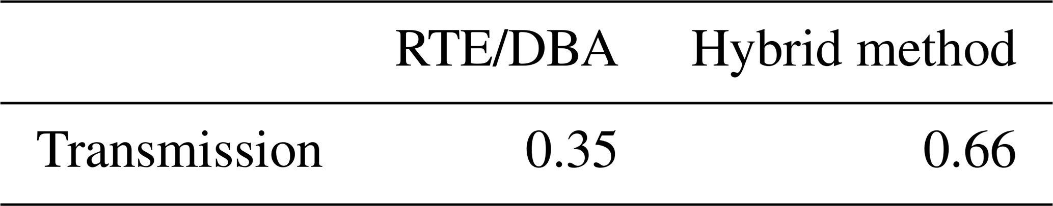
Simulations were performed for the transmission through a simulated forest (Huang et al., 2019) consisting of 196 cylinders representing tree trunks. Each cylinder is of 20 m height and 12 cm diameter, and the cylinder area is arranged as shown in Fig. 8. The results are tabulated in Table 1. The results show that the transmission is almost twice that of RTE.

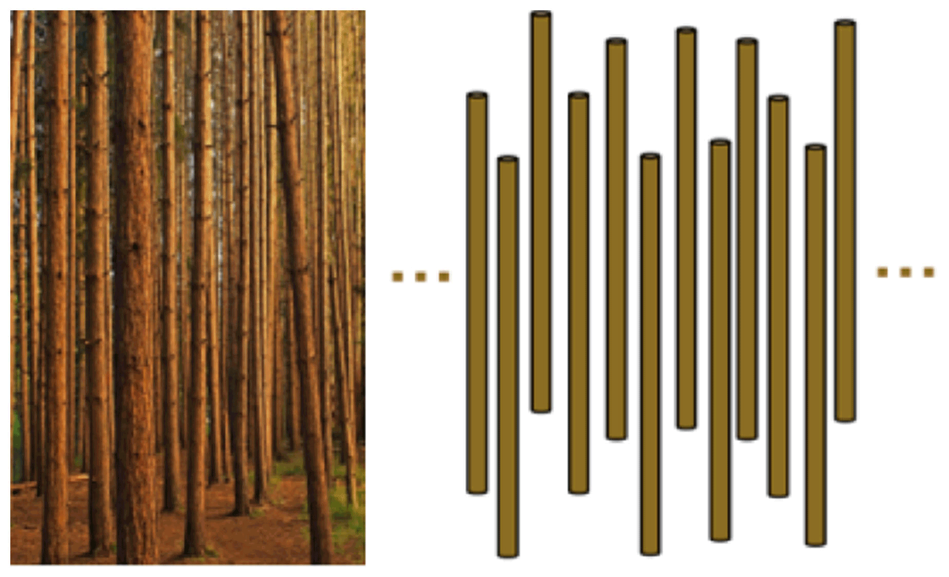
Figure 8 Tree trunks (left) are modeled as dielectric cylinders (right). The figure is adapted from Huang et al. (2019).

Table 1 Transmission coefficient from RTE based on distorted Born approximation (RTE/DBA​​​​​​​) and the hybrid method from Fig. 8. The table is adapted from Huang et al. (2019).

To consider frequency dependence, we next show an example of the transmission through a field consisting of 196 wheat plants (Fig. 9a) at L-, S-, and C-bands (Gu et al., 2021, 2022) as a function of volume water content (VWC). Results of Fig. 9b are compared with RTE. Firstly, the results show that the transmission of full-wave simulations is much larger than RTE. Secondly, the transmission at C-band is only slightly less than that at S-band, showing that the frequency dependence is weak between S-band and C-band. On the other hand, RTE shows a big drop in transmission from S- to C-band, indicating that RTE predicts a strong increase in attenuation with frequency from S-band to C-band. On the other hand, the full-wave simulation results have little difference between S-band and C-band, showing “saturation” with frequency. The example of wheat is shown to illustrate that RTE/DBA underestimates the transmission through vegetation and has a higher frequency dependence when compared to the hybrid method as shown in Gu et al. (2021, 2022). There are not many new published results using NMM3D for different types of vegetation to be shown in this review paper. However, there has been tremendous improvement recently in computational EM efficiency, and we expect new NMM3D results in the near future.

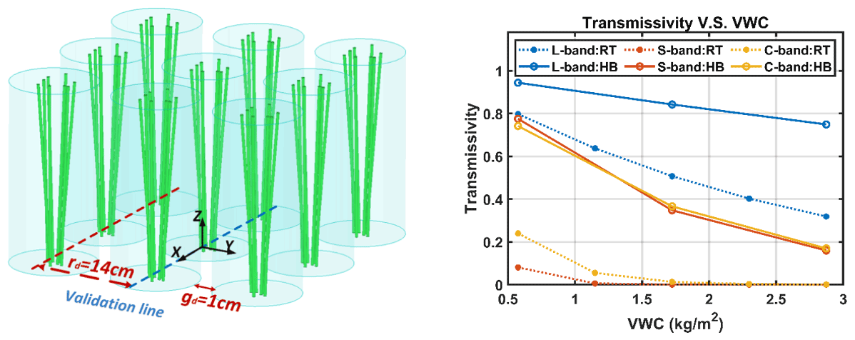
Figure 9 (a) Scattering from wheat plants is the radius of the circumscribing cylinder (6.5 cm), distance between the centers of two circumscribing cylinders is r_d=14 cm, and the closest distance between two circumscribing cylinders is g_d=1 cm. The figure is adapted from Gu et al. (2021). (b) Transmission of microwave through wheat of different orientation calculated using the hybrid method and the RTE varies with volume water content (VWC).

At Ku-band (17.2 GHz), the wavelength is 1.74 cm, which is much smaller than the gaps in trees. The wave can travel in straight lines as rays through the gaps. In such a scenario, the Ku-band waves will travel like the case of lidar, which has been shown to be able to penetrate forest canopies. In wireless communication, ray tracing has been performed as a path-loss model in forests (Ling et al., 1989; Kurt and Tavli, 2017​​​​​​​). However, ray tracing, in the opposite extreme of RTE, has no frequency dependence, although frequency dependence can be introduced in an ad hoc manner such as by only keeping the dominant scatterers at the operating frequency.

3.2 Experimental measurements of radar–landscape interactions

Collection of experimental data is a prerequisite for the development of Earth observation satellites. Ground-based and airborne sensors provide means to collect observations of the geophysical parameter of interest in a relatively controlled environment. These measurements provide the basis for the validation of forward-modeling approaches and development of retrieval algorithms prior to launch of the spaceborne mission. The measurements also help to understand the spatial resolution and temporal requirements for a spaceborne mission.

Ground-based sensors deployed on tower structures allow near-continuous observations over extended periods, which are critical for understanding both slow and seasonal processes as well as rapid phenomena induced by diurnal changes at the sensor footprint. Such temporal features are of particular importance for seasonal snow cover. Airborne observations, or the deployment of ground-based sensors on other mobile platforms, provide the ability to expand localized observations to a larger scale, allowing the effect of heterogeneous land cover and vegetation on Earth observation signatures to be observed. Seasonal snow presents a particularly challenging target for observations due to the high variability in snow over both temporal and spatial scales. Hence, several localized and ground-based campaigns as well as airborne sensor deployments have been conducted in recent years in an attempt to understand radar signatures from seasonal snow cover. These campaigns have covered diverse snow and climatological conditions.

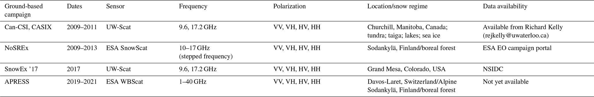
Table 2 Summary of ground-based active microwave sensors for snow studies.

3.2.1 In situ radar experiments and signatures

The ground-based campaigns are summarized in Table 2. Ground-based campaigns of Can-CSI and CASIX were conducted between 2009 and 2010, and multiple field campaigns were completed near Churchill, Manitoba, Canada, as part of the Phase A science activities of CoReH₂O. These campaigns aimed to evaluate the potential for dual-frequency X- and Ku-band snow property retrievals in subarctic environments. Central to Churchill campaigns was deployment of the University of Waterloo Scatterometer (UW-Scat), a novel ground-based radar system analogous to the proposed configuration of CoReH₂O (King et al., 2012). In Europe, ESA initiated the deployment of SnowScat (Werner et al., 2010), a stepped-frequency, fully polarimetric ground-based radar in a series of campaigns in the boreal forest zone in northern Finland (Lemmetyinen et al., 2016). The campaign was called NoSREx and operated SnowScat over four winter seasons, complemented by passive microwave radiometry and regular snow microstructural observations. These campaigns have been instrumental in enhancing our understanding of snow–microwave interactions and providing data to develop and evaluate forward models simulating backscattering from snow cover (King et al., 2015; Tan et al., 2015; Proksch et al., 2015a), as well as developing retrieval approaches (Cui et al., 2016; Lemmetyinen et al., 2018).

In Sect. 3.1.1, we make use of the NoSREx campaign's six channels of backscattering data of VV at 10.2, 13.3, and 18.7 GHz and HV at 10.2, 13.3, and 18.7 GHz in comparison with the simulation results of bicontinuous-DMRT models. The comparisons have validated both the ground campaign measurements and the physical models (Tan et al., 2015).

Recent ground campaigns include APRESS, in which the ESA WBScat instrument, a full-polarization radar operating at 1–40 GHz, was deployed for a full winter season in 2019–2020 measuring an Alpine snowpack in Davos, Switzerland. For the winter of 2020–2021, the instrument was set up in Sodankylä, Finland, to collect data over a sparsely forested site. These sensors and deployments have generated and will continue to generate critical datasets for characterizing the radar backscattering of snow, the effects of rough surface scattering, and forests. They will help to advance retrieval development when coupled with advancements in field methodology and forward-modeling capabilities.

3.2.2 Airborne experiments and signatures

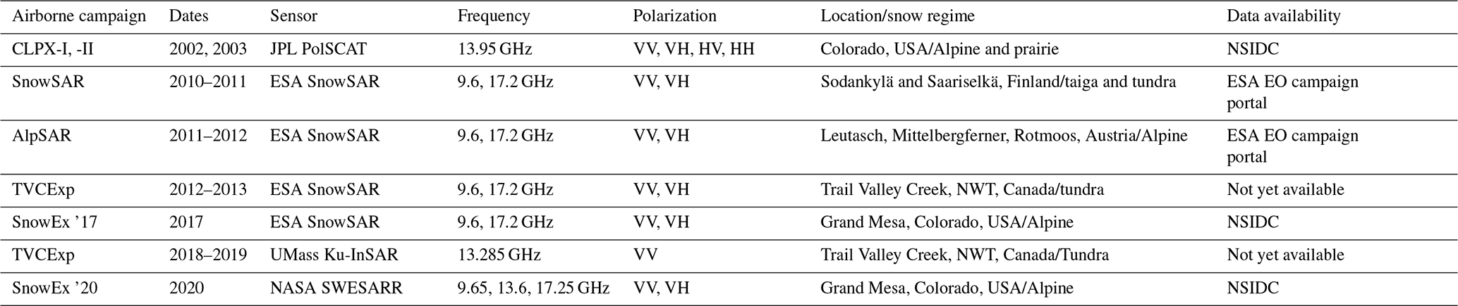
Airborne campaigns (listed in Table 3) provided the first experimental demonstration of the sensitivity of Polarimetric Ku-Band Scatterometer (PolSCAT) backscattering to SWE (Yueh et al., 2009). CoReH₂O provided further impetus for the development of new airborne sensors. The ESA SnowSAR, a dual-polarization, airborne, side-looking SAR operating at X- and Ku-bands (Coccia et al., 2011; Meta et al., 2012), was deployed at several sites in northern Finland, the Austrian Alps, northern Canada, and Alaska between 2011 and 2013.​​​​​​​ The purpose of the flight campaigns was to collect data over a range of climatological snow classes and land cover regimes. All flight campaigns were supported by extensive measurement of snow properties, including vertical profiles of snow stratigraphy and microstructure. The campaigns have enabled the further assessment of, for example, vegetation effects on backscatter (Cohen et al., 2015; Montomoli et al., 2016) and the effect of spatially variable microstructure (King et al., 2018) as well as the further elaboration of modeling and retrieval capabilities (Zhu et al., 2018). Figure 10 demonstrates the effect of changing snow conditions on the observed Ku-band co-polarized backscatter during two of the SnowSAR flights in Finland. The differences between open area and forested area have been addressed and illustrated in Montomoli et al. (2016) using the models of classical radiative transfer. Results of full-wave simulations are currently being studied.

Figure 10 Demonstration of observed Ku-band VV-pol backscattering from two consecutive SnowSAR flight campaigns in Sodankylä, Finland. The difference in backscatter is depicted on the right, with red implying an increase. Increases in measured backscattering are correlated with the increase in SWE. The measured SWE between the flights increased on average by 41 mm in non-vegetated areas, which show the highest increase (figure adapted from Lemmetyinen et al., 2014).

Recent airborne campaigns including SnowEx 2017, SnowEx 2020, and TVCExp 2019 have deployed a new generation of airborne systems to address known uncertainties including penetration in dense vegetation, background interactions, and interferometric SAR (InSAR) applications (Table 3). As part of ongoing research at Trail Valley Creek, a new Ku-band InSAR (13.285 GHz) developed by the University of Massachusetts was deployed during the winter of 2018–2019. This system was developed to allow rapid deployment aboard common commercial platforms, leading to three successful acquisition periods throughout the winter. Coupled with objective measurements of snow microstructure and a distributed network of soil permittivity sensors, these data are now being used to develop InSAR and backscatter retrieval methods for future missions. The Snow Water Equivalent SAR and Radiometer (SWESARR) is a tri-band synthetic aperture radar (SAR) and a tri-band radiometer. Both the active and passive bands utilize a highly novel current sheet array (CSA) antenna feed. SWESARR has three active (9.65, 13.6, 17.25 GHz) and three passive (10.65, 18.7, 36.5 GHz) bands. Radar data are collected in dual polarization (VV, VH), while the radiometer makes single-polarization (H) observations. During SnowEx 2020, NASA Goddard's SWESARR demonstrated for the first time that X-band, low-Ku-band, and high-Ku-band SAR acquisition can be made through a single antenna feed. Data collected during this campaign coincided with detailed measurements of vegetation structural properties and under-canopy snow properties that will be critical to address the effects of vegetation and forests in SWE retrieval.

Airborne campaigns are planned for 2022–2023 for both Canada and US SnowEx. These future campaigns will address the following questions. (a) What is the maximum forest density for retrievable SWE at Ku-band? Recent full-wave simulations using Maxwell's equations suggest that penetration through forests is higher than predicted by past models of radiative transfer. (b) What is the saturation maximum depth for retrievable SWE at X- and Ku-bands? Using cross-polarizations, can we have higher depth of penetration such as 1 to 3 m? (c) What is the impact of stratigraphy and how snow physics models can help to retrieve SWE in the presence of stratigraphy? (d) How would permafrost and the changing freeze depth in some areas affect the surface scattering contributions and the ability to subtract surface scattering estimated under snow-free conditions. With six measurements in SWESARR, which are co-polarization and cross-polarization at three frequencies, what are the optimum combinations of polarization and frequencies for SWE retrieval?

Table 3 Summary of airborne deployments of active microwave sensors for snow studies.

3.3 Linking field measurements of snow with theoretical models of snow–radar interactions

Quantification of physical snow processes through objective measurements has revolutionized our understanding of microwave interactions with complex snowpacks at multiple scales (millimeter to kilometer). Objective methods of determining snow grain size in the field have only been available over the last decade. Prior to this, grain size was typically quantified visually with a hand lens or microscope (Fierz et al., 2009) and could be subject to errors of up to 1 mm in grain size estimation (Leppänen et al., 2015). Laboratory processing methods include gas absorption (Legagneaux et al., 2002) and thin-section imaging techniques (Bader et al., 1939). As described in Sect. 3.1.1, µ-CT measurements of snow samples obtained in the field have revolutionized our ability to model EM interaction from snow. Today, field-based instruments can quantify the snow specific surface area (SSA) rapidly in the field through either near-infrared reflectance (e.g., Gallet et al., 2009) or penetrometry (Proksch et al., 2015b). SSA is often related to an effective sphere diameter, that is the diameter of a sphere with the measured SSA (Mätzler, 2002). In practice, these metrics must often be scaled to match output from radiative transfer models (Montpetit et al., 2012). In addition to advances in sensors, experiment design has advanced significantly in support of radar remote sensing measurements: Appendix A provides an example experiment design that has been used in recent field campaigns. In practice, the time requirements of faster traditional measurements with longer history must be weighed against the newer measurements, which are sometimes more time-consuming with fewer trained operators. Here, we describe how this new knowledge of microscale variability over seasonal timescales can be leveraged to inform algorithms applied at landscape scales.

3.3.1 Spatial variability in field measurements

At the landscape scale, understanding snow spatial variability is of critical importance with respect to the development of methodologies that can observe and model discrete and bulk properties of snowpack with low uncertainty. Mountains, hills, and valleys exert aerodynamic roughness controls on snowfall trajectory, enhancing snow accumulation and redistribution processes often dominated by blowing snow and sublimation. Exposed topography (e.g., Alpine areas or open upland plateaus) is typically scoured of snow, while enhanced accumulation is found in gullies or on the lee-side of plateaus (Pomeroy et al., 1993; Liston and Sturm, 1998). Once accumulated, the persistence of snow on the landscape is influenced by terrain slope and aspect, which control a snowpack's energy budget; the incoming heat energy to north-facing slopes is radically different to that for south-facing slopes that can lead to pronounced variations in SWE at the landscape scale (López-Moreno et al., 2014). Local slope angles also cause changes in the incidence angle of radar backscattering, which may impact assumptions underpinning microwave retrieval algorithms because rough surface scattering has a strong angular dependence.

The distribution of tree canopy, woody biomass, and the fragmentation characteristics of the vegetation stands play a significant role in how snow accumulates in a forested landscape. Metrics describing plant functional types (e.g., deciduous/coniferous or broadleaf/needleleaf, canopy densities and heights, etc.) are used to quantify spatial difference in simulations of sub-canopy snow and microwave radiative transfer. Correcting for forest microwave attenuation has shown that forest transmissivity plays an important role in the observability of the sub-canopy snow. However, transmissivity changes through the season as the woody biomass undergoes progressive cooling at temperatures below 0 ^∘C (Li et al., 2020). Moreover, observed transmissivity of a tree stand is also impacted by the forest gap fraction or forest fragmentation. Landscape metrics can be used to characterize these ecological factors using high-spatial-resolution active and passive optical observations (Vander Jagt et al., 2013). The impact of low-stand shrub vegetation is also important for snow accumulation in sub-Alpine, tundra, and sub-tundra regions and in the understory of forested environments. Shrub-dominated landscapes retain snow more effectively than graminoid plant cover but less than forest-covered regions (Marsh et al., 2010).

The soil type and state affect microwave observations of snow at the landscape scale because, at microwave wavelengths, the soil relative permittivity can play an important role in how reflected or backscattered energy is attenuated at the snow–ground interface. Generally, relative permittivity of soil is controlled by the texture, moisture content, and thermal heat content of the soil. Seasonal change in soil water state (liquid or frozen) is also important since relative permittivity changes significantly as the surface soil moisture changes state. This is all complicated by the variability in soil type at the landscape scale, and especially the mix of organic and inorganic content; peat soil landscapes are very complex in their microwave response, whilst inorganic soils are somewhat simpler to characterize. In agricultural landscapes, especially post-harvest, the surface soil layer tends to be more spatially uniform and freeze earlier, making the variations in relative permittivity of the soil relatively constant.

In SWE retrieval, the snow–soil rough surface scattering and the forest effects on transmission and backscattering give bias in radar measurements. It is important to evaluate the magnitudes of these effects and how such bias in radar measurements varies with time.

3.3.2 Seasonal variability

Temporal changes in snowpack properties have important implications for radar backscatter, in particular (1) snow mass change, (2) metamorphism of snow microstructure, and (3) liquid water content and refreeze (ice lenses). High-temporal-resolution (hourly) measurement of snow mass accumulation and ablation using snow pillows, e.g., SNOTEL (Yan et al., 2018), or passive gamma radiation SWE sensors (Smith et al., 2017) provides excellent evaluation data to test SWE retrieval algorithms. However, such point measurements of SWE are spatially limited, and seasonal variability in SWE is more commonly estimated through depth measurements, at a point using an acoustic sounder or spatially distributed from lidar, and periodically measured or modeled snow density. Uncertainties in modeled snow densities commonly dominate uncertainties in measured depth (Raleigh and Small, 2017).

Seasonal change in snow microstructural properties can strongly influence scattering of radar backscatter, especially in snowpacks of which depth hoar is a significant component. Constraining the proportions of snowpacks that have different scattering properties (e.g., surface hoar, wind slab, consolidated layers, indurated hoar, or depth hoar) is required to prevent the retrieval of SWE from backscatter becoming an ill-posed problem. Frequent (weekly) objective profiles in snow pits (Sect. 5.3) are optimal; however, in lieu of in situ pit measurements, thermistors situated at different heights above the ground that become sequentially buried in accumulating snow allow calculation of temperature gradients within the snowpack. Consistent temperature gradients can be used as a proxy for likely snow crystal type (Domine et al., 2008): rounded (<10 ^∘C m⁻¹), facets (10–20 ^∘C m⁻¹), depth hoar (>20 ^∘C m⁻¹). Where internal snowpack temperatures are not available, 2 m air temperatures and near-surface soil temperatures can provide bulk estimates of snow temperature gradients.

Profiles of liquid water content (LWC) are measured in situ through insertion of dialectic devices (Denoth, 1994; Sihvola and Tiuri, 1986) into a snow pit wall. LWC can also be retrieved through non-invasive techniques using only GPS signal attenuation (Koch et al., 2019) or electrical self-potential (Thompson et al., 2016). Where mid-winter melt events are observed, either directly from LWC measurements or via inference from meteorological inputs, the chances increase in ice lens formation within the snowpack, which is an important consideration for SAR backscatter retrievals. Snow wetness affects the radar backscattering (Stiles and Ulaby, 1980). The dielectric constants of wet snow have been modeled as a function of snow wetness (Ulaby and Long, 2015).

4 Characterization of snowpack properties using radar measurements

4.1 Describing the retrieval problem

In early studies, empirical models were proposed for SWE retrieval (Ulaby and Stiles, 1980; Drinkwater et al., 2001). These are unsuited for all snow types, e.g., ephemeral, prairie, maritime, and mountain snow. (Sturm et al., 1995). Later investigators applied multiple channel measurements to determine snow parameters (Shi and Dozier, 2000; Rott et al., 2010). Recent algorithms (Cui et al., 2016; Xiong and Shi, 2017; Lemmetyinen et al., 2018; Zhu et al., 2018; King et al., 2019) are based on physical models in which RTMs are used. Physical-model-based retrieval algorithms consist of three parts: (1) a physical model of snow volume scattering, (2) estimation of a priori parameters, and (3) a cost function inversion of the physical model to obtain SWE. An important limitation historically has been that there are fairly few in situ and airborne datasets on which to evaluate retrieval algorithms. This limitation is rapidly being overcome by recent observations, as described in Sect. 3.2. In this section, we describe the estimation of a priori parameters and SWE retrieval procedures.

Volume scattering of snowpack is a function of parameters including SWE, density, snow microstructure, and stratigraphy. Paramount for the success of the retrieval is the ability to predefine or constrain some of these unknown parameters, in particular the parameters that are used to characterize the snow microstructure. Based on the RTM, volume scattering is a function of snow depth, density, snow microstructure, and layering structure (Rott et al., 2010; Zhu et al., 2018; King et al., 2018). A challenge is the non-uniqueness in inversion as different combinations of SWE and parameters of snow microstructure can give similar backscattering (Tsang et al., 2004; King et al., 2018). A priori estimates of parameters of snow microstructure can be used to improve the accuracy of retrieval by constraining the cost function with estimated statistical uncertainties.

Assuming normal distributions for the errors in forward simulations and observations of backscatter, the cost function of a maximum likelihood estimate for SWE and snow microstructure can be formulated as follows:

$$\begin{array}{}\text{(3)}& \begin{array}{rl}F& =\left\{{\sum }_{i=\mathrm{1}}^N{\displaystyle \frac{w_{\mathrm{i}}}{\mathrm{2}{s}_i^{\mathrm{2}}}}{\left({\mathit{\sigma }}_i^{\mathrm{obs}}-{\mathit{\sigma }}_i^{\mathrm{model}}\left(\mathrm{SWE},x\right)\right)}^{\mathrm{2}}\right.\\ & \left.+{\displaystyle \frac{w_{\mathrm{X}}}{\mathrm{2}{s}_{\mathrm{X}}^{\mathrm{2}}}}{\left(x-\stackrel{\mathrm{‾}}{x}\right)}^{\mathrm{2}}\right\},\end{array}\end{array}$$

where ${\mathit{\sigma }}_i^{\mathrm{obs}}$ is radar observations from the ith channel, and N is the total number of channels for measurements. In CoReH₂O, N=4 for VV and VH polarizations of X- and Ku-band. The backscattering predictions of snowpack are given by ${\mathit{\sigma }}_i^{\mathrm{model}}$. In the above, $s_i^{\mathrm{2}}$ is the error standard deviations of the radar measurements. The parameter x is related to snow microstructure, such as single-scattering albedo, correlation length, and grain size; $s_{\mathrm{X}}^{\mathrm{2}}$ is the variance of a priori constraint. In Cui et al. (2016) and Zhu et al. (2018), s_i is assumed to be 0.5, which is based on the error standard deviations of radar measurements; w_i and w_X are the weighting factors in the retrieval. Dual-frequency retrievals are using either X- (9.6 GHz) and Ku-band of 17.2 GHz as in CoReH₂O or dual Ku-band of 13.6 and 17.2 GHz as currently being proposed (see Sect. 6). However, cross-polarizations have not been fully utilized, and algorithms have been using the two co-polarizations of the dual-frequency measurements. The two-frequency measurements exploit the frequency dependence of volume scattering in snow. The two parameters that strongly influence the backscattering measurements are SWE and snow grain size. Then the problem becomes retrieval of two parameters from two measurements.

The proposed algorithm in Eq. (3) has built off the CoReH₂O (Rott et al., 2010) approach. Such physically based retrieval approaches are quite general with (i) matching the data to the physical models and (ii) a priori constraints on parameters. The actual implementation can have wide varieties of options, and the importance is the validation against datasets of tower and airborne measurements. Since the 2012 CoREH2O ESA report, there have been significant airborne and ground campaigns, as shown in Tables 2 and 3, providing much more data than were available prior to CoReH₂O. In Sect. 4.3, we describe three algorithms that have been used successfully (Lemmetyinen et al., 2018; King et al., 2019; Zhu et al., 2018, 2021a​​​​​​​). In particular, we describe in more detail the algorithm in Zhu et al. (2018, 2021a​​​​​​​) and describe the validations with a series of tower and airborne measurements. In the CoREH2O cost function, there are several parameters that require a priori estimates. The algorithm in Zhu et al. (2018, 2021a) is more closely related to the NASA SMAP radar algorithm; by using regression to electromagnetic model simulations over a wide range of parameters, the number of parameters is significantly reduced. The strategy of this approach is to reduce the burden of a priori estimates of parameters for every scene. Nevertheless, it is important to stress that algorithms are still maturing.

4.2 Constraining the retrieval problem with prior information

Some of the challenges in retrieving snow properties from radar measurements can be addressed by using so-called “prior information”. Prior information introduced in a retrieval problem can be thought of in a Bayesian sense, as discussed by Pulliainen (2006), or as “regularization”. The cost function (Eq. 3) applies prior information as described in Sect. 4.1, where x represented a snow-microstructure-related metric for which prior information is applied based on the final term on the right of Eq. (3). More generally, priors could be applied to multiple terms in the retrieval problem including SWE, as done in the proposed CoReH₂O algorithm (ESA et al., 2012), or in a multilayer sense, as illustrated for passive microwave remote sensing by Pan et al. (2017).

The degree to which prior information is applied to a problem can be thought of as a spectrum: the most minimal use of prior information is to remove the prior from the objective function but to specify a range of possible values for each prior, as done by Thompson and Kelly (2021a). Specification of a prior on either grain size or single-scattering albedo can be considered moderate use of a priori information. The CoReH₂O mission proposal specified an algorithm with prior on effective grain radius and SWE (ESA et al., 2012), building on the approach of the GlobSnow data product (Luojus et al., 2021). Cui et al. (2016) similarly specified priors for both optical thickness (an analog for SWE) and single-scattering albedo (an analog for microstructure). Zhu et al. (2018) built on the approach of Cui et al. (2016) by requiring only a single prior on single-scattering albedo. The algorithm of Zhu et al. (2018) requires only a “classification” of high or low single-scattering albedo. Maximal use of a priori information would be to use a dynamic simulation of snow microstructure processes to inform the retrieval. The model could be run “offline” and provide information on microstructure, or radar observations could be assimilated directly as done by Bateni et al. (2013, 2015).

Several studies have attempted to characterize the required precision of the priors on microstructure. ESA et al. (2012) found that an effective grain radius would need to be known with 15 % of the true value. Rutter et al. (2019) similarly showed that microstructure would need to be known to within 10 %–15 % in order to accurately retrieve SWE for field data in a tundra snow environment. These requirements are daunting. However, other approaches have indicated that microstructure information may not be required to be so precise. Thompson and Kelly (2021a) showed a successful inversion of SWE from in situ radar measurements in a prairie snow environment using a cost function specified with only minimal prior information (as defined in the previous paragraph). The algorithm of Zhu et al. (2018) requires only the specification of whether the single-scattering albedo is high or low (i.e., because the specification of a priori information is changed from a continuous to a categorical problem, the burden of a high-precision prior is much alleviated). Bateni et al. (2013, 2015) demonstrated that maximal use of prior information in the context of an assimilation scheme could provide prior information from weather data and snow physics to successfully estimate SWE. Thus, even though the radiative transfer equations are highly sensitive to microstructure, and sensitivity analysis would indicate that priors must be specified to high precision, successful SWE inversions have been demonstrated without high-precision priors. In the following subsections we review two ways of specifying prior information.

4.2.1 Leveraging snowpack information and snow classes

The simplest approach to specifying microstructure prior information for global SWE retrievals is to recognize the differences in snow types globally. The classifications of Sturm et al. (1995) and Sturm and Liston (2021) specify differences in snow texture based upon temperature, precipitation, and wind speed. Wind speed is mediated in many environments primarily by forest canopy height, and thus these three indicators can be specified by available land cover and meteorological information, globally. Clearly defined physical processes such as vapor flux driven by temperature gradient link these three meteorological quantities to observable snow properties, such as the number of layers, vapor transport through the snowpack, and microstructure properties such as grain size. Sturm and Liston (2021) specify six snow classes: tundra, boreal forest, prairie, montane forest, maritime, and ephemeral globally at approximately 300 m spatial resolution. The relevance to microstructure properties is clear: tundra snow (e.g.) has far larger snow crystal size in its depth hoar layers than taiga snow. In order for retrieval algorithms to leverage the predicted snow class to define a priori estimates to guide SWE retrievals, objective microstructure information would need to be specified for each snow class. The updated snow class of Sturm and Liston (2021) and the maturity of the methods to objectively measure microstructure described in Sect. 3.3 have now made this a possibility that will guide SWE retrieval efforts from radar measurements in the future.

4.2.2 Snow microstructural models

Background

Across the electromagnetic spectrum, the interaction of radiation with snow cover is mediated by snow microstructure (West et al., 1993; Wiscombe and Warren, 1980; Nolin and Dozier, 2000). However, due to differing penetration depths, visible and near-infrared measurements are sensitive to grain size at the surface, whereas microwave measurements are sensitive to grain size at depth (Hall et al., 1986). The sensitivity of radar measurements to microstructure properties has been demonstrated by both models (Xu et al., 2012; Proksch et al., 2015a) and experiments (King et al., 2015; Rutter et al., 2019). Algorithms to retrieve SWE from radar backscatter typically solve for both SWE and some measure of snow microstructure (e.g., single-scattering albedo, correlation length), and regularization terms or prior information on microstructure is often included in the retrieval cost function (as described in the previous section; see Rott et al., 2010). In addition to important advances in measuring snow microstructure in the field, as described in previous sections, new work to simulate the evolution of snow grain size has indicated great potential for improving radar retrieval algorithms of SWE. In the cost function of the retrieval algorithm, the a priori estimate term is $\frac{w_{\mathrm{X}}}{\mathrm{2}{s}_{\mathrm{X}}^{\mathrm{2}}}{\left(x-\stackrel{\mathrm{‾}}{x}\right)}^{\mathrm{2}}$, with grain size being the most important a priori parameter.

To prevent confusion, it is important to begin with clear definitions for snow microstructure. Snow is a continuous, granular, bonded medium, composed of irregularly shaped ice crystals, water vapor, liquid water, and void areas. The term “microstructure” commonly refers to snow grain size, shape, bonding, and distribution. Snow microstructure evolves both vertically within a snowpack and temporally throughout the snow season (as well as exhibiting significant horizontal spatial variability). The dendritic forms of new snowflakes sublimate, leading to a wide range of rounded or faceted shapes, depending on snowpack conditions. For many years, snow microstructure was referenced by the term “grain size”. However, because “grain size” is an imprecise term, and because several metrics of snow microstructure play a role in radar backscatter, we simply refer to “snow microstructure” here to encompass all measures of the snow medium; see Mätzler (2002) for a formal description of the various microstructural quantities. The most important and objective measure of snow microstructure is the snow specific surface area (SSA), which is often defined as the surface area of the ice–air interface to the mass of a control volume of snow. SSA provides an objective measure that explains much of the microwave scattering processes. However, microwave interaction with microstructure cannot be entirely summarized by SSA; instead, radiative transfer is controlled by the spatial autocorrelation function (SAF) of the ice–air interface (Löwe and Picard, 2015). In the random medium model, the microstructure is described by a correlation function (Mätzler, 2002). In the bicontinuous-medium model and the spherical-scatterer models with stickiness, spatial correlation functions (SAF) have also been derived and have been related to the grain size and the aggregation parameter or the stickiness parameter (Chang et al., 2016). Thus, all microstructure characterizations in electromagnetic models can be related through the SAF. The SSA is a measure of the SAF at only the shortest spatial lags (e.g., ∼ 10 µm); radar waves also respond to SAF at longer lags (hundreds of microseconds​​​​​​​). The SAF can be estimated using laboratory methods, such as µ-CT. Grain shape can play an important role in scattering, especially for the cross-polarization radar terms (Yueh et al., 2009). In summary, SSA has emerged as a practical and important microstructural property that both explains much variability in microwave scattering and can be measured in the field.

Microstructure evolution schemes: how they work

SSA evolves based on well-understood physical properties, providing a source of information to better inform SWE retrieval from Ku-band radar. Accurately modeling snow microstructure is not trivial, but decades of pioneering work by Colbeck (1982), Sturm (1989), Brun (1989), Brun et al. (1992), and Jordan (1991), among others, led to the development of snow metamorphism laws rooted in mass and energy conservation. The gravitational settling and metamorphism laws govern the temporal evolution of snow microstructure and its mechanical (e.g., snow stratification and shear stresses) and thermal (e.g., albedo and emissivity) properties. The metamorphism laws describe three types of grain growth mechanisms including kinetic growth, equilibrium growth, and melt metamorphism (Lehning et al., 2002; Huang et al., 2012); kinetic and equilibrium growth are sometimes called constructive and destructive metamorphism, respectively.

Destructive metamorphism describes movement of water vapor from small grains with high curvature to larger grains with lower curvature. As a result, small grains and dendritic branches of large snow crystals evaporate and form larger and more spherical crystals. Constructive metamorphism is primarily driven by temperature gradients within the snowpack, resulting in direct vapor transport from warmer to colder surfaces. Sturm and Benson (1997) documented these processes in the Arctic. The snowpack temperature gradient, in turn, is simply the difference in temperature between the ground and the air, divided by the snowpack depth; typically snow covers insulate the ground, leading to soil being warmer than the ground. When snow is wet, the growth rate accelerates, compared with dry-snow conditions. These fundamental physical processes have been explored for decades, and solutions to the governing equations exist in a range of physical models.

Microstructure simulation accuracy

Snow microstructure model accuracy has improved significantly in recent decades, driven by improvements of field measurements and model techniques. Morin et al. (2013) used objective field-based measurements of snow specific surface area using the DUFISS instrument to evaluate the many-layer CROCUS snow model. Figure 11 clearly shows that the model captured the seasonal evolution of SSA. The r² fit values between observations and simulations ranged from 0.6 to 0.74.

Figure 11 Observed and interpolated SSA observations (a) and SSA simulations (b). From Morin et al. (2013). The small white marks are the observations.

Use of microstructure simulations to constrain SWE retrievals requires the additional step of coupling the microstructure simulation scheme and the RTM. Such studies have been explored more extensively in the context of passive microwave remote sensing (Kontu et al., 2017; Langlois et al., 2012; Larue et al., 2018). Exploring the accuracy of a coupled radar backscatter and snow physics model is an area for future work.

Implications for microwave remote sensing retrieval

Given the advances in microstructure modeling skill, retrieval of SWE from radar backscatter stands to benefit from incorporation of prior information on snow microstructure provided by snow physics models. Prior information could be provided in at least two ways. First, the radar backscatter could be assimilated directly into a coupled snow physics and radiative transfer model. This approach has been shown to be effective in assimilating passive microwave radiance. Assimilating backscatter has been demonstrated by Bateni et al. (2013, 2015) in the context of assimilating in situ backscatter observations. The second way that models could provide information to constrain SWE retrievals would be simply as a regularization term. In other words, the simulation model can produce a single estimate of a microstructure parameter such as SSA, and the cost function could incorporate this as a priori information in Bayesian retrieval (as shown in Eq. 3 above).

Challenges and future work

In actual implementation of retrieval algorithms for global monitoring, there are needs of auxiliary information and a priori parameters. There are also needs on how to combine all these a priori information effectively in a retrieval algorithm. Computational efficiency needs to be achieved so that the retrieval algorithm can be operated in real time. Nonetheless with advances in computational resources and examples of complex ground-processing segments from recent satellite missions, it can be envisioned that the latest advances in snow physics modeling and knowledge of microstructure can be applied to a future global satellite mission.

There are challenges associated with coupling snow physical models and RTMs. First, SWE simulations from snow physical models are often inaccurate due to biases in the precipitation forcing. This happens mostly when information from weather stations is not available, and snow models must rely on atmospheric reanalysis data that are subject to biases, especially in the precipitation amounts (Lindsay et al., 2014; Wrzesien et al., 2019b). Recent modeling work in Grand Mesa, CO, shows however that biases in the simulations and analysis of higher-resolution (∼ 1 km) numerical weather prediction models are significantly reduced, leading to modeled SWE within ±10 % of the observations (Cao and Barros, 2020). Changes in SWE have an immediate effect on several other snow properties, particularly snow microstructure, a critical parameter in radiative transfer models. Second, in snow physical models, SWE is inversely related to the grain size. When SWE decreases, temperature gradients increase, and grain growth is accelerated. In radiative transfer models, radar backscattering increases with SWE and with grain size. Backscattering is directly proportional to SWE and grain size. In SWE retrieval, SWE and grain size are independent parameters. When SWE increases and if the grain size stays constant, radar backscattering increases. However, in snow physical models, when SWE decreases, grain size increases, and radar backscattering can increase or decrease due to the combined effects of SWE and grain size. This ambiguity emerges due to the nature of SWE, microstructure, and backscatter relations. An ongoing study has found that even for small changes in simulated SWE (±10 %), snow microstructure is affected enough to mislead the retrieval algorithm and deteriorate the SWE retrievals even further (Merkouriadi et al., 2021). These challenges can be addressed by introducing appropriate physical constraints to the retrieval algorithms.

There are multiple areas where simulations must continue to improve, including demonstrating skill in the context of varying degrees of forest cover. Additionally, most simulations focus on estimation of SSA. While SSA has been shown to be an adequate summary of radiative transfer properties most of the time for visible and near-infrared remote sensing of clean snow, this is not the case in the microwave spectrum. To couple SSA to input to the RTMs, SSA must be related to SAF correlation length. Another subject of study is to use µ-CT to extract more information. There are potentially useful synergies to be explored with retrieval of surface microstructure from visible and near-infrared measurements, in the context of radar retrievals of SWE. The retrieval algorithm shown earlier requires a classification rather than a precise value of grain size. Thus, the study of the error tolerance for estimations of SSA should also be pursued. Retrievals using a two-layer physics model are the next step (King et al., 2018). Significant effort will be needed to address the question of how many layers are necessary to capture small changes in snowpack backscatter behavior and SWE and how to solve the inverse problem in multilayered snowpacks, the number and vertical structure of which change in time.

4.3 Solving the retrieval problem: algorithms

Since the 2012 CoREH2O ESA report, there have been significant airborne and ground campaigns, as shown in Tables 2 and 3, providing much more data than were available prior to CoReH₂O. There are presently four physical-model-based retrieval algorithms that have been applied successfully (Lemmetyinen et al., 2018; Zhu et al., 2018; King et al., 2019). All four algorithms utilize the frequency dependence of snow volume scattering for X-band and the two Ku-bands. The importance is the validation of the algorithms against the tower measurements listed in Table 2 and the airborne measurements listed in Table 3.

Lemmetyinen et al. (2018) used a SWE retrieval scheme using both radar and radiometry measurements. The retrieval is based on the model of the expanded Microwave Emission Model for Layered Snowpack (MEMLS3&a) for simulation of both radar and radiometry observations (Proksch et al., 2015a). In the algorithm, the snow microstructure is represented by the effective correlation length, which is first retrieved with radiometry and in situ snow depth measurements. Then, retrieved correlation lengths are applied to constrain the SWE retrieval with radar observations. The algorithm has been validated with the Finnish NoSREx tower dataset listed in Table 2.

King et al. (2019) used a SWE retrieval algorithm which is a coupling of a snow physics model, snow hydrology model, and the physical model of predictions by SMRT (Picard et al., 2018) based on two-layer snow modeling for dual Ku-band radar observations. The two-layer model accounts for the small grain size of new fallen snow versus the larger grain size beneath the new fallen snow. The correlation length is based on a priori information from the snow physics model. The ancillary configuration parameters and a priori parameters of snowpack for the retrieval are provided by the snow hydrology model and the snow physics model. Ensembles are created, and the minimization of the cost function is exercised using Eq. (3) with the uncertainties defined for the a priori parameters. The algorithm was applied to SWE retrieval from data taken in the tundra environment from 2012–2013 of SnowSAR over TVC listed in Table 3. It is presently being applied to the UMass Ku-InSAR data taken over TVC in 2018–2019 as listed in Table 3.

Recently, Thompson and Kelly (2021a) applied a new algorithm using no prior information in the cost function, in which an iterative search algorithm was run using the MEMLS3&a model (Proksch et al., 2015a). They applied the algorithm in both a one- and two-layer model on Canadian prairie snowpacks near agricultural fields. They were successfully able to retrieve SWE from in situ radar measurements.

4.4 Steps of retrieval algorithm and results

We next describe the fourth algorithm in Zhu et al. (2018) and (2021a) in more detail. The algorithm is applied and validated with seven datasets in Tables 2 and 3. The results are summarized at the end of this section. It is presently being applied to two more airborne datasets (Table 3): SnowSAR 2017 over Grand Mesa and UMass Ku-InSAR of TVCExp in 2018–2019. The algorithm has similarities to the SMAP radar retrieval algorithm, which has been applied to 6 months of SMAP radar globally from January 2015 to July 2015. An essence of the SMAP radar algorithm (Kim et al., 2017) is to use regressions and classifications to reduce the backscattering σ₀​​​​​​​ to be dependent on only three parameters: soil moisture, rms height of roughness, and volumetric water content (VWC)

The SWE retrieval algorithm has three distinct features: (1) surface scattering is subtracted from radar observations; (2) the bicontinuous-DMRT model is used to derive regressions to simplify the dependence on parameters with the result that the co-polarizations at X-band and Ku-band depend on only two parameters, SWE and scattering albedo; and (3) snowpack is classified into two classes (low albedo and high albedo) to mitigate the non-unique inversion problem. The detailed flow diagrams are in Zhu et al. (2018). In Fig. 12, we give a simplified flow diagram

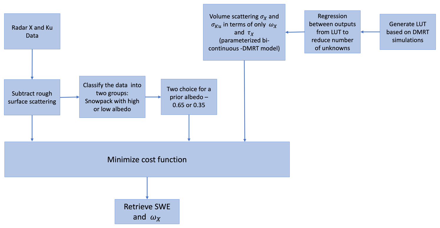
Figure 12 Simplified flow diagram of the algorithm. Two measurements to retrieve two parameters with a prior binary choice of albedo. No prior estimate of SWE.

4.4.1 Steps of retrieval algorithms

• Step 1:​​​​​​​ subtraction of rough surface scattering. The rough surface contributions are subtracted from the radar measurements. The subtraction procedure is as described in Sect. 3.1.2 with several options. We show the case the SnowSAR data collected from the 2013 Canadian TVCExp campaign (King et al., 2018; Zhu et al., 2018) in Fig. 13. SnowSAR flights were performed on 8 and 9 April 2013, crossing each of the TVC sites. The SnowSAR-collected data are shown with purple dots. The bicontinuous-DMRT simulation LUTs are shown with blue dots. The SAR data show a bias when compared with X- and Ku-band DMRT simulations. The bias is attributed to the contributions from surface scattering. Since there are no measurements on the underlying soil in the 2013 Canadian TVCExp campaign, rough surface scattering is determined by differences between radar observations and snow volume scattering calculated based on snow pit measurements. The rough surface bias in the Ku-band data is 1 to 2 dB, while, in the X-band data, the bias is about 4 to 6 dB, which indicates that the surface scattering has more influence at X-band. After subtraction of surface scattering from the SnowSAR data, the resulting SnowSAR data, shown with red dots, are assumed to contain only the volume scattering component. The red dots' volume scattering components of the SnowSAR data fall into the range covered by the bicontinuous-DMRT simulations. The dynamic range of SAR data is also larger with this subtraction.

• Step 2: regression training to reduce number of parameters. Regression training is applied to reduce the number of unknowns (Cui et al., 2016; Zhu et al., 2018, 2021a). Look-up tables (LUTs) are generated based on bicontinuous-DMRT simulations of multiple scattering of snow volume scattering for various snow properties of snow depth, density, and snow microstructure as represented by the ​​​​​​​kc and b parameters in the bicontinuous model. The output-dependent variables for the LUT are backscatter at X and Ku (σ_X and σ_Ku), the effective single-scattering albedo at X and Ku (ω_X and ω_Ku), and optical thickness at X and Ku (τ_X and τ_Ku). Regression training is performed for (i)ω_X versus ω_Ku and (ii) τ_X versus τ_Ku to utilize the frequency dependence of scattering between the X- and Ku-bands.

  In Zhu et al. (2018), there are two trained relations that are derived from regressions. The first regression-trained relation is to train the multiple-scattering solutions into effective first-order solutions, $\mathit{\sigma }=A+B\log \left({\mathit{\sigma }}^{\mathrm{1}\mathrm{st}}\right)$, where σ is multiple volume scattering of snow, and σ^1st is the first-order scattering. The coefficients A and B are given in Zhu et al. (2018) for X- and Ku-bands. In the second regression-trained relation, the relations between albedo at X- and Ku-band and between optical thickness at X- and Ku-band are trained to give ω_Ku(ω_X) and τ_Ku(τ_X). After these two sets of training, we then use ${\mathit{\sigma }}^{\mathrm{1}\mathrm{st}}=\mathrm{0.75}\cos {\mathit{\theta }}_t\mathit{\omega }(\mathrm{1}-\exp (-\mathrm{2}\mathit{\tau }/\cos {\mathit{\theta }}_t\left)\right)$ (Cui et al., 2016; Zhu et al., 2018) and the regression relations, ${\mathit{\sigma }}_{\mathrm{X}}=A_{\mathrm{X}}+B_{\mathrm{X}}\log \left(\mathrm{0.75}\cos {\mathit{\theta }}_t{\mathit{\omega }}_{\mathrm{X}}\right(\mathrm{1}-\exp (-\mathrm{2}{\mathit{\tau }}_{\mathrm{X}}/\cos {\mathit{\theta }}_t)\left)\right)$ and ${\mathit{\sigma }}_{\mathrm{Ku}}=A_{\mathrm{Ku}}+B_{\mathrm{Ku}}\log \left(\mathrm{0.75}\cos {\mathit{\theta }}_t{\mathit{\omega }}_{\mathrm{Ku}}\right({\mathit{\omega }}_{\mathrm{X}}\left)\right(\mathrm{1}-\exp (-\mathrm{2}{\mathit{\tau }}_{\mathrm{Ku}}({\mathit{\tau }}_{\mathrm{X}})/\cos {\mathit{\theta }}_t)\left)\right)$. The results and advantages of this regression training are that the multiple volume scattering at X- and Ku-bands, σ_X and σ_Ku, now only depends on two parameters, ω_X and τ_X. The approach is labeled a “parameterized bicontinuous-DMRT model” (Cui et al., 2016; Zhu et al., 2018, 2021a).

• Step 3: classification of data. Following the strategy of SMAP radar retrieval, classification is performed. We use the dataset from the Canadian SnowSAR 2013 campaign as an example. The a priori information is obtained from co-located ground measurements. The backscattering σ is classified into two groups: snowpack with high albedo and snowpack with low albedo. The threshold ω_X=0.49 is the average of all a priori albedos. Figure 14 shows that the sensitivities of backscatter to SWE are enhanced by classification of snowpack based on a priori scattering albedo. The classification scheme accounts for the heterogeneity of snow cover of varying grain sizes and SSAs from location to location.

• Step 4: a priori estimates, binary choices, and cost function minimization.​​​​​​​ A priori estimates of parameters are applied to determine the mean, the weight, and the uncertainty $\frac{w_{\mathrm{p}}}{\mathrm{2}{s}_{\mathrm{p}}^{\mathrm{2}}}{\left({\mathit{\omega }}_{\mathrm{X}}-{\stackrel{\mathrm{‾}}{\mathit{\omega }}}_{\mathrm{X}}\right)}^{\mathrm{2}}$ of the cost function. A priori information can be obtained from co-located field stations or historical ground measurement data (Rott et al., 2010; Cui et al., 2016; Zhu et al., 2018). In parametrizing microstructure, the snow grain size, correlation length (Proksch et al., 2015a), or scattering albedo (Cui et al., 2016; Zhu et al., 2018) is used.

  In the implementation of Zhu et al. (2018) and (2021a) algorithm, the co-polarization of X-band (9.6 GHz) and Ku-band (17.2 GHz) are utilized in the cost function below.

  $$\begin{array}{}\text{(4)}& \begin{array}{rl}F& =\mathrm{MIN}\left\{{\displaystyle \frac{w_{\mathrm{X}}}{\mathrm{2}{s}_{\mathrm{X}}^{\mathrm{2}}}}{\left({\mathit{\sigma }}_{\mathrm{X},\mathrm{VV}}^{\mathrm{obs}}-{\mathit{\sigma }}_{\mathrm{X},\mathrm{VV}}^{\mathrm{obs},bg}-{\mathit{\sigma }}_{\mathrm{X},\mathrm{VV}}^{\mathrm{model}}\left({\mathit{\tau }}_{\mathrm{X}},{\mathit{\omega }}_{\mathrm{X}}\right)\right)}^{\mathrm{2}}\right.\\ & +{\displaystyle \frac{w_{\mathrm{Ku}}}{\mathrm{2}{s}_{\mathrm{Ku}}^{\mathrm{2}}}}{\left({\mathit{\sigma }}_{\mathrm{Ku},\mathrm{VV}}^{\mathrm{obs}}-{\mathit{\sigma }}_{\mathrm{Ku},\mathrm{VV}}^{\mathrm{obs},bg}-{\mathit{\sigma }}_{\mathrm{Ku},\mathrm{VV}}^{\mathrm{model}}\left({\mathit{\tau }}_{\mathrm{X}},{\mathit{\omega }}_{\mathrm{X}}\right)\right)}^{\mathrm{2}}\\ & \left.+{\displaystyle \frac{w_{\mathrm{p}}}{\mathrm{2}{s}_{\mathrm{p}}^{\mathrm{2}}}}{\left({\mathit{\omega }}_{\mathrm{X}}-{\stackrel{\mathrm{‾}}{\mathit{\omega }}}_{\mathrm{X}}\right)}^{\mathrm{2}}\right\},\end{array}\end{array}$$

  where the two unknown parameters to be retrieved are the scattering albedo at X-band (ω_X) and the optical thickness at X-band (τ_X). The input parameters ${\mathit{\sigma }}_{\mathrm{X},\mathrm{VV}}^{\mathrm{obs}}$ and ${\mathit{\sigma }}_{\mathrm{Ku},\mathrm{VV}}^{\mathrm{obs}}$ are radar observations at X- and Ku-band, ${\mathit{\sigma }}_{\mathrm{X},\mathrm{VV}}^{\mathrm{obs},bg}$ and ${\mathit{\sigma }}_{\mathrm{Ku},\mathrm{VV}}^{\mathrm{obs},bg}$ are background scattering, and ${\stackrel{\mathrm{‾}}{\mathit{\omega }}}_{\mathrm{X}}$ is a priori scattering albedo. In the Zhu et al. (2018) and (2021a) algorithm, ${\stackrel{\mathrm{‾}}{\mathit{\omega }}}_{\mathrm{X}}$ is based on a binary choice. In this minimization problem of the current implementation, there is no a priori estimate of SWE. The only a priori estimate is of the ${\stackrel{\mathrm{‾}}{\mathit{\omega }}}_{\mathrm{X}}$​​​​​​​, and the choice is binary, either 0.65 or 0.35. If better estimation of ${\stackrel{\mathrm{‾}}{\mathit{\omega }}}_{\mathrm{X}}$ can be obtained by ground measurements, snow physical model (Xiong and Shi, 2017), or passive observations (Zhu et al., 2021a), the retrieval performance can be improved. In Eq. (4) w_X, w_Ku, w_p, and s_p are user-defined parameters, while s_Xs_Ku=0.5 dB is an instrument parameter.

  The cost function of Eq. (4) with least squares is applied to the SAR data at X- and Ku-bands in 6. In this example, s_X​​​​​​​ is set to 0.1, and the weight factors are set to be unity We apply the two channel observations to retrieve the two parameters, ω_X and τ_X. Then using retrieved ω_X and τ_X the SWE is obtained by the relation $\mathrm{SWE}=a\left(\mathrm{1}-{\mathit{\omega }}_{\mathrm{X}}\right){\mathit{\tau }}_{\mathrm{X}}$, where a=9745 (Cui et al., 2016; Zhu et al., 2018, 2021a).

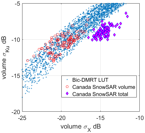
Figure 13 Canadian SnowSAR measurements compared with the bicontinuous-DMRT LUT. Figure from Zhu et al. (2018).

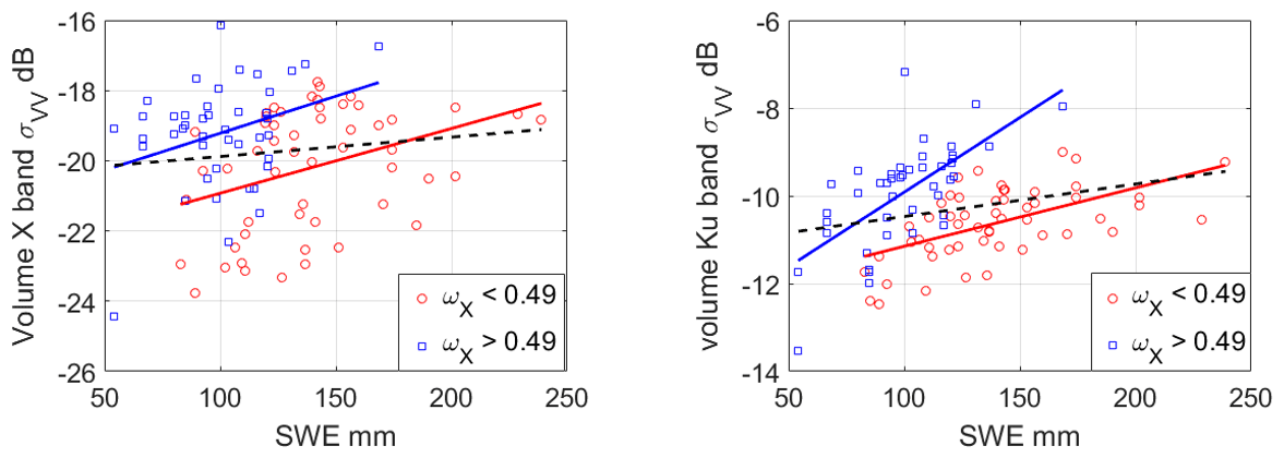
Figure 14 Volume scattering of the Canada SnowSAR data as a function of SWE based on the retrieved scattering albedo ω_X at (a) X-band and (b​​​​​​​) Ku-band. Radar observations are from a single flight. A priori estimates are used to classify ω_X into two classes. They are plotted by different-colored markers. The dashed black curve is the regression line of all Canada SnowSAR data. The solid blue and red curves are the regression lines for backscatter with ω_X larger and smaller than 0.49, respectively. Figure from Zhu et al. (2018).

Figure 15 (a) SWE retrieval performance and (b) scattering albedo retrieval using Canadian SnowSAR 2013 X- and Ku-band radar data. The figures are from Zhu et al. (2018) and Zhu (2021).

4.4.2 Results of retrieval

Figure 15a shows the performance of the retrieval algorithm. The retrieval results have RMSE of ∼ 27 mm of SWE, a correlation of 0.7, and a bias of 6.3 mm. The results show that the retrieval algorithm is particularly successful for SWE values below 150 mm. The performance satisfies requirements from the CoREH2O that the RMSE is less than 30 mm for SWE below 300 mm, and the RMSE is less than 10 % of SWE for SWE above 300 mm. In Fig. 15b, the retrieved scattering albedo ω_X is also shown.

In the equation of cost function, the weight w_X​​​​​​​ is the measure attached to the a priori parameter. In the example of Fig. 15, w_X is set to be 1. In Zhu et al. (2018), we have studied the retrieval performance variation by reducing w_X. The performance is still acceptable down to w_X=0.14 with RMSE equal to 40 mm. Next, we study the performance with variations in surface scattering subtractions by adding noise to the best guess of surface scattering in Zhu et al. (2018). At the best guess with 0 % noise, the RMSE of SWE is 27 mm. The RMSE of SWE retrieval increases with noise increase. However, even with 50 % additional noise (absolute error of 3 dB in surface scattering), the performance has RMSE of 45 mm.

In Fig. 16, we show three-dimensional plots of the σ₀ at Ku-band against the two variables of retrieved scattering albedo and retrieved SWE, along with a three-dimensional fitted plane for two domains: single-scattering albedo >0.49 and <0.49, respectively. The orientation of the two planes indicates that there is a larger dependence on single-scattering albedo for the data with single-scattering albedo >0.49. Thus, the data support the notion that σ₀ is a function of both SWE and single-scattering albedo. On the other hand, Fig. 17 shows the two-dimensional plot of σ₀ against the single variable of retrieved SWE and the two-dimensional fitted line for all of the data. This further illustrates the point shown in Fig. 14: a scatterplot of SWE vs. σ₀ alone is not expected to capture the full relationship between the two variables.

The results show the importance of plotting σ₀ versus two independent variables of SWE and scattering albedo.

Figure 16 Three-dimensional plot of the σ₀ when plotted against two variables at Ku-band (black circles) along with a linear least-squares fits of σ₀ to two variables, SWE and single-scattering albedo (surfaces). The surface color indicates σ₀ value in decibels.

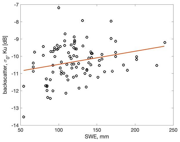
Figure 17 Two-dimensional plot of σ₀ against the single variable of SWE at Ku-band. The line represents a least-squares linear fit between the two variables.

The Zhu et al. (2018) and (2021a) have been applied to a total of seven datasets of airborne and tower measurements, as listed in Tables 2 and 3. The performance of the retrieval algorithms for the seven datasets are summarized in Table 4. The RMSE is generally good.

Table 4 Summary of validations of the dual-frequency algorithm at 9.6 and 17.2 GHz (Zhu et al., 2018, 2021a) against seven datasets of airborne and tower measurements. Details of the seven datasets are listed in Tables 2 and 3.

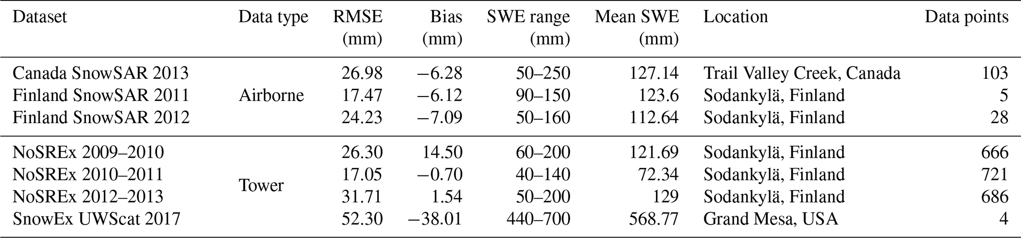
4.4.3 Future work

In the Zhu et al. (2018) algorithm illustrated above, a single layer is used. A multilayer snow model should also be considered. Studies have already been conducted using a two-layer model (King et al., 2018, 2019; Rutter et al., 2019) to account for small grain size in the upper layer and a larger grain size for the bottom layer (depth hoar). Accuracy requirements of a priori estimates to achieve desired retrieval skill have not yet been quantified. Future work should include systematic usage of cross-polarizations in the retrieval algorithms. The inclusion of cross-polarizations is important for deep-snow layers as the co-polarization K-band backscatter saturates for SWE larger than 300 mm. The Ku-band cross-polarization saturation can be shown using bicontinuous DMRT. The data for deep-snow cross-polarization at Ku-band is quite limited.

5 Improving SWE retrieval estimations via synergy with other datasets

In satellite remote sensing, with the vast amount of satellite data, there can be data fusion of synergistic use of other datasets to refine the retrieval algorithms and improve the SWE estimations. Combined active and passive microwave remote sensing using data of the same frequencies has been an active area of research. Recent work shows the use of C-band Sentinel-1 data to retrieve SWE for deep-snow layers. Interferometry and tomography are also studied for future launches of complementary missions. P-band GNSS-R (global navigation satellite system reflectometry) has also been proposed for satellite retrieval of SWE.

5.1 Passive microwave

The GCOM (Global Change Observation Mission) was launched in 2012 and carries the AMSR2 (Advanced Microwave Scanning Radiometer 2) instrument, measuring microwave brightness temperatures at six frequencies. The channels at 18.7 and 36.5 GHz with both V and H polarizations have been used to retrieve global SWE. The spatial resolutions are coarse and are respectively at 22 km by 14 km for 18.7 GHz and 12 km by 7 km for 36.5 GHz. With overlapping footprints, interpolation algorithms have been applied (Long and Brodzik, 2016) to downscale resolution to 3 km. Uncertainty increases when downscaling resolution increases. Because the passive emissivity is related to the radar bistatic scattering (Tsang et al., 1982), the brightness temperatures are related to the radar backscattering cross-sections. Since SAR observations (<500 m) have much finer spatial resolutions than passive radiometry, a synergy is to use SAR at the X- and Ku-bands to downscale coarse-resolution passive data or SWE products (Takala et al., 2011) to finer spatial resolutions using data assimilation or other algorithms.

Several other methods have been explored to combine the active and passive microwave observations to retrieve SWE. In Hallikainen et al. (2003), satellite microwave observations were used to demonstrate its feasibility to retrieve SWE by using passive-only, active–passive, and active-only algorithms in subarctic snow in Finland. Tedesco and Miller (2007) evaluated SWE retrieval performances by using active (Ku-band) and passive (X-band) microwave observations. Recently, Bateni et al. (2015) conducted SWE retrieval studies using passive (Ku- and Ka-bands) and active (L- and Ku-bands) ground-based microwave observations. The SWE retrieval was obtained within a data assimilation framework by comparing simulated microwave observations against the corresponding observations at multiple frequencies.

In the study of Lemmetyinen et al. (2018), the correlation length of snowpack is derived by matching both active and passive microwave observations against the simulations of the MEMLS3&a model (Proksch et al., 2015a) with ancillary data from snow pit measurements and weather stations. Next, the correlation length is used for the active radar algorithm to retrieve SWE. The derived correlation length from both active and passive data demonstrates an improvement of the SWE retrieval performance over the SWE retrieval with the active-only algorithm. Cao and Barros (2020) used a multilayer snow hydrology model coupled to MEMLS3&a to investigate the signature of the variability in snow physics on the microwave behavior at seasonal scales. They found that a combined approach using active microwave sensing in the accumulation season and passive sensing in the melting season would yield the best sensitivity to capture the temporal evolution of seasonal SWE by taking optimal advantage of microwave hysteresis (Ulaby et al., 1981; Kelly and Chang, 2003). The generalization of this approach to available active and passive microwave measurements with a large resolution gap poses a significant challenge.

Recently, passive observations have been used to enhance the performance of the active algorithm (Zhu et al., 2021). The active-only algorithm was described earlier by using a cost function between simulated and observed radar observations as a function of the two parameters of scattering albedo and optical thickness. In this enhancement, passive observations at Ku- and Ka-bands at the collocated and coincident snow scene are used to determine the range of the scattering albedo. The bicontinuous-DMRT model is applied for both passive and active model simulations. X- and Ku-band radar data are then used with the determined scattering albedo to obtain SWE. This active and passive combined method is applied to the NoSREx dataset. Comparison statistics show that the combined active–passive method has improved performance over the active-only method. The retrieval does not require a priori​​​​​​​ information and ancillary data from ground measurements.

5.2 C-band SAR

C-band radar can be used to detect wet snow by the strong decrease in backscatter (Stiles and Ulaby, 1980). Studies have shown contrasting results regarding the potential for SWE and snow depth retrieval, but reviewing the literature on this topic is outside the scope of this paper. We highlight here that some recent studies have demonstrated the possibility of snow depth estimation for deep snow using C-band radar at cross-pol, thus making C-band possibly synergistic with the higher-frequency approaches most applicable to shallower snow depths that are the focus of this paper.

Lievens et al. (2019, 2022) developed an empirical change detection algorithm that was used to estimate snow depth at 1 km spatial resolution from S1 observations over all Northern Hemisphere mountain ranges (Lievens et al., 2019) and, with algorithm improvements, at sub-kilometer resolution over the European Alps (Lievens et al., 2022). The algorithm relies on the ratio of cross- to co-pol backscatter. Here, 300 m retrievals based on the S1 change detection approach are shown for Idaho, Montana, and Wyoming, US. Figure 18a shows a density plot, comparing weekly S1 retrievals for the periods between August and March from 2017 to 2020 with in situ measurements from 203 available SNOTEL sites. Figure 18b shows the MAE relative to the snow depth (in percent), illustrating that for shallow snowpacks (<1 m) the MAE is on average ∼ 50 % with large variance. From 1 m depth onwards, the relative average MAE remains constant at ∼ 30 %. Figure 18c compares time series of snow depth retrievals and measurements for six selected SNOTEL sites. The ESA Sentinel-1 mission is the first C-band radar constellation that measures consistently (not regularly tasked) with the exact same orbit revisited every 6 d. Such a consistent observation scenario benefits the change detection approach and could explain why limited success has been found with other C-band systems that must be tasked. The recent snow depth retrieval results from C-band SAR over mountainous regions with deep snow indicate a strong complementarity with applications at higher frequencies; for example, Ku-band is much more sensitive to shallow snow, while C-band performs better in relative terms for deep snow.

Figure 18 Snow depth retrieval from Sentinel-1, 2017–2020, in Idaho, Montana, and Wyoming. (a) Density plot of weekly 300 m resolution S1 snow depth retrievals and coincident SNOTEL observations from 203 sites. (b) The corresponding mean and standard deviation of the absolute error between S1 retrievals and in situ measurements, stratified by the measured snow depth. (c) Time series comparison between snow depth from S1 and SNOTEL in situ measurements at six locations for three winter seasons. Note that the analysis includes snow-free conditions but excludes wet-snow conditions as detected with the S1 algorithm (Lievens et al., 2022​​​​​​​).

Despite the observational evidence of C-band cross-polarization sensitivity to deep snow, the underlying physical scattering mechanisms and the associated impacts of snow properties are still not fully understood. Snow crystals can form larger-scale clusters that are more similar in size compared to the C-band wavelength. Snow crystals are highly anisotropic (irregular in shape) and, in principle, result in a stronger scattering in cross-polarization. Thus, we would expect that snow microstructure plays a role in governing C-band response to SWE. Other contributions to snow scattering at C-band that can be investigated are larger-scale contrasts in snow density (including between snow layers) and the formation of ice layers with rough boundaries in deep snowpack. Recent progress in snow radiative transfer modeling is addressing the anisotropic shape of snow crystals and the clustering of crystals (Zhu et al., 2021) using a bicontinuous model that introduces a two-parameter correlation function (Ding et al., 2010) and shows that large clustering of grains can cause cross-polarization signals from volume scattering that are in the range observed by S1 and that the volume scattering signal at cross-polarization can dominate over surface scattering for large snow depths. This hypothesized mechanism may explain why cross-polarized C-band radar is sensitive to SWE (Lievens et al., 2019), while co-pol is relatively insensitive to SWE (Naderpour et al., 2022). Further field-based studies of the investigations of the effects of microstructure on C-band radar signals are ongoing. More work is needed to improve our understanding of the physical mechanisms that cause C-band sensitivity to snow mass.

5.3 Phase-based approaches

Approaches to estimating snow characteristics using microwave remote sensing almost invariably make use of some combination of the radar cross-section σ₀​​​​​​​, sensitivity to polarization, and frequency dependence; the techniques previously mentioned are all based on microwave scattering, which focuses on the amplitude response. Approaches that use the signal phase, related to the electrical path length and time-of-flight information, while more challenging, can provide additional information about the snowpack, which is synergistic with the Ku-band backscatter approach that is the focus of this paper. These approaches provide independent information about snow properties through travel time through layers and information about where within the snowpack the major sources of amplitude (e.g., layer boundaries) are originating. The additional information could be used to improve the accuracy of the backscattering retrievals. Three techniques are described: (1) ultra-wideband radar, (2) tomography, and (3) interferometry.

5.3.1 Ultra-wideband radar

The range resolution of a radar system is inversely proportional to the bandwidth. Ultra-wideband radar can be used to resolve reflections from different depths within the snowpack. This not only provides insight into which locations within the snowpack are contributing most to the backscatter but also estimates the depth-dependent refractive index of snow, which can be used to independently estimate snow depth, SWE, and stratigraphy. However, the ultra-wideband radar technology does not have a straightforward path to space due to bandwidth and frequency allocation limitations. Ultra-wideband approaches have been demonstrated for decades from the ground, using broadband radar at nadir incidence angles to estimate depth and SWE (for a review, see Marshall and Koh, 2008), using L-band ground-penetrating radar (GPR) systems (Lundberg et al., 2000; McGrath et al., 2019), and at higher microwave frequencies (Gubler and Hiller, 1984); multi-channel L-band radar has recently been used to map density profiles in polar firn (Meehan et al., 2021). Nadir ultra-wideband FM–CW radar (2–18 GHz) has been flown from an aircraft platform with success in the polar regions as part of NASA Operation IceBridge, mapping snow depth on sea ice and stratigraphy in firn on the ice sheets (Panzer et al., 2013; Arnold et al., 2019). More recently, airborne FM–CW experiments have been done over seasonal snow in the mountains (Yan et al., 2017), with additional efforts being carried out at the University of Alabama in developing airborne tomography mountain applications (Taylor et al., 2020).

5.3.2 Tomography

Recently, synthetic aperture radar (SAR) tomography (TomoSAR) has been used in monitoring the snowpack from X-band to Ku-band (Wiesmann et al., 2019; Rekioua et al., 2017; and Xu et al., 2018, 2020). This technique provides unique access to the structure of the imaged scene, and in the case of snowpack, it enables the separation of multiple snow layers as well as the detection of and compensation for soil and vegetation layers. Polarimetric capabilities can be used to decompose the backscattered signal into volumetric and surface scattering components and to distinguish between snow, soil, and vegetation. Some ground-based field experiments have been carried out that demonstrate the focused image recovery of the layering structure of the snowpack with different densities, for example in a recent experiment (Xu et al., 2018) at Fraser Experimental Forest, Colorado, at X- and Ku-bands (9.6, 13.5, 17.2 GHz). In Fig. 19, we show the results of tomography carried at three frequencies for HH polarization. The tomograms demonstrate the layer structure and frequency dependence. The ability to identify snow layers and density changes are expected to significantly improve SWE retrieval.

Figure 19 TomoSAR coherence images for HH​​​​​​​ polarization at 9.6, 13.5, and 17.2 GHz at Fraser, CO, sites.​​​​​​​

5.3.3 Interferometry

Interferometry can be used to measure differential path length and changes in the electromagnetic path length in signals interacting with the seasonal snowpack. This technique has been proposed in several studies, at both high frequency with single-pass InSAR for mapping the snow surface, to measure snow depth (Moller et al., 2017), and at low frequency with repeat-pass InSAR to measure changes in snow depth or SWE (Guneriussen et al., 2001; Deeb et al., 2011; Lei et al., 2016). Interferometry can be performed either between two observations separated in space (Fig. 20a) or by repeat observations after changes in snow occur (Fig. 20b). Although phase measurements are not absolute measurements (modulo 2π), there are a number of methods, including phase unwrapping, the use of a surface digital elevation model (DEM), and modeled and measured SWE change, that can be used to resolve the ambiguity.

For the first approach (standard cross-track interferometry), using a high microwave frequency or in wet snow where the penetration depth would be limited, we can assume the majority of the signal comes from the snow surface, and the snow surface topography can be mapped. When this is differenced from a snow surface at a different time, a snow depth change can be estimated spatially. This implementation of interferometry is achieved through the introduction in the system of a second antenna separated from the transmitting antenna by the baseline B​​​​​​​. Such an antenna can be passive, receiving the signal of a common transmitter antenna, and the phase difference between the two antennas is measured. The scattering-phase center and the interferometric correlation magnitude can be measured, which are both sensitive to the frequency and polarization combinations as well as the snowpack physical characteristics (e.g., Rott et al., 2021).

In the second approach, a low microwave frequency in dry snow can be used, where we can assume the majority of the signal comes from the snow–ground interface (Fig. 20b). In this case, changes in the time of flight, or electromagnetic path length, to the snow–ground interface are caused by changes in snow depth and SWE. A time series of InSAR observations at L-band can thus potentially be used to estimate changes in snow depth and SWE. This technique was tested during the NASA SnowEx 2020 and 2021 experiments (Marshall et al., 2021). In addition, a similar approach with P-band has been demonstrated from tower-based platforms, using existing transmitted signals (Shah et al., 2017). This bistatic approach shows great promise for a much lower-cost satellite system as only a receiver is required.

Figure 20 (a) Illustration of single-pass InSAR for mapping the snow surface. Using measured phase, Δϕ, simple trigonometric calculations are used to estimate the relative height, h, of the scattering-phase center compared to the reference height, H. (b​​​​​​​) When the phase center is below the snow surface, refraction in snow must also be taken into account. At low microwave frequencies (e.g., L-band) in dry snow, the phase center is often the snow–ground interface, and due to the slower electromagnetic velocity in snow, phase changes are related to changes in snow depth and density.

InSAR has been used for characterizing the volume scattering components of forests (e.g., Kugler et al., 2015), where a vertical profile of the volume density can be estimated (Reigber and Moreira, 2000; Tebaldini and Rocca, 2011). While most of this development has been done at low frequencies for vegetation, a scaling of the volume characteristics of snow with frequency has been equally promising (Lei et al., 2016), especially at Ku- and Ka-band.

In Sect. 6, the planned TSMM mission is described. With the interferometry setup as described in Sect. 5.3.3, we can explore possible configurations, such as the baseline B, of launching a companion satellite with receive-only, receiving the complex scattered electric field signal from the snow medium. Such a companion would be able to complement the planned baseline TSMM observations with additional measures of reflectivity, interferometric phase, and correlation magnitude that could all be used to better characterize the snow volume.

6 Planning a satellite mission

The earliest synthetic aperture radar (SAR) satellite missions were focused on C-band (ERS-1, Radarsat-1). Missions developed during recent decades extended the frequency range to L- (e.g., PALSAR) and X-band (e.g., TERRASAR-X), with planned missions at the P- (ESA-Biomass), L- and, S-bands (NASA-ISRO SAR mission). Spaceborne scatterometer missions such as QuikScat have illustrated the wide-ranging contributions of measurements at Ku-band to applications spanning the cryosphere (Kwok, 2007; Swan and Long, 2012), biosphere (Frolking et al., 2006), and ocean (Bourassa and McBeth, 2010​​​​​​​). Ku-band cloud radar measurements have made significant contributions to precipitation-related fields through missions like CloudSat (Stephens et al., 2002) and GPM (Skofronick-Jackson et al., 2017).

The potential for Ku-band radar to retrieve snow water equivalent (SWE) was explored as part of the NASA Snow and Cold Land Processes Mission and supporting Cold Land Processes Experiment (Yueh et al., 2009; Cline et al., 2009). The ESA COld REgions Hydrology High-resolution Observatory (CoReH₂O; X- and Ku-bands; Rott et al., 2010; ESA et al., 2012) completed Phase A in 2013 but was not selected for implementation. CLPX and CoReH₂O science and mission development activities played a major role in motivating the significant progress achieved over the past decade in measuring, understanding, and modeling the Ku-band radar response to SWE, snow microstructure, and snow wet/dry state (as assessed in previous sections of this review). Given this collective progress, satellite mission concept reviews following the completion of CoReH₂O Phase A further emphasized the potential for Ku-band SAR measurements to address a broad set of user requirements related to seasonal snow mass.

Supported by these studies and continued analysis of experimental ground-based and airborne campaigns (see Sect. 4; King et al., 2018; Lemmetyinen et al., 2018; Zhu et al., 2018), a Ku-band SAR mission was selected as the most feasible approach to meet the operational requirements (wide swath, rapid revisit, short latency) of Environment and Climate Change Canada (ECCC) for spaceborne measurements sensitive to SWE. Since 2018, ECCC and the Canadian Space Agency (CSA) have partnered to advance the scientific and technical readiness of the “Terrestrial Snow Mass Mission” (TSMM), a Ku-band radar satellite with the primary science objectives focused on the provision of climate services related to seasonal snow and improved operational environmental prediction including streamflow. The TSMM development effort is underpinned by engagement with Canadian industry, academia, and international partners.

Table 5 Summary of CoReH₂O and TSMM missions.

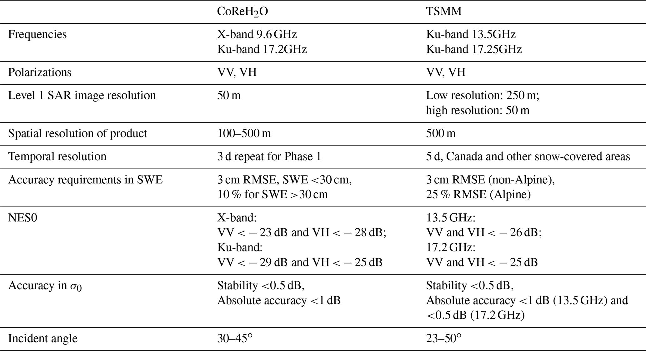
Because TSMM is the first spaceborne Ku-band SAR mission of its type, an “Explorer” mission concept was developed by industrial partners in Canada to advance technological innovation and prove the scientific viability using a “design-to-cost” approach. The resulting “TSMM-Explorer” concept meets ECCC science requirements through dual-frequency (13.5 and 17.25 GHz) Ku-band radar measurements at 500 m spatial resolution, with a 50 m spatial resolution mode across a 30 km swath available for specific regions (e.g., mountains areas) and targeted events (e.g., periods of high flood risk). An imaging swath of 250 km combined with a duty cycle of approximately 25 % meets the requirement to image all of Canada and other global snow-covered areas every 7 d.

In the CoReH₂O proposal, the dual frequencies were in the X-band at 9.6 GHz and the Ku-band at 17.2 GHz. The theoretical predictions of rough surface scattering at X-band, depending on penetration through the snow layer, are from −20 to −12 dB. In TSMM, the X-band (9.6 GHz) is not chosen and is replaced by a low Ku-band at 13.5 GHz.

Table 8 shows a comparison between CoREH2O and the current TSMM concept. The TSMM frequencies were selected to fully exploit the frequency dependence of snow volume scattering through the differential sensitivities at 13.5 and 17.25 GHz to both SWE and snow microstructure. The dual frequencies will help address the ill-posed nature of retrieving SWE from a single Ku-band radar measurement (see Sect. 4.2.2​​​​​​​). The change in the lower frequency of CoReH₂O (9.6 GHz) to TSMM (13.5 GHz) will result in less sensitivity to the underlying rough surface scattering effect, but sensitivity to deep snow will be reduced without the X-band measurement. Further study is needed in fine-grained mountain snowpacks to better understand the limits of sensitivity to deep snow at Ku-band.

The approach to optimally integrate spaceborne radar measurements with state-of-the-art modeling systems is currently under development at ECCC. For applications which require a SWE retrieval, the radar backscatter measurements will be combined with snow property initial conditions (including snow microstructure; see Sect. 4) produced by an advanced version of the ECCC operational land surface model forced with short-range meteorological forecasts and precipitation analyses. Importantly, in areas without radar coverage (e.g., due to swath gaps) or where the radar-derived SWE retrieval is highly uncertain (e.g., due to wet snow or dense forest cover), the SWE analyses will be determined by numerical outputs from the land surface model. In this way, the remote sensing information is combined with modeling to create seamless coverage in both space and time, with minimized uncertainty. Another goal is to assimilate the Ku-band radar measurements directly in ECCC prediction systems without a SWE retrieval. For land surface data assimilation needs, the Ku-band backscatter will be directly assimilated, again with the land surface model providing the required ancillary information. This approach is analogous to how L-band radiometer measurements from the SMOS and SMAP missions have improved soil moisture analysis at ECCC through radiance-based assimilation (Carrera et al., 2019). Work remains to fully implement a forward radar model coupled with the physical snow model, building on recent developments in this field (Bateni et al., 2015; Merkouriadi et al., 2021).

While the dual-frequency Ku-band TSMM-Explorer concept meets the requirements at ECCC for enhanced snow remote sensing, this approach alone cannot solve all snow-related observational needs. For instance, volume scattering will be negligible under wet-snow conditions, hence the need to implement the approach outlined above to combine satellite- and model-derived information during snowmelt. There are, however, opportunities to further exploit the baseline TSMM-Explorer concept through the development of companion satellites. This could take the form of a similar mission concept to improve coverage and revisit (e.g., a small SAR constellation). Development of a companion receive-only satellite is more challenging but would deliver a greater reward through the potential for InSAR-based snow depth retrievals under wet-snow conditions (as previously explored with airborne Ka-band measurements by Moller et al., 2017). This InSAR approach, as described in Sect. 5.3, necessitates pushing the performance envelope of the TSMM-Explorer SAR (bandwidth, increased high-resolution-mode imaging) and spacecraft (maintenance of a very tight baseline, hence very precise orbit control), which introduces cost and complexity to the current scope of the mission. Still, the potential benefits of an InSAR capability are notable, so further study of these options is encouraged.

With the industrial Phase 0 now complete, the TSMM-Explorer mission has advanced into a mission planning phase at CSA. Technical readiness is being advanced through industrial investment focused on the radar antenna technologies. Scientific readiness for the mission continues to be enhanced by community-wide progress in field techniques (e.g., quantitative snow microstructure measurements; Sect. 3.3), physical snow modeling (Sect. 4.2), data assimilation, and multi-frequency radar analysis (Sect. 4.4). The analysis of tower and airborne Ku-band radar datasets in collaboration with international partners is ongoing. Future airborne data acquisition plans are under development, including through the NASA SnowEx program. Collectively, these efforts serve to advance the TSMM-Explorer mission specifically and snow–radar science in general.

7 Summary and perspectives

Fresh water delivered by seasonal snowmelt is a commodity of utmost importance for human health and well-being, supports many sectors of the economy, sustains ecosystems, and poses risks by contributing to floods and sustaining drought events (Barnett et al., 2005; Li et al., 2017; Qin et al., 2020). At present, information on water stored as seasonal snow is highly uncertain. Because of surface monitoring limitations, satellite measurements are critical, but current missions are inappropriate for determining snow mass with the spatial, temporal, and accuracy characteristics required to deliver climate services, effective water resource management, and skillful environmental prediction such as streamflow.

Over the last decade, X- and Ku-band radar remote sensing technologies have shown clear potential for monitoring SWE. Scattering models now provide understanding of the contributions of volume and surface scattering and the complicating effects of forests. Snow physical models have significantly advanced and are capable of providing the required snow microstructure information required for forward and inverse modeling. Tower and airborne radar measurements, supported by dramatic improvements in field-based quantitative characterization of snow microstructure, have provided a small but rapidly growing range of datasets to support modeling and retrieval studies. In the coming years, there is a clear need for more experimental measurement campaigns to fill information gaps (such as the influence of vegetation and sensitivity to deep snow) and evaluate new SWE retrieval frameworks. There will be more studies on coupling snow physical models to radiative transfer models so that they can be more effectively combined in retrieval algorithms with computational efficiency for real-time retrievals.

We anticipate the continued development of satellite missions with Ku-band radars, which could be followed by synergistic instruments supporting techniques such as Ku-band interferometry and tomography.

Appendix A: Example protocol for measuring spatial variability in snow properties to support radar remote sensing

Geolocated measurements are vital to quantify variability in snowpack properties within sensor footprints (airborne or tower). Figure A1a suggests an optimal configuration of snow depth and snow micropenetrometer (SMP) measurements to create representative distributions of snowpack properties within airborne swaths. The main 222 m transect of snow depth and SMP profiles, located along an airborne swath centerline, has variable spacing (10⁻¹, 10⁰, and 10¹ m) on either side of a central pit to capture different horizontal length scales of variability. A shorter 22 m orthogonal transect with 10⁻¹ and 10⁰ m spacing bisects the main transect at the central pit, and a spiral of snow depths extends from the central pit out to an 11 m radius (Fig. A1a). Measurements additional to the main transect allow omnidirectional analysis of snow depth variability and bi-directional analysis of snow microstructural properties, both of which may be influenced by dominant prevailing wind direction or irregular patterns of subnivean vegetation. Ideally, snow depths and positions are measured using automatic depth probes with integrated GPS providing position accuracy to ±2.5 m, e.g., Magnaprobes (Sturm and Holmgren, 2018). Where forest canopies obscure GPS satellite connection, or snowpacks are deeper than 180 cm (current maximum Magnaprobe length), hand probes are used in measured grids arranged relative to a known absolute position. Accuracy of snow depths range from nearly 0 cm on hard ground to ∼ 5 cm in soft subnivean vegetation. Where snow pit locations are not predetermined, measured snow depth distributions can be subsequently used to determine the location of snow pit(s) to match mean depth or multiple pits spanning interquartile ranges.

One-dimensional (vertical) measurement of snowpack properties for SAR retrievals requires objective measurements of snow microstructure. SMP allows rapid (<1 min) force profile detection at millimeter resolution (Proksch et al., 2015b), which is used to derive density, correlation length, and specific surface area (SSA), quantities directly or indirectly used by radiative transfer models (Chang et al., 2016; Picard et al., 2018). The speed of data acquisition allows for SMP measurements to be used in a distributed manner along transects, but SMP also supports other coincident snow pit measurements using different techniques. Figure A1b shows a schematic of optimal snow pit measurements. Double-sampled volumetric density measurements, 100 cm³ box cutter with 3 cm vertical resolution for shallow snowpacks or 1000 cm³ wedge cutter with 10 cm vertical resolution for deep snowpacks (Proksch et al., 2016), are averaged at each vertical position. Following principles presented in Gallet et al. (2009), 3 cm vertical resolution double-sampled SSA measurements are made using an infrared integrating sphere (IRIS) (Montpetit et al., 2012) or an A2 Photonic Sensors IceCube (Zuanon, 2013). µ-CT analysis of snow casts (Schneebeli and Sokratov, 2004; Lundy et al., 2002), consisting of entire profiles or samples of critical layers, are used as a benchmark for corroboration of all other measurements. However, in practice, in situ snow casting and subsequent cold-laboratory µ-CT analysis require a much higher level of expertise and processing time than SMP or IRIS/IceCube measurements, meaning field application of µ-CT is often limited.

Profiles of snow temperature using well-calibrated stem thermometers at 10 cm vertical resolution are important parameters for radiative transfer models, in conjunction with stratigraphic identification of snow layer boundaries and ice lenses using hand hardness. Visual identification of grain type (Fierz et al., 2009) using a hand lens or macroscope is an important complementary measurement for layer classification and understanding the seasonal history of snowpack processes. However, similar visual methods to quantify snow “grain size” are too subjective to create a microstructural metric for further use in radiative transfer models. The SSA measurements provide much better accuracy for use in radiative transfer models.

Near-infrared (NIR) photography allows two-dimensional analysis of layer boundary position (Tape et al., 2010) and layer thickness variability (Rutter et al., 2019) in snow trenches, quantifying spatial variability in stratigraphy around a single snow pit profile. It also enables measurements of layer boundary roughness, particularly of the snow–air and snow–ground interfaces. Other methods to characterize snow–air surface roughness use photographic image contrast analysis of dark boards placed behind snow (Fassnacht et al., 2009; Anttila et al., 2014) and subnivean roughness of areas cleared of snow using pin profilers, lidar scanning (Chabot et al., 2018; Roy et al., 2018), or structure from motion photogrammetry (Meloche et al., 2020). The subnivean roughness between snow and soil gives significant contributions of rough surface scattering because of the contrast of dielectric constants between snow and soil.

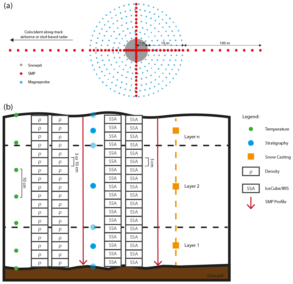
Figure A1 Optimal measurement configurations for evaluation of snow properties in sensor footprints.

Appendix B: Abbreviations

AIEM	Advanced Integral Equation Model
Can-CSI	Canadian CoReH2O Snow and Ice Experiment
CASIX	Canadian Snow and Ice Experiment
CF	Coniferous forest
CMIP6	Coupled Model Intercomparison Project
CoReH2O	Cold Regions Hydrology Observatory
DMRT	Dense Medium Radiative Transfer
DMRT-ML	Dense Medium Radiative Transfer – Multiple Layers
EM	Electromagnetic
ESA	European Space Agency
FMCW	Frequency-modulated, continuous-wave
GNSS-R	Global navigation satellite system reflectometry
HUT	Helsinki University of Technology
InSAR	Interferometric SAR
Lidar	Light detection and ranging
LUT	Look-up table
LWC	Liquid water content
MEMLS	Microwave Emission Model of Layered Snowpacks
MIMICS	Michigan Microwave Canopy Scattering
NMM3D	Numerical solutions of Maxwell's equations in 3-D
NoSREx	Nordic Snow Radar Experiment
NWP	Numerical weather prediction
PolSCAT	Polarimetric Ku-Band Scatterometer
QCA	Quasi-crystalline approximation
SAR	Synthetic aperture radar
SMAP	Soil Moisture Active and Passive
SMOS	Soil Moisture and Ocean Salinity
SMP	Snow micropenetrometer
SMRT	Snow Microwave Radiative Transfer
SSA	Specific surface area
SWE	Snow water equivalent
SWESARR	Snow Water Equivalent SAR and Radiometer
RTE	Radiative transfer equation
RTM	Radiative transfer model
UAVSAR	Uninhabited Aerial Vehicle Synthetic Aperture Radar
µ-CT	Micro-computed tomography