Thickness of multi-year sea ice on the northern Canadian polar shelf: a second look after 40 years

This paper presents a systematic record of multi-year sea-ice thickness on the northern Canadian polar shelf, measured during the autumn and early winter of 2009–2010. The data were acquired by submerged sonar moored in the Penny Strait where they measured floes drifting south from the notional “last ice area” until 10 December, when the ice stopped moving for the remainder of the winter. Old ice comprised about half of the 1669 km long survey. The average thickness of old ice within 25 km segments of the survey track was 3–4 m; maximum keels were 12–16 m deep. Floes with high average draft were of two types, one with interspersed low draft intervals and one without. The presence or absence of thin patches apparently distinguished large floes formed via the aggregation of smaller floes of various ages and deformation states from those of a more homogeneous age and deformation state. The former were larger and of somewhat lower mean thickness (1–5 km; 3.5–4.5 m) than the latter (400–600 m; 6.5–14 m). A calculated accretion of new ice onto the multi-year floes measured in the autumn of 2009 was used to seasonally adjust the observations to thicknesses expected by late winter, when comparative data were acquired in the 1970s. The adjusted mean thickness for all 25 km segments with $\mathrm{4}/\mathrm{10}$ or more old ice was 3.8 m (sample deviation of 0.5 m), a value indistinguishable within sampling error from values measured in the up-drift area during the 1970s. The recently measured ice-draft distributions were also very similar to those from the 1970s. These results suggest that the dynamical processes that create very thick multi-year ice via ridging close to the study area have been less influenced by climate change than the thermodynamic processes behind the formation and decay of thinner level floes. The hazards posed by such ice therefore persist regionally, although the risk has decreased with the decrease in old-ice concentration during recent decades.

1 Introduction

Bourke and Garrett (1987) prepared the first compilation of sea-ice-draft (viz. thickness) surveys in the Arctic Ocean. Their map showed clearly the progressive increase in the average draft of sea ice from 1–2 m on the Siberian side of the Arctic to more than 6 m at some places near the northern coastlines of Greenland and the Canadian Arctic Archipelago. This spatial pattern of ice thickness in the Arctic has been attributed to the combined influences of the long freezing and short thawing seasons at high latitude (Maykut and Untersteiner, 1971) and of pack-ice convergence onto these windward shorelines (Tucker et al., 1979); the convergence maintains high ice concentration and enhances the formation of thick ice rubble via material failure under pressure (Kovacs, 1972).

A compact area of multi-year sea ice has persisted on the North American side of the Arctic during the last quarter century while the area covered by multi-year ice in the Arctic Ocean has decreased considerably (e.g. Comiso, 2012; Kwok, 2018; Stroeve and Notz, 2018). Moreover the numerical models informing the Sixth Assessment Report of the IPCC suggest that the same geographic distribution will continue into the future (e.g. Ridley and Blockley, 2018, their Fig. 2). This evidence has fostered the concept of a future remnant “last ice area” over and adjacent to the north Greenland and Canadian polar shelves (Pfirman and Tremblay, 2009; Pfirman et al., 2010; Hamilton et al., 2014); this area is thought to be ecologically important as a future refugium for ice-reliant Arctic wildlife from bacteria to megafauna (http://www.wwf.ca/conservation/arctic/lia/, last access: 29 July 2022).

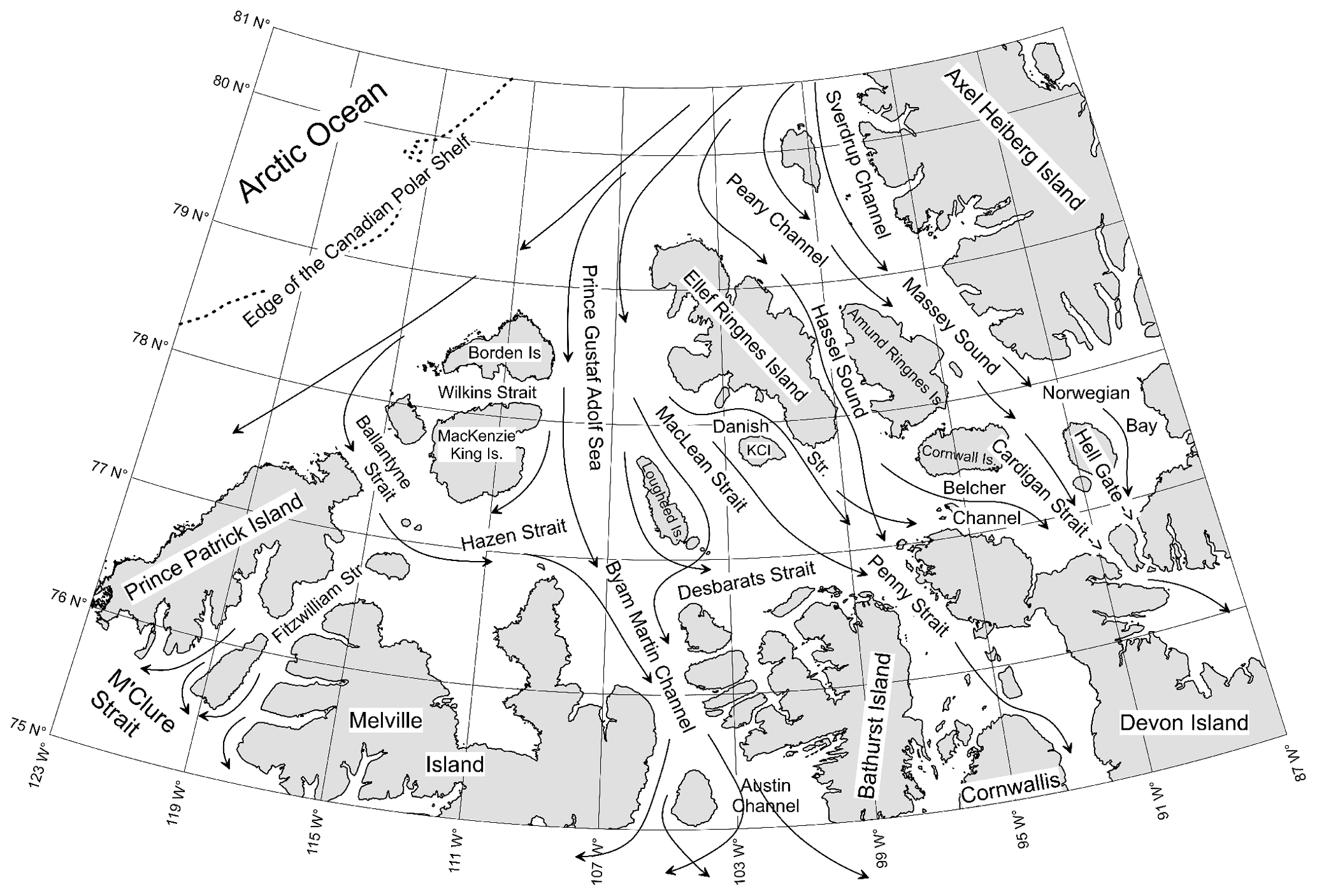
Figure 1 The northern part of the Canadian polar shelf, its principal geographic features and the schematic pattern of sea-ice movement across it. The map encompasses the Queen Elizabeth Islands which overly the feature known to geologists as the Sverdrup (sedimentary) Basin.

Although clearly of concern, the notion of a threatened last area of ice, now rapidly thinning, is based on remarkably few data from that area, past or present (Lyon, 1984; Melling, 2002; Lindsay and Schweiger, 2015). In the compilation by Lindsay and Schweiger (2015) of Arctic ice-thickness observations acquired since 1975, there are points since 2003 that lie within the northwest part of the area of most persistent ice, but unfortunately this region lacks comparative data from earlier times. Moreover the recent data from this area are best viewed cautiously: they are estimates over the 20–70 m diameter footprint of a satellite altimeter that is large relative to ice and snow surficial features; estimates are further compromised by the scarcity of snow-depth and sea-level-height data and by minimal in situ validation (Kwok et al., 2020).

Information on sea ice is also sparse within the adjacent part of the notional last ice area that overlies the Sverdrup Basin – geologists' shorthand for the northern Canadian polar shelf. The extent of ice here and its composition by ice type have been monitored and charted by the Canadian Ice Service since about 1970 to provide guidance for navigation during August and September. The drift of ice through the area has been determined sporadically by following identifiable floes in satellite images and by satellite tracking of beacons on floes that fortuitously entered the area. Knowledge of ice thickness is based almost entirely on borehole measurements, weekly single-point values near Canadian weather stations since the 1950s and transects of borehole measurements acquired during on-ice seismic surveys in the 1970s (Melling, 2002). In addition there have been a few targeted surveys of extreme features, documented in Melling (2002).

More recent studies of ice in this area have been focused on ice kinematics and concentration, including fast ice (Galley et al., 2012), systematic estimates of ice inflow from the Arctic Ocean via feature tracking in satellite images (Alt et al., 2006; Kwok, 2006; Agnew et al., 2008; Wohlleben et al., 2013; Howell and Brady, 2019), decadal fluctuations in multi-year-ice concentration (Howell et al., 2008, 2010, 2013, 2015; Tivy et al., 2011) and summertime deterioration of multi-year floes in the area (Dumas et al., 2007; Howell et al., 2009).

Figure 1 depicts the northern part of the Canadian polar shelf, annotated with the names of its larger islands and waterways. This basin is an area of consistently high ice concentration, with old ice comprising 85 %–90 % of the ice present, except in the area north of Bathurst Island (70 %) and in Norwegian Bay (50 %) (Melling, 2002). Some of this ice enters from the Arctic Ocean in the northwest during the few months of mobility in late summer and autumn; this ice tends to be highly deformed and extremely thick. A second population develops within the basin from areas of first-year ice that do not melt during the brief summer (Flato and Brown, 1996). All ice drifts generally southward to the Northwest Passage, entering this waterway chiefly via the Byam Martin Channel, Penny Strait and Cardigan Strait in the lower right quadrant of the map. These channels draw ice from the Arctic Ocean principally at four entry points, the Sverdrup Channel, Peary Channel, Prince Gustaf Adolf Sea and Ballantyne Strait, with a combined width of 314 km. Ice exits these channels variously via the Hazen, Maclean or Desbarats straits or Hassel or Massey sounds. Although ice drifts quite slowly along these pathways, it moves faster through the narrower exits to the Parry Channel (combined width of 76 km), averaging about 15 km d⁻¹ within the Penny Strait (Fig. 6). A typical journey across the basin in past times has taken 3–5 years because the ice was land-fast between the High Arctic islands for up to 10 months per year. The number of years taken to cross the basin varies with conditions of ice congestion, wind and temperature in summer and appears to have decreased during the last 1–2 decades (Howell and Brady, 2019).

The average thickness of sea ice tends to decrease towards the southeast. In the 1970s, survey-line means as high as 5–7 m were measured near the northwestern margin of the polar shelf and as high as 3–4 m near the exits to the Northwest Passage (Fig. 2). Melling (2002) proposed that the cause of this progressive thinning with distance from the outer shelf was a small sustained heat flow to the ice from the ocean, a mechanism that has been further documented by Melling et al. (2015).

We do know that there were appreciable reductions in the multi-year-ice coverage of the northern polar shelf in 1961, 1970–1971, 1979–1981, 1983–1985, 1997–1999, 2005–2007, 2011–2012, 2014–2015 and 2019 (Dumas et al., 2007; Howell et al., 2010; https://iceweb1.cis.ec.gc.ca/IceGraph/page1.xhtml?lang=_en, last access: 29 July 2022). It has been typical of multi-year-ice coverage to return to historical values within a few years of each such event, via recruitment of second-year ice from remaining first-year ice and via inward drift of old ice from the Arctic Ocean (Howell et al., 2015). However a reduced presence of multi-year ice in this area since the early 2000s has been noted by Howell and Brady (2019).

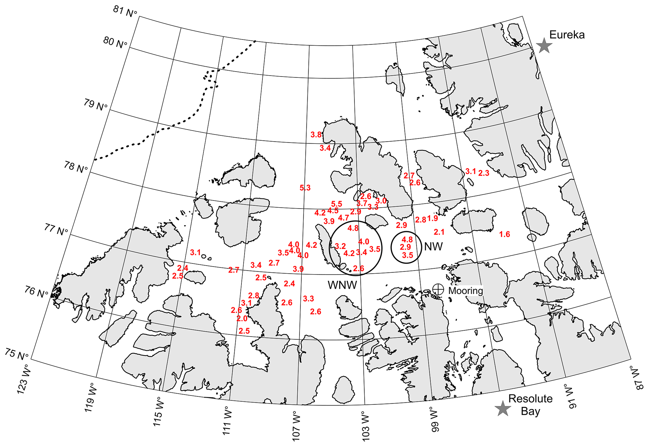
Figure 2 Mean thickness of sea ice in late winter, 1971–1980, derived from holes drilled during seismic surveys (Melling, 2002). Each value is the average from a median of 1835 boreholes, spaced at least 110 yd (100.6 m) apart on a 2D survey grid. Values used in reference to 2009 data are circled. Climate stations and the 2009–2010 mooring site are indicated.

Future severe ice conditions on the Canadian polar shelf are critically dependent on whether all multi-year ice disappears from adjacent areas of the Arctic Ocean; the ice regime of the Sverdrup Basin would be very different if the inflow of heavy ice from the northwest were to cease. It is useful to note that paleo-climatic indicators reveal that there was heavy ice in this area in summer even during the Holocene warm period, 5000 years ago (Dyke et al., 1996; Dyke and England, 2003), when the Arctic climate was 2–3 ^∘C warmer than that during the 20th century.

The thickness of multi-year ice presently over the northern polar shelf is not known; there have been no observations since the late 1970s. However over the southern part of the polar shelf, Haas and Howell (2015) measured multi-year ice in the late winters of 2011 and 2015 using an airborne electromagnetic sensor; they observed expanses of ice averaging 3–4 m over tens of kilometres in the Byam Martin Channel, southern Viscount Melville Sound and the southern M'Clintock Channel, noting that “features more than 100 m wide and thicker than 4 m occurred frequently”.

Acknowledging the much reduced thickness and extent of multi-year ice in the central Arctic (Lindsay and Schweiger, 2015; Stroeve and Notz, 2018), one might anticipate that multi-year ice over the northern polar shelf may also have thinned dramatically. If so, the feasibility of marine transport through the Northwest Passage and across the Sverdrup Basin and of developing proven local natural gas reserves may have increased. Severe ice conditions here in the 1970s were one of the factors driving the shelving of these gas fields at that time.

There is also motivation from the perspective of ice dynamics. A range of factors appear to have influenced recent ice loss from the central Arctic – the pattern of ice circulation, reduced residence time, albedo feedback, warming ocean, warming atmosphere and poorer recruitment of second-year ice. The seas of the Canadian High Arctic are relatively isolated from the Canada Basin, but they do harbour some of the heaviest multi-year ice in the Arctic. Study of ice here, where gain and loss factors for sea ice may be different, could provide new perspectives on sea ice and climate change.

The goal of this study was a timely second assessment of ice within the notional last ice area. Perhaps paradoxically, we chose not to work in the area itself but rather to observe ice as it was leaving via channels along its southern margin. The reason, as is common in Arctic field science, was logistical. Access to the interior of the Sverdrup Basin would have been very costly by icebreaker and perhaps not practical even in summer. Use of aircraft in winter would have been cheaper but contingent on the presence of first-year ice suitable for landing ski-planes, which is scarce here. These factors provided a strong motivation for making observations at the most southerly useful locations. We chose the Penny Strait for the first year of observation. Comparable data have since been collected elsewhere along the margin of the last ice area, in the Byam Martin Channel and in the Nares Strait. Because inter-annual variation was likely to be appreciable, we sustained observations in these channels for several years.

2 Year-round ice monitoring in the Penny Strait, 2009–2010

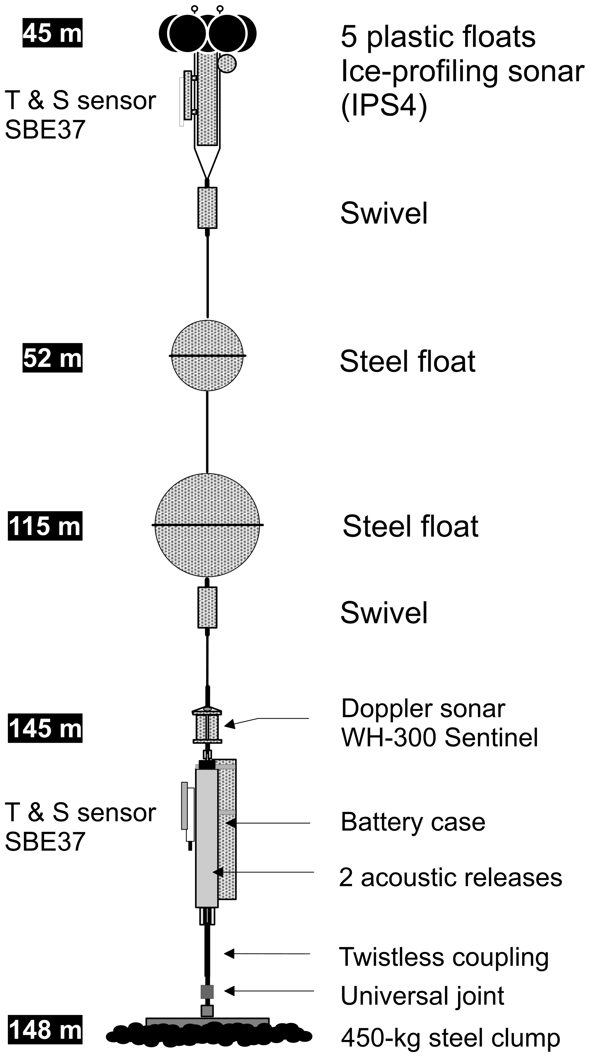
Figure 3 Mooring used to support sonar in the Penny Strait. The twistless coupling enables measurement of ice-drift direction.

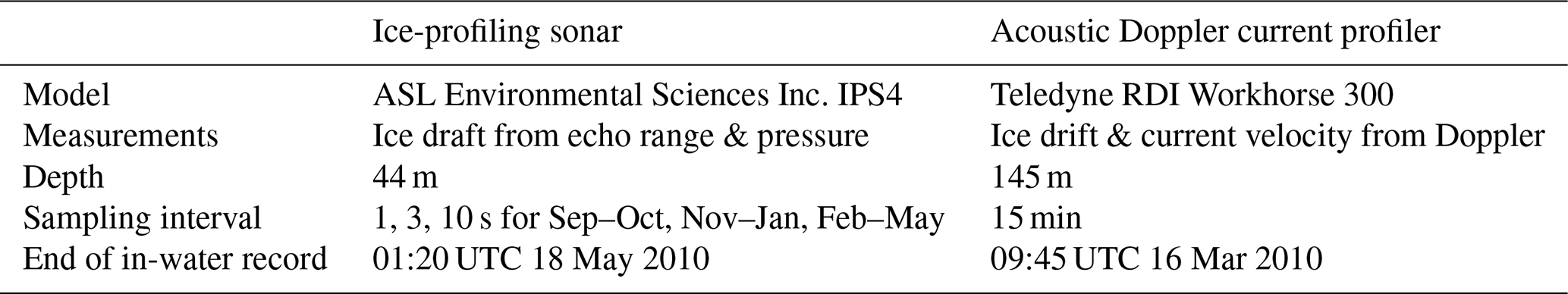
Drilling or electromagnetic induction radar (Haas et al., 2009) can provide ice-thickness transects at good (∼ 25 m) spatial resolution but require human presence; these methods are impractical for year-round sea-ice observation at isolated locations. We used an optimally designed ice-profiling sonar (IPS) for measuring under-ice topographic profiles, capable of operating autonomously for 3 years (Melling et al., 1995). Moored at a fixed location, it measures the submerged depth of ice (draft) as the difference between the depth of the instrument (from a pressure measurement) and its distance from the ice bottom (from an echo). The IPS is used in combination with acoustic Doppler current profiler (ADCP) sonar which measures ice-drift velocity; together the instruments provide data from which a detailed topographic transect of pack-ice floes, ridge keels and leads can be constructed. The spatial separation of survey points is proportional to ice-drift speed, so when ice becomes immobile the IPS is limited to measuring the slow local growth and decay of ice stalled above it.

These instruments were placed on a submerged mooring (Fig. 3) with the ADCP near the seabed and the IPS at 45 m depth, where it was safe from deep ice keels. Because there is no suitable geomagnetic reference for ice-drift direction at this location – the geomagnetic inclination was 88.3^∘ – the section of the mooring beneath the ADCP was torsionally rigid (i.e. no twisting). All ice-drift measurements by the ADCP were made relative to its fixed, albeit unknown, heading that was later deduced during the processing of data using the directions of measured tidal currents. This method has been used successfully since 1998 for oceanographic moorings in the Cardigan Strait, Hell Gate and the Nares Strait (Münchow and Melling, 2008).

The mooring was placed on the southwestern side of the Penny Strait in order to measure multi-year ice leaving the northern polar shelf. This outflow is manifest as a persistent tongue of $\mathrm{4}/\mathrm{10}$ to $\mathrm{9}/\mathrm{10}$ pack ice hugging the southwestern shore in the late summer and autumn (Melling, 2002, their Fig. 3).

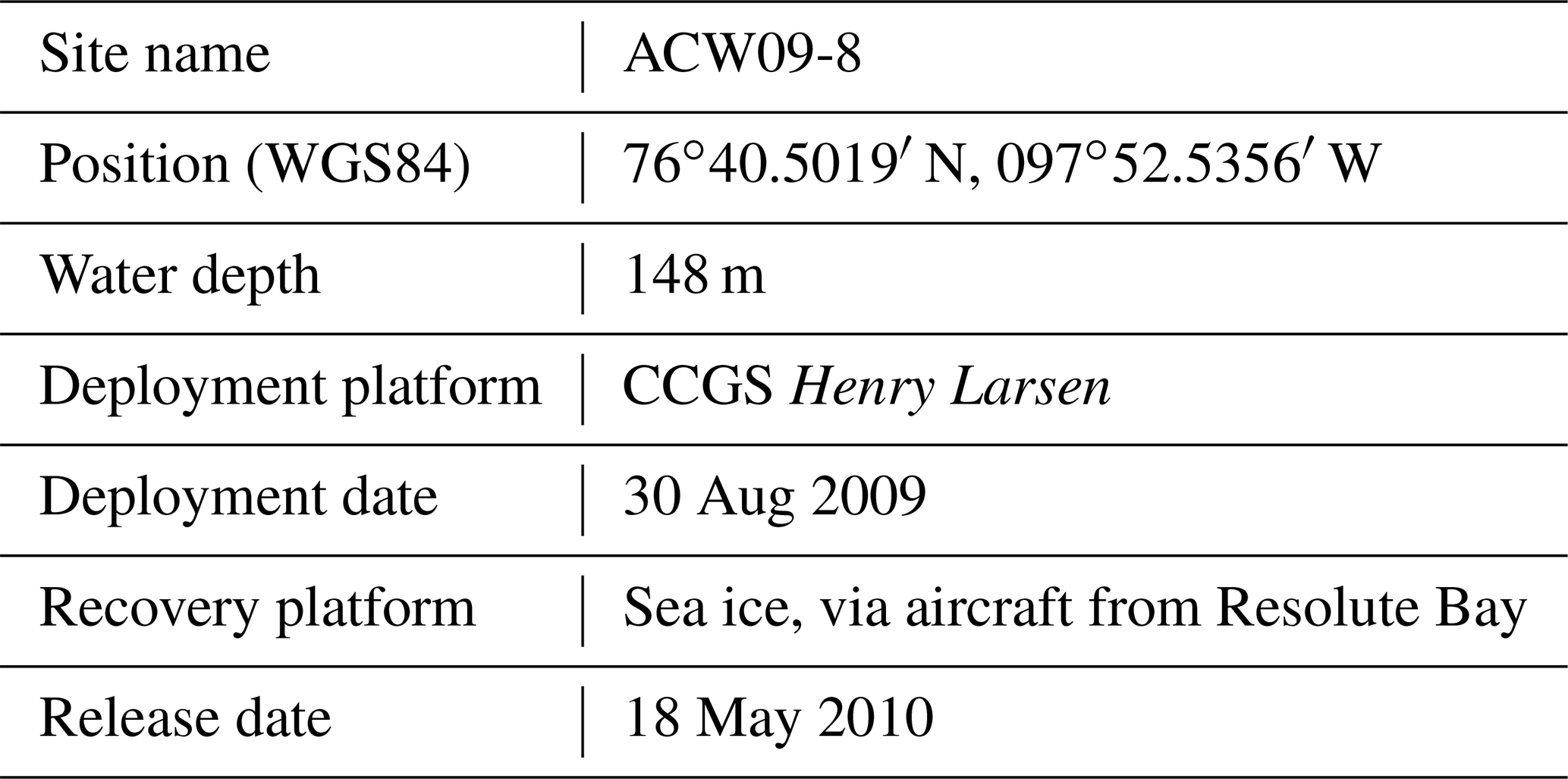
Ironically these same streams pose challenges for the deployment and recovery of moorings. We were able to deploy our mooring from an icebreaker (CCGS Henry Larsen) within this fast-moving heavy ice. However for recovery, the ship needs to reach and hold station at the pre-determined location of the mooring, requirements that would have been difficult under the conditions encountered at deployment. We retrieved the mooring in late May 2010, operating from the surface of fast ice accessed by aircraft. Details of the data collection are summarized in Tables 1 and 2.

Table 1 Oceanographic mooring in the Penny Strait.

Table 2 Ice-measuring instruments on the Penny Strait mooring.

3 Observations

3.1 Environmental conditions during the period of observation

Figure 4 is a radar satellite view of the Penny Strait just before the ship's arrival in 2009; it clearly shows a dense stream of multi-year floes drifting down from the north at this time. When the ship reached the site of the installation, a team from Canada's National Research Council completed a borehole survey on one of the floes nearby; as reported by Johnston (2019), the minimum borehole thickness from 20 drillings of this floe, 1500 m across, was 8.4 m and the median was 16.1 m.

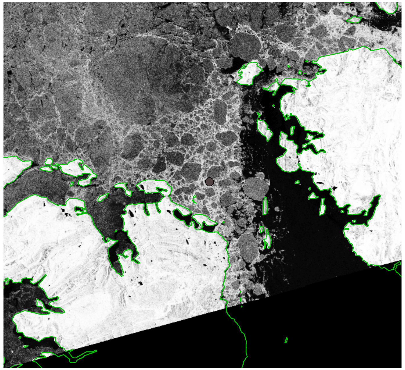
Figure 4 Multi-year pack ice in the Penny Strait on 23 August 2009. Ice-free water appears dark. A red dot marks the sonar's location. (RADARSAT Data and Products © MacDonald, Dettwiler and Associates Ltd. (2010) – all rights reserved. RADARSAT is an official mark of the Canadian Space Agency.)

Figure 5 Fast ice in the Penny Strait on 15 January 2010. First-year ice appears dark. A red dot marks the sonar's location. (RADARSAT Data and Products © MacDonald, Dettwiler and Associates Ltd. (2010) – all rights reserved. RADARSAT is an official mark of the Canadian Space Agency.)

The ice continued to stream southward for over a month until 3 October when a giant floe (multi-year ice embedded in second-year ice) from the Maclean Strait contacted land on both sides of the Penny Strait and blocked it. Ice to the north of this floe locked up on 25 October. Meanwhile multi-year floes south of the blockage drifted out of the Penny Strait, leaving an area of young sea ice that thickened to thin first-year ice over time. Between 16 and 23 November, the blocking floe shattered, allowing large fragments of multi-year ice to drift into the strait. However the ice arch behind the previously landlocked floe held, facilitating a progressive re-establishment of fast ice that had spread over the mooring by 21 December and prevailed there until winter's end.

Ice conditions in the Penny Strait early in 2010 are shown in Fig. 5. Ice is no longer moving. The ice bridge of early winter is marked by the curved line of transition between a bright area with distinct floes (old ice) and a dark area which is level first-year ice. Old ice in smaller floes is present to the southeast of the Penny Strait, but the mooring site itself is beneath an area of level first-year ice. Such ice simplified access to the site by aircraft and access to the mooring submerged beneath it.

Ice and ocean responses to wind in a channel depend upon wind speed and its direction relative to the channel and on the strength of pack ice. Ice strength depends in turn on ice salinity and temperature and on the fractions of open water and thin ice within the pack. The limiting circumstance, which occurs every winter in this area, is $\mathrm{10}/\mathrm{10}$ ice held immobile by coastal geometry. In September the northwesterly prevailing wind was weak (2.3 m s⁻¹) along the strait; throughout October until 12 November a moderate northeasterly wind prevailed (3.6 m s⁻¹); from 12 November to 5 December the average wind was southeasterly (3.5 m s⁻¹), while for the final week until freeze-up, it was a strong (6.6 m s⁻¹) from the northeast. After fast ice was established later in December, the wind could move neither ice nor water.

3.2 Ice drift with wind and current

Sea-ice drift was derived via Doppler analysis of sound scattered by ice back to the ADCP when operating in bottom-tracking mode (Melling et al., 1995). Ice tracking was independent of current measurement by the same instrument, except for the determination of direction. The fixed heading of the sonar throughout the deployment (ensured by the torsional rigidity of its mooring) was determined by aligning the ebb and flow directions of the measured tidal current with those predicted by a tidal model (https://www.bio.gc.ca/science/research-recherche/ocean/webtide/index-en.php, last access: 11 May 2022). Sampling error, which dominates uncertainty in ice velocity measured by the Doppler method, was better than 0.5 cm s⁻¹ for a 15 min average value with our operating configuration.

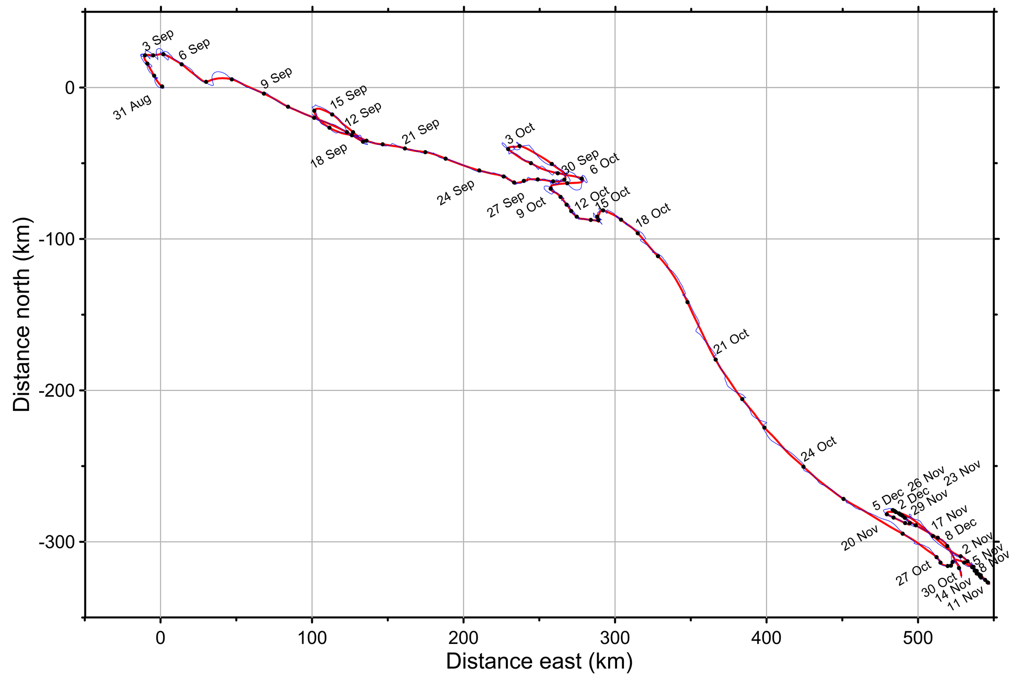
Figure 6 Progressive vector of ice drift in the Penny Strait from late August until mid-December 2009. Dots on the de-tided (red) curve are at daily intervals. Ice above the mooring became fast on 9 December.

The progressive vector of ice drift over the mooring, approximating the ice-drift trajectory through the strait, is displayed in Fig. 6. The net displacement over 102.5 d of movement in 2009 was 529 km towards the southeast, roughly the same distance as that between the Penny Strait and the edge of the continental shelf in the Prince Gustaf Adolf Sea (450 km). However because the northern entrance to the Penny Strait was blocked after 14 December, much of the ice subsequently drifting over the mooring was recently formed new and young types. The 1669 km total length of the survey track was appreciably greater than the net displacement because it continues to increase during reversals in direction driven by tide and wind. Sub-tidal events in ice movement were an alternating sequence of excursions to the northwest and southeast. Drift to the northwest was generally brief and correlated with southeasterly wind (as measured at Resolute Bay): 30 August to 3 September, 13–16 September, 30 September to 3 October and 6–8 October. Drift to the southeast occurred during the intervening periods, except that ice was almost motionless during 5–15 November. Most of the net southeast displacement occurred with prevailing northwesterly wind during 5–28 September (251 km) and 15–27 October (374 km).

3.3 Draft and underside topography of sea ice

The draft of sea ice was derived from IPS measurements of water pressure and echo time (Melling et al., 1995). Each draft value was assigned a position along the progressive vector of ice displacement calculated by integration of ice velocity. Because the IPS's field of view is about 0.8 m, redundant data were eliminated by re-sampling the ice draft at 1 m increments along the drift vector. The resulting quasi-spatial transect of under-ice topography, 1.669 million points across 1669 km of pack ice, is the starting point for scientific interpretation in this study.

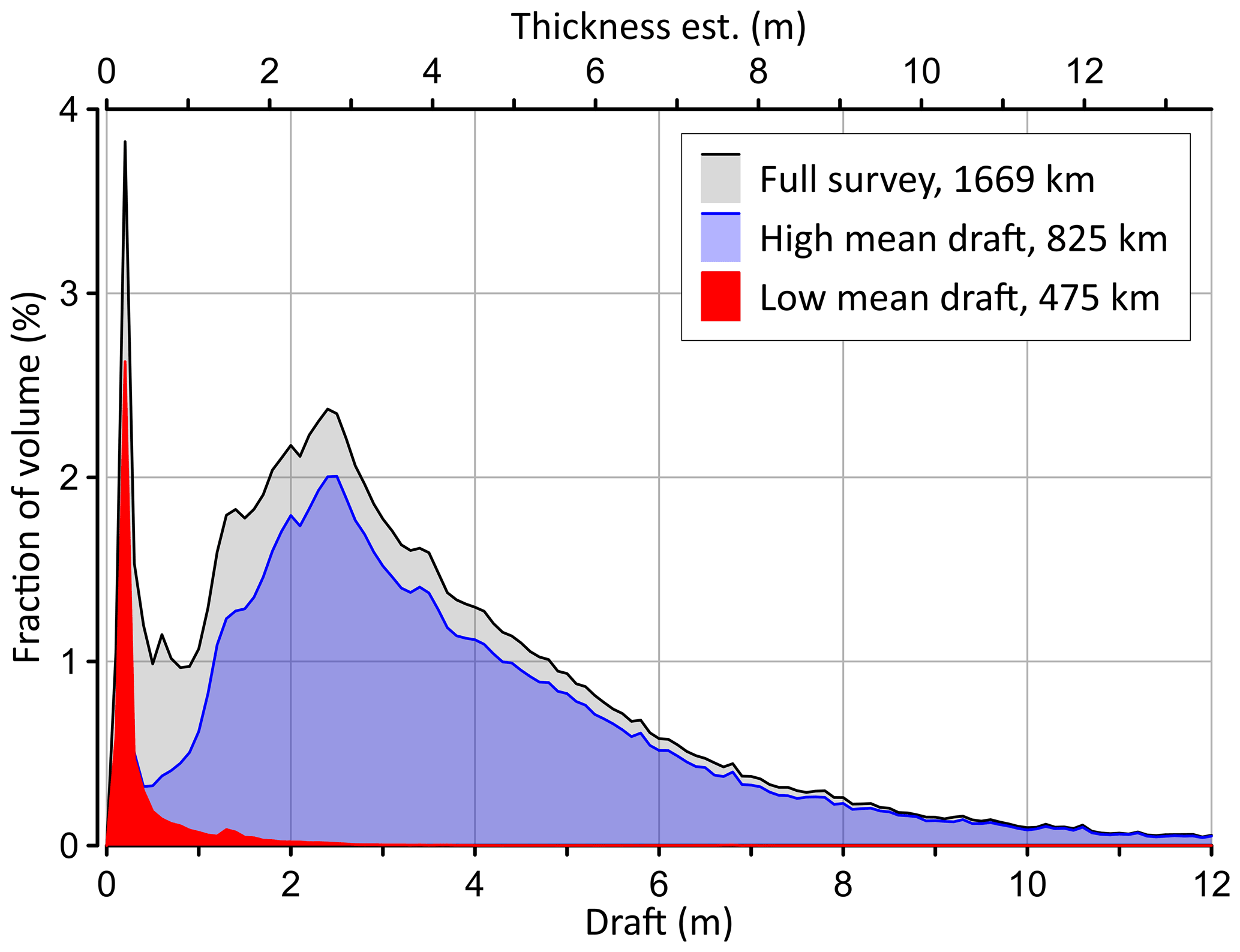
Figure 7 Fraction of ice volume versus draft. The curves represent all data, data from 33 segments of 25 km with mean draft over 2.5 m and data from 19 with mean draft under 1.5 m. Thickness on the top axis is estimated as 1.13 × draft.

Figure 7 shows the contributions to the total volume of the ice (thickness × distance × 1 m) made by ice of each draft, in 10 cm increments. The black curve displays the ice-volume distribution for the entire track; there are peaks at drafts of 0.2 and 2.45 m (old ice), separated by a minimum at 0.75 m. The red and blue curves display data from those 25 km segments with mean draft below 1.5 m and those above 2.5 m, respectively. The former peaks at 0.2 m and reveals virtually no deformed ice; this is clearly the new-ice mode. The latter peaks at 2.45 m and displays a slow roll-off to drafts characteristic of deformed ice; this is clearly the old-ice mode. The 0.75 m draft at the minimum has therefore been chosen to distinguish these two ice types in latter analysis.

Statistics of ice draft for each 25 km segment of the drift path are displayed in Fig. 8. Although sonar measures draft and not thickness, axes showing thickness have been added. A 1.13 ratio of thickness to draft has been used for the minimum and mean values, based on the reasonable assumption of near-isostatic balance at scales of 100 m and more (Melling et al., 1993). This ratio corresponds to densities of 1025 kg m⁻³ for seawater, 910 kg m⁻³ for submerged ice and 870 kg m⁻³ for sub-aerial ice without loading by snow (Timco and Frederking, 1996).

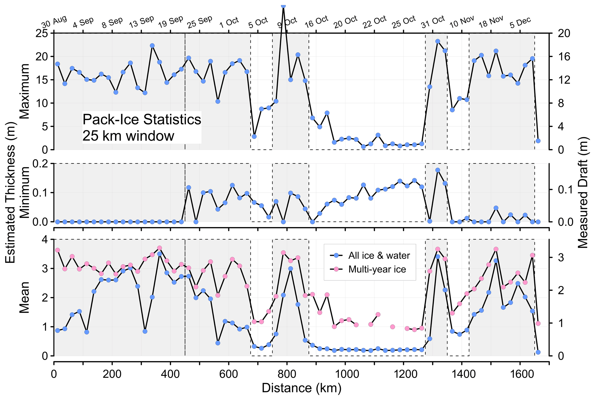
Figure 8 Statistical measures of ice draft for each 25 km segment of the drift path. The curve labelled “multi-year ice” represents the mean for ice with draft over 0.75 m. Axes on the right indicate draft and those on the left estimated thickness; conversion factors of 1.13 have been used for the mean and minimum drafts and 1.2 for the maximum, as discussed in the text. Dates of measurement are indicated on the top frame. Shading denotes intervals with appreciable multi-year ice.

Because ridges and keels are not locally in isostatic balance, the ratio of thickness to draft is variable on small (3–30 m) scales in deformed ice (Hibler et al., 1972; Melling et al., 1993). Nonetheless the ratio of maximum draft to maximum height is commonly used as a measure of the thickness of ice ridges, even though the ridge crest may not exactly coincide with the keel. In first-year ice, the ratio is quite high; Kovacs (1972) and Sisodiya and Vaudrey (1981) report 4.5 and 5.5, respectively. The ratio is lower for multi-year ice where thermal weathering and consequent consolidation affect keel draft more than sail height (Amundrud et al., 2006). Reported ratios of maximum draft to maximum height for multi-year-ice features are 3.1–3.3 (Cox, 1972; Kovacs et al., 1973; Kovacs et al., 1975), although some old ridges have yielded values as large as 5.6 (Dickens and Wetzel, 1981). The equivalent ratio of thickness to draft is about 1.3. The 12–16 m maximum drafts typical of multi-year-ice features seen in 2009 (Fig. 8) could be indicative of ice as thick as 16–21 m. However, a conservative 1.2 ratio has been used for the left-hand axis on the top frame of that figure. A keel deeper than 25 m was measured on 8 October.

The curve labelled “multi-year ice” in the bottom frame displays 25 km mean values for ice with draft exceeding 0.75 m. The overall mean of these values was 2.66 m (3.0 m thickness). Those 25 km segments for which the mean and multi-year-ice thicknesses are close in value, marked by shading in Fig. 8, will have been dominated by multi-year ice. The minimum, mean and maximum values of draft in combination reveal open water between old-ice floes until kilometre 450; open water was subsequently replaced by young ice. New ice without old floes was dominant from kilometres 875 to 1275.

4 Discussion

4.1 Evidence for change in multi-year ice of the Canadian High Arctic

As mentioned earlier, the only prior sea-ice-thickness surveys in this area were conducted in association with seismic surveys in the 1970s (Melling, 2002). The seismic work was conducted in the late winter (mid-March to mid-May) when the ice was thick enough to support the heavy sled trains used to move personnel, accommodation and equipment around this remote area. Whereas there is value in comparing the 1970s data to the present observations acquired during autumn, a comparison is informative only after adjustments that reflect the seasonal cycle of ice growth and melt. Such adjustment are obviously problematic in the absence of contemporary on-site environmental data to optimize calculations.

This paper follows the pragmatic lead of Rothrock et al. (1999) in their landmark paper on thinning Arctic pack ice. These authors adjusted ice-thickness observations from both earlier and later dates to mid-September, using values calculated by an ice-thickness model driven by 40 years of wind and temperature (but not snow depth) averaged across the Canada Basin. In our work, only the adjustment for ice thickening from autumn to late winter was necessary, a prospect more tractable than the converse because thickening by freezing is better understood than thinning by melting. Moreover, it is reasonable to assume negligible ice thickening via ridging in the area north of the Penny Strait because islands constrain the build-up of wind stress on downwind ice and inhibit the ice movement needed to build ridges during most of the winter.

Ice growth by freezing is driven by the temperature difference between the snow or ice surface and the ocean and limited by the rate at which heat can be conducted through the ice and snow, slowing as the ice and snow thicken. The calculation of the wintertime ice-growth adjustment for the 2009 data has been based on climatological values for coastal air temperature (1981–2010 epoch) (Monthly Data Report for 1980 – Climate, Environment and Climate Change Canada (https://climate.weather.gc.ca/climate_normals/results_1981_2010_e.html?stnID=1776&autofwd=1, last access: 29 July 2022)) and for snow depth on local sea ice (same epoch, https://www.canada.ca/en/environment-climate-change/services/ice-forecasts-observations/latest-conditions/archive-overview/thickness-data.html (last access: 29 July 2022)). Data from the two stations with suitable observations that are closest to the 2009 observing site, namely Resolute Bay and Eureka (locations plotted in Fig. 2), were averaged and used to drive a steady-state thermodynamic ice-growth model. Assumed values of thermal conductivity were 2.03 W m⁻¹ K⁻¹ for sea ice (Trodahl et al., 2001) and 0.31 W m⁻¹ K⁻¹ for snow (Sturm, 2002). Results based on average climatic conditions are shown in Fig. 9, comparing ice that was 0, 2 and 4 m thick on freeze-up dates of 1 October and 1 November. First-year ice starting at 0 m grows to 2.11 m by mid-May, whereas 2 m ice adds only 0.98 and 4 m ice only 0.70 m. The effects of a month's delay in freeze-up are a 3.1 % increase in thickness for first-year ice and decreases of 2.5 % and 1.0 % for 2 and 4 m ice, respectively. The increase for first-year ice reveals that the lost accumulation of snow during October more than compensates for a shorter freezing season. The sonar's first detection of new ice in the Penny Strait in late September 2009 makes 1 October the appropriate starting date for calculations.

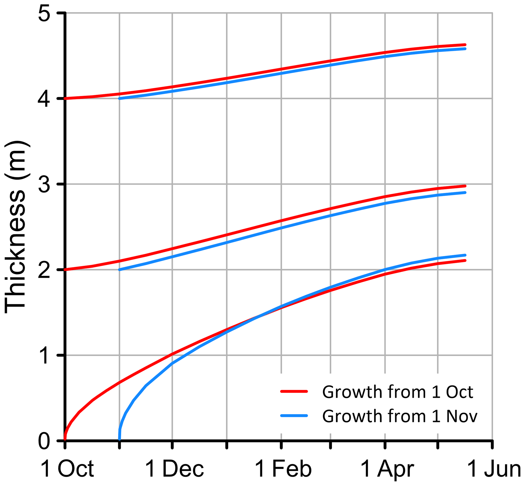
Figure 9 Calculated wintertime growth of sea ice of three initial thicknesses. The air temperature and snow depth on ice that control the growth were averages of 1981–2010 climatological conditions at Resolute Bay and Eureka.

One-standard-deviation departures from average climatic conditions were calculated from accumulated freezing degree days and snow depth on 16 May and then apportioned uniformly throughout the period of freezing.

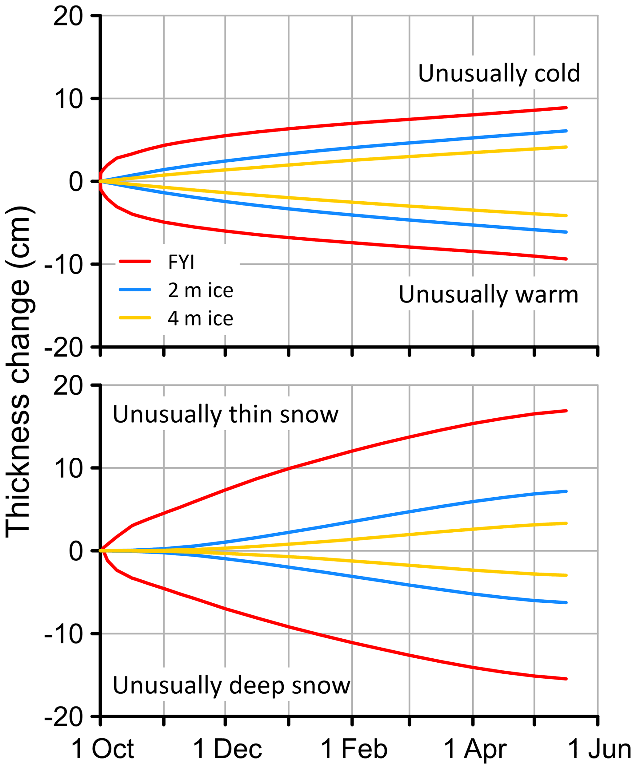
Figure 10 Sensitivity of the calculated ice-growth adjustment to ±1 standard deviation departure from average climatic conditions for air temperature and snow depth.

Sensitivity of the seasonal adjustment to these 1σ anomalies were calculated (Fig. 10). For first-year ice, the impact (8.0 %) of anomalously thin snow is almost twice that (4.3 %) of an anomalously cold winter. For 2 m ice, snow-depth anomalies are only slightly more influential than temperature anomalies (2.2 % vs. 2.0 %), whereas for 4 m ice temperature anomalies have a slightly greater influence (0.9 % vs. 0.7 %).

Ice-draft histograms measured in autumn were adjusted to late winter by shifting the bin boundaries to higher values according to the adjustments calculated for each thickness. Estimates of the late winter average thickness for each 25 km segment were then computed by summing the histogram-weighted contributions from each of the adjusted thickness bins.

Figure 11 shows estimates of the average thickness reached by the ice in each 25 km segment by the end of the 2009–2010 winter. Averages are shown for the entire ice field and for those parts of the ice field deemed to be multi-year ice by virtue of thickness – more than 0.75 m in the autumn equivalent, after adjustment, to more than 2.3 m in the spring. This figure can be compared with Fig. 8 showing the observations of the ice field in the preceding autumn. The average thickness that the observed ice field might have attained by the spring of 2010 is 2.86 m (draft 2.53 m), with a standard deviation among 25 km samples of 0.7 m. The thickness of the fraction deemed old ice in the autumn (draft more than 0.75 m) could have reached a thickness of 3.77 m (draft 3.34 m) by spring.

Multi-year ice dominated only 40 % of the 25 km segments measured in the Penny Strait in 2009. Even in present times this value, which is a result of faster ice drift through the strait, is only half the median value (70 %–80 %) in the area for which we have comparative ice-thickness data from the 1970s (Canadian 30-year ice atlas 1981–2010, https://iceweb1.cis.ec.gc.ca/30Atlas/page1.xhtml?grp=Guest&lang=en, last access: 29 July 2022). Using only the sixteen 25 km segments of the modern data with 80 % or more multi-year ice, similar to that for the 1970s observations, the mean late-winter-adjusted ice thickness is 3.75 m (sample standard deviation 0.3 m), which is very close to the alternate estimate provided above.

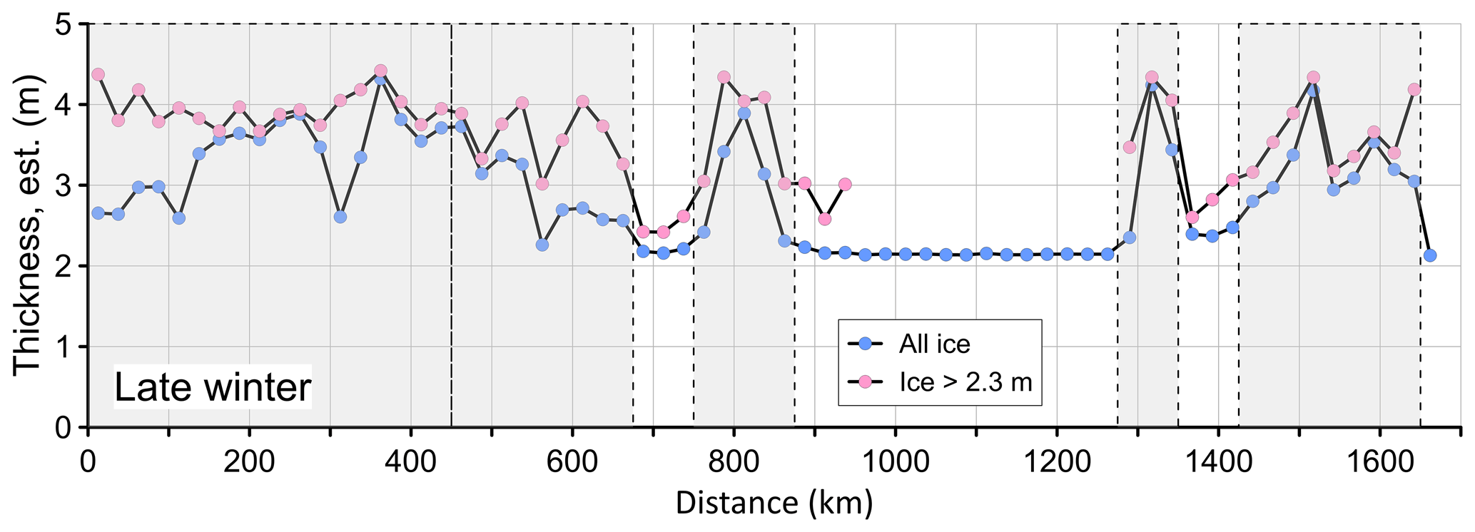
Figure 11 Average ice thickness for 25 km segments of the track line at the end of the 2009–2010 winter, estimated by forcing ice growth with monthly climatological data for air temperature and snow depth, with the assumption that no new leads or ridges formed during the winter. Shading denotes intervals with appreciable multi-year ice.

Figure 12 compares track-mean values of thickness from systematic drilling in areas “NW” and “WNW” northwest of the Penny Strait (Fig. 2) during winters in the 1970s (Melling, 2002) to the range of values estimated for multi-year ice at the same time of year in 2010, based on the 2009 measurements by sonar. For the modern data, multi-year ice was taken to be that with draft greater than 0.75 m in autumn, increasing to 2.3 m in May. The shaded band (1970s) and error bar (2009) represent sample standard deviations; the small vertical bar spans the consequence of ±1 standard deviation in air temperature and snow depth for ice that was 2 m in October; the “+” shows the effect on 2 m ice of a 1-month delay in freeze-up. The perhaps surprising result is that the estimated average thickness of multi-year sea ice up-drift of the Penny Strait in 2010 was essentially the same as it was 4 decades earlier in the 1970s.

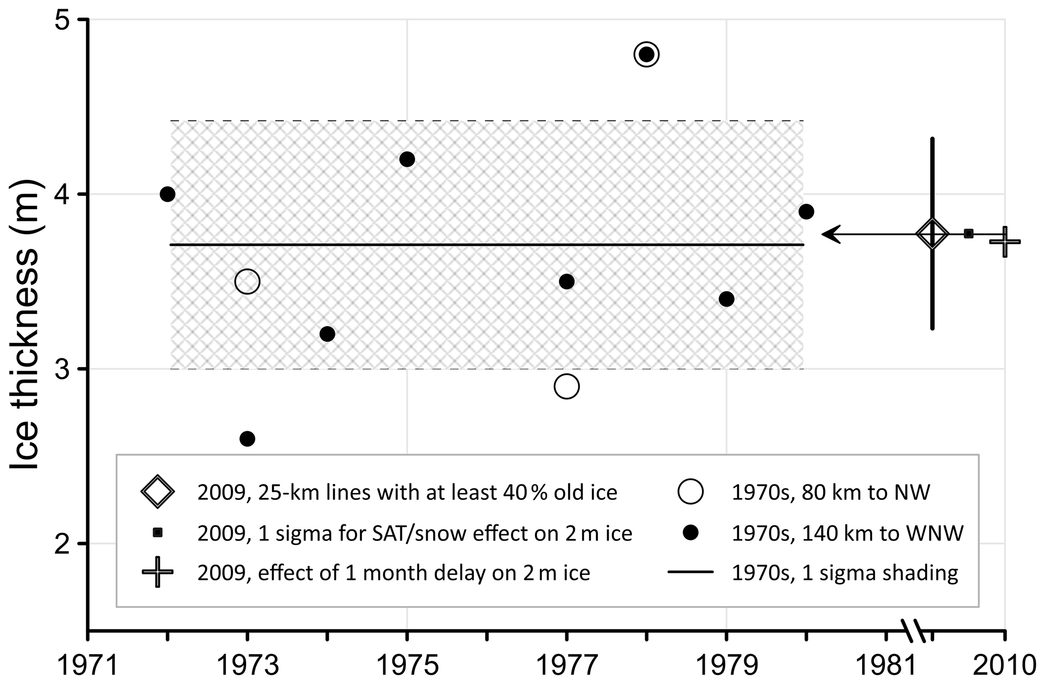
Figure 12 Track-mean ice thickness of multi-year ice from drill-hole surveys northwest of the Penny Strait during late winter in the 1970s, compared with 2010 winter values derived from observations in the autumn of 2009, as explained in the text.

Figure 13 compares the distribution of ice volume with ice thickness from the 1970s borehole data and from the 2009 measurements by sonar, adjusted to late winter values. The distributions derived from boreholes are “noisier” than the one derived from sonar because the numbers of data are so much smaller. Nonetheless it is clear that modal values were near 3 m thickness both in the 1970s and in 2009, and the roll-offs of the distributions with increasing thickness are much the same presently as they were in the past. Again the evidence suggests minimal change in the thickness of multi-year-ice population here during the last 4 decades.

Whereas a 1669 km survey in a single year does not provide the final word on change in multi-year ice on the Canadian polar shelf, the lack of change in 2009–2010 relative to the 1970s is remarkable. During this time the extent of perennial ice in the central Arctic Ocean halved (Perovich et al., 2014) and the average thickness of the mix of ice types there decreased by an estimated 1.7 m (Kwok and Untersteiner, 2011).

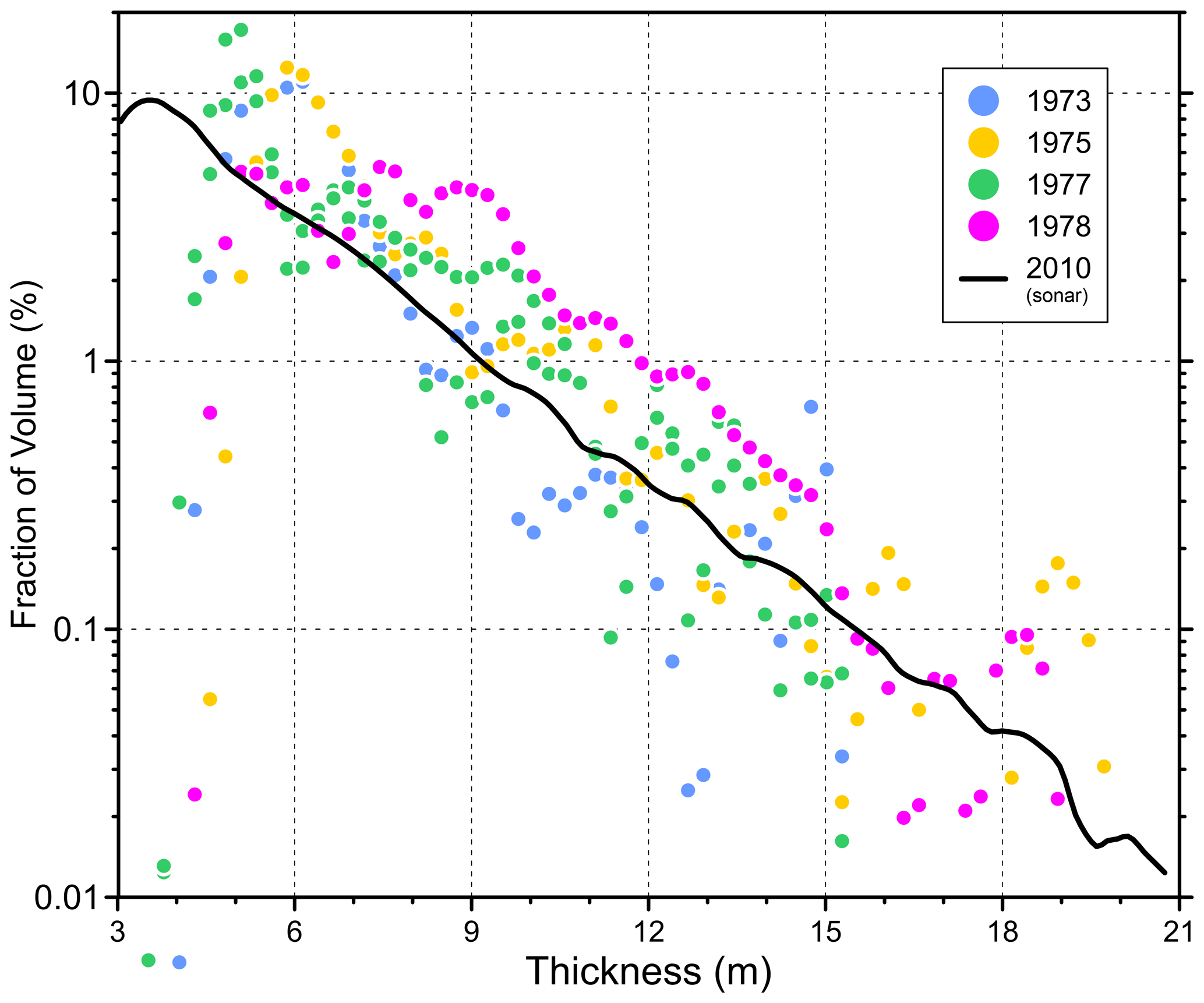
Figure 13 Distribution of pack-ice volume over ice thickness in the Penny Strait comparing recent data with surveys during the 1970s. The 2009 data have been adjusted to late winter 2010, as explained in the text.

Discussion of Arctic perennial ice in recent years has been focused more on loss factors (ice export from the Arctic Ocean, duration of residence there, duration of the thaw season, albedo feedback, cloud effects, etc.) than on formative aspects. Yet the sea-ice presence within the Arctic actually represents the difference between competing processes of ice formation and loss. The classic perspective on multi-year-ice formation is thermodynamic and traceable to the one-dimensional heat-budget model of Maykut and Untersteiner (1971).

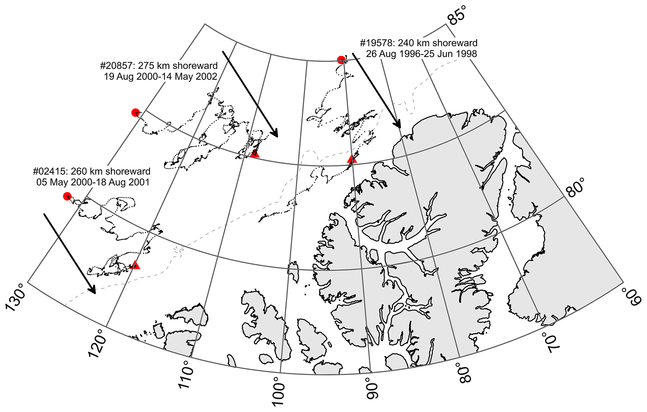
Figure 14 Tracks of three beacons on ice northwest of the Canadian Arctic Archipelago, illustrating the combined shearing and compressive deformations that allow the ice slowly to approach the coast. The starting and ending points are marked by red dots and triangles, respectively. Data courtesy of the International Arctic Buoy Programme (http://iabp.apl.washington.edu/index.html, last access: 2 August 2022).

Using this tool, it can be shown that first-year ice in the colder parts of the marine Arctic can survive its first melt season and gradually evolve into multi-year ice if the cold-season accretion of ice via latent heat loss through the top surface exceeds the warm-season ablation caused by absorption of radiative and oceanic heat. Because the latent heat lost from the top of the ice must diffuse through it from the bottom, its flux is inversely proportional to ice thickness, whereas heat gains during the thaw season are proportional to surface area and not thickness. As the ice grows thicker, the amount of new-ice accretion during winter decreases; a quasi-equilibrium maximum thickness is reached when winter's gains match the summer's losses. This maximum is about 3 m for an average seasonal cycle of climatic forcing in the High Arctic (Maykut and Untersteiner, 1971; Flato and Brown, 1996). Calculations show that increasing the maximum above 3 m by varying climatic forcing within observed limits is difficult but that increases in snow depth and ocean heat flux can readily decrease it.

Paradoxically a large fraction of the perennial ice mapped for the 1970s by Bourke and Garrett (1987) was appreciably thicker than the 3 m thermodynamic limit. Even then it was obvious that this much thicker ice must have formed by a different process. Narrow zones of much thicker ice (ridges) formed via the piling of fractured level ice are ubiquitous in pack ice (Wadhams and Horne, 1980). Indeed ridged ice 10 or more times thicker than the fragments that comprise it forms within a few hours during wind storms (Amundrud et al., 2004). Because subsequent thermal deterioration of such thick ice amounts to a few metres per year, remnants of a 30 m ridge may persist for a decade or more (Amundrud et al., 2006). However because ridge remnants are separated and relatively narrow (15–50 m), they cannot form the extensive areas of multi-year ice above 3 m thickness mapped by submarine.

However, the stamukhi zone forming the interface between fast and mobile ice is a plausible source for the large floes of thick multi-year ice, past and present. Here cyclic offshore–onshore and shearing movements of the pack driven by storms facilitate the creation of young ice in flaw leads and its subsequent compression into broad expanses of very thick ice rubble near the grounding line (see Kovacs and Mellor, 1974). The patterns of wind and ice circulation generate the highest ice pressure and rubble-forming potential along the North American side of the Arctic margin (Thorndike and Colony, 1982; Colony and Thorndike, 1984), particularly against the 2100 km stretch of coastline from northeast Greenland to the southwest limit of the Queen Elizabeth Islands. This inexorable compression against the coast is evident (Fig. 14) in the drift pattern of ice revealed by satellite tracking (https://iabp.apl.washington.edu/index.html, last access: 2 August 2022), which displays large alongshore movements in both directions that amount to relatively little net displacement alongshore, interspersed with smaller perpendicular movements that are shoreward on average.

During the 12- to 18-month duration of each track, ice drifted shoreward at about 450 m d⁻¹ – actual values were, from northeast to southwest, 360, 435 and 555 m d⁻¹. Since floes are very closely packed in this area, the shoreward movement is possible only if intervening ice is removed from the sea surface, likely via ridge building in response to compressive and possibly shearing forces at the fast-ice edge (or coastline). If the “lost” ice were 2 m thick, each day's movement would be sufficient to build along the coast a ridge of 20 m draft, 30^∘ side slope and 25 % void fraction. In the course of a year, such “daily” ridges, packed together, would form an alongshore stamukhi zone almost 30 km wide and with an average of 11 m in thickness. With time, the cold climate of this region, its highly compacted ice cover and sluggish drift towards milder climes almost guarantee the transformation of broad bands of stamukhi into thick floes of multi-year ice.

The formation and consolidation of stamukhi into broad multi-year hummock fields are storm driven, rapid and insensitive to the direct effects of atmospheric warming. Because the rate of ablation under present conditions is far too slow to eliminate the resulting thick floes in one thaw season, it is plausible that such ice persists in areas close to the formations zones with properties similar to those of past decades. Subject to uncertainty in our seasonal adjustment of observations and to currently missing knowledge of possible secular change in the mechanics of ridge building (wind stress, properties of ice and snow), we suggest that thick-ice genesis as stamukhi explains, despite changing climate, the similarity between our 2009 ice-thickness data and those from the 1970s in the Canadian High Arctic.

4.2 Hazardous ice

High average draft (correlated with high thickness and strength), wide extent and the absence of thin (viz. weak) zones are all attributes of interest in the context of ice hazards to navigation. This data set has been analyzed to yield geometric data (draft, extent) on large hazardous features within multi-year ice of the High Arctic. The focus was on floes wider than 500 m (big, vast and giant in standard nomenclature – CIS, 2005) which might be detectable using the 250 m resolution of the satellite-borne sensors commonly used for ice reconnaissance. These multi-year floes defy simple characterization (e.g. Johnston and Timco, 2008) because they are commonly freeze-bonded conglomerations of smaller floes of varying provenance, age and thickness; moreover, thaw holes produced beneath melt ponds in summer may even confound a reliable identification of floe boundaries in topographic sections. To facilitate both the delineation of floes and comparisons with borehole surveys, we have worked with a 250 m running average of the sonar-derived draft profile. Figure 15 illustrates how averaging alters the probability density of ice draft: the likelihood of both thin and thick ice decreases as the averaging scale increases while the likelihood of near-average ice increases; the multi-year-ice mode becomes more prominent and shifts to higher draft because the ice-draft histogram is positively skewed. These differences are also important to bear in mind when interpreting data from low-resolution sensors carried by aircraft and satellites.

Figure 15 Impact of along-track averaging on the probability density of ice draft.

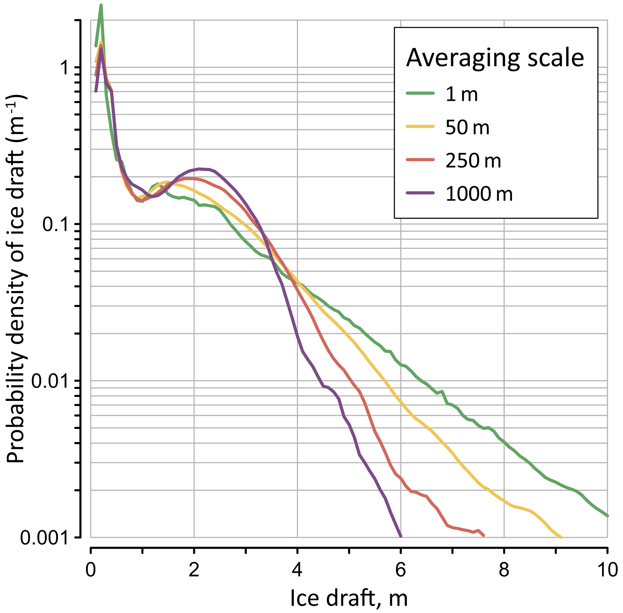
Figure 16 A 25 km segment of the section measured by sonar, The curve displays 250 m averaged values of ice draft. The red dots mark keels identified using the Rayleigh criterion. The down and up arrows mark the arriving and departing edges of floes, respectively.

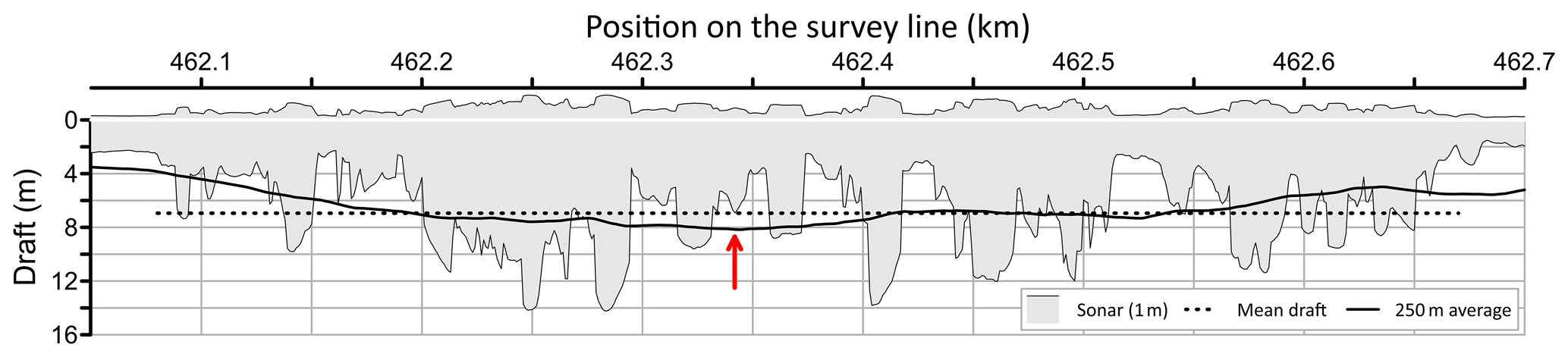
Figure 17 A 650 m section of a floe with 6.95 m average draft showing the difference between conventional ridge keels of 25 m scale in the original sonar record and the identified keel (arrow) in the 250 m averaged draft. Plotted freeboard is simply a notional scaled version of the floe's draft.

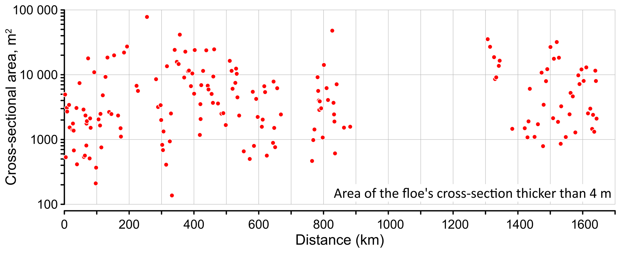
Figure 18 An index of the navigational hazard posed by individual thick floes identified along the survey path. The index in the cross-sectional area of all ice thicker than 4 m in each floe.

The Rayleigh criterion was applied to this smoothed ice-bottom relief to detect expanses of ice that were unusually thick on a 250 m scale; the reference level for draft, −2 m, enabled identification of the thickest parts of thick floes; peaks in draft were counted as separate features if intervening values dropped towards this reference level by more than half the peak value. This is an unorthodox use of the Rayleigh criterion, otherwise long established as a tool for identifying ridge keels in well-resolved ice-bottom topography (e.g. Wadhams and Horne, 1980). The boundaries of floes containing these features were taken to be those locations where the 250 m averaged draft crossed 1.5 m depth. The length of the measured chord on each floe was taken to be the length of the survey path between these crossovers; the mean draft of each floe was the average of all draft values in the measured (not smoothed) data between these points.

Figure 16 displays a segment of the smoothed ice-bottom relief, the “keels” identified within that segment and the edges of the floes in which they were embedded. These so-called keels are actually broad expanses of thicker ice, and despite their similarity in a vertically exaggerated view, they are not associated with individual pressure ridges (see Fig. 17).

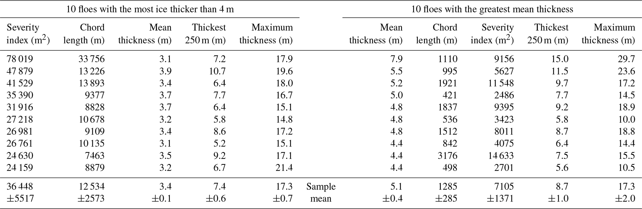
Figure 18 displays the distribution along the survey path of floes potentially hazardous to navigation. The hazard is represented by an index of severity equal to the total cross-sectional area of all ice within the feature that was thicker than 4 m; the 4 m threshold was chosen arbitrarily to be appreciably higher than the 9 ft at 3 kn (2.75 m at 1.54 m s⁻¹) capacity for continuous icebreaking by the most capable ship in service, Russia's Class-9-rated Artika. Although thick ice and large floes both present hazard, the index does not distinguish between short transects of very thick ice and long transects of thinner ice. Table 3 compares the 10 floes with the highest severity and the 10 thickest floes. The two groups of floes differ by an order of magnitude in chord length (high-index floes being larger) and by 50 % in mean thickness (high-index floes being thinner) but do not differ significantly in 1 and 250 m scale maximum thickness. The scatterplots in Fig. 19 showing all 177 floes suggest that the maximum 250 m averaged thickness of each floe had a weak tendency to increase with the size of the floe and a strong tendency to increase with its mean thickness. Within the full sample of 177 floes (plot not shown), the mean thickness of floes did not vary systematically with floe size.

Table 3 Characteristics of hazardous multi-year-ice features.

The data herein provide an opportunity to estimate how frequently floes such as those carefully measured by Johnston (2011, 2019) were likely to be encountered in the Canadian High Arctic in the late 2000s. Autonomous sonar is impartial in measuring all floes that pass overhead, whereas borehole surveys are selective. Johnston sought suitable floes during reconnaissance flights by helicopter and selected the most rugged for systematic measurement via drilling. She worked in the same area of the High Arctic during an overlapping period of time (August 2007 to April 2011). The mean of the floe-averaged thicknesses from 22 floes, each typically 20–30 holes at 10 m spacing (a 200–300 m span), was 7.60 m; the quartiles were 4.95, 7.60 and 9.38 m.

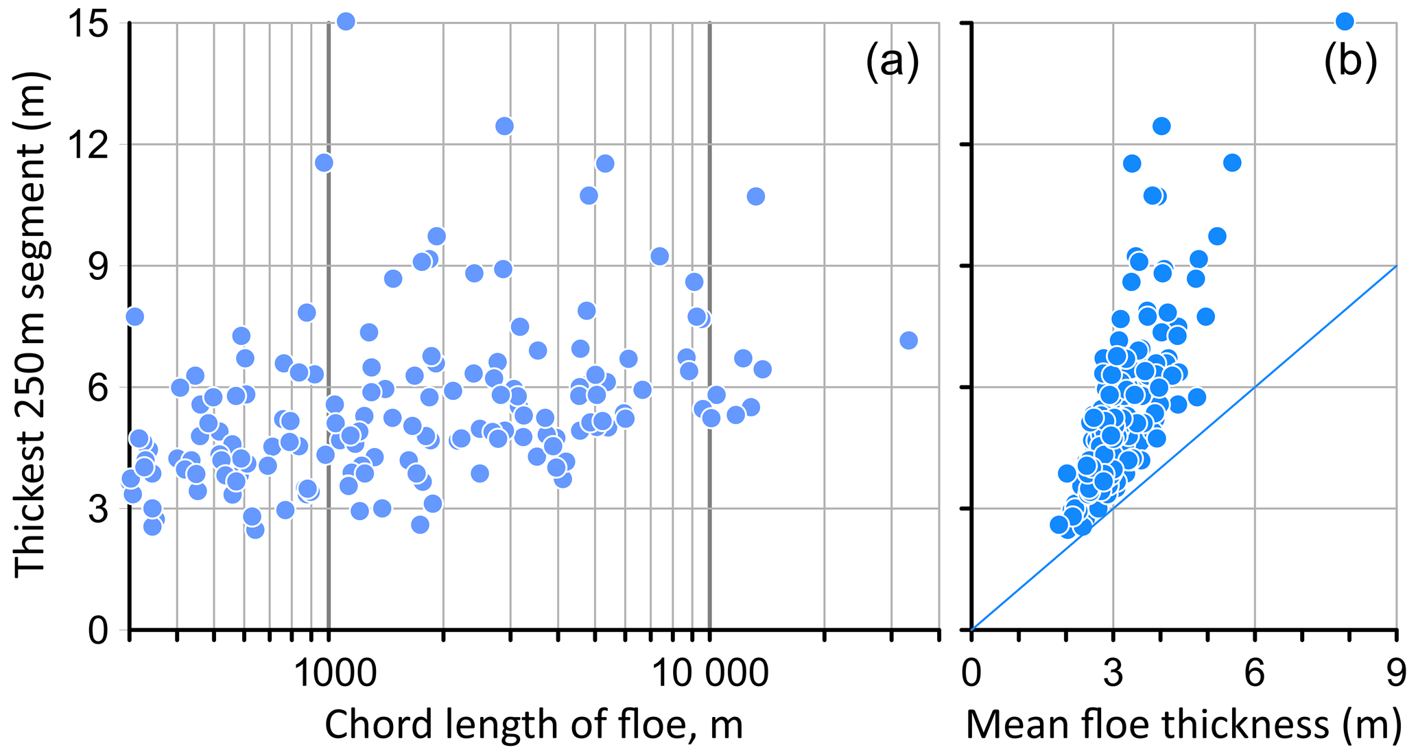
Figure 19 Scatterplot of the maximum 250 m averaged thickness of each floe against the measured chord length of that floe (a) and against the mean thickness of the floe (b).

The sonar in the Penny Strait measured ice draft across 1669.0 km of pack ice, a mix of thick old ice, thin new ice and open water. There was 738.7 km of ice within the section that had draft greater than 0.95 m. Within this thicker component of the pack, a 250 m expanse of ice with draft exceeding 4.35 m was encountered on average every 5.7 km, one exceeding 6.70 m every 42 km and one exceeding 8.30 m every 113 km (these thresholds are the drafts' equivalent to quartile thicknesses of the borehole surveys). As to be expected given the drillers' specific interest in very thick ice, 250 m expanses of ice with draft exceeding 4.35 m were much less common in the sonar record (4.36 %) than in the drill-hole surveys (75 %). The same is true of ice floes greater than 8.30 m in draft (0.22 %, versus 25 %).

However, the recurrence distances for thick ice estimated from the sonar record are not inconsistent with the airborne observer's success in finding such features. An observer flying along the sonar section at 100 kn (51.4 m s⁻¹) and looking only down would cross a 250 m expanse of 9.4 m thick ice (8.3 m draft) on average every 36 min; an observer with visibility a few kilometres to each side of the flight path could find such features in less time. Search times in the range of 15–30 min are consistent with the experience of the drill team (Michelle Johnston, personal communication, 2009).

5 Conclusions

Ice-profiling sonar installed in the Penny Strait during the 2009–2010 winter have provided modern ice-thickness data from the northern Canadian polar shelf, for comparison with prior borehole surveys during the 1970s. The two data sets provide a perspective on change at the southern margin of the notional last ice area of the marine Arctic.

The ice pack in the Penny Strait in the autumn of 2009 was a mix of multi-year floes from further north and young ice formed locally. The latter occupied about 60 % of the pack ice surveyed because the densely packed south-drifting multi-year floes spread apart as they accelerated into the strait. Old-ice and new-ice populations were distinguishable because the two populations formed distinct modes in the histogram of draft. The mean draft of those 25 km segments of the pack deemed to contain old ice (draft > 0.75 m) was 2.66 m (thickness 3.00 m).

The observations in 2009 were acquired at the end of the thaw season, whereas comparative data from the 1970s were acquired late in the freezing season. To allow inter-comparison, the modern ice-draft data were converted to thickness and then seasonally adjusted using modelled estimates of wintertime (October through mid-May) ice accretion. The resulting mean estimated thickness for multi-year ice in May 2010 was 3.77 m (sample standard deviation of 0.5 m). The average thickness from 10 borehole lines measured between 1972 and 1980 within 80–140 km of the Penny Strait, to the northwest, was also 3.7 m (sample standard deviation of 0.7 m). Moreover, the 1970s and 2010 distributions of ice volume as a function of thickness were not obviously different in modal values and roll-offs with increasing thickness. Nonetheless, we note the distinction between the absence of dramatic change over time in the thickness of multi-year-ice (this paper) and the obvious reduction in its concentration, documented elsewhere. It is noted also that the present data reveal conditions in only 1 year, in one 1669 km survey. More prolonged and widespread observations are needed to substantiate these results.

The northern Canadian polar shelf continues to present serious ice hazards to navigation, although navigational risk has decreased with the decline in old-ice concentration. A total of 177 floes of interest were identified within the 739 km of ice having 250 m averaged draft everywhere greater than 0.95 m. Their danger to navigation was assessed using four metrics: chord length, maximum 250 m average thickness, maximum thickness and the cross-sectional area of ice thicker than 4 m. The 20 most dangerous floes fell into two groups based on these metrics, those with the most ice thicker than 4 m and those with the highest mean thickness. The first tended to have modest mean thickness (3.4 m group average) and a large chord length (12.5 km group average); the second had a much smaller chord length (1.3 km group average) and, obviously, high mean thickness (5.1 m group average). The former might be considered to be freeze-bonded conglomerates of smaller multi-year-ice floes, while the later are likely fragments of very strong multi-year hummock fields. The groups differed little in their maximum thicknesses on 1 and 250 m scales. Of the floes, 46 had at least one 250 m expanse with average thickness over 6 m and 14 had an expanse averaging more than 8 m. The thickest 250 m expanses tended to occur within the smaller thicker floes.

The accelerated thermal ablation of thick multi-year ice has dominated scientific attention during recent decades. The surprising lack of change in the thickness of multi-year ice near the Penny Strait after 40 years of Arctic warming indicates need for more attention to the processes by which, as well as the locales where, it is created. We argue that the formation of Arctic multi-year-ice floes thicker than about 3 m has been and continues to be driven by pack-ice deformation rather than by surface thermal energy balance. The extreme deformation of pack ice required to build large ridges occurs within a few hundred kilometres of coastlines during strong onshore wind storms. Where such winds prevail, specifically along 2100 km of coastline bordering northern Greenland and the Queen Elizabeth Islands, ridges accumulate into wide shore-parallel bands of thick ice rubble – stamukhi zones. Ice rubble piled to a thickness of tens of metres takes many years to deteriorate in the cold High Arctic climate. Meanwhile it likely evolves into the very thick old ice still found along this coast and for hundreds of kilometres down-drift in the Beaufort Sea (via the gyre), in Baffin Bay via the Canadian Arctic outflow and in the Greenland Sea via the Fram Strait. Since there is little evidence that high-wind-stress events are decreasing in intensity, duration or frequency in response to rising Arctic air temperature, the production of very thick old ice will likely continue. The implications for the future of ice-free summers and safely navigable waters in the Arctic are obvious.