the Creative Commons Attribution 4.0 License.
the Creative Commons Attribution 4.0 License.
 | 02 Aug 2022
Evaporation over a glacial lake in Antarctica
Miguel Potes
Timo Vihma
Tuomas Naakka
Pankaj Ramji Dhote
Praveen Kumar Thakur
The study provides estimates of summertime evaporation over a glacial lake located in the Schirmacher oasis, Dronning Maud Land, East Antarctica. Lake Zub (alternately named Lake Priyadarshini and referred to throughout as Lake Zub/Priyadarshini) is the second-largest lake in the oasis, and its maximum depth is 6 m. The lake is also among the warmest glacial lakes in the oasis, and it is free of ice during almost 2 summer months. The summertime evaporation over the ice-free lake was measured using the eddy covariance method and estimated on the basis of five indirect methods (bulk-aerodynamic method and four combination equations). We used meteorological and hydrological measurements collected during a field experiment carried out in 2018. The eddy covariance method was considered the most accurate, and the evaporation was estimated to be 114 mm for the period from 1 January to 7 February 2018 (38 d) on the basis of this method. The average daily evaporation was 3.0 mm d−1 in January 2018. During the experiment period, the largest changes in daily evaporation were driven by synoptic-scale atmospheric processes rather than local katabatic winds. The bulk-aerodynamic method suggests the average daily evaporation is 2.0 mm d−1, which is 32 % less than the results based on the eddy covariance method. The bulk-aerodynamic method is much better in producing the day-to-day variations in evaporation compared to the combination equations. All selected combination equations underestimated the evaporation over the lake by 40 %–72 %. The scope of the uncertainties inherent in the indirect methods does not allow us to apply them to estimate the daily evaporation over Lake Zub/Priyadarshini. We suggested a new combination equation to evaluate the summertime evaporation over the lake's surface using meteorological observations from the nearest site. The performance of the new equation is better than the performance of the indirect methods considered. With this equation, the evaporation over the period of the experiment was 124 mm, which is only 9 % larger than the result according to the eddy covariance method.
- Article
(10275 KB) - Full-text XML
- Companion paper
-
Supplement
(475 KB) - BibTeX
- EndNote


Liquid water is increasingly more present over margins of glaciers and ice sheets and over the surface of the Arctic sea ice and Antarctic ice shelf due to rise in near-surface air temperatures enhancing snowmelt and ice melt. A large part of the meltwater accumulates in a population of glacial lakes and streams, which are typical of the lowermost (melting) zone of glaciers and ice sheets where the amount of liquid water is sufficient for both the surface and the subsurface water runoff (Golubev, 1976). The area of the melting zone is evaluated from in situ data gathered during glaciological surveys or from remote sensing data. The total area of the melting zone over the Antarctic ice sheet was estimated to be over 92 500 ± 13 000 km2 based on the in situ data collected during the period of 1969–1978 (Klokov, 1979). Estimations of the area of the melting zone in Antarctica are also available from microwave remote sensors for the summers in the period of 1979/80–2005/06, and already during this period the melting zone had covered over 25 % of the entire continent during at least five summers (Picard et al., 2007).
Recently, remote sensors and geophysical surveys have yielded evidence on a large number of glacial lakes in Greenland and Antarctica (Leeson et al., 2015; Arthur et al., 2020). In 2017, remote sensing data allowed the detection of more than 65 000 glacial (supraglacial) lakes located over the East Antarctic coast during the peak melting season (Stokes et al., 2019). The total area of these supraglacial lakes was over 1300 km2, and most of them were located at low elevations. Glacial lakes are connected by ephemeral streams into a hydrological network that may develop rapidly in the melting season (Lehnherr et al., 2018; Hodgson, 2012). During 2007–2016, the mass loss from the Antarctic ice sheet tripled relative to 1997–2006 (Meredith et al., 2019), and this explains the observed changes in physiographic parameters (volume, depth, and surface area) of many of the glacial lakes located in the East Antarctic oases (Levy et al., 2018; Boronina et al., 2019). Glacial lakes are a well-known indicator for climate change (Verleyen et al., 2003; Williamson et al., 2009; Verleyen et al., 2012). The possible effects of the glacial lakes on global sea level rise are not clear because the processes and mechanisms driving meltwater production, accumulation, and transport in the glacial hydrological network are not fully understood (Bell et al., 2017, 2019).
Among other approaches, a modelling approach can help to understand how climate warming changes the amount of liquid water seasonally formed in the glacial hydrological network including the lakes and streams. The mass (or water) balance equation of a lake is among the models applied to evaluate the volume of a lake from known inflow and outflow terms (precipitation, evaporation, surface and subsurface inflow and outflow runoff, water withdrawal), measured or modelled (Chebotarev, 1975; Mustonen, 1986). In Antarctica, various processes drive the water exchange in the local lakes, and their mass (water) budget is closely linked to the heat budget (Simonov, 1971; Krass, 1986; Shevnina and Kourzeneva, 2017), and different numbers of the terms are important while estimating their volume depending on whether a lake is connected to a glacier or not. However, for the lakes located in Antarctica, the estimates of the water budget are sensitive to uncertainties inherent in the methods applied to evaluate evaporation (Shevnina et al., 2021).
Performing direct measurements of evaporation is difficult in practice, and therefore various indirect methods are used to evaluate the evaporation over the lakes. Finch and Calver (2008) categorize such methods into seven major models (approaches) needing various meteorological and hydrological measurements, and each approach has inherent strengths and weaknesses. The pan evaporation approach has good accuracy; however the maintenance of instruments is difficult to perform in remote locations, such as Antarctica. The mass (water) balance approach needs observations of lake water budget terms (precipitation, surface and subsurface inflow and outflow runoff, water extraction, etc.) and knowledge of the lake's physiography (volume and surface area) to estimate the evaporation together with the discrepancy term. The discrepancy term depends on the uncertainties inherent in the hydrological and meteorological measurements as well as in the methods applied to estimate the terms of the lake's water budget (Finch and Calver, 2008). The application of the mass balance method for lakes located in Antarctica is not possible due to the lack of the hydrological observations. In the energy budget approach, evaporation from a lake is estimated as the term required to close the energy budget when all other terms of the budget are known (similarly to the mass balance approach). It needs a large number of observations with a high frequency of the measurements for temperature, wind speed, humidity, and radiation fluxes (Finch and Calver, 2008).
In the bulk-aerodynamic approach, the evaporation is calculated on the basis of data from the land surface properties (whether a land surface type is ice, a lake, rock, or forest; surface temperature; and surface roughness) and atmospheric variables (wind speed, specific humidity, and air temperature) in the lowermost part of the atmospheric boundary layer. In addition to observational studies on evaporation and associated latent heat flux, the bulk method is the cornerstone for parameterization of the turbulent fluxes of momentum and sensible heat in numerical weather prediction and climate models (Brunke et al., 2003). For applications of the bulk-aerodynamic method for evaporation and latent heat flux in Antarctica on the basis of in situ and remote sensing observations, see Braun et al. (2001), Vihma et al. (2002), Favier et al. (2011), and Boisvert et al. (2020).
The combination equations' approach includes the elements of both energy balance and mass-transfer approaches in the estimation of evaporation. The Penman equation (Penman, 1948) is among the most famous presenting this approach, where evaporation is calculated from the simultaneous solution of diffusion equations for heat and water vapour and the energy balance equation (Finch and Calver, 2008). A more general form of the combination equation is given by the Penman–Monteith equation (Monteith, 1965), which was developed to describe evaporation from plants (evapotranspiration). There are also a number of empirical formulas that need additional information on lake surface area, radiation, daily minimum and maximum air temperatures, etc. (Hojjati et al., 2020; Zhao et al., 2013) or require only the air temperature and relative humidity to be known (Konstantinov, 1968). The disadvantage of the empirical and combination equations' approaches is that their application is limited by the features of the location where the empirical coefficients were estimated, and there are no regional values suggested for Antarctica (Finch and Hall, 2001). The combination equations are also named the Dalton-type equations in Odrova (1979). In this study, we estimated the uncertainties inherent in four equations while estimating the summertime evaporation over the lake located in the Schirmacher oasis, East Antarctica. Among other equations, we selected the empirical equations that were previously applied while estimating the evaporation over the lakes located in Antarctica (Borghini et al., 2013; Shevnina and Kourzeneva, 2017). However, the uncertainties inherent in these estimations are not yet known due to lack of direct measurements of the evaporation.
The estimates of the evaporation are also available from atmospheric reanalyses which share results of simulations carried out applying numerical weather prediction models. Also in the most recent global atmospheric reanalysis, ERA5 of the European Centre for Medium-Range Weather Forecasts (Hersbach et al., 2020), the evaporation is estimated based on short-term weather forecasts applying the bulk-aerodynamic method.
The eddy covariance (EC) method is recognized as the most accurate method in estimating evaporation. This method was introduced more than 30 years ago (Stannard and Rosenberry, 1991; Blanken et al., 2000; Aubinet et al., 2012), but it is rarely used in remote regions. The turbulence measurements require special instruments and sensors which are difficult to maintain and operate in places such as Antarctica.
This study addresses summertime evaporation over the ice-free water surface of a glacial lake evaluated by applying various methods, namely, the eddy covariance method, the bulk-aerodynamic method, and combination equations. The EC measurements are used as a reference to evaluate the uncertainties inherent in the estimates based on the bulk-aerodynamic method and the combination equations. This information is beneficial as the EC measurements over glacial lakes are rarely available and other estimates have to be used. The field experiment was carried out on the shore of the large Lake Zub (alternately named Lake Priyadarshini and referred to throughout as Lake Zub/Priyadarshini) located in the Schirmacher oasis, East Antarctica, from 1 January to 8 February 2018.
The Schirmacher oasis (70∘45′30′′ S, 11∘38′40′′ E) is located approximately 80 km from the coast of the Lazarev Sea, Queen Maud Land, East Antarctica (Fig. 1a). The oasis is the ice-free area elongated in a narrow strip around 17 km long and 3 km wide from west-north-west to east-north-east, and its total area is 21 km2 (Konovalov, 1962). The relief is hillocks with absolute heights up to 228 m a.s.l. The oasis separates the continental ice sheet from the ice shelf, and the region allows studies on deglaciation processes and continental ice sheet mass balance components including melting and liquid water runoff (Klokov, 1979; Srivastava et al., 2012).
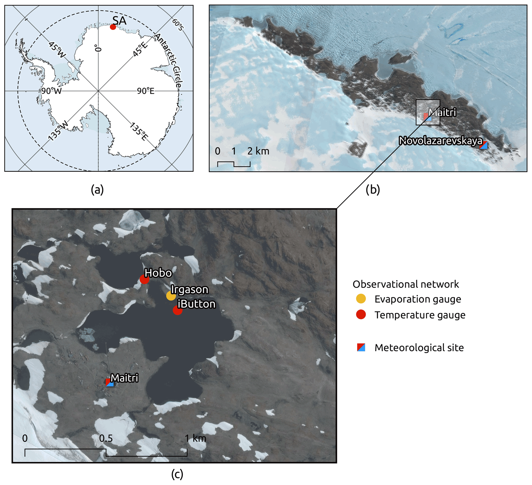
Figure 1The lakes in the study region: (a) location of the Schirmacher oasis (SA) in Antarctica; (b) the lakes of SA on the Landsat Image Mosaic of Antarctica, LIMA (https://lima.usgs.gov/, last access: 20 July 2022) given as the background; (c) the observational network in the catchment of Lake Zub/Priyadarshini with a Google Earth image given as the background, © Google Earth. The location of the meteorological sites is given according to the Antarctic station catalog (2017).
The climate of the oasis is characterized by low air humidity and temperature and persistent (katabatic) wind blowing most of the year. This easterly-south-easterly wind blows from the continental ice sheet and advects cold continental air masses to the oasis (Bormann and Fritzsche, 1995). There are two meteorological sites operating in the Schirmacher oasis (Fig. 1b): the observations were started in 1961 at the Novolazarevskaya (Novo) meteorological site (70∘46′36′′ S, 11∘49′21′′ E; 119 m a.s.l.; World Meteorological Organization (WMO) number 89512). The Maitri meteorological site (70∘46′00′′ S, 11∘43′53′′ E; 137 m a.s.l.; WMO number 89514) opened in 1989 and is located 5.5 km from the Novo site. Both meteorological sites are included in a long-term monitoring network, and their measurements are performed according to the WMO's standards (Turner and Pendlebury, 2004). The meteorological data gathered at these two stations are available from the British Antarctic Survey datasets (https://www.bas.ac.uk, last access: 14 December 2018). Table 1 shows weather conditions during the austral summer 2017/18 and averaged over the period of 1961–2010 according to the observations at the Novo site (the data given by the Arctic and Antarctic Research Institute at http://www.aari.aq/default_ru.html, last access: 7 December 2021).
Table 1The monthly minimum, mean, and maximum values for the meteorological parameters calculated for the period of 1961–2010 (the values are separated by a slash), and their monthly average calculated for the austral summer 2017/18. The values are evaluated from the observations at the Novo site.
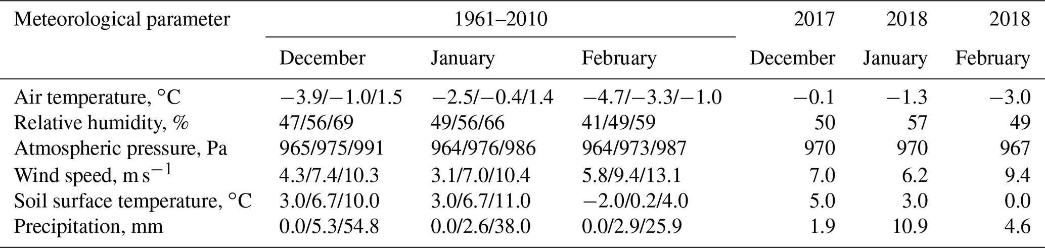
The field experiment lasted 38 d in January–February 2018. Generally, the weather during the experiment was colder and less windy than the monthly means estimated for the period 1961–2010, while the relative humidity and amount of the precipitation were close to them (Table 1). According to data from the Novo meteorological site, during the period of the campaign the daily air temperatures ranged from −8.3 to 2.8 ∘C and the wind speed from 1.5 to 14.3 m s−1, with an average of 6.2 m s−1. The observations at the Maitri site were very similar to those at the Novo site, with the Pearson correlation coefficient between the daily series of air temperature, relative humidity, and wind speed varying from 0.95 to 0.98. According to the Maitri meteorological site, the wind speed varied from 1.6 to 14.4 m s−1, with an average of 6.7 m s−1. The air temperature ranged from −8.3 to 2.1 ∘C, with an average of 1.5 ∘C. The average relative humidity during the summer was 54 %.
More than 300 lakes are mapped in the Schirmacher oasis (Fig. 1b), and many of the lakes stay free of ice in the summertime for almost 2 months (Simonov, 1971; Richter and Borman, 1995; Kaup and Haendel, 1995; Kaup, 2005; Phartiyal et al., 2011). The hydrological cycle and changes in the lakes' volume are modulated by the seasonal weather cycle (Sokratova, 2011; Asthana et al., 2019). The lakes' physiography is available from bathymetric surveys for only the largest lakes located in the Schirmacher oasis (Simonov and Fedotov, 1964; Loopman et al., 1988; Khare et al., 2008; Dhote et al., 2021). This study focuses on Lake Zub/Priyadarshini, which is among the largest and warmest waterbodies of the Schirmacher oasis. The lake's surface area is 35×103 m2; its volume is over 10×103 m3; the maximum depth is 6 m (Khare et al., 2008; Dhote et al., 2021). Lake Zub/Priyadarshini occupies a local depression and is fed by two inflow streams present in warm seasons. The outflow from the lake occurs via a single stream. The lake stays free of ice for almost 2 summer months from mid-December to mid-February (Sinha and Chatterjee, 2000). The water level (and volume) of Lake Zub/Priyadarshini has been reducing continuously, and in 2018 the lake water level lowered by approximately 0.4 m (Dhote et al., 2021). The lake is used as the water supply for the year-round Indian scientific base Maitri.
Gopinath et al. (2020) used water samples collected from 12 lakes (including Lake Zub/Priyadarshini) located in the Schirmacher oasis to recognize major sources of water in the lakes. The samples were analysed with the isotope method (Ellehoj et al., 2013), and the isotopic concentrations show that Lake Zub/Priyadarshini is mostly sourced by the melting of the adjacent glaciers. Lake Zub/Priyadarshini is the lowest in the chain of the glacial lakes sourced by the ice/snow melting in the lowermost zone of the glaciers, and we estimated that more than 60 % of its catchment area is covered by rocks. This allows for the specific thermal regime and water balance of this glacial lake, which is among the warmest in the oasis: its water temperature rises up to 8–10 ∘C in January (Ingole and Parulekar, 1990). Such water temperatures are typical of the landlocked lakes (Simonov, 1971).
Lake Zub/Priyadarshini presents ideal conditions to study evaporation over a glacial lake, and to plan the field experiment, we accounted for the location to set up the EC measuring system. Selection of the exact site for EC measurements requires, among other things, data on the prevailing winds and their fetch over the lake and naturally also accessibility for regular maintenance. To evaluate the prevailing wind direction, we used 6-hourly synoptic observations at the Novo site available from the British Antarctic Survey Dataset (https://www.bas.ac.uk, last access: 14 December 2018) covering the period 1998–2016. We calculated the number of cases when wind was blowing from 36 sectors, each 10∘ wide, and then defined the prevailing wind directions (marked with the black arrows in Fig. 2). The prevailing wind directions range from 110 to 140∘.
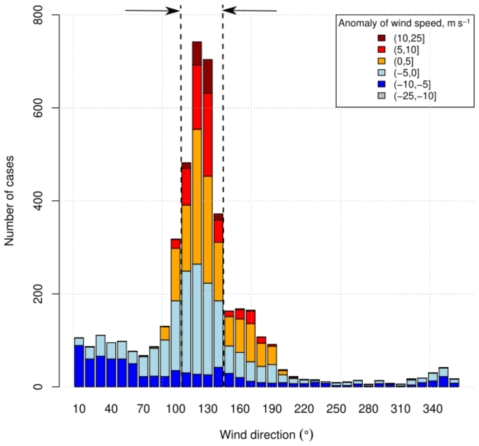
Figure 2Wind direction and wind speed anomalies for 2 austral-summer months (December and January): the arrows indicate the prevailing wind direction. The data are extracted from the British Antarctic survey dataset (available at https://www.bas.ac.uk, last access: 14 December 2018) for the period 1998–2016.
We also evaluated the wind speed anomalies of each 10∘ sector given in colour codes in Fig. 2. The anomalies were calculated as the difference between the observed value and the long-term mean value estimated for the period of 1998–2016 in our study. The positive wind speed anomalies are often observed within the range of the prevailing wind directions (marked with yellow, red, and brown in the legend of Fig. 2). Therefore, one can expect the majority of strong winds from these directions. The region of the study is featured by persistent katabatic winds blowing from the continental interior. Figure 2 shows that most of the winds come from a direction that represents the katabatic winds. However, it is not guaranteed that all these winds are entirely of katabatic origin, and some winds may be driven by a combined effect of katabatic and synoptic forcing.
3.1 Data
In the 2017/18 field experiment, we collected the hydrological and meteorological observations needed to evaluate the evaporation over the surface of Lake Zub/Priyadarshini. The observational network included two water temperature sensors (named HOBO and iButton) and the EC station (named IRGASON); we also utilized the observation at the Maitri meteorological site (Fig. 1c). The EC station has a flux tripod mast equipped with an IRGASON instrument from Campbell Scientific. The IRGASON consists of a 3D sonic anemometer and two gas analysers measuring CO2 and H2O concentrations, with a control unit for all the measurements. The IRGASON was installed on the shore of the lake to collect high-frequency data on wind speed/direction and water vapour concentration needed to evaluate evaporation with the EC method (Fig. 3a). The flux tripod was placed 5–6 m inland of the shoreline of Lake Zub/Priyadarshini for the period of 1 January to 7 February 2018 (Shevnina, 2019). The meteorological parameters (air temperature, wind speed, and relative humidity) were measured simultaneously at the Maitri meteorological site and at the IRGASON. The data gathered by the hydrological and meteorological sensors cover various observational periods (Table 2). The shortest 14 d period with the measurements is available for the iButton temperature sensor, and this period lasted from 27 January to 9 February 2018.
Table 2The hydrological and meteorological data collected during the field experiment in the summer 2017/18: “–” no information available.
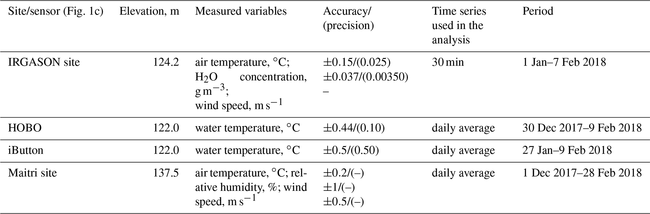
Table 2 shows the information on the accuracy and resolution of the sensors according to the technical specifications given by the manufacturers. Ramesh and Soni (2018) give the information for the sensors installed at the Maitri site. On the 30 December 2017 the elevation of the lake water level was measured by the geodetic instrument Leica CS10; the level was 122.3 m, WGS84 ellipsoid vertical datum. We used this elevation to calculate the elevation of the HOBO, iButton, and IRGASON temperature sensors. The Leica CS10 instrument was used to measure the elevation of the Maitri site in January 2018 (Dhote et al., 2021).
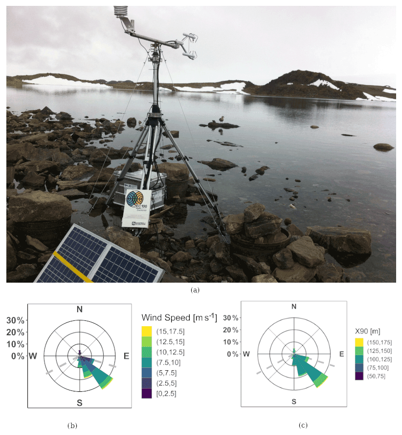
Figure 3The experiment on the coast of Lake Zub/Priyadarshini: (a) IRGASON installed on the lake shore (6 January 2018); (b) wind speed and direction measured at the IRGASON site – dashed line indicates the footprint wind sector; (c) the footprint length estimate (X90).
The footprint is an important concept for evaluating the fluxes correctly with the EC method. The footprint is defined by a sector of wind direction covering the source area, and its length depends on the sensors' height, roughness, and atmospheric stability (Kljun et al., 2004; Burba, 2013). The footprint was estimated according to the parameterization proposed by Kljun et al. (2004), and the 90 % contribution (X90, m) is shown in Fig. 3c. The footprint area depends on the location of the EC station, the height of its sensors, the roughness of the upwind surface and the stratification of the upwind atmospheric surface layer (Kljun et al., 2004; Burba, 2013). The IRGASON was settled at the height of 2 m above the ground, which yields footprint lengths of less than 200 m. In this study the footprint length was defined as X90 and represented 90 % of the cumulative contribution to the fluxes (Fig. 3c). This distance is less than twice that between the IRGASON and the shore of Lake Zub/Priyadarshini in the east-south-east direction (Fig. 1c), and it ensures that the measured data are representative only for the lake and free of contamination from the upwind shore. The tower height of 2 m generates a blind zone near the tower, so the stones on the downwind shore do not affect the fluxes.
The location of the EC tower accounted for the prevailing wind directions (Fig. 2), meaning that the footprint area is mainly represented by the lake surface. We filtered out data outside the footprint (Fig. 3b). Gaps in the wind direction were replaced with the average values of the neighbouring 30 min blocks. The IRGASON's raw data consisted of values measured at a frequency of 10 Hz. We used these raw data to calculate a 30 min time series of evaporation, turbulent fluxes of momentum, sensible heat, and latent heat, as well as air temperature, wind speed, and wind direction. The daily evaporations were calculated as a sum of the 30 min time series. The low observation height of 2 m guarantees that the vertical divergence of the water vapour flux is negligible, and therefore the water vapour flux observed at the height of 2 m represents the surface evaporation.
To allow the estimation of evaporation by the combination equations, measurements of the water temperature are needed; and we measured the lake's surface water temperature during the 38 d of the experiment period. We also measured the water temperature of the lake's surface with two sensors during the period of 14 d: the iButton temperature sensor was installed in Lake Zub/Priyadarshini at a depth of 0.2 m and was placed ahead of the EC station (IRGASON) toward the prevailing wind directions. The HOBO temperature sensor was deployed at a depth of 0.2 m in the end of the stream inletting the neighbouring lake (Fig. 1c). This stream is an outlet of Lake Zub/Priyadarshini, and we assumed that the observations collected by the HOBO were representative of the stream more than of the neighbouring lake itself. The accuracy of both temperature sensors is similar, and the resolution of the HOBO temperature sensor is better than the iButton's precision. The lake surface temperature was measured every 10 min, and we further calculated the daily average time series of the water temperature in the lake. The mean difference between the measured lake surface temperature is −0.05 ∘C, and it is comparable to the precision of the iButton temperature sensor (Table 2). The correlation coefficient between the 10 min series of the water temperature measured by the two temperature sensors, HOBO and iButton, was equal to 0.94 (Fig. 4a). We further used the measurements collected by the temperature sensor with better precision (HOBO) to estimate the evaporation over Lake Zub/Priyadarshini in January 2018.
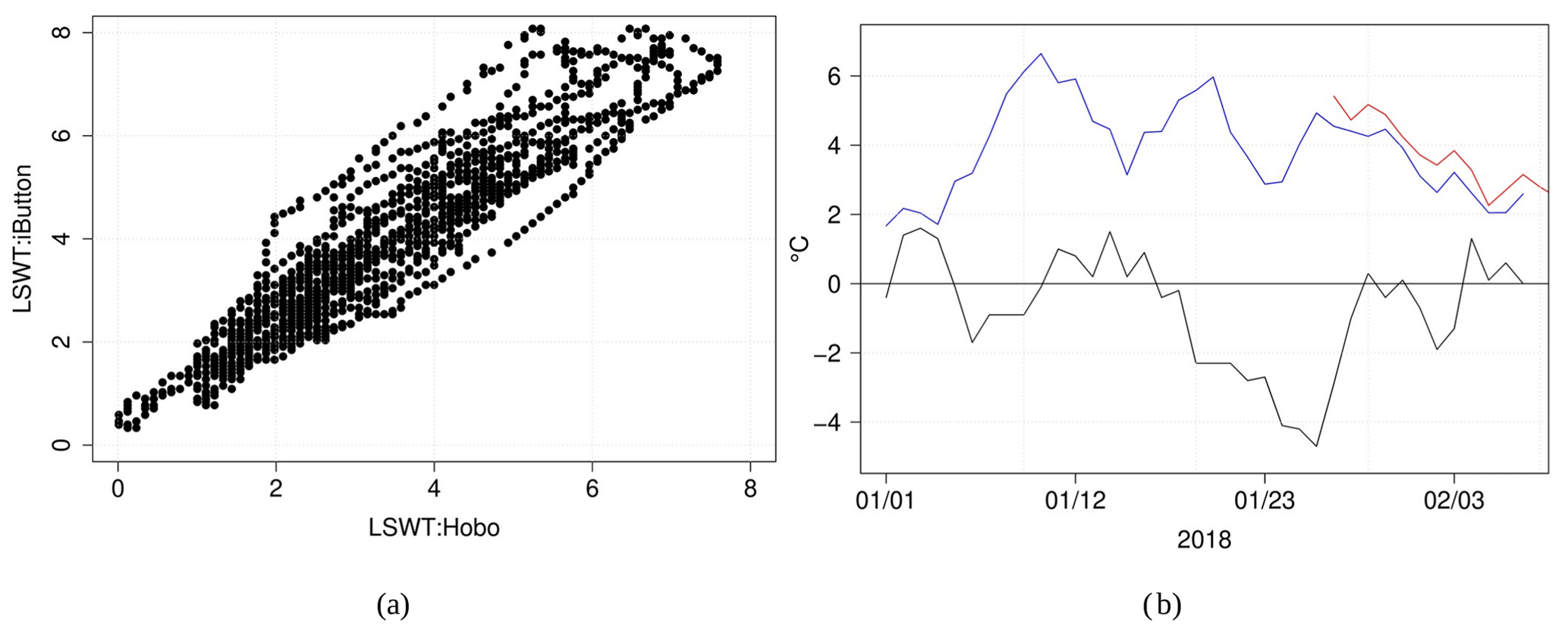
Figure 4(a) The 10 min lake surface water temperature (LSWT) measured by the HOBO temperature sensor (x axis) and iButton sensor (y axis); (b) daily time series of the lake surface water temperature measured by the HOBO (blue) and by the iButton (red) and the air temperature measured at the Maitri site (black).
Figure 4b shows the daily time series of the lake surface water temperature and air temperature during the period of the experiment on the shore of Lake Zub/Priyadarshini. Sinha and Chatterjee (2000) reported that Lake Zub/Priyadarshini was thermally homogeneous down to the bottom almost from mid-January 1996 to mid-February 1997. In this study, we assumed that Lake Zub/Priyadarshini had no thermal stratification during the austral summer season like the many other ice-free lakes located in the Antarctic oases (Sokratova, 2011).
In our calculations based on the combination equations we applied the data collected by the meteorological sensors installed at both the Maitri and the IRGASON sites at a different height above the ground. The height of the temperature sensor and gas analyser of the IRGASON is lower than the sensors at the Maitri site, and therefore we used the logarithmic approximation of the wind profile to correct the wind speed data measured at the Maitri site, for which we estimated a constant aerodynamic roughness length of 0.002 m (Stull, 2017). We did not use any height correction for the data on the relative humidity and air temperature since their changes with elevation are negligible in our case (Tomasi et al., 2004).
3.2 Methods
3.2.1 Eddy covariance method
To evaluate the evaporation with the direct EC method, we used the data collected by the IRGASON installed on the shore of Lake Zub/Priyadarshini. The IRGASON raw data were measured with a frequency of 10 Hz, which were further analysed in the following steps. In the first step, we discard data where more than 50 % of the measurements (10 Hz) present malfunctions in the 30 min block. These data are detected in two diagnostic variables, one for the sonic anemometer and the other for the gas analyser. Second, we excluded all data automatically flagged for low quality and the data with a gas signal strength less than 0.7 (or 70 % of the strength of a perfect signal). The gas signal strength is usually lower than 0.7 during rainfall, which was not observed in January 2018 in the Schirmacher oasis. Generally, rainfall is rare along the East Antarctic coast and occurs 22 d per year at most (Vignon et al., 2021). In the third step, the spikes were removed applying the method by Vickers and Mahrt (1997), fixing the threshold window of 3.5 standard deviations for horizontal wind speed and H2O and 5.0 for vertical wind speed. This procedure was repeated up to 20 times or until no more spikes were found. Finally, we obtained, among other things, the 30 min fluxes of momentum, sensible heat, and latent heat (evaporation), as well as the water vapour concentration (see the Supplement). The evaporation over the lake was calculated only by those values collected within the footprint of the ice-free surface of the lake. Therefore, we filtered the data outside the footprint which covered the wind directions within the range of 105–240∘ (Fig. 3b) to account only for those values collected within the lake surface area. Figure 5 shows the 30 min time series of the evaporation obtained and the average water vapour obtained with the IRGASON; the red dots indicate the measurements coming from outside the footprint, and it is visible that these red dots mainly represent lower evaporation values. We excluded 18 % of the total data from further consideration after the three-step filtering. To fill these gaps we replaced the excluded values by the mean value, which was estimated from the time series of 30 min values. We also evaluated the relative humidity from the water vapour concentration as given by Hoeltgebaum et al. (2020).
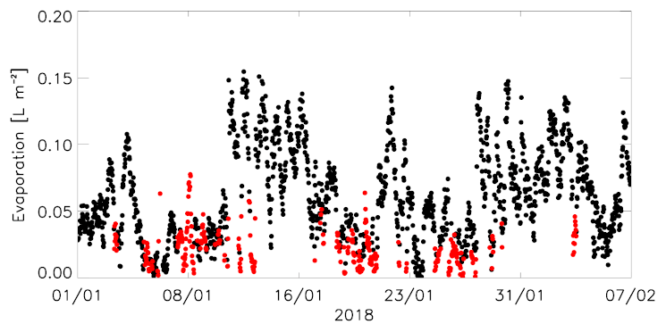
Figure 5The 30 min time series of the evaporation obtained with the EC method: the red dots indicate the measurements coming from outside the footprint.
Uncertainties in the estimation of evaporation by any method include instrumental errors associated with the specific instrument. Aubinet et al. (2012) suggest three methods that allow the quantification of the uncertainty in the EC method. In this study, we applied the paired-tower method to evaluate the uncertainties inherent in the EC method, taking advantage of an intercomparison campaign in Alqueva reservoir (Portugal) in October 2018, where our instrument was installed side by side with an equal instrument. The instrumental error does not depend on the region where the instrument is used, and therefore the intercomparison may be performed elsewhere. The relative instrumental error estimated in this intercomparison campaign was 7 % (see the Appendix). The uncertainties in the EC method also include the errors due to the filtering of measurements within the footprint area. The large number of filters and corrections that we applied to the EC data allowed us to reduce the errors and uncertainties. Even the EC method itself has some errors and uncertainties, but it is the most versatile and accurate method to measure evaporation.
3.2.2 The bulk-aerodynamic method
In the bulk-aerodynamic approach, evaporation is defined as the vertical surface flux of water vapour due to atmospheric turbulent transport. It is calculated from the difference in specific humidity of the surface (i.e. ice or water for which the specific humidity equals the saturation specific humidity that depends on the surface temperature) and the air, as well as the factors that affect the intensity of the turbulent mixing: wind speed, surface roughness, and thermal stratification (Boisvert et al., 2020; Brutsaert, 1982). The evaporation based on the bulk-aerodynamic method is calculated as follows:
where E is the evaporation (in kg m−2 s−1, which we in the following convert to mm d−1), ρ is the air density (in kg m3), is the turbulent transfer coefficient for moisture (unitless), qs is the saturation specific humidity at the water surface of the lake (kg kg−1), is the air saturation specific humidity (kg kg−1), and wz is the wind speed (m s−1). The subscript z refers to the observation height (here 2 m). The turbulent transfer coefficient for moisture depends on the atmospheric stratification: for under neutral stratification () we applied the value of 0.00107 based on previous measurements over a boreal lake (Heikinheimo et al., 1999; Venäläinen et al., 1998). This allows us to better take into account the different regime of turbulent mixing over a small lake compared to the sea (Sahlée et al., 2014).
Since the stratification of the atmosphere is not always neutral, we took into account its effects on the turbulent transfer coefficient as follows:
where is the neutral drag coefficient for the lake surface, k is the von Kármán constant (0.4), ψm and ψq are empirical stability functions, and L is the Obukhov length (in metres). The Obukhov length is
where ρ is the air density, cp is the specific heat, u∗ is the friction velocity, θz is the air potential temperature, g is the acceleration due to gravity, and H is the surface sensible heat flux. The Obukhov length (Obukhov, 1946) is the key element of the Monin–Obukhov similarity theory (Monin and Obukhov, 1954; Foken, 2006) and is needed to adjust the bulk transfer coefficients to the actual stratification in the atmospheric surface layer. In our calculations, the neutral drag coefficient equals 0.00181 as suggested by Heikinheimo et al. (1999). For ψm and ψq, we used the classic form by Businger et al. (1971) for unstable stratification and that of Holtslag and de Bruin (1988) for stable stratification. The values by Heikinheimo et al. (1999) were given for z=3 m and converted to our observation height of 2 m using Launiainen and Vihma (1990), and the same algorithm was applied to iteratively solve the interdependency of the turbulent fluxes and L. The latent heat flux is obtained by multiplying the evaporation rate by the latent heat of vaporization.
3.2.3 The empirical equations
Most of the empirical equations are based on a simple mass-transfer relation between the evaporation rate and the water deficit and wind conditions. The general form of the relation reads ), where K is an empirical function approximated with a small number of coefficients. Among others, Shuttleworth (1993) suggests two mass-transfer equations for the estimation of evaporation from the surface of lakes and ponds depending on their surface area. In this study, we used his formula for waterbodies in the range of 50 m km located in regions with a relatively arid climate. The equation reads ), where E is the evaporation in millimetres per day (mm d−1), A is the surface area in square metres (m2), w2 is the 2 m wind speed in metres per second (m s−1), and es and e2 are the surface water and air vapour saturation pressure in kilopascals (kPa). In this study, we used this formula to estimate the daily evaporation from Lake Zub/Priyadarshini, whose surface area was estimated as 350 000 m2 in 2016 (Dhote et al., 2021). The method by Shuttleworth (1993) has been used to evaluate evaporation over small lakes located in Antarctica (Borghini et al., 2013); however the scope of uncertainties inherent in the method is not known.
Penman (1948) first suggested taking the elements of the mass-transfer and energy budget approaches into the estimation of evaporation from open water, and his formula is one of the combination equations (Shuttleworth, 1993; Finch and Calver, 2008). In this study, we applied two combination equations to calculate daily evaporation: E=0.26 and E=0.26 ( adopted from Tanny et al. (2008), where these formulas are referred to Penman (1948) and Doorenbos and Pruitt (1975), respectively. These equations are among those most often used in hydrological practice (Finch and Calver, 2008), and therefore we have chosen them in this study. We also used the formula E=0.14 , which has been applied to evaluate evaporation from lakes located in northern Russia (Odrova, 1979). In these equations, es and e2 are the surface water and air vapour saturation pressure (millibars), and we calculated them according to Tetens's formula given in Stull (2017). The method by Odrova (1979) has been used in calculations of evaporation over glacial lakes located in Antarctica (Shevnina and Kourzeneva, 2017) without estimated uncertainties. We calculated daily evaporation separately using the meteorological observations collected at the Maitri site and at the lake shore (IRGASON site).
The empirical coefficients in the combination equations usually limit their applicability to the region where such coefficients are obtained (Finch and Hall, 2005). The empirical coefficients in four selected equations are evaluated from data gathered in regions with different climates, and therefore they probably will not be applicable to lakes located in Antarctica. In this study, we suggested the regional empirical coefficients based on the daily series of evaporation estimated by the direct EC method and the meteorological observations at the Maitri site, which is the nearest meteorological site to the lake. The evaporation (E, mm d−1) was evaluated with the model , where A and B are fitted with empirical coefficients and (es−e2) is expressed in millibars (mbar). The efficiency of fitting the coefficients was performed on the same data for the experiment (lasting 38 d); the least-squares method was applied in the fitting of the empirical coefficients in our relationship.
Evaporation by the indirect methods was compared to the direct (EC) method in order to find the method with the lowest scope of the uncertainties and, therefore, the method of the highest efficiency. We applied the Pearson correlation coefficient (PR), the root mean square error (RMSE , where EEC is the evaporation by the eddy covariance method and Emod is evaporation by an indirect method), and the (SSC) criteria to evaluate the scope of the uncertainties inherent in the indirect methods (Moriasi et al., 2007; Popov, 1979). The SSC reads as follows: , and . In these formulas, is the mean evaporation (mm), n is the length of the series (38), and m is the number of empirical coefficients in the relationships (equal to 2). Overall, a new method is acceptable for further use in hydrological practice if the SSC value is less than 0.8 (Popov, 1979).
4.1 Evaporation
We considered the direct EC method as the most accurate, providing the reference estimates for the evaporation over the lake surface (Finch and Hall, 2005; Tanny et al., 2008; Rodrigues et al., 2020). According to the EC method, the daily evaporation varied from 1.5 to 5.0 mm d−1 with the average being equal to 3.0 mm d−1, and the standard deviation was ±1.1 mm d−1. The average was calculated by dividing 114 mm of evaporated water (which is the sum of the 30 min series of evaporation) by the number of days in the observational period (which is 38). The sum of the evaporation over the period of the field experiment is 94 mm if we simply exclude the gaps in the 30 min series.
We estimated the uncertainties inherent in the indirect methods by comparing their results with those based on the EC method. The average daily evaporation was 2.0 mm d−1 calculated by the bulk-aerodynamic method with the mass-transfer coefficients after Heikinheimo et al. (1999), and this value is approximately 30 % less than those estimated by the EC method. It is also the best estimate among the indirect methods (bold notation in Table 3). All combination equations underestimated the evaporation over the lake surface by over 40 %–72 %, and the method by Odrova (1979) yielded the greatest underestimation of the mean daily evaporation over the lake surface. The uncertainties in the estimates by indirect methods are approximately the same for both cases of the input data (Maitri and IRGASON).
Table 3The daily evaporation (mm d−1) over the surface of Lake Zub/Priyadarshini for the period of 1 January–7 February 2018: SD is the standard deviation; r is the ratio between the sum EEC divided by the sum Emod. Bold: best estimate among the indirect methods.
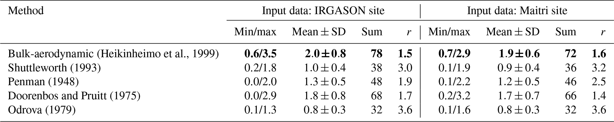
Figure 6 shows the daily evaporation estimated by the direct EC against those estimated by the four indirect methods calculated based on the meteorological observations collected at two measurement sites: Maitri and IRGASON. There was not a large difference in the results, and therefore we can recommend using the meteorological observations gathered at the Maitri site in further estimation of evaporation. Table 4 gives a summary of the scope of the uncertainties in and efficiency of the indirect methods to model the day-by-day series of the evaporation with the selected criteria.
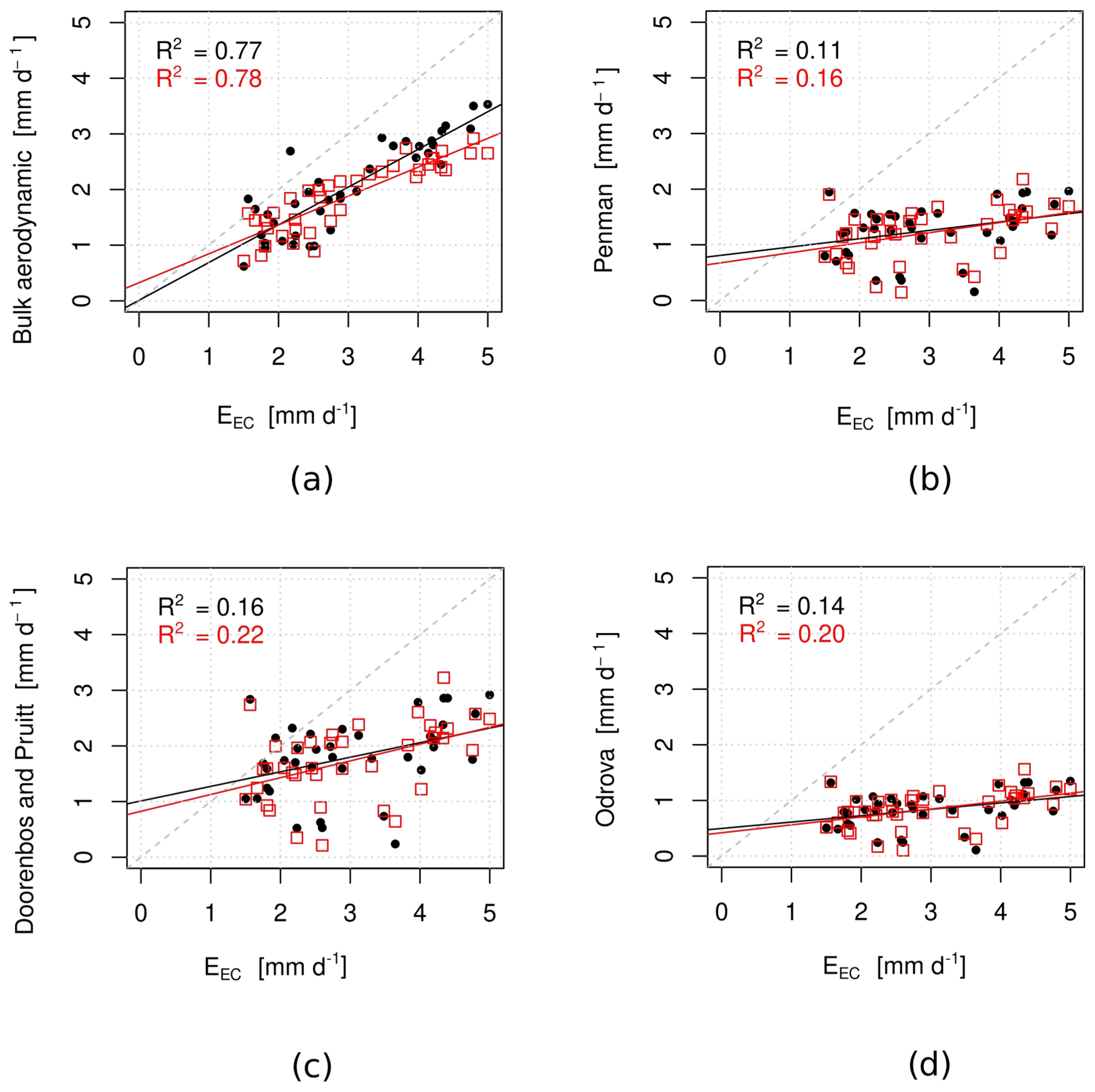
Figure 6Scatter plots of the daily evaporation estimated with the indirect methods (y axis) against the direct EC method (x axis): (a) the bulk-aerodynamic method, (b) Penman (1948), (c) Doorenbos and Pruitt (1975), and (d) Odrova (1979). R2 refers to the determination coefficient. The red dots indicate the estimates of the evaporation with the meteorological parameters measured at the WMO synoptic site Maitri, which is the nearest site to Lake Zub/Priyadarshini. The black dots indicate the estimates of the evaporation made with the meteorological parameters measured at the lake shore (IRGASON site).
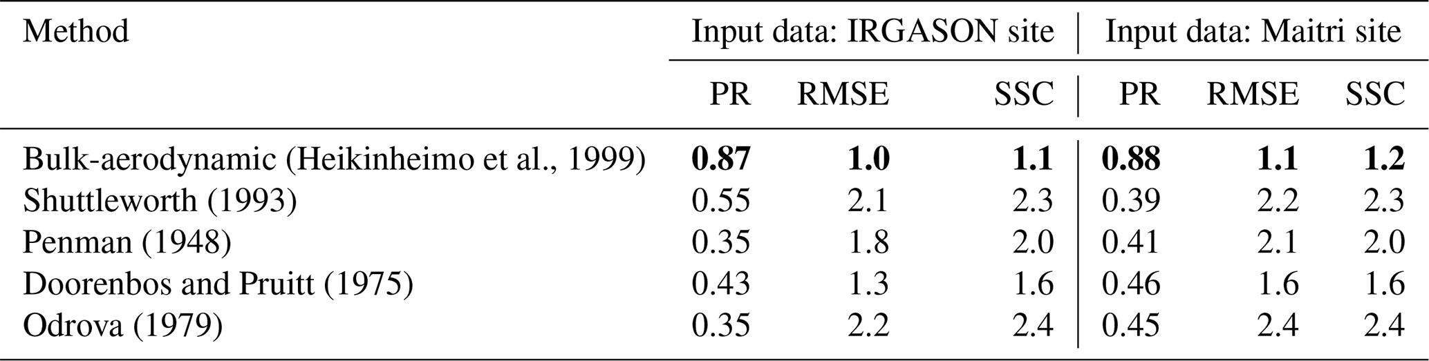
The bulk-aerodynamic method gave the best fit to the EC method according to all criteria (bold notation in Table 4). The mean absolute error of the bulk-aerodynamic method is 0.6 mm d−1, and it is the greatest on those days when the wind speeds are 6–7 m s−1. As one can expect, the efficiency of the empirical equations is poor: the correlation coefficient varied from 0.33 to 0.55, and both the RMSE and SSC criteria indicate the low ability of the methods to estimate daily evaporation. Popov (1979) suggests that any model is applicable for hydrological practice if only . Unfortunately, none of the considered empirical equations can be recommended to calculate the daily evaporation due to big uncertainties inherent in these methods (Fig. 7). Thus, it is needed to derive new empirical coefficients for the combination equation and new mass-transfer coefficients for the bulk-aerodynamic method, allowing better daily evaporation over Lake Zub/Priyadarshini.
Table 4The efficiency of the indirect methods with the Pearson correlation coefficient (PR), the root mean square error (RMSE), and the (SSC) criteria. Bold: best fit to the EC method.
The relationship between evaporation and 2 m wind speed and the saturation deficit was approximated by the formula reading in Table 3. In this formula, two empirical coefficients (A and B) were evaluated from the series of the evaporation (after the EC method) and the wind speed and air temperature observations performed at the Maitri site, which is nearest to Lake Zub/Priyadarshini. The daily series for the period lasting from 1 January to 7 February 2018 was used in the fitting procedure. Figure 7 shows the daily evaporation estimated by the EC method and by the bulk-aerodynamic method with the mass-transfer coefficients applied after Heikinheimo et al. (1999) and a new combination equation with two empirical coefficients fitted from the observations.
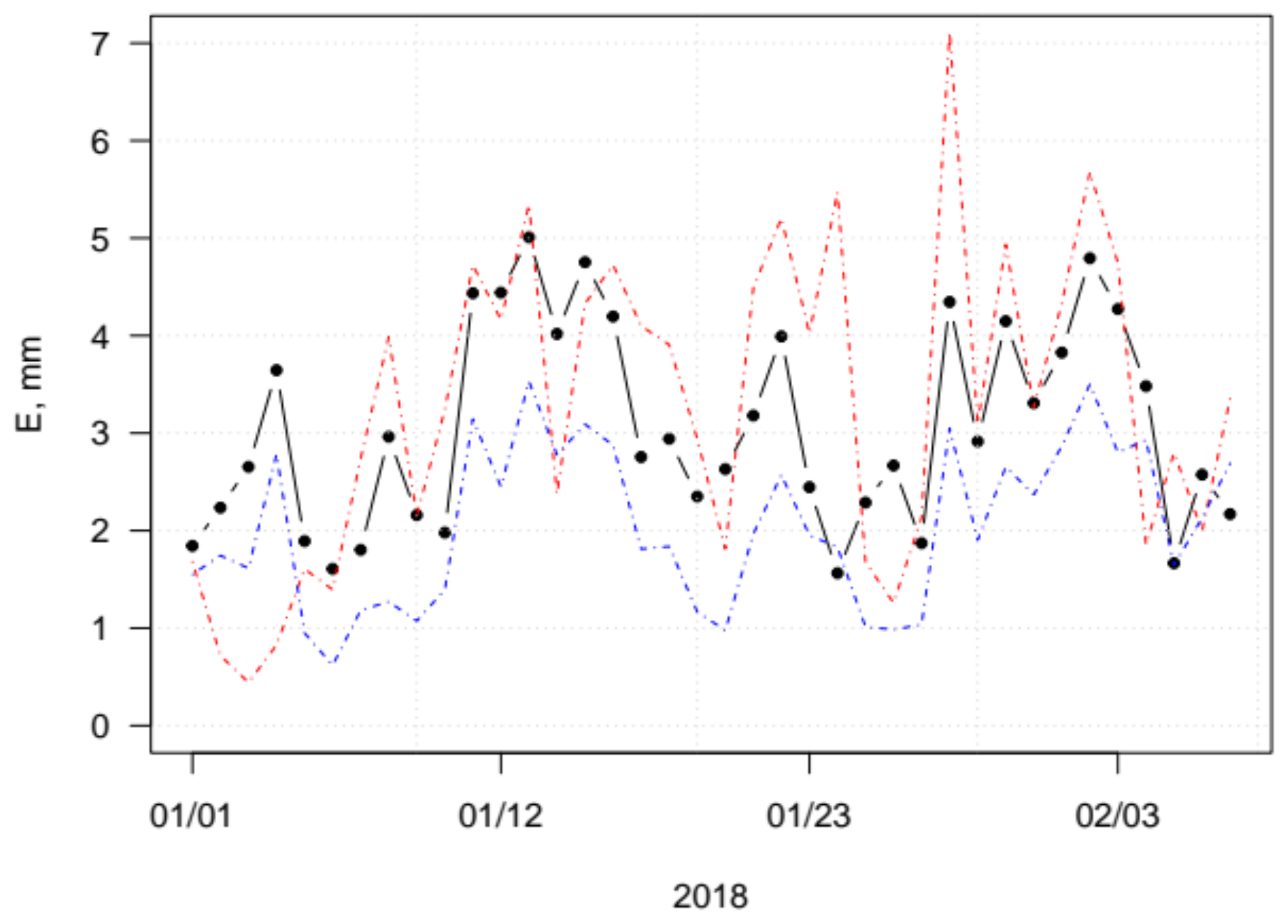
Figure 7The daily time series of evaporation (mm d−1) calculated by the EC method (black), by the bulk-aerodynamic method (blue), and by the new combination equation (red) applying the meteorological measurements at the Maitri site.
The daily evaporation was estimated to be 3.3±1.6 mm d−1 (where the numbers represent the mean and standard deviation, respectively) by the equation ; and the sum of the evaporation for the period 38 d estimated with this formula method differs by less than 10 % from those estimated by the EC method. It is the lowest difference for the indirect methods considered; the Pearson correlation coefficient and the RMSE are estimated to be 0.59 and 1.0, respectively. These scopes allow us to consider this equation the second best among the indirect methods (Table 3), with only the bulk-aerodynamic method showing better results in the estimations of the daily evaporation. The independent data are needed to test the new empirical equation.
The efficiency of the new empirical formula with the independent data was estimated from the wind speed and air temperature measured at the IRGASON site (Fig. 1c). We also used the lake water surface temperature measured at the iButton site for the period of 27 January–7 February 2018 (or 12 d); the daily time series of the evaporation were calculated with this formula, and then they were compared with those estimated after the EC method. The Pearson correlation coefficient and the RMSE are estimated to be 0.68 and 1.3, respectively. The sum of the evaporation for the period of 12 d by this method is over 30 % higher than those estimated by the EC method. It shows that the new combination formula may tend to overestimate the evaporation.
4.2 Impact of katabatic winds on evaporation
The study region is dominated by winds from the south-easterly sector (Fig. 3b). This corresponds to the katabatic winds, which the Coriolis force has turned left from the direct downslope direction. To better understand the impact of katabatic winds, we carried out further analyses on the wind conditions in the study region. We calculated the geostrophic wind fields for each day of the study period from the mean sea level pressure fields estimated from the ERA5 reanalysis. The results demonstrated that the geostrophic (synoptic) wind was mostly from the east, i.e. some 45∘ right from the mean direction of the observed near-surface wind. This deviation angle may partly result from Ekman turning in the atmospheric boundary layer, which over an ice sheet with a rather small aerodynamic roughness may contribute some 20∘, and from the katabatic forcing. In any case, in most cases the observed near-surface winds resulted from the combined effects of synoptic and katabatic forcing, which supported each other. Hence, it is very difficult to robustly distinguish the impact of katabatic forcing on the near-surface winds over the lake.
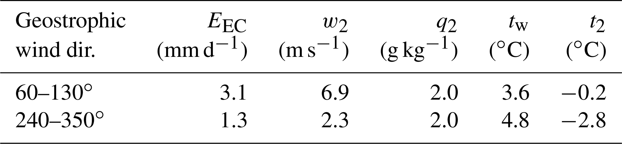
However, the geostrophic wind direction was distinctly different, 240–350∘, on the following days: 6, 8–10, 19, and 25–27 January. These days were related to transient cyclones centred north-west of the lake or high-pressure centres north-east of the region under study. During the days, the wind speed over the lake was strongly reduced (Table 5), as the katabatic and synoptic forcing factors opposed each other. The lake surface temperature was higher than usual, but the air temperature was lower. The latter is partly because, during events when the geostrophic and katabatic forcing factors support each other (sector 60–130∘), the strong wind effectively mixes the atmospheric boundary layer. In stably stratified conditions, which prevail over the ice sheet, vertical mixing results in higher near-surface air temperatures (Vihma et al., 2011). In addition, adiabatic warming during the downslope flow is a major factor contributing to higher air temperatures (Xu et al., 2021). The impact of adiabatic warming is also seen as lower relative humidity in cases when the geostrophic wind is from the sector 60–130∘. Related to the compensating effects of air temperature and relative humidity, the specific humidity was not sensitive to the geostrophic wind direction. The effect of wind speed dominated the effect of the lake surface temperature (which controls qs in Eq. 1), and evaporation was strongly reduced when the geostrophic wind was from the sector 240–350∘ (Table 5).
Table 5The mean values of evaporation (EEC), wind speed (w2), air specific humidity (q2), lake surface temperature (tw), and air temperature (t2) calculated over the days when the geostrophic wind direction was 60–130∘ and when it was 240–350∘.
The katabatic wind was a quasi-persistent feature during the study period, and the major changes in the evaporation were driven by changes in the synoptic-scale wind direction, which affected the local wind speed.
Our study yielded estimates of evaporation over a glacial lake in the summer based on the direct EC measurements during the field experiment lasting 38 d. The daily time series of the evaporation was calculated after the EC method, and then these estimates of evaporation were considered the reference when estimating the uncertainties inherent in the indirect methods (the bulk-aerodynamic method and four combination equations).
Among the indirect methods considered, the lowest level of the uncertainties was in the bulk-aerodynamic method: it underestimated the daily evaporation by over 30 %. We applied the mass-transfer coefficients suggested by Heikinheimo et al. (1999) to calculate the evaporation. We also applied the EC measurements to derive new mass-transfer coefficients for the bulk method; however, the results show two strange aspects: (1) the larger magnitude of the transfer coefficient for moisture than that for momentum and (2) the strong wind dependency of the moisture transfer coefficient. We interpreted the situation to indicate that these strange aspects, contradicting the literature on bulk-transfer coefficients, may arise from three potential factors: (a) evaporation from spray droplets, which is sometimes very large when dry Antarctic air masses are advected over open water (Guest, 2021) but is not accounted for by the bulk formulas; (b) non-local factors affecting turbulence over the lake; or (c) some unidentified error source in the data. By (b) we mean that turbulence over a small lake may be affected not only by the roughness and stratification over the lake surface but also by non-local factors, such as orography of the nunataks and glaciers upwind of the lake. Even if the flux footprint is over the lake, the structure of turbulence may be affected from more remote areas. For example, orography has a strong impact on gustiness of the wind (Agustsson and Olafsson, 2004), which directly affects turbulent mixing, and gravity waves are common downwind of nunataks (Valkonen et al., 2010) with their breaking generating turbulence. Hence, it is not guaranteed that the bulk transfer coefficients based on our data will be useful for estimating evaporation from other Antarctic lakes. Each lake has specific topography/orography around it, and the optimal transfer coefficients may therefore vary a lot between lakes.
We selected four combination equations (by Penman, 1948; Doorenbos and Pruitt, 1975; Odrova, 1979; and Shuttleworth, 1993) to calculate the daily evaporation over the ice-free lake; all equations underestimated the evaporation by 40 %–72 %. The efficiency indexes show that all these methods cannot be recommended for estimation of the evaporation over the ice-free lakes located in Antarctica. We derived the regional empirical coefficients for the combination equation, and it can be potentially used in estimations of the evaporation over the ice-free glacial lakes located in the Schirmacher oasis. The empirical coefficients in the relationship were derived from the evaporation estimated from the EC measurements and from the measurements of wind speed, air temperature, and lake surface temperature. The wind speed and air temperature were measured in two sites (IRGASON and Maitri) during 38 d. The lake surface temperature was measured at two sites with two temperature sensors (HOBO and iButton) for periods of 38 and 14 d. We used the measurements of wind speed and air temperature at the Maitri site, the lake's surface temperature measured by the HOBO, and daily evaporation by the EC method to derive the empirical coefficients in the relationship. Then, we estimated the evaporation using the newly derived relationship for a period of 12 d with the wind speed and air temperature measured at the IRGASON site and also the lake's surface temperature measured by the iButton. However, the measured evaporation by the EC method during the same period (12 d) was only possible for the comparison of the results; therefore the estimations of the efficiency for the new relationship are not fully independent. Therefore we would not suggest applying these coefficients as the regional references without further analysis. In this study, we did not estimate the evaporation using the energy balance method but plan to further evaluate the uncertainties inherent also in this method while estimating the evaporation over the glacial lakes located in Antarctica.
At monitoring sites, evaporation over lakes is in practice measured with evaporation pans, which are not fully applicable in polar regions. The EC measurements require specific equipment that is not always possible to deploy and operate in the remote Antarctic continent. Hence, evaporation (or sublimation) over lakes is usually estimated only indirectly on the basis of regular or campaign observations or numerical model experiments. There are only a few studies of evaporation over lakes located in Antarctica. Borghini et al. (2013) propounded estimates of evaporation over a small endorheic lake located on the shore of Wood Bay, Victoria Land, East Antarctica (70∘ S). This lake is of 0.8 m depth, and by the early 2000s its surface area has decreased to half of the value in the late 1980s. The lake is of the landlocked type, and Borghini et al. (2013) used the method by Shuttleworth (1993) to estimate the evaporation from the lake surface during a couple of weeks in December 2006. They estimated the average daily evaporation as 4.7±0.8 mm d−1; and such an evaporation results in loss of over 40±5 % of the total volume of the lake during the observation period. The lake studied by Borghini et al. (2013) differs from Lake Zub/Priyadarshini, but the daily evaporation rates are of the same order of magnitude, even though one could expect much larger evaporation over the surface of the landlocked lakes than over the surface of the glacial lakes. Our results show that the method by Shuttleworth (1993) underestimates the evaporation of lakes located in the Schirmacher oasis by over 60 %.
Shevnina and Kourzeneva (2017) used two indirect methods to evaluate daily evaporation for two glacial lakes located in the Larsemann Hills oasis, East Antarctica (69∘ S). Lake Progress and Lake Nella/Scandrett are much deeper and larger in volume than Lake Zub/Priyadarshini, and over 30 %–70 % of their catchments are covered by the glacier. The thermal regime of these glacial lakes is also different: Lake Nella/Scandrett and Lake Progress partially lose their ice cover in austral summers when their surface water temperature is 4.5–5.0 ∘C, which is lower than the water temperature over the surface of Lake Zub/Priyadarshini. The daily evaporation was estimated to be 1.8 and 1.4 mm d−1 on the basis of the energy budget method (Mironov et al., 2005) and by the equation of Odrova (1979), respectively. Shevnina and Kourzeneva (2017) concluded that daily evaporation over glacial lakes is underestimated by both of these indirect methods. Our results prove that the uncertainties inherent in the method by Odrova (1979) are the largest among other considered methods.
Faucher et al. (2019) evaluated the evaporation (sublimation) over the surface of the glacial lake Untersee, Dronning Maud Land, East Antarctica (71∘ S). Untersee is perennially frozen year-round; this lake is directly attached to the continental ice sheet, not being the landlocked lake as given by the authors. The evaporation over the lake surface was estimated based on 2 years of measurements by sticks installed on the lake's surface. The water losses from the ice-covered surface of the lake due to sublimation (evaporation) were from 400 to 750 mm yr−1, and the daily evaporation from the lake surface was approximately 1.1–2.1 mm d−1; however the uncertainties inherent in measurements by sticks are not known, and they also need to be quantified in future study.
Lake Zub/Priyadarshini has been given a water supply of the Maitri scientific base which is operated year-round, and therefore the station's managers need to understand its water budget (Dhote et al., 2021). The discrepancies in the lake's water budget depend on the uncertainties inherent in methods used to estimate the lake's budget components, including the evaporation over the lake's surface. In this study, the evaporation is calculated with the empirical equation using the observations collected at the Maitri site. The sum of the evaporation over the lake surface was estimated to be 167 mm for 2 summer months in 2018 (January and February); this is about 2.8 mm d−1, and this estimate is close to those based on the EC method given in this study.
This study focused on the summertime evaporation over a glacial lake located in the Schirmacher oasis, East Antarctica. Over 65 000 glacial lakes were detected in the coastal region via satellite remote sensing in austral summer 2017, and most of them were spread over the ice shelf and the margins of the continental ice sheet (Stokes et al., 2019). The total area of glacial lakes in the vicinity of the Schirmacher oasis was over 72 km2 in January 2017 (Fig. 8), and the two largest glacial lakes were of a similar size to the Schirmacher oasis itself. During warm periods, a high number of glacial lakes (or melt ponds) are recognized over the margins of the Greenland ice sheet (How et al., 2021), and melt ponds are also very common on the surface of Arctic sea ice (Lu et al., 2018). The glacial lakes may exist over the snow-/ice-covered surface for 1–3 months, and their presence has changed land cover properties and affected the surface heat budget. A proper description of land cover is a crucial element of numerical weather prediction (NWP) and climate models, where the overall characteristics of land cover are represented by the surfaces covered by ground, whether vegetation, urban infrastructure, water (including lakes), bare soil, or other. Various parameterization schemes (models) are applied to describe the surface–atmosphere moisture exchange and surface radiative budget (Viterbo, 2002). Lakes have been recently included in the surface parameterization schemes of many NWP models (Salgado and Le Moigne, 2010; Balsamo et al., 2012) with known external parameters (location, mean depth) available from the Global Lake Database (GLDB; Kourzeneva, 2010). The newest version of the GLDB includes glacial lakes in Antarctica (Toptunova et al., 2019). In future studies, it is important to understand how glacial lakes affect the regional air moisture transport over the polar regions and local weather.
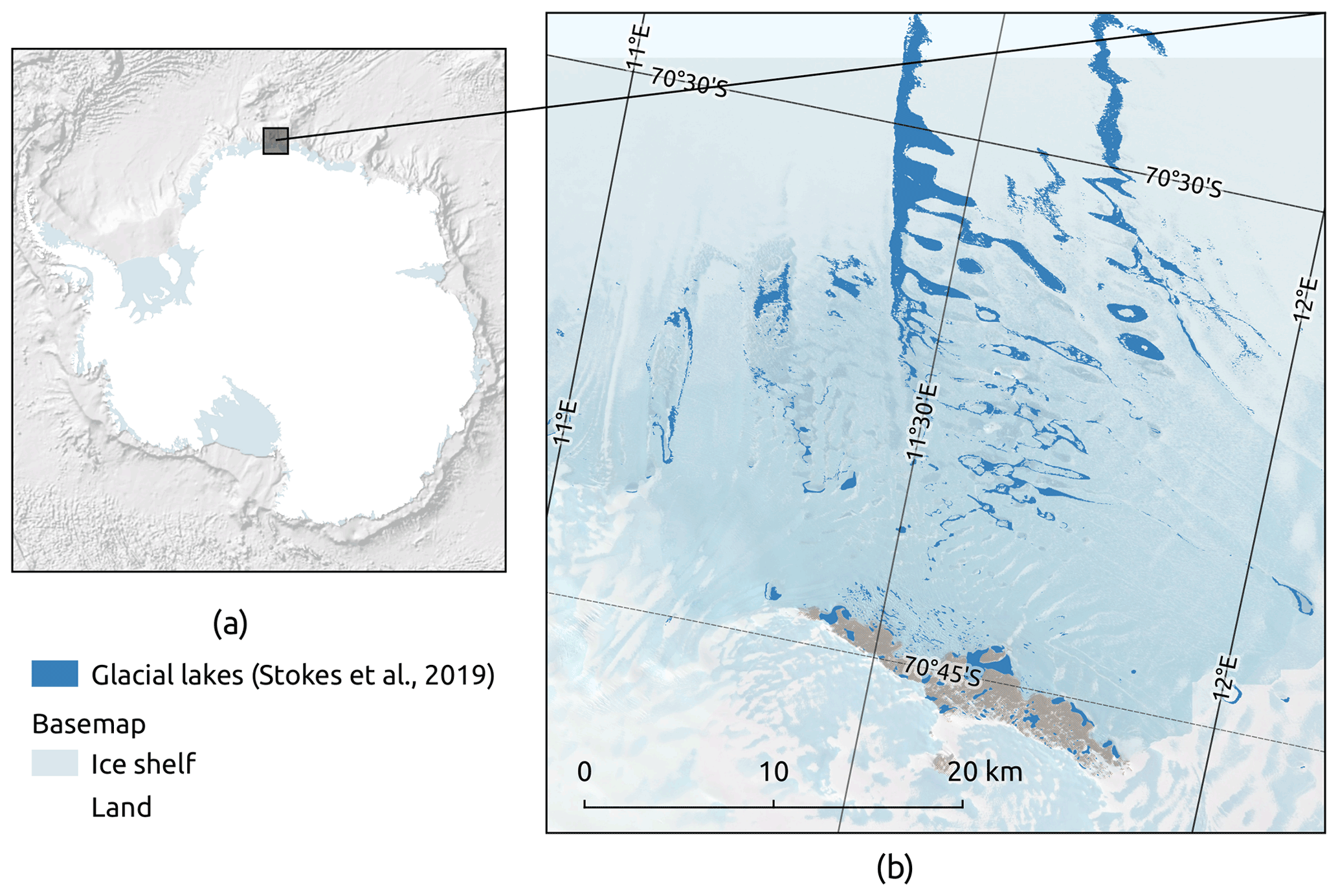
Figure 8The glacial lakes over the surface of an ice shelf in the vicinity of the Schirmacher oasis, East Antarctica. The Antarctic basemap data is provided by Matsuoka et al. (2018).
Estimates of evaporation are available from atmospheric reanalyses which share results of simulations performed by NWP models. As for other reanalyses, ERA5 does not assimilate any evaporation observations, and the evaporation is based on 12 h forecasts of an NWP model by applying the bulk-aerodynamic method. The results naturally depend on the presentation of the Earth's surface in ERA5, and in Dronning Maud Land, the surface type is ice and snow with no lakes. Therefore, the estimate of evaporation does not include evaporation from liquid water surfaces. We also estimated the daily evaporation from ERA5, and the results suggest that the evaporation during summer (December 2017–February 2018) was 0.6 mm d−1. This is only one-fifth of the evaporation estimated with the direct EC method.
Naakka et al. (2021) estimated the evaporation over the Antarctic region from the ERA5 reanalysis for five domains, including the East Antarctic slope where the Schirmacher oasis is located. There the average daily evaporation in summer is 0.3 mm d−1, and this is reasonable for the ice-/snow-covered surface. In summertime, the presence of liquid water over ice-/snow-covered surface changes the fraction of lakes over the East Antarctic slope, and it is 6 %–8 % of the region in the vicinity of the Schirmacher oasis (Fig. 8). The increasing numbers of glacial lakes over the surface of the East Antarctic slope affect the surface–atmosphere moisture interactions, and they also change the regional evaporation not accounted for by the numerical weather prediction systems and climate models. We assumed that the 0.3 mm of ERA5 is a fair value for the ice sheet on the East Antarctic slope and that 3 mm is a representative value for glacial lakes, and it may add up to 0.16–0.22 mm for the regional summertime evaporation over the margins of the East Antarctic slope. These numbers seem to be insignificant for the mass balance of the Antarctic ice sheet and ice shelves. However, we suggest more research to better understand the impact of glacial lakes on the surface heat budget and atmospheric moisture transport in the summer.
This study suggested the estimates of summertime evaporation over an ice-free surface of Lake Zub/Priyadarshini applying the direct EC method and the indirect methods, which only need as input a few hydrometeorological parameters monitored at selected sites (e.g. WMO stations). The catchment Lake Zub/Priyadarshini has less than 30 % of its area covered by glaciers, and this results in a specific thermal regime and water budget of the lake where the evaporation is among the major outflow terms. We estimated the evaporation over the ice-free lake surface as 114 mm in the period from 1 January to 7 February 2018 on the basis of the EC method. The evaporation was estimated to be 3.0 mm d−1 in January 2018. The largest changes in daily evaporation were driven by synoptic-scale atmospheric processes rather than local katabatic winds.
This study gave the estimations of the uncertainties inherent in the indirect methods applied to evaluate summertime evaporation over a lake surface. The bulk-aerodynamic method suggests the average daily evaporation to be 2.0 mm d−1, which is 32 % less than the result based on the EC method. Four selected combination equations underestimated the evaporation over the lake surface by over 40 %–72 %. We suggested a new combination equation to evaluate the summertime evaporation of Lake Zub/Priyadarshini from meteorological observations from the nearest site; however, the empirical coefficients derived for the combination equation are specific for Lake Zub/Priyadarshini and not necessarily valid for other Antarctic lakes. The performance of the new equation is better than the performance of the indirect methods considered. We stress the need for measurements of the lake water surface temperature to allow better estimates of the lake water budget and evaporation (sublimation).
The evaporation results were not sensitive to differences in the data collected at the meteorological site nearest to the lake and the site located on the lake shore. Hence, we suggest using the synoptic records at the meteorological site Maitri to evaluate the evaporation over the surface of Lake Zub/Priyadarshini. Field experiments are needed to make analogous comparisons of meteorological conditions between other glacial lakes and the permanent observation stations nearest to them. The water balance terms of glacial lakes (including evaporation) are closely connected to their thermal regime, and coupled thermophysical and hydrological models are needed to predict the amount of water in these lakes. Our results also demonstrated the need to present glacial lakes in atmospheric reanalyses as well as NWPs and climate models. Ignoring them in a lake-rich region, such as the Schirmacher oasis, results in a large underestimation of regional evaporation in the summer.
The eddy covariance method has some errors and uncertainties associated with the nature of the measurement and the instrument system. Therefore, the results need to be treated with special attention. Nevertheless, the complexity of the method, namely the filters and corrections that this method requires (see Sect. 3.3), makes it possible to reduce the errors and uncertainties. According to Aubinet et al. (2012), there are three methods to quantify the total random uncertainty for the eddy covariance method: the paired tower, 24 h differencing, and the model residual. In our study we apply the paired-tower method to evaluate the errors in the IRGASON installed on the shore of Lake Zub/Priyadarsini. The intercalibration experiment lasted from 12 to 25 October 2018, and during this period two IRGASON instruments were deployed on a floating platform in the Alqueva artificial lake located south-east of Portugal.
The floating platform (38.2∘ N, 7.4∘ W) has been operating continuously since April 2017, and in this experiment, two eddy covariance stations (IRGASON) were installed at a height of 2.0 m next to each other and facing the same footprint (Fig. A1). In this experiment, we compare the measurements of the IRGASON of the Finnish Meteorological Institute (FMI) to those collected by the IRGASON of the Institute of Earth Sciences (ICT), University of Évora. Taking advantage of the fact that both instruments are identical, the settings were set exactly the same. The standard gas zero and span calibration was performed before the experiment. The raw measurements from both instruments were post-processed applying the algorithm given in Potes et al. (2017). This allows precise estimates of random instrument uncertainty, rather than of total random uncertainty, which demands that both instruments are in the same area but with different footprints (Dragoni et al., 2007).
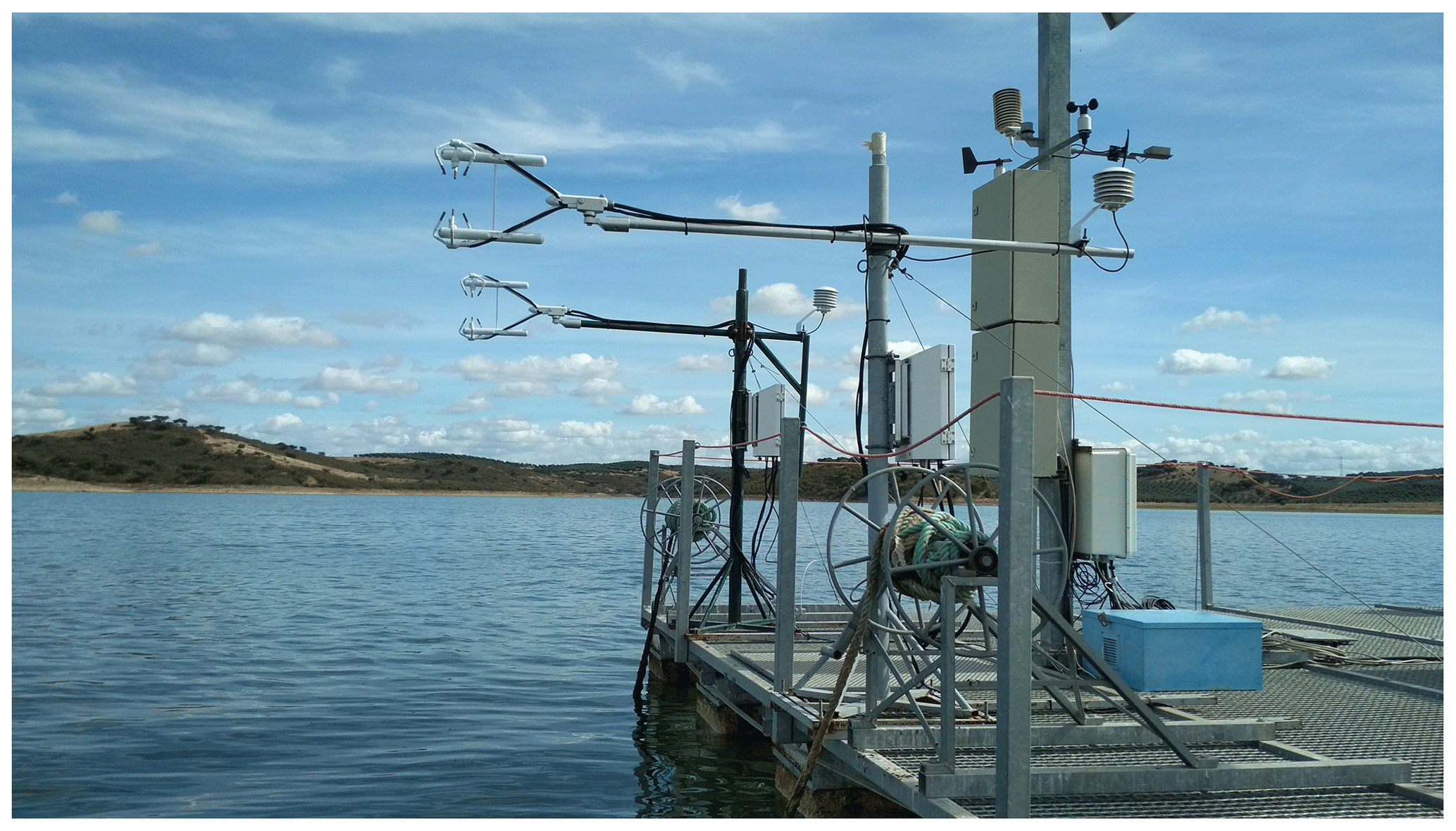
Figure A1The instruments installed in Alqueva reservoir (Portugal) for the intercalibration. The left instrument belongs to the Institute of Earth Sciences, University of Évora, and the instrument on the right belongs to the Finnish Meteorological Institute.
Figure A2 shows a scatter plot between the 30 min evaporation evaluated from the measurements of two instruments during the intercomparison campaign that took place in Alqueva reservoir. The correlation coefficient between the evaporation calculated by the two IRGASON instruments is over 0.98, and this suggests strong agreement between the measurements. Figure A3 presents the frequency distribution of the 30 min evaporation random instrument uncertainty (εF) during the intercomparison campaign (see Eq. 9 from Dragoni et al., 2007). The random instrument error in the 30 min evaporation, estimated as the standard deviation of the evaporation random instrument uncertainty (εF), is 0.004324 mm. Thus, in relative terms, the intercomparison campaign allows obtaining an estimate of a random instrument error of 7.0 %. This value is below other studies presented by several authors, namely Eugster et al. (1997), who used the same approach of the paired towers in Alaskan tundra, and obtained 9 % for latent heat flux; Finkelstein and Sims (2001), who present a value between 14 % and 35 % for latent heat flux in forest and agricultural sites; and Salesky et al. (2012), who found typical errors of 10 % for heat flux.
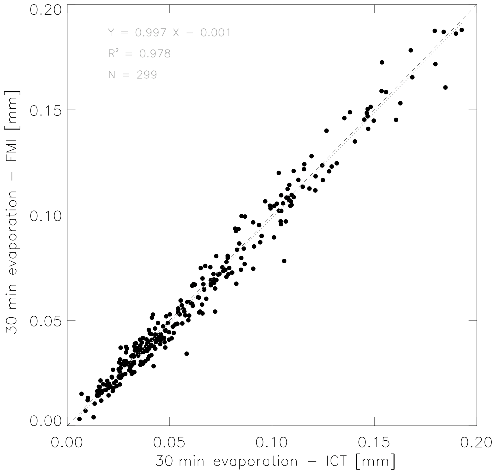
Figure A2Scatter plot between 30 min evaporation from both instruments: the y axis shows the values estimated after the measurements by the IRGASON of the FMI, and the x axis shows the values after the measurements of the IRGASON of the ICT.
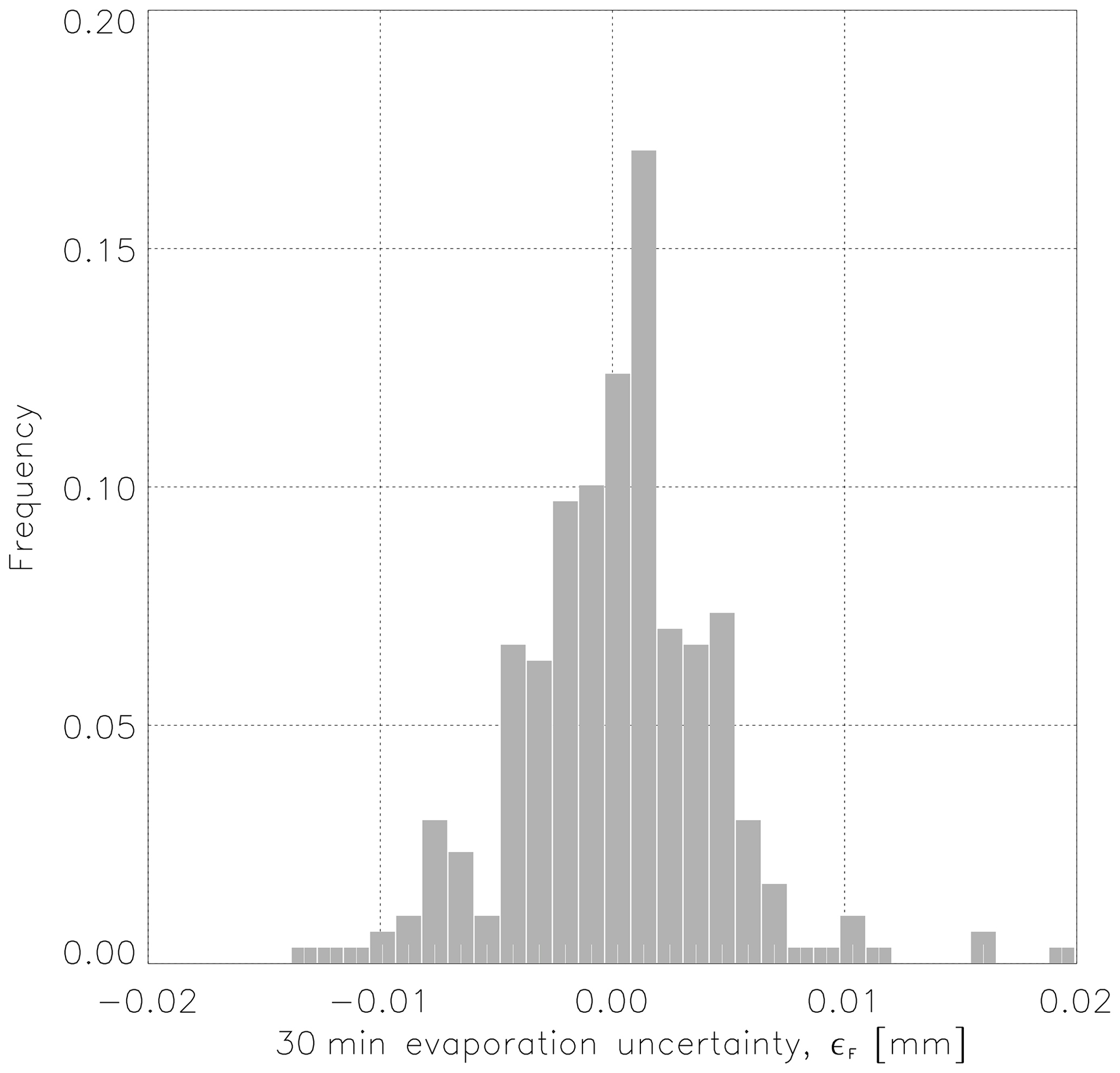
Figure A3Frequency distribution of the 30 min evaporation random instrument uncertainty (εF).
The data and code used in this study are available in the Supplement. We also used two datasets stored at Zenodo: https://doi.org/10.5281/zenodo.3469570 (Shevnina, 2019a) and https://doi.org/10.5281/zenodo.3467126 (Shevnina, 2019b).
Elena Shevnina provided the calculation of the evaporation with the combination equations in Table 3 (combination_equations_results.csv) and the code (results_code.r). Miguel Potes provided the data post-processed by the EC method (20180101_20180207_EC_FLUX.txt). Timo Vihma provided the calculations performed by the bulk-aerodynamic method (Bulk_method_results_Irgason_input.txt and Bulk_method_results_Maitri_input.txt). Pankaj Ramji Dhote provided the meteorological data measured at the Maitri site (Meteorological_Parameters_Summer_2017-18.xlsx). Tuomas Naakka provided the series of the daily evaporation from the ERA5 reanalysis at the grid node nearest to the Novo meteorological site (Evaporation_Schirmacher_Oasis_from_ERA5.csv). The supplement related to this article is available online at: https://doi.org/10.5194/tc-16-3101-2022-supplement.
ES collected the data in the field experiment 2017–2018 and calculated the evaporation applying the combinational equations, their uncertainties, and efficiency indexes. MP supervised the EC measurements in the field; then he calculated the evaporation applying the EC method, and he analysed the data collected during the intercalibration campaign. TV contributed to the estimations of evaporation applying the bulk-aerodynamic method. TN contributed with analyses of evaporation based on ERA5. TV and TN performed the analysis of the impact of the katabatic winds. PRD and PKT contributed with the analysis of the meteorological observations at the Maitri site. All authors contributed to writing of the manuscript.
The contact author has declared that none of the authors has any competing interests.
Publisher's note: Copernicus Publications remains neutral with regard to jurisdictional claims in published maps and institutional affiliations.
This article is part of the special issue “Modelling inland waters in a changing climate (GMD/ESD/TC inter-journal SI)”. It is a result of the 6th Workshop on Parameterization of lakes in Numerical Weather Prediction and Climate Modelling, Toulouse, France, 22–24 October 2019.
The intercalibration campaign in Portugal was partially funded by the COST Action ES1404. The measurement campaigns were supported by the Finnish Antarctic Research Program, the Russian Antarctic Expedition, and the Indian Antarctic Programme. We thank Daniela Franz, Ekaterina Kourzeneva, and Rui Salgado for the discussions during the 5th and 6th Workshops on Parameterization of Lakes in Numerical Weather Prediction and Climate Modelling (October 2017, Berlin, Germany, and October 2019, Toulouse, France). We thank the participants of three scientific conferences – “Comprehensive Research of the Natural Environment of the Arctic and Antarctica”, St. Petersburg, Russia, 2–4 March 2020; “Arctic Science Summit Week” Lisbon, Portugal, 16–26 May 2021, online; and the annual general assembly of the European Geosciences Union (EGU), Vienna, Austria, 23–27 May 2022 – for their questions and comments. Our special thanks go to Alexander Piskun, who shared with us his private collection of bulletins of the Soviet Antarctic Expedition (1960–1986). We are grateful to the Indian Space Research Organisation and National Centre for Polar and Ocean Research (Goa) for constant support and encouragement during this work. We thank Sebastiano Piccolroaz and the two anonymous referees for their fruitful comments and suggestions allowing improvement of the manuscript.
This research has been supported by the Academy of Finland (grant no. 304345), the EU-funded PolarRES project (grant no. 101003590), the EU-funded ALOP project (grant no. ALT20-03-0145-FEDER-000004), and the Fundação para a Ciência e Tecnologia (grant nos. UIDB/04683/2020 and UIDP/04683/2020).
This paper was edited by Sebastiano Piccolroaz and reviewed by two anonymous referees.
Agustsson, H. and Olafsson, H.: Mean gust factors in complex terrain, Meteorol. Z., 13, 149–155, 2004.
Antarctic station catalog: Council of Managers of National Antarctic Programs (COMNAP), Christchurch, New Zealand, 86 pp., 2017.
Arthur, J. F., Stokes, C. R., Jamieson, S. S. R., Carr, J. R., and Leeson, A. A.: Distribution and seasonal evolution of supraglacial lakes on Shackleton Ice Shelf, East Antarctica, The Cryosphere, 14, 4103–4120, https://doi.org/10.5194/tc-14-4103-2020, 2020.
Asthana, R., Shrivastava, P. K., Srivastava, H. B., Swain, A. K., Beg, M. J., and Dharwadkar, A.: Role of lithology, weathering and precipitation on water chemistry of lakes from Larsemann Hills and Schirmacher Oasis of East Antarctica, Adv. Polar Sci., 30, 35–51, https://doi.org/10.13679/j.advps.2019.1.00035, 2019.
Aubinet M., Vesala, T., Papale, D. (Eds): Eddy Covariance: A Practical Guide to Measurement and Data Analysis, ISBN 978-94-007-2350-4e-ISBN, https://doi.org/10.1007/978-94-007-2351-1, 2012.
Balsamo, G., Salgado, R., Dutra, E., Boussetta, S., Stockdale, T., and Potes, M.: On the contribution of lakes in predicting near-surface temperature in a global weather forecasting model, Tellus A, 64, 15829, https://doi.org/10.3402/tellusa.v64i0.15829, 2012.
Bell, R., Chu, W., Kingslake, J., Das, I., Tedesco, M., Tinto, K. J., Zappa, C. J., Frezzotti, M., Boghosian, A., and Lee, W. S.: Antarctic ice shelf potentially stabilized by export of meltwater in a surface river, Nature, 544, 344–348, https://doi.org/10.1038/nature22048, 2017.
Bell, R., Banwell, A., Trusel, L., and Kingslake, J.: Antarctic surface hydrology and impacts on the ice-sheet mass balance, Nat. Clim. Change, 1044–1052, https://doi.org/10.1038/s41558-018-0326-3, 2019.
Blanken, P. D., Rouse, W. R., Culf, A. D., Spence, C., Boudreau, L. D., Jasper, J. N., Kochtubajda, B., Schertzer. W.M., Marsh, P., and Verseghy, D.: Eddy covariance measurements of evaporation from great slave Lake, northwest territories, Canada, Water Resour. Res., 36, 1069–1077, https://doi.org/10.1029/1999WR900338, 2000.
Boisvert, L., Vihma, T., and Shie, C. L.: Evaporation from the Southern Ocean estimated on the basis of AIRS satellite data, J. Geophys. Res.-Atmos., 125, e2019JD030845, https://doi.org/10.1029/2019JD030845, 2020.
Borghini, F., Colacevich, A., Loiselle, S. A., and Bargagi, R.: Short-term dynamics of physico-chemical and biological features in a shallow, evaporative antarctic lake, Polar Biol., 36, 1147–1160, https://doi.org/10.1007/s00300-013-1336-2, 2013.
Bormann, P. and Fritzsche, D.: The Schirmacher Oasis, Queen Maud Land, East Antarctica, and Its Surroundings, Justus Perthes Verlag Gotha, Darmstadt, 448 pp., 1995.
Boronina, A. S., Popov, S. V., and Pryakhina, G. V.: Hydrological characteristics of lakes in the eastern part of the Broknes Peninsula, Larsemann Hills, East Antarctica, Led i Sneg, 59, 39–48, https://doi.org/10.15356/2076-6734-2019-1-39-48, 2019 (in Russian).
Braun, M., Saurer, H., Vogt, S., Simões, J. C., and Goßmann, H.: The influence of large-scale atmospheric circulation on the surface energy balance of the King George Island ice cap, Int. J. Climatol., 21, 21–36, https://doi.org/10.1002/joc.563, 2001.
Brunke, M. A., Fairall, C. W., Zeng, X., Eymard, L., and Curry, J. A.: Which bulkaerodynamic algorithms are least problematic in computing ocean surface turbulent fluxes?, J. Climate, 16, 619–635, https://doi.org/10.1175/1520-0442(2003)016<0619:WBAAAL>2.0.CO;2, 2003.
Brutsaert, W.: Evaporation into the atmosphere – theory, history and applications, D Reidel Publishing Company, Dordrecht, Holland, 299 pp., 1982.
Burba, G.: Eddy Covariance Method for Scientific, Industrial, Agricultural, and Regulatory Applications: A Field Book on Measuring Ecosystem Gas Exchange and Areal Emission Rates, LI-COR Biosciences, Lincoln, NE, USA, 331 pp., 2013.
Businger, J. A., Wyngaard, J. C., Izumi, Y., and Bradley, E. F.: Flux-Profile Relationships in the Atmospheric Surface Layer, J. Atmos. Sci., 28, 181–189, https://doi.org/10.1175/1520-0469(1971)028<0181:FPRITA>2.0.CO;2, 1971.
Chebotarev, A. I.: Hydrology, Hydrometizdat, Leningrad, 544 pp., 1975 (in Russian).
Dhote, P. R., Thakur, P. K., Shevnina, E., Kaushik, S., Verma, A., Ray, Y., and Aggarwal, S. P.: Meteorological parameters and water balance components of Priyadarshini Lake at the Schirmacher Oasis, East Antarctica, Polar Sci., 30, 100763, https://doi.org/10.1016/J.POLAR.2021.100763, 2021.
Doorenbos, J. and Pruitt, W. O.: Crop water requirements, FAO Irrigation and Drainage Paper No. 24 FAO Rome, 179 pp., 1975.
Dragoni, D., Schmid, H. P., Grimmond, C. S. B., Loescher, H. W.: Uncertainty of annual net ecosystem productivity estimated using eddy covariance flux measurements, J. Geophys. Res.-Atmos., 112, D17102, https://doi.org/10.1029/2006JD008149, 2007.
Ellehoj, M. D., Steen-Larsen, H. C., Johnsen, S. J., and Madsen, M. B.: Ice-vapor equilibrium fractionation factor of hydrogen and oxygen isotopes: Experimental investigations and implications for stable water isotope studies, Rapid Commun. Mass Spectrom., 27, 2149–2158, 2013.
Eugster, W., McFadden, J. P., and Chapin, E. S.: A comparative approach to regional variation in surface fluxes using mobile eddy correlation towers, Bound.-Lay. Meteorol., 85, 293–307, 1997.
Faucher, B., Lacelle, D., Fisher, D., Andersen, D., and McKay, C.: Energy and water mass balance of Lake Untersee and its perennial ice cover, East Antarctica, Antarct. Sci., 31, 271–285, https://doi.org/10.1017/S0954102019000270, 2019.
Favier, V., Agosta, C., Genthon, C., Arnaud, L., Trouvillez, A., and Gallée, H.: Modeling the mass and surface heat budgets in a coastal blue ice area of Adelie Land, Antarctica, J. Geophys. Res., 116, F03017, https://doi.org/10.1029/2010JF001939, 2011.
Finch, J. W. and Calver, A.: Methods for the quantification of evaporation from lakes, Prepared for the World Meteorological Organization's Commission for Hydrology, Oxfordshire, UK, 41 pp., 2008.
Finch, J. W. and Hall, R. L.: Estimation of Open Water Evaporation: A Review of Methods, R&D Technical Report W6-043/TR, Environment Agency, Bristol, 155 pp., 2001.
Finch, J. W. and Hall, R. L.: Evaporation from Lakes. Encyclopedia of Hydrological Sciences, Part 4 Hydrometeorology Centre for Ecology and Hydrology, Wallingford, 635–646, 2005.
Finkelstein, P. L. and Sims, P. F.: Sampling error in eddy correlation flux measurements, J. Geophys. Res., 106, 3503–3509, 2001.
Foken, T.: 50 Years of the Monin–Obukhov Similarity Theory, Bound.-Lay. Meteorol., 119, 431–447, https://doi.org/10.1007/s10546-006-9048-6, 2006.
Golubev, G. N.: Hydrology of glaciers. Gidrometeoizdat, Leningrad, 128 pp., 1976 (in Russian).
Gopinath, G., Resmi, T. R., Praveenbabu, M., Pragatha, M., Sunil, P. S., and Rawat, R.: Isotope hydrochemistry of the lakes in Schirmacher Oasis, East Antarctica, Ind. J. Geo Marine Sci., 49, 947–953, 2020.
Guest, P. S.: Inside katabatic winds over the Terra Nova Bay polynya: 2. Dynamic and thermodynamic analyses, J. Geophys. Res.-Atmos., 126, e2021JD034904, https://doi.org/10.1029/2021JD034904, 2021.
Heikinheimo, M., Kangas, M., Tourula, T., Venäläinen, A., and Tattari, S.: Momentum and heat fluxes over lakes Tämnaren and Råksjö determined by the bulk-aerodynamic and eddy-correlation methods, Agric. Forest Meteorol., 98–99, 521–534, https://doi.org/10.1016/S0168-1923(99)00121-5, 1999.
Hersbach, H., Bell, B., Berrisford, P., Hirahara, S., Horányi, A., Muñoz-Sabater, J., Nicolas, J., Peubey, C., Radu, R., Schepers, D., Simmons, A., Soci, C., Abdalla, S., Abellan. X., Balsamo, G., Bechtold, P., Biavati, G., Bidlot, J., Bonavita, M., De Chiara, G., Dahlgren, P., Dee, D., Diamantakis, M., Dragani, R., Flemming, J., Forbes, R., Fuentes, M., Geer, A., Haimberger, L., Healy, S., Hogan, R. J., Hólm, E., Janisková, M., Keeley, S., Laloyaux, P., Lopez, P., Lupu, C., Radnoti, G., de Rosnay, P., Rozum, I., Vamborg, F., Villaume, S., and Thépaut, J.-N.: The ERA5 global reanalysis, Q. J. Roy. Meteor. Soc., 146, 1999–2049, https://doi.org/10.1002/qj.3803, 2020.
Hodgson, D. A.: Antarctic lakes, in: Encyclopedia of Lakes and Reservoirs. Encyclopedia of Earth Sciences Series, Springer, Dordrecht, https://doi.org/10.1007/978-1-4020-4410-6, 2012.
Hoeltgebaum, L. E. B., Diniz, A. L., and Dias, N. L. C.: Intercomparação de sensores de temperatura e umidade relativa para uso em campanha micrometeorológica, Ci. e Nat., Santa Maria v.42, Special Edition: Micrometeorologia, e18, https://doi.org/10.5902/2179460X46565, 2020 (in Portuguese).
Hojjati, E., Mahtabi, G., Taran, F., and Kisi, O.: Estimating evaporation from reservoirs using energy budget and empirical methods: Alavian dam reservoir, NW Iran, Italian J. Agrometeorol., 2, 19–34, https://doi.org/10.13128/ijam-1033, 2020.
Holtslag, A. A. M. and De Bruin, H. A. R.: Applied Modeling of the Nighttime Surface Energy Balance over Land, J. Appl. Meteorol. Climatol., 27, 689–704, 1988.
How, P., Messerli, A., Mätzler, E., Santoro, M., Wiesmann, A., Caduff, R., Lagley, K., Bojesen, M., Paul, F., Kääb, A., and Carrivick J.: Greenland-wide inventory of ice marginal lakes using a multi-method approach, Sci. Rep.-UK, 11, 4481, https://doi.org/10.1038/s41598-021-83509-1, 2021.
Ingole, B. S. and Parulekar, A. H.: Limnoligy of Priyadarshini Lake, Schirmacher oasis, Antarctica, Polar Rec., 26, 13–17, 1990.
Kaup, E.: Development of anthropogenic eutrophication in Antarctic lakes of the Schirmacher Oasis, Verhandlungen Internationale Vereinigung der Limnologie, 29, 678–682, 2005.
Kaup, E. and Haendel, D.: Snow and ice cover of water bodies, in: The Schirmacher Oasis, Queen Maud Land, East Antarctica,, edited by: Bormann, P. and Fritsche, D., Gotha, Justus Perthes Verlag, 279–285, 1995.
Khare, N., Chaturvedi, S. K., Saraswat, R., Srivastava, R., Raina, R., and Wanganeo, A.: Some morphometric characteristics of Priyadarshini water body at Schirmacher Oasis, Central Dronning Maud Land, Antarctica with special reference to its bathymetry, Ind. J. Marine Sci., 37, 435–438, 2008.
Kljun, N., Calanca, P., Rotach, M. W., Schmid, H. P.: A Simple Parameterisation for Flux Footprint Predictions, Bound.-Lay. Meteorol., 112, 503–523, https://doi.org/10.1023/B:BOUN.0000030653.71031.96, 2004.
Klokov, V. D.: Surface melting and liquid water runoff from the Antarctic ice-sheet, Leningrad, Gidrometeoizdat, 126 pp., 1979 (in Russian).
Konovalov, G. V.: Geomorphological description of the Schirmacher oasis and surrounds, B. Sov. Antarct. Exp., 37, 8–13, 1962 (in Russian).
Konstantinov, A. R.: Evaporation Under Natural Conditions, Israel Program for Scientific Translation, Jerusalem, 523 pp., 1968.
Kourzeneva, E.: External data for lake parameterization in numerical Weather Prediction and climate modeling, Boreal Env. Res., 15, 165–177, 2010.
Krass, M. S.: Thermophysics of lakes in Antarctic oases, Reports of the Russian Academy of Science to Antarctic committee, 25, 99–125, 1986 (in Russian).
Launiainen, J. and Vihma, T.: Derivation of turbulent surface fluxes – An iterative flux-profile method allowing arbitrary observing heights, Environ. Softw., 5, 113–114, https://doi.org/10.1016/0266-9838(90)90021-W, 1990.
Leeson, A. A., Shepherd, A., Briggs, K., Howat, I., Fettweis, X., Morlighem, M., and Rignot, E.: Supraglacial lakes on the Greenland ice sheet advance inland under warming climate, Nat. Clim. Change, 5, 51–55, 2015.
Lehnherr, I., St. Louis, V. L., Sharp, M., Gardner, A. S., Smol, J. P., Schiff, L. S., Muir, D. G. G., Mortimer, C. A., Michelutti, N., Tarnocai, C., Pierre, K., Emmerton, C., Wiklund, J. A., Köck, G., Lamoureux, S. F., and Talbot, C. H.: The world's largest High Arctic lake responds rapidly to climate warming, Nat. Commun., 9, 1290, https://doi.org/10.1038/s41467-018-03685-z, 2018.
Levy, J. S., Fountain, A. G., Obryk, M. K., Telling, J., Glennie, C., Pettersson, R., Gooseff, M., and Van Horn, D. J.: Decadal topographic change in the McMurdo Dry Valleys of Antarctica: Thermokarst subsidence, glacier thinning, and transfer of water storage from the cryosphere to the hydrosphere, Geomorphology, 323, 80–97, https://doi.org/10.1016/j.geomorph.2018.09.012, 2018.
Loopman, A., Kaup, E., Klokov, V., Simonov, I., and Haendel, D.: The bathymetry of some lakes of the Antarctic oases Schirmacher and Untersee, in: Limnological Studies in Queen Maud Land (East Antarctic), edited by: Martin, J., Valgus, Tallinn, 6–14, 1988.
Lu, P., Leppäranta, M., Cheng, B., Li, Z., Istomina, L., and Heygster, G.: The color of melt ponds on Arctic sea ice, The Cryosphere, 12, 1331–1345, https://doi.org/10.5194/tc-12-1331-2018, 2018.
Matsuoka, K., Skoglund, A., and Roth, G.: Quantarctica, Norwegian Polar Institute [data set], https://doi.org/10.21334/npolar.2018.8516e961, 2018.
Meredith, M., Sommerkorn, M., Cassotta, S., Derksen, C., Ekaykin, A., Hollowed, A., Kofinas, G., Mackintosh, A., Melbourne-Thomas, J., Muelbert, M. M. C., Ottersen, G., Pritchard, H., and Schuur, E. A. G.: Polar Regions, in: IPCC Special Report on the Ocean and Cryosphere in a Changing Climate, edited by: Pörtner, H.-O., Roberts, D. C., Masson-Delmotte, V., Zhai, P., Tignor, M., Poloczanska, E., Mintenbeck, K., Alegría, A., Nicolai, M., Okem, A., Petzold, J., Rama, B., Weyer, N. M., Cambridge University Press, Cambridge, UK and New York, NY, USA, 203–320, https://doi.org/10.1017/9781009157964.005, 2019.
Mironov, D., Golosov, S., Heise, E., Kourzeneva, E., Ritter, B., Scheider, N., and Terzhevik, A.: FLake – a lake model for environmental applications, in: Proceedings of the 9th Workshop on Physical Processes in Natural Waters, edited by: Folkard, A. and Jones, I., Lancaster University, Lancaster, 73 pp., 2005.
Monin, A. S. and Obukhov, A. M.: Basic laws of turbulent mixing in the surface layer of the atmosphere, Contrib. Geophys. Inst. Acad. Sci. USSR, 151, 187 pp., 1954.
Monteith, J.: Evaporation and the environment, in: 19th Symposium of the Society of Experimental Biology, Cambridge University Press, Cambridge, UK, 205–234, 1965.
Moriasi, D. N., Arnold, J. G., Van Liew, M. W., Bingner, R. L., Harmel, R. D., and Veith, T. L.: Model evaluation guidelines for systematic quantification of accuracy in watershed simulations, T. ASABE, 50, 885–900, https://doi.org/10.13031/2013.23153, 2007.
Mustonen S. (Ed.): Sovellettu hydrologia. Vesiyhdistys, Helsinki, 291–323, 1986 (in Finnish).
Naakka, T., Nygård, T., and Vihma, T.: Air moisture climatology and related physical processes in the Antarctic on the basis of ERA-5 reanalysis, J. Climate, 34, 4463–4480, https://doi.org/10.1175/JCLI-D-20-0798.1, 2021.
Obukhov, A. M.: Turbulence in an Atmosphere with a Non-Uniform Temperature, Bound.-Lay. Meteorol., 2, 7–29, https://doi.org/10.1007/BF00718085, 1946.
Odrova, T.: Hydrophysic of water reservoirs, Leningrad, Gidrometizdat, 312 pp., 1979 (in Russian).
Penman, H. L.: Natural evaporation from open water, bare soil and grass, P. Roy. Soc. Lond. A, 194, 120–145, https://doi.org/10.1098/rspa.1948.0037, 1948.
Phartiyal, B., Sharma, A., and Bera, S. K.: Glacial lakes and geomorphological evolution of Schirmacher Oasis, East Antarctica during Quaternary, Quaternary Int., 23, 128–136, https://doi.org/10.1016/j.quaint.2010.11.025, 2011.
Picard, G., Fily, M., and Gallee, H.: Surface melting derived from microwave radiometers: A climatic indicator in Antarctica, Ann. Glaciol., 46, 29–34, https://doi.org/10.3189/172756407782871684, 2007.
Popov, E. G.: Hydrological forecasts, Leningrad, Gidrometeoizdat, 257 pp., 1979 (in Russian).
Potes, M., Salgado, R., Costa, M. J., Morais, M., Bortoli, D., Kostadinov, I., and Mammarella, I.: Lake–atmosphere interactions at Alqueva reservoir: a case study in the summer of 2014, Tellus A, 69, 1272787, https://doi.org/10.1080/16000870.2016.1272787, 2017.
Ramesh, K. J. and Soni, V. K.: Perspectives of Antarctic weather monitoring and research efforts, Pol. Sci., 18, 183–188, https://doi.org/10.1016/j.Polar.2018.04.005, 2018.
Richter, W. and Borman, P.: Geomorphology of the Schirmacher oasis, in: Bormann, P. and Fritsche, D., The Schirmacher Oasis, Queen Maud Land, East Antarctica, Justus Perthes Verlag, Gotha, 171–206, 1995.
Rodrigues, C. M., Moreira, M., Guimarães, R. C., and Potes, M.: Reservoir evaporation in a Mediterranean climate: comparing direct methods in Alqueva Reservoir, Portugal, Hydrol. Earth Syst. Sci., 24, 5973–5984, https://doi.org/10.5194/hess-24-5973-2020, 2020.
Sahlée, E., Rutgersson, A., Podgrajsek, E., and Bergström, H.: Influence from surrounding land on the turbulence measurements above a Lake, Bound.-Lay. Meteorol., 150, 235–258, https://doi.org/10.1007/s10546-013-9868-0, 2014.
Salesky, S., Chamecki, M., and Dias, N.: Estimating the random error in eddy covariance based fluxes and other turbulence statistics: the filtering method, Bound.-Lay. Meteorol., 144, 113–135, 2012.
Salgado, R. and Le Moigne, P.: Coupling of the FLake model to the Surfex externalized surface model, Boreal Environ. Res., 15, 231–244, 2010.
Shevnina, E.: 3D wind speed and CO2/H2O concentration measurements collected during austral summer 2017/2018 over an ice free surface of a shallow lake located in the Schirmacher oasis, East Antarctica, Zenodo [data set], https://doi.org/10.5281/zenodo.3469570, 2019a.
Shevnina, E.: Water temperature measurements collected during austral summer 2017/2018 on lakes located in the Schirmacher oasis, East Antarctica, Zenodo [data set], https://doi.org/10.5281/zenodo.3467126, 2019b.
Shevnina, E. and Kourzeneva, E.: Thermal regime and components of water balance of lakes in Antarctica at the Fildes peninsula and the Larsemann Hills, Tellus A, 69, 1317202, https://doi.org/10.1080/16000870.2017.1317202, 2017.
Shevnina, E., Kourzeneva, E., Dvornikov, Y., and Fedorova, I.: Retention time of lakes in the Larsemann Hills oasis, East Antarctica, The Cryosphere, 15, 2667–2682, https://doi.org/10.5194/tc-15-2667-2021, 2021.
Shuttleworth, W. J.: Evaporation, in: Handbook of Hydrology, edited by: Maidment, D. R., McGraw-Hill, New York, 4.1–4.53, 1993.
Simonov, I. M.: Oases of East Antarctica, Gidrometeoizdat, 176 pp., 1971 (in Russian).
Simonov, I. M. and Fedotov, V. I.: Ozera oasisa Schimachera [Lakes of the Schirmacher oasis], Informazioni bulletin Sovetskoy Antarcticheskoy Expedicii, 47, 19–23, 1964 (In Rissian).
Sinha, R. and Chatterjee, A.: Thermal structure, sedimentology, and hydro-geochemsitry of Lake Priyadarshini, Schirmacher oasis, Antarctica, Sixteenth Indian Expedition to Antarctica, Scientific Report, Department of Ocean Development, Technical Publication No. 14, 36 pp., 2000.
Sokratova, I. N.: Hydrological investigations in the Antarctic oases, Russ. Meteorol. Hydrol., 36, 207, https://doi.org/10.3103/S1068373911030083, 2011 (in Russian).
Srivastava, A. K., Ingle, P. S., Lunge, H. S., and Khare, N.: Grain-size characteristics of deposits derived from different glacigenic environments of the Schirmacher Oasis, East Antarctica, Geologos, 18, 251–266, https://doi.org/10.2478/v10118-012-0014-0, 2012.
Stannard, D. I. and Rosenberry, D. O.: A comparison of short-term measurements of lake evaporation using eddy correlation and energy budget methods, J. Hydrol., 122, 15–22, https://doi.org/10.1016/0022-1694(91)90168-H, 1991.
Stokes, C. R., Sanderson, J. E., Miles, B. W. J., Jamieson, S. S. R., and Leeson, A. A.: Widespread distribution of supraglacial lakes around the margin of the East Antarctic Ice Sheet, Sci. Rep.-UK, 9, 13823, https://doi.org/10.1038/s41598-019-50343-5, 2019.
Stull, R.: Practical Meteorology: An Algebra-based Survey of Atmospheric Science – version 1.02b, Univ. of British Columbia, 940 pp., 2017.
Tanny, J., Cohen, S., Assouline, S., Lange, F., Grava, A., Berger, D., Teltch, B., and Parlange, M. B.: Evaporation from a small water reservoir: Direct measurements and estimates, J. Hydrol., 351, 218–229, 2008.
Tomasi, C., Cacciari, A.,Vitale, V., Lupi, A.,Lanconelli, C., Pellegrini, A., and Grigioni, P.: Mean vertical profiles of temperature and absolute humidity from a 12-year radiosounding data set at Terra Nova Bay (Antarctica), Atmos. Res., 71, 139–169, https://doi.org/10.1016/j.atmosres.2004.03.009, 2004.
Toptunova, O., Choulga, M., and Kurzeneva, E.: Status and progress in global lake database developments, Adv. Sci. Res., 16, 57–61, https://doi.org/10.5194/asr-16-57-2019, 2019.
Turner, J. and Pendlebury, S. F.: The International Antarctic Weather Forecasting Handbook, British Antarctic Survey, 663 pp., 2004.
Valkonen, T., Vihma, T., Kirkwood, S., and Johansson, M. M.: Fine-scale model simulation of gravity waves generated by Basen nunatak in Antarctica, Tellus, 62A, 319–332, 2010.
Venäläinen, A., Heikinheimo, M., and Tourula, T.: Latent heat flux from small sheltered lakes, Bound.-Lay. Meteorol., 86, 355–377, https://doi.org/10.1023/A:1000664615657, 1998.
Verleyen, E., Hodgson, D. A., Vyverman, W., Roberts, D., McMinn, A., Vanhoutte, K., and Saabe, K.: Modelling diatom responses to climate induced fluctuations in the moisture balance in continental Antarctic lakes, J. Paleolimnol., 30, 195–215, https://doi.org/10.1023/A:1025570904093, 2003.
Verleyen, E., Hodgson, D., Gibson, J., Imura, S., Kaup, E., Kudoh, S., Wever, D. A., Hoshino, T., McMinn, A., Obbels, D., Roberts, D., Roberts, S., Saabe, K., Souffreau C., Tavernier I., van Niewenhuyze, W., van Ranst E., Vindevogel, N., and Vyverman, W.: Chemical limnology in coastal East Antarctic lakes: Monitoring future climate change in centers of endemism and biodiversity, Antarct. Sci., 24, 23–33, https://doi.org/10.1017/S0954102011000642, 2012.
Vickers, D. and Mahrt, L.: Quality control and flux sampling problems for tower and aircraft data, J. Atmos. Ocean. Tech., 14, 512–526, https://doi.org/10.1175/1520-0426(1997)014<0512:QCAFSP>2.0.CO;2, 1997.
Vignon, É., Roussel, M.-L., Gorodetskaya, I. V., Genthon, C., and Berne, A.: Present and future of rainfall in Antarctica, Geophys. Res. Lett., 48, e2020GL092281, https://doi.org/10.1029/2020GL092281, 2021.
Vihma, T., Uotila, J., Cheng, B., and Launiainen, J.: Surface heat budget over the Weddell Sea: buoy results and comparisons with large-scale models, J. Geophys. Res., 107, 3013, https://doi.org/10.1029/2000JC000372, 2002.
Vihma, T., Tuovinen, E., and Savijärvi, H.: Interaction of katabatic winds and near-surface temperatures in the Antarctic, J. Geophys. Res., 116, D21119, https://doi.org/10.1029/2010JD014917, 2011.
Viterbo, P.: A review of parametrization schemes for land surface processes. ECMWF, Reading, England, https://www.ecmwf.int/sites/default/files/elibrary/2002/16960-review-parametrization-schemes-land-surface-processes.pdf (last access: 25 May 2021), 2002.
Williamson, C. E., Saros, J. E., Vincent, W. F., and Smol, J. P.: Lakes and reservoirs as sentinels, integrators, and regulators of climate change, Limnol. Oceanogr., 54, 2273–2282, 2009.
Xu, M., Yu, L., Liang, K., Vihma, T., Bozkurt, D., Hu, X., and Yang, Q.: Dominant role of vertical air flows in the unprecedented warming on the Antarctic Peninsula in February 2020, Commun. Earth Environ., 2, 133, https://doi.org/10.1038/s43247-021-00203-w, 2021.
Zhao, L., Xia, J., Xu, Wang, Z., Sobkowiak, L., and Long, C.: Evapotranspiration estimation methods in hydrological models, J. Geogr. Sci., 23, 359–369, https://doi.org/10.1007/s11442-013-1015-9, 2013.
- Abstract
- Introduction
- The study area, weather, and lakes
- Data and methods
- Results
- Discussion
- Conclusions
- Appendix A: Evaluating the uncertainties in the EC method with the paired-tower method – the intercalibration experiment at Alqueva reservoir, Portugal
- Code and data availability
- Author contributions
- Competing interests
- Disclaimer
- Special issue statement
- Acknowledgements
- Financial support
- Review statement
- References
- Supplement