the Creative Commons Attribution 4.0 License.
the Creative Commons Attribution 4.0 License.
 | 19 Jul 2022
Coherent backscatter enhancement in bistatic Ku- and X-band radar observations of dry snow
Othmar Frey
Irena Hajnsek
The coherent backscatter opposition effect (CBOE) enhances the backscatter intensity of electromagnetic waves by up to a factor of 2 in a very narrow cone around the direct return direction when multiple scattering occurs in a weakly absorbing, disordered medium. So far, this effect has not been investigated in terrestrial snow in the microwave spectrum. It has also received little attention in scattering models. We present the first characterization of the CBOE in dry snow using ground-based and spaceborne bistatic radar systems. For a seasonal snowpack in the Ku-band (17.2 GHz), we found backscatter enhancement of 50 %–60 % (+1.8–2.0 dB) at a zero bistatic angle and a peak half-width at half-maximum (HWHM) of 0.25∘. In the X-band (9.65 GHz), we found backscatter enhancement of at least 35 % (+1.3 dB) and an estimated HWHM of 0.12∘ in the accumulation areas of glaciers in the Jungfrau–Aletsch region, Switzerland. Sampling of the peak shape at different bistatic angles allows estimating the scattering and absorption mean free paths, ΛT and ΛA. In the VV polarization, we obtained m and m at the Ku-band and m and m at the X-band, assuming an optically thick medium. The HH polarization yielded similar results. The observed backscatter enhancement is thus significant enough to require consideration in backscatter models describing monostatic and bistatic radar experiments. Enhanced backscattering beyond the Earth, on the surface of solar system bodies, has been interpreted as being caused by the presence of water ice. In agreement with this interpretation, our results confirm the presence of the CBOE at X- and Ku-band frequencies in terrestrial snow.
- Article
(7817 KB) - Full-text XML
-
Supplement
(12599 KB) - BibTeX
- EndNote


The scattering of electromagnetic waves in any type of medium can be used to characterize some of its structural properties. In radar remote sensing, the scattering characteristics of snow have been intensely studied to derive properties of the snowpack. However, an important effect, the coherent backscatter opposition effect (CBOE), can enhance the radar backscatter return by up to a factor of 2. This effect has rarely been considered in descriptions of the backscatter return from snow in monostatic radar experiments (where the transmitter and the receiver are co-located) because even though the CBOE is present, its magnitude cannot be quantified without a bistatic reference measurement (where the transmitter and the receiver are at separate locations). To fully characterize the CBOE, bistatic radar experiments need to be performed.
1.1 Opposition effects in random media
An opposition effect (also referred to as “opposition peak”, “opposition surge”, “enhanced backscattering”, “hot spot”, and similar) is any phenomenon in which electromagnetic (EM) radiation scattered from a particular medium exhibits an increase in intensity in the direct return direction and its vicinity. Opposition effects occur at a variety of wavelengths and scattering media and are caused by a variety of underlying physical phenomena (Hapke, 2012).
The coherent backscatter opposition effect (CBOE), also referred to as coherent backscatter enhancement or weak localization of electromagnetic radiation, occurs when coherent EM radiation is scattered two or more times within a weakly absorbing, disordered medium. In the direct return direction, where wave vectors of the incident and scattered wave are parallel, the EM waves, traveling through the medium along each possible scattering path, interfere constructively with their time-reversed counterparts (Kuga and Ishimaru, 1984; Tsang and Ishimaru, 1984; Akkermans et al., 1988; Aegerter and Maret, 2009; Hapke, 2012). This constructive interference enhances the backscatter intensity within a very narrow cone of about 0.01–1∘ width by up to a factor of 2, whereas transmission is reduced. In all other directions, scattered waves sum incoherently and form the incoherent background scatter signal. The angular half-width at half-maximum (HWHM) of the CBOE peak is proportional to the ratio of the free-space wavelength λ and the scattering mean free path ΛT (Hapke, 2012, Eq. 9.42). The peak tip can be very sharp when high orders of scattering contribute. The peak becomes rounder, wider, and less intense when absorption and finite sample thickness limit the contribution of multiple scattering (Akkermans et al., 1988, Fig. 7; Van Der Mark et al., 1988, Fig. 20).
The CBOE can occur together with the shadow-hiding opposition effect (SHOE). However, the SHOE requires particles to be large enough to cast sharp shadows within a porous medium (fine dust, vegetation canopy). Particles can then hide their own shadow in the direct return direction (Hapke, 1986; Hapke et al., 1996). In contrast to the CBOE, the SHOE is caused by single scattering, while multiple scattering weakens the SHOE; absorption is not critical. The HWHM of the SHOE peak is given by the ratio of the particle radius to the particle-to-shadow distance or extinction length in the medium (Hapke, 2012, Eq. 9.24). For the surface of the Moon, acting as a prototype for virtually all solar system objects with exposed surfaces, both the CBOE and the SHOE contribute with similar parts to the scattered light in the visible spectrum in the direct return direction (Hapke et al., 1998).
1.2 Observations of the CBOE
Most quantitative measurements of the CBOE that characterize the whole angular width of the peak have been carried out at visible-light wavelengths through laboratory experiments which are easier to realize than radio-frequency field and planetary experiments (Montgomery and Kohl, 1980; Kuga and Ishimaru, 1984; Wolf and Maret, 1985; Van Albada and Lagendijk, 1985; Hapke, 1986; Akkermans et al., 1986; Wolf et al., 1988; Van Albada et al., 1988, 1990; Hapke et al., 1996; Mishchenko et al., 2000). In the context of the Earth's cryosphere, Kaasalainen et al. (2006) investigated and confirmed the presence of 10 %–60 % backscatter enhancement in snow at optical wavelengths (632.8 nm) and interpreted the observed narrow angular peak width of 0.1–1∘ at HWHM as dominated by the CBOE.
In the radio-frequency spectrum, the CBOE is mostly discussed in connection with snow and ice deposits where microwave absorption is weak (Warren and Brandt, 2008; Mätzler and Wegmüller, 1987, 1988). In planetary science, the CBOE was proposed as an explanation for the unusually high radar cross-sections of surfaces of various solar system bodies (Muhleman et al., 1991; Black et al., 2001; Hapke et al., 1993). The CBOE was also discussed as a potential cause of the unusual radar echoes from the Greenland ice sheet (Rignot et al., 1993), although internal reflections were proposed as an alternative explanation (Rignot, 1995). In both of these contexts, additional measurements at small but non-zero bistatic angles were desired (but not feasible), as they would have provided a way to more easily and robustly characterize the effect (Hapke, 1990; Rignot, 1995). Bistatic radar measurements of surfaces of solar system bodies are possible by using an orbiting spacecraft in combination with the deep space network receivers on the Earth (Simpson, 1993; Palmer et al., 2017). However, such experiments require a very specific geometric alignment of the spacecraft's orbit with respect to the Earth and are thus not common. Nevertheless, several experiments have been carried out with the Moon as the target (Yushkova et al., 2018): the Clementine bistatic radar experiment observed an opposition peak in certain areas of the lunar surface. This peak was suggested to be attributable to the CBOE, implying the existence of ice deposits on the surface (Nozette et al., 1996), though other work called the interpretation of the Clementine data into question (Simpson and Tyler, 1999). More recently, the Mini-RF instrument of the Lunar Reconnaissance Orbiter, in concert with Arecibo Observatory's radio telescope acting as the transmitter, detected the opposition surge in certain areas of the lunar surface, again attributed to the presence of near-surface deposits of water ice (Patterson et al., 2017).
In many of these experiments, observation of a backscatter enhancement peak at radio frequencies was interpreted as the CBOE. This interpretation was then used to infer the possible existence of water ice (presumably with a porous or disordered structure so as to elicit the effect) on the surface of the corresponding solar system bodies. Other works considered the CBOE in microwave scattering models of terrestrial snow (Tan et al., 2015) but could not analyze the peak shape of the CBOE. In this work we demonstrate that the existence of snow on the Earth can indeed cause a CBOE. We present a sampling of the peak shape at Ku- and X-band radio wavelengths with ground-based and spaceborne imaging radars.
To characterize the angular peak of backscatter enhancement effects in the radio-frequency spectrum, we used two bistatic radar systems, the ground-based system KAPRI and the spaceborne satellite formation TanDEM-X. For both systems, the transmitter and receiver are placed on independent platforms, and thus the bistatic angle can be varied. The bistatic angle β is defined as the angle between the transmitter, the observed location, and the bistatic receiver. In the exact direct return direction, the bistatic angle is zero and the scattering alignment is called the monostatic configuration.
2.1 Ground-based observations – KAPRI
The Ku-band Advanced Polarimetric Radar Interferometer (KAPRI) is a polarimetric radar system based on the GAMMA Portable Radar Interferometer (GPRI), developed by Gamma Remote Sensing (Werner et al., 2012; Baffelli et al., 2017). It is a ground-based Ku-band frequency-modulated continuous-wave (FMCW) real-aperture radar system, capable of performing fully polarimetric, bistatic measurements. In the bistatic configuration comprised of two synchronized radar instruments with different antenna configurations, the bistatic system offers coverage of areas hundreds of meters wide at a range of several kilometers. The instruments operate at a central frequency of 17.2 GHz (λ=1.74 cm), with a 200 MHz bandwidth. The bistatic configuration and the processing pipeline to generate bistatic single-look complex (SLC) data are detailed in Stefko et al. (2022). A description of the antenna configuration while using a cable synchronization setup can be found in Stefko et al. (2021, Fig. 2).
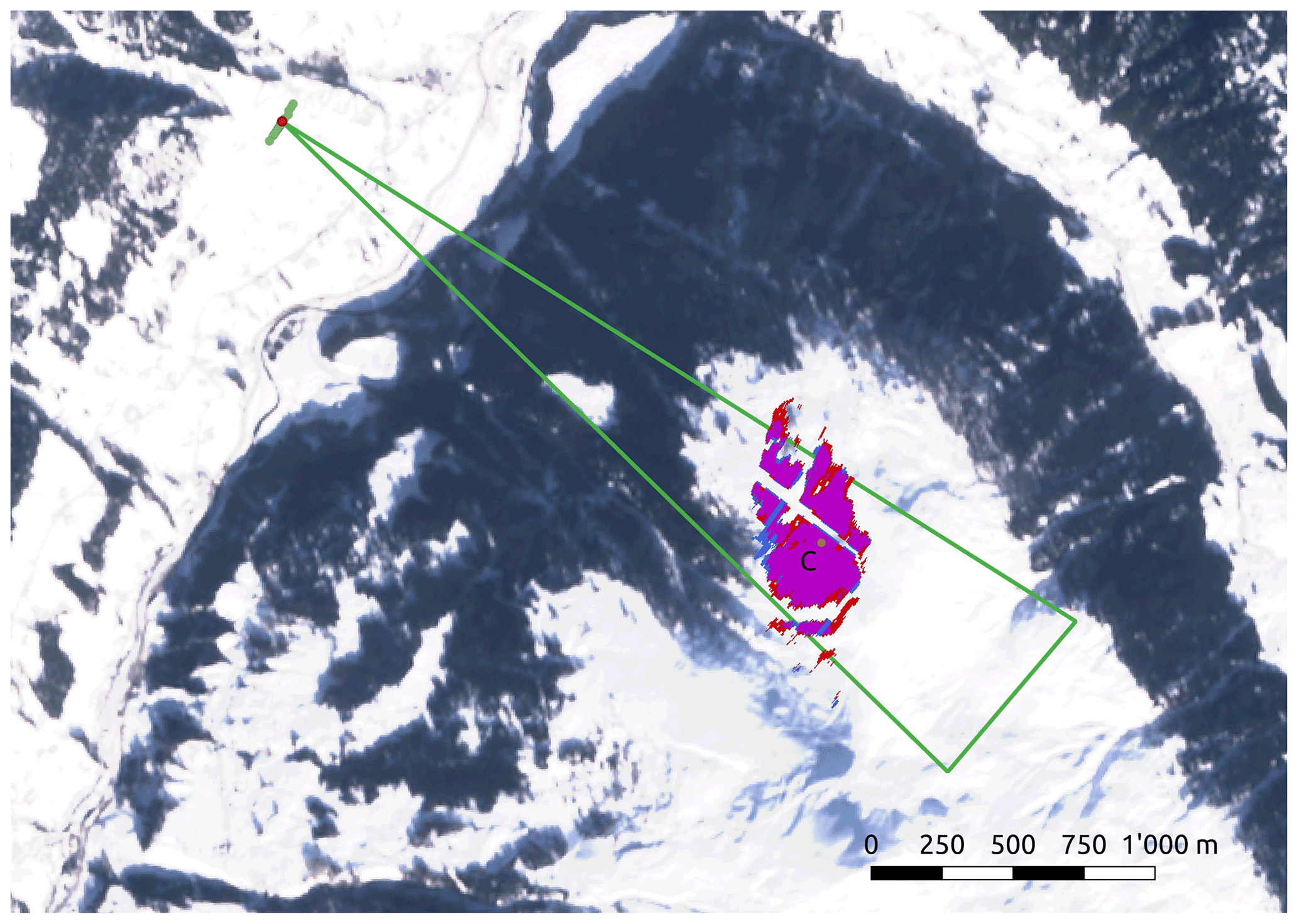
Figure 1Map of the ground-based bistatic radar experiment. The position of the fixed transmitter (red dot) and the different receiver positions (green dots) are marked in the upper left corner and form the bistatic baseline b. The green triangle marks the −3 dB antenna beamwidth of 12∘ of the receiver device. The antennas are oriented towards the snow-covered northwest face of the mountain Rinerhorn, Switzerland. The region of interest (ROI) for the winter and summer seasons is shown in blue and red respectively. Their overlap is shown in purple. C is a reference point for the orientation of the bistatic receiver (see Fig. 4). The hollow line slicing through the ROI masks out metallic beams from a ski lift on the slope. Satellite imagery data: Sentinel-2 on 20 February 2021. Modified Copernicus Sentinel data 2021/Sentinel Hub.
2.1.1 Observation site – Rinerhorn, Davos
For the ground-based experiment (map shown in Fig. 1), the observed region of interest (ROI) was located on the northwestern face of the Rinerhorn peak near Davos, Switzerland. Both devices were located on the valley side opposite the peak, at 46.763∘ N, 9.788∘ E (Fig. 1). The radar location features a straight and relatively flat segment of road approximately 200 m long with unobstructed view of Rinerhorn. The devices were placed at approximately 1620 m altitude, while the ROI altitude spans from 2050 to 2270 m. With this upward-looking observation geometry the vast majority of the ROI area is observed under a shallow local incidence angle larger than 70∘. Problems with multipath interference arising from the upward-looking observation geometry while employing a fan-beam radar system (Lucas et al., 2017) are avoided by placing the instruments on the opposing side of the valley.
We performed two experiments: in summer (5 August 2020), the ROI was covered by low grass. In winter (18 February 2021), the area was completely covered by approximately 1.5 m of seasonal snow. Each measurement began at approximately 08:00 local time, and the total duration of the observations was 3.5 h in summer and 5.5 h in winter. In winter, a snow pit revealed snow temperatures of −10 ∘C at the snow surface and −0.2 ∘C at the bottom of the snowpack (Fig. 2, left). The traditional snow grain size, measured as the mean maximum extent of snow crystals (Fierz et al., 2009), was Dmax=0.3 mm at the surface and 1.5 mm at the base (Fig. 2, right).

Figure 2Snow temperature and grain size in the study area close to point C in Fig. 1 on 18 February 2021. Snow height is 1.55 m.
To select the ROI, a mask fulfilling the following three conditions was applied for each season: (1) include only terrain higher than the treeline at 2050 m altitude. (2) Exclude areas containing non-natural structures (metallic support beams, metal ropes, buildings, corner reflectors). (3) Exclude areas affected by radar shadow, and exclude areas outside of the main beam of the secondary antennas – these areas were detected by applying a threshold to the magnitude of the single-pass interferometric coherence γ of the secondary receiver in the VV channel. In every acquisition in the summer dataset, pixels with γ<0.85 were masked out; in the winter dataset pixels with γ<0.80 were masked out. A sliding window of 5×3 (range×azimuth) pixels was used for coherence estimation. The winter threshold is lower due to lower overall coherence in comparison to summer.
The masks defining the ROI for each season are shown in Fig. 1. They cover practically the same region of the hillside. The acquired calibrated SLC datasets were spatially multilooked using a 5×3 window to obtain the intensity images and analyzed in the radar polar geometry (range×azimuth angle). The intensity value (the hat symbol indicates it is a measured quantity) was computed for every acquisition by averaging the measured intensities of all pixels within the ROI. We analyzed only acquisitions with VV and HH polarization as the cross-polarized signal was too close to the noise floor to provide reliable data.
2.1.2 Device configuration and measurement procedure
The primary (monostatic) transmitter–receiver remained stationary during the experiment (Fig. 3, top) and performed azimuthal sweep acquisitions of the observed area at a range of approximately 2.5 km. The secondary device (bistatic receiver) was moved stepwise to sample bistatic angles between 0.04 and 1.92∘. In winter, the secondary device was mounted on a large sledge (Hornschlitten, Fig. 3, middle). In summer, a wheeled cart was used as a movable radar platform (Fig. 3, bottom). The trajectory of the secondary device is visualized in Fig. 4.
The bistatic angle β was calculated for each position of the secondary receiver S as
The length of the bistatic baseline b is given by the length of the vector between the primary and secondary radar's positions, after projecting it into the plane orthogonal to the line of sight. The line of sight is the vector between the primary radar P and the reference point C in the ROI (see Fig. 4). Its length is dPC=2500 m.
To ensure optimal overlap of the antenna patterns in the ROI, the secondary device was leveled and oriented manually in each position. The pitch and roll angles of the mobile platform with respect to the true vertical direction were measured with a digital spirit level at each measurement point and did not exceed 2∘ in either direction. In the azimuth direction, the device was oriented with a compass and optical viewfinder using a reference point in the center of the ROI (point C in Fig. 1). The estimated precision is 1∘.
The transmit antennas on the primary KAPRI device have a physical horizontal length of 2 m (Fig. 3, top), and thus the bistatic angle at a 2.5 km range differs by ∼0.05∘ between the two edges of the transmit antenna. This imposes a practical limit on the resolution of the sampling of the intensity curve: any variation in intensity within bistatic angles of less than 0.05∘ will be smeared out by the non-zero size of the transmit antennas.
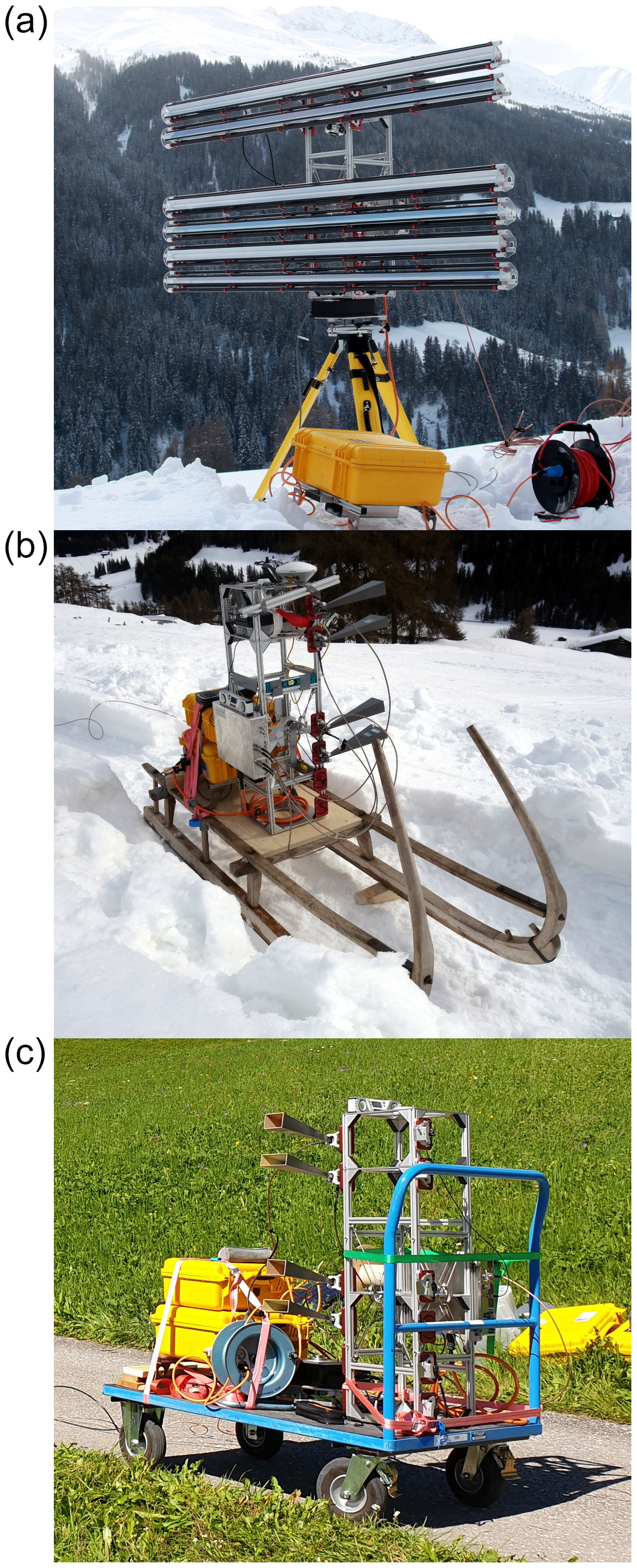
Figure 3(a) Primary KAPRI radar tower (monostatic transmitter–receiver) during the ground-based experiment equipped with narrow-beam traveling-wave antennas. (b) Secondary KAPRI radar tower (bistatic receiver) equipped with horn antennas and deployed on a sledge (Hornschlitten) in winter. (c) Secondary KAPRI tower deployed on a wheeled cart in summer.
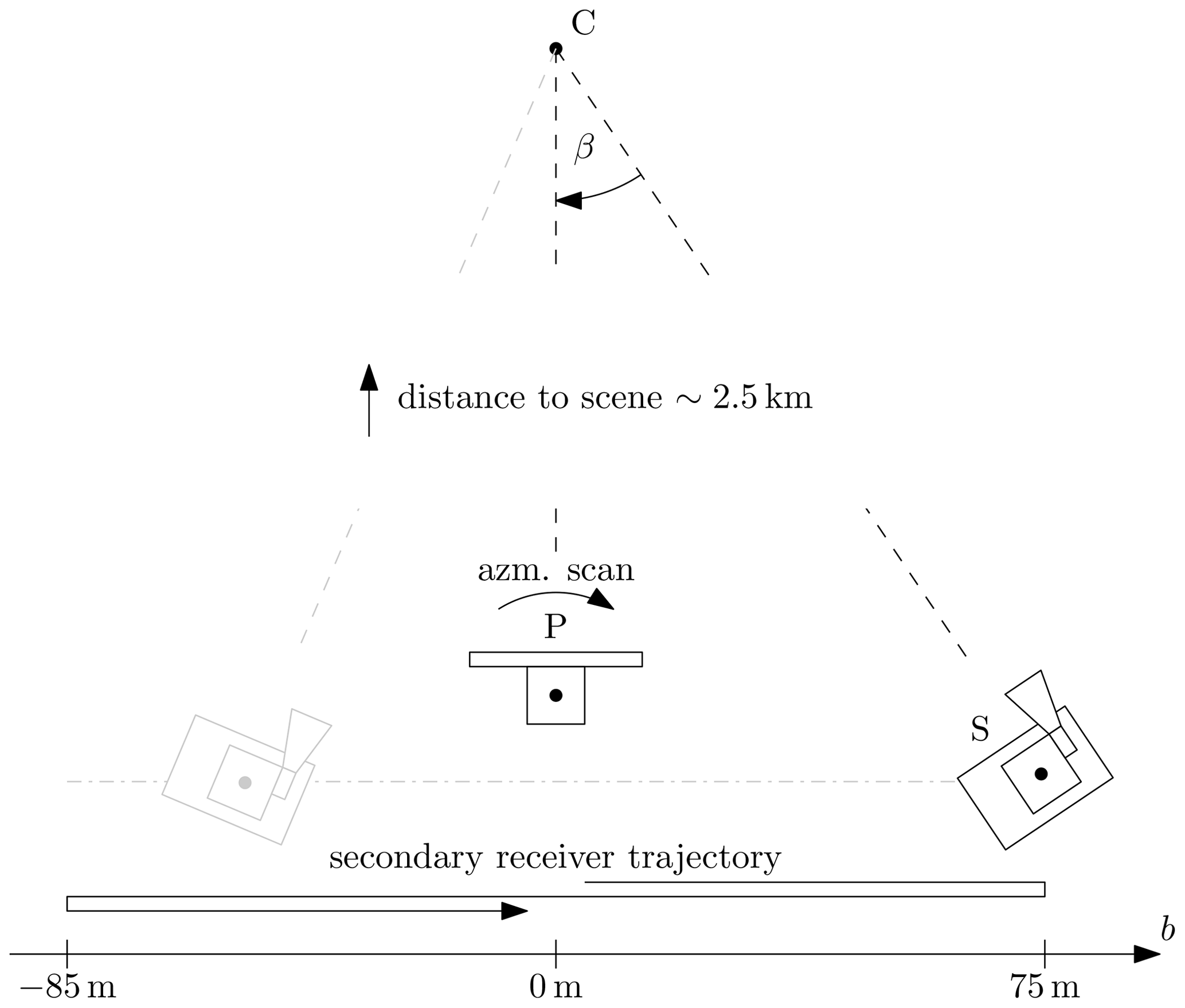
Figure 4Diagram of the ground-based measurement procedure. The stationary, primary device P performs repeated azimuthal scans of the ROI around point C. To sample the scattering response of the ROI under a variety of bistatic angles β, the mobile secondary device S is repositioned in between acquisitions. For both winter and summer experiments, S was placed at bistatic baselines b varying between −85 and +75 m relative to P.
2.1.3 KAPRI – radiometric precision
Three main factors were identified which can affect the radiometric precision of the measurements: temporal drift of the scattering properties in the ROI, the radiometric stability of the bistatic KAPRI system, and the pointing precision of the secondary receiver's antennas.
The trajectory of the bistatic receiver (Fig. 4) was designed to repeatedly increase and decrease the absolute value of the bistatic baseline. This allows detection of any temporal drift of the scattering intensity over the course of the measurement (i.e., on the order of minutes to hours). Drifts would be detected by the different shape of the left and right wing of the intensity curve .
The radiometric stability of KAPRI can be assessed by investigating the monostatic scattering intensity observed by the monostatic device from a reference target (a corner reflector). The maximal detected variation was observed in the HH channel in the winter season, with standard deviation of 16 % relative to the mean value.
For each individual measurement, the beam-pointing direction of the secondary receiver differed by less than 1∘ in the azimuth direction from the ideal central pointing direction towards point C. Due to the antenna pattern of the secondary receiver (Stefko et al., 2022, Fig. 7), an azimuthal misalignment of 1∘ can reduce the signal intensity by not more than ∼1 dB (25 %) at the edge of the “ideal” antenna pattern footprint covering the ROI. However, when considering the total received backscatter from the ROI, this reduction is partially compensated for since the observed backscatter intensity from the other edge of the ROI would necessarily increase.
Due to the limited radiometric stability and the beam-pointing uncertainty, the observed backscatter intensity can thus be expected to vary stochastically with an estimated standard deviation of approximately 20 %, affecting each individual measurement by a significant amount. These effects are difficult to compensate for since there were no reference targets in the scene with a sufficiently high and stable bistatic radar cross-section. For this reason, no a posteriori radiometric calibration was applied to the data. However, the two effects are stochastic in nature and uncorrelated between individual receiver positions, and thus with a sufficiently high number of acquisitions, the enhancement peak should still be detectable, albeit with lower radiometric precision.
2.2 Satellite observations – TanDEM-X
The TanDEM-X satellite formation is the first spaceborne bistatic radar system with an adjustable bistatic baseline. The formation consists of two free-flying synthetic-aperture radar (SAR) satellites, TerraSAR-X and TanDEM-X, orbiting the Earth at about 514 km height in a helix-like formation (Krieger et al., 2007). The two radar instruments operate at the X-band at a central frequency of 9.65 GHz (λ=3.11 cm). Depending on the acquisition mode, both satellites can act as either a transmitter or a receiver or both. In the bistatic mode, the transmit–receive satellite operates in a monostatic observation geometry and the receive-only satellite operates in a bistatic observation geometry.
Since the launch of TanDEM-X in June 2010, the distance between the two satellites has varied by several kilometers. The largest (and smallest) distances were obtained during the TanDEM-X science phase between October 2014 and February 2016 (Hajnsek et al., 2014). To find an area best suited for observation of the CBOE in the X-band, we searched the entire TanDEM-X archive for areas that are covered by deep snow and where long acquisition time series with large bistatic angles are available. Unfortunately, near the poles, bistatic angles are relatively small, making a sufficient sampling of the CBOE peak difficult. At the Equator, the largest bistatic angles of up to 0.35∘ are available but snow is naturally rare. As a best compromise, we not only selected the Jungfrau–Aletsch region in Switzerland but also analyzed the Teram Shehr and Rimo glaciers in the Karakorum (Supplement), where a considerably lower number of acquisitions were available.
2.2.1 Jungfrau–Aletsch region
The Jungfrau–Aletsch region was selected as a TanDEM-X super test site with the aim to acquire as many acquisitions as possible and to explore the scientific value of the bistatic radar mission. Between 2011 and 2019, 118 bistatic acquisitions at two polarizations (VV, HH) were acquired, most of them during winter (Fig. 5). At VH polarization no acquisitions at sufficiently large β values were available. For 104 acquisitions TerraSAR-X acted as the transmitter; for 14 acquisitions TanDEM-X acted as the transmitter. We removed the 14 TanDEM-X acquisitions because they showed slightly different antenna patterns that could not be compensated for through the calibration, especially at HH polarization, because of a too small number of acquisitions. For the remaining 104 acquisitions, bistatic baselines between 65 and 2100 m are available, corresponding to the range β=0.005 to . The incidence angle at the scene center is θ=32∘ (orbit 154, descending). Time-averaged backscatter images of the study area are provided in the Supplement Figs. S2 and S3. Interferometric and polarimetric properties of the dataset were analyzed by Leinss and Bernhard (2021).
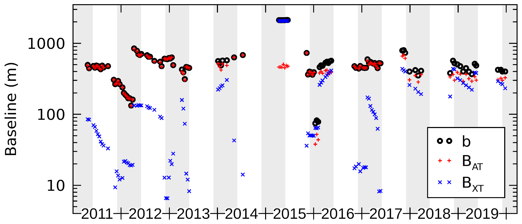
Figure 5Time series of the bistatic baselines b according to Eq. (2) together with along- and across-track baselines BAT and BXT of the TanDEM-X satellite acquisitions of the Jungfrau–Aletsch region. Along-track baselines are adjusted by 30 m due to the satellite motion (see Sect. 2.2.2). Gray shading indicates the period from 1 December until 31 May for which we assume that the firn, present in the accumulation area >3500 m, is completely frozen.
The Jungfrau–Aletsch region is highly glaciated with multiple peaks reaching above 4000 m. Cold firn, several tens of meters deep, is likely present throughout the year: depending on exposition, the transition to temperate firn is at 3400–4000 m, and the upper 15 m of firn experiences seasonal temperature cycles and can freeze in winter (Suter et al., 2001; Suter and Hoelzle, 2002; Jun et al., 2002). At the end of March 2021, snow temperatures of ∘C in the upper 2 m and ∘C at −8 m were measured by Jacqueline Bannwart (personal communication, 2021) at two sites, one at 3380 m altitude (46.5525∘ N, 8.0286∘ E) and one at 3350 m altitude (46.5483∘ N, 8.0323∘ E). At the beginning of March 2022, we measured snow temperatures of ∘C in the upper 2 m and ∘C at −5 m at 3640 m altitude (46.5515∘ N, 8.0062∘ E). Both Bannwart's firn cores as well as our snow pit measurements indicate the presence of an ice layer a few centimeters thick resulting from melt and refreeze during previous summers below the several-meters-thick seasonal snow cover.
The region contains the Great Aletsch Glacier (46.50∘ N, 8.03∘ E), the largest glacier in the European Alps. Its equilibrium line altitude, above which accumulation dominates, is at ∼ 3000 m (Zemp et al., 2007). In the ablation area below, seasonal snow is present. Ice-free areas are dominated by rock and scree. Below 2500 m vegetation dominates with a treeline of 2000 m. For analysis of specific land cover types, we selected the following three regions of interest (ROIs) in the Jungfrau–Aletsch region (shown also in Fig. S8).
-
The accumulation area of glaciers with altitudes above 3500 m. These areas are at or above the temperate-to-cold firn transition, and we assume that firn conditions did not change too drastically from winter to winter. To ensure refreezing of firn after summer and to avoid snowmelt in spring, we restricted the model parameter estimation to data acquired between 1 December and 31 May (gray shading in Fig. 5). The dry, deep firn acts as a thick medium with multiple scattering in the volume but low absorbance.
-
The ablation area of the Great Aletsch Glacier with altitudes below 2700 m. Field measurements indicate a seasonal snow cover of 0–3 m on the glacier tongue during winter (Leinss and Bernhard, 2021). The seasonal snow acts as a thin layer of volume scatterers with low absorption if the snow is dry (T<0 ∘C).
-
Forested areas with at least 7 m height. These areas are mainly conifer forest located in the Rhône Valley and the Grindelwald region. The forest acts as a medium where both volume scattering and absorption are significant.
2.2.2 TanDEM-X – bistatic angle
For TanDEM-X, the bistatic angle was determined from the average slant-range distance R to the scene center and from the bistatic baseline b, derived from the orbit coordinates. To compute b, the distance between the two satellites was decomposed into the along-track baseline BAT; the across-track baseline BXT; and the parallel, or line-of-sight, baseline BLOS. The bistatic baseline b, perpendicular to the line-of-sight direction, is given by
Figure 5 shows time series of b,BAT, and BXT. Because of the bistatic acquisition geometry, where the phase center of the bistatic receiver is located in the midpoint between the transmitter and the receiver (Duque et al., 2012), the across- and along-track baselines used in Eq. (2) are larger by a factor of 2 than the effective interferometric across- and along-track baselines given in the acquisition's meta-information (Leinss and Bernhard, 2021; cf. their Fig. 2).
Even though we refer in the following to the monostatic acquisition, we note that the orbital velocity of v=7.6 km s−1 results in a small, velocity induced, bistatic angle of βv=0.003∘ for the monostatic receiver because the satellite moves 30 m between transmission and reception of a radar pulse. The high orbital velocity also decreases (increases) the along-track baseline BAT by 30 m when the bistatic receiver follows (is ahead of) the transmitter. We considered this in the analysis but found the effect to be negligible.
2.2.3 TanDEM-X – radiometric calibration and computation of backscatter ratios
Resolving the peak shape of the CBOE with a maximum expected peak height of 3 dB requires a precise radiometric calibration of the bistatic dataset.
To avoid any terrain-dependent or incidence-angle-dependent calibration, we analyzed the ratio between the backscatter intensity observed by the bistatic receiver and the intensity observed by the monostatic transmitter–receiver:
The index r,0 indicates taking the ratio relative to I(β=0). Averaging ratios like would result in a biased estimate. To estimate unbiased spatially or temporally averaged ratios, we first applied the averages to and and then computed the ratio . We use to refer to the radar brightness commonly denoted by β0 (Raney et al., 1994) to avoid confusion with the bistatic angle β.
For each polarization channel, we coregistered time series of the interferometric TanDEM-X CoSSC (Coregistered Single look Slant range Complex) acquisition pairs (Fritz et al., 2012; Duque et al., 2012). To obtain the intensities and , we detected the temporally coregistered CoSSCs, applied 10×10 pixel multilooking and downsampled the data by a factor of 10.
Unlike the monostatic products, the bistatic TanDEM-X products are not radiometrically calibrated (Fritz et al., 2012, Sect. 4.3). The intensity ratio showed, therefore, differences of 10 %–30 % between the bistatic and the monostatic receiver. While at VV polarization, showed spatially relatively constant values at small bistatic angles and showed terrain-independent trends of a few percent, presumably due to different antenna patterns (Figs. S4 and S5). To compensate for these patterns, we calibrated the intensity at each polarization with the ratio of the pixel-wise temporal mean of 17 scenes with β<0.033∘. This threshold for β was chosen to be small enough to avoid any significant differences in backscatter enhancement between the monostatic and bistatic receiver. The bistatic intensity after antenna calibration is
To obtain the calibrated intensity , we compensated in each acquisition pair for the remaining spatially constant offset between the monostatic and bistatic data. For this we multiplied with the ratio of the monostatic and bistatic radar brightness, spatially averaged, as indicated by , over a pre-defined calibration area:
For calibration of the Jungfrau–Aletsch dataset we used areas that showed a temporally stable and baseline-independent backscatter ratio . These areas were defined using two iterations. In a first iteration, we masked out very dark areas, possibly affected by noise, such as shadow ( dB) and also very bright areas such as layover and strong local scatterers ( dB) through thresholding the temporal mean of the backscatter intensity. We also masked out the ROIs later analyzed by masking elevations above 3000 m where multi-year firn occurs and regions covered by forest, as well as the ablation area of the Great Aletsch Glacier. After using the remaining pixels for calibration, in the second iteration we additionally masked out areas showing possible artifacts where , computed pixel-wise using the temporal means of and from 43 acquisitions with bistatic angles smaller than 0.04∘ (Eq. 4), deviated more than 5 % from unity. Such deviations appeared in areas of low radar backscatter and areas not directly affected by layover but next to layover in the far-range direction. The deviations might partially originate from bright azimuth ambiguities. We also believe that double-reflections occurring within layover, with a reflection on each side of a north–south-oriented valley and an additional propagation path between the two reflections, cause further radar echoes appearing beyond the layover area. These artifacts appear stronger at HH than at VV (due to reflections close to the Brewster angle) and are also stronger with wet snow due to more specular reflection compared to dry snow or summer with more diffuse reflections (the artifacts are well visible in Supplement figures when comparing Fig. S2 with Fig. S3 and Fig. S4 with Fig. S5). We also removed areas where the pre-calibrated backscatter ratio showed a temporal standard deviation larger than 0.08 (Figs. S6 and S7). Finally, to avoid the CBOE or possibly the SHOE affecting the calibration, we masked out areas that showed more than 5 % enhanced scattering in the direct return direction in the large-baseline acquisitions km. In total, we masked out approximately 50 % of pixels from the scene (Fig. S8) and used the remaining pixels, mainly grassland, rock, and the ablation areas of glaciers, for calibration in Eq. (5). In this data-driven calibration we assume that the regions selected for calibration show an equal backscatter intensity for the monostatic and bistatic receiver.
To determine the backscatter ratio for the ROIs, we used Eq. (3) with and averaged over the ROI. To differentiate between dry and wet snow for snow-covered areas, we used the mean backscatter intensity as a proxy.
To display imagery of Ir,0 with sufficient radiometric resolution, we applied additional 4×4 pixel multilooking to the downsampled backscatter imagery, corresponding to an effective multilooking operation of 41×41 pixels. This value was chosen to keep the standard deviation of the multilooked intensity I sufficiently low (Oliver and Quegan, 2004). N is the number of looks. Given that adjacent pixels are statistically not completely independent (the SLC data are oversampled by a factor of 1.3 in the slant range direction and 2.9 in the azimuth direction, resulting in 3.73 pixels per look), we obtain a value of looks, which corresponds to a radiometric accuracy (standard deviation) of 0.2 dB (5 %) at an intensity of dB.
2.3 Backscatter model for the CBOE
Coherent backscatter enhancement was first explained through time-reverse propagation in double and multiple-scattering paths between scatterers with a low volume fraction in free space using second-order multiple-scattering theory and expansion in Feynman diagrams (Tsang and Ishimaru, 1984, 1985; Van Der Mark et al., 1988); Wolf et al. (1988) added particle-independent absorption through the background medium. For a review see Akkermans et al. (1988) and Hapke (2012). To our knowledge, no complete theory for the CBOE in densely packed media of particles that are small compared to the wavelength exists. Furthermore, in snow, scattering can occur at various length scales (i.e., ice grains, density fluctuations, inter-layer boundaries, and ice layers; Picard et al., 2018), and no CBOE model for multi-layer structures is currently available. In order to describe the complex snow structure in the context of existing models, we consider snow an effective scattering medium occupying a semi-infinite space with homogeneous scattering and absorption properties and follow the description from Hapke (2012) for interpretation and modeling of our results. In chap. 9, Eqs. (9.40) and (9.44) (Hapke, 2012), as well as in Akkermans et al. (1986, 1988) and Akkermans and Montambaux (2004), the peak shape of the coherent backscatter enhancement is described for non-absorbing and absorbing media by the following equation:
where BC(β) is the magnitude of the coherent backscatter intensity enhancement relative to the incoherent background I0 at small bistatic angles β≈sin β. For notational simplicity and in accordance with Hapke (2012), Eq. (9.44), and Wolf et al. (1988), we defined the following:
In this equation λ is the free-space wavelength, is the transport mean free path which is proportional to the inverse of the scattering coefficient S of the medium, and is the absorption mean free path in the medium with absorption coefficient A. Assuming that the snow depth is much larger than ΛT, i.e., that snow can be considered an optically thick medium, the scattering and absorption coefficients that parametrize Eq. (7) can be linked to snow properties derived from density and the microstructure (Picard et al., 2018) as discussed in Sect. 4.4. The factor K is a correction factor, described in Hapke (2012), pp. 164–167, as the “porosity coefficient”. The factor K increases the extinction coefficient in densely packed media where inter-particle effects of particles that are large relative to λ occur. As ice grains are much smaller than the wavelength, we assume K=1.
The incoherent background intensity I0 is determined by the single- and multiple-scattered background intensity from the medium for which no time-reverse counterparts exist (i.e., no coherent enhancement), so
describes the total backscatter intensity I(β) in the proximity of several degrees from the direct backscatter direction.
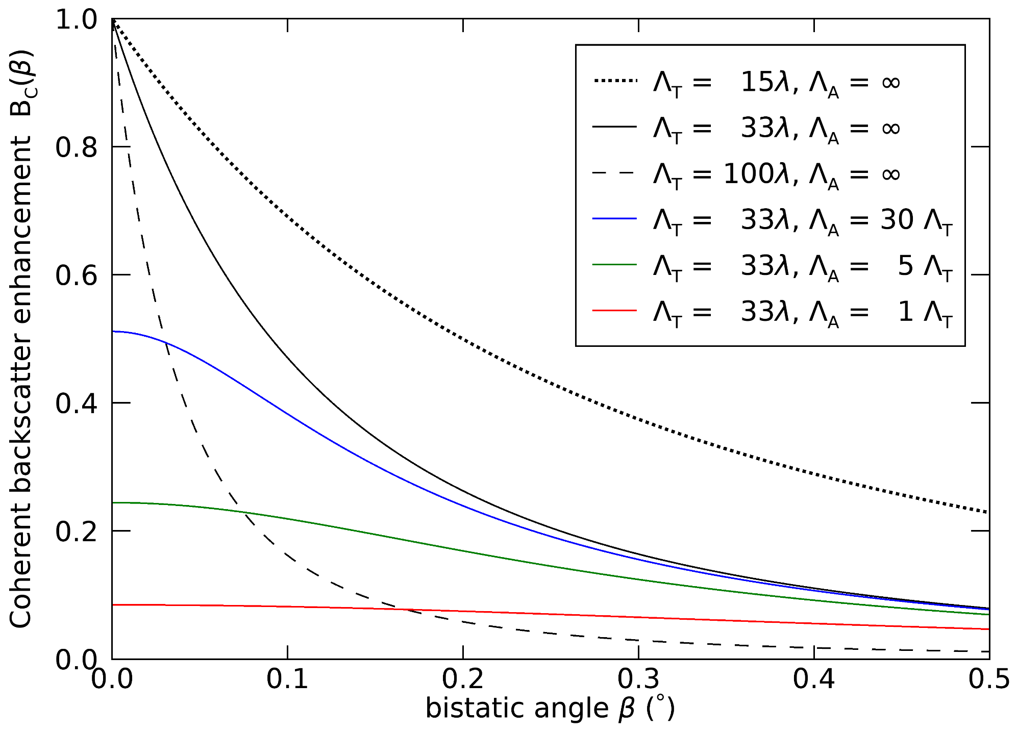
Figure 6Modeled peak shape of the CBOE for different scattering mean free paths ΛT given in multiples of the wavelength λ and for different absorption mean free paths ΛA (in multiples of ΛT) in a medium with small scattering particles (porosity coefficient K=1). For a non-absorbing medium (ΛA=∞) a very sharp peak can be observed. Already with a weak absorption ΛA=30ΛT (blue) the peak height is reduced to 50 % and the peak becomes much rounder. For comparable scattering and absorption lengths the peak is not noticeable (red).
The peak shape, as drawn in Fig. 6, is determined by the ratio of the scattering mean free path ΛT to the wavelength λ, as already indicated by Tsang and Ishimaru (1984), and by the probability distribution of scattering path lengths in the medium. A (monostatic) scattering path begins at the first scattering event in the medium, travels along multiple scatter events with a mean distance ΛT, and ends when the radiation is scattered back out of the medium in the direct return direction (Hapke, 2012, chap. 9.3). In the monostatic configuration, radiation traveling along such a path interferes constructively with radiation propagating along the time-reversed counterpart, thus causing the backscatter intensity enhancement. Long scattering paths, consisting of multiple scattering events, have a longer distance between the path's start and end point and cause a narrow peak, while short scattering paths cause a broad peak. The final peak shape is determined by the sum of all occurring peak shapes of different widths (Tsang and Ishimaru, 1985), weighted according to their occurrence probabilities. An increase in absorption causes shortening of the scattering paths that can contribute to the coherent peak and reduction of the occurrence probability of higher-order scattering; hence the peak becomes rounder and wider (Akkermans et al., 1988, their Fig. 7, and Wolf et al., 1988). Long scattering paths can also be limited by a finite sample (snowpack) thickness, which also causes a rounding of the peak and an increase in its width (Van Der Mark et al., 1988, their Fig. 20, and Van Albada et al., 1988).
Figure 6 shows the shape of the CBOE peak for a range of values of ΛT and ΛA given in multiples of λ. For non-absorbing media (ΛA=∞, black curves), longer scattering lengths ΛT cause a narrower peak with a HWHM of (Van Der Mark et al., 1988; van Albada et al., 1987). This peak width holds for sparsely packed media; for densely packed media of hard spheres, Mishchenko (1992a) suggests a significantly reduced HWHM.
With increasing absorption, the peak height decreases, its width increases, and the peak becomes rounder. To characterize the peak height and width for absorbing media, we found that Eq. (6), with K=1, can be well approximated by
where the factor 1.3 corrects deviation resulting from neglecting first- and second-order terms of ξ(β) in the numerator. Equation (9) provides an analytical form to link the ratio to the peak height:
A slightly more complicated equation can be obtained for the peak width for finite ΛA. Hence, when characterizing the full peak shape or at least its height and width, the parameters ΛT and ΛA can be determined.
Most CBOE models are based on scalar waves which do not consider the vector character of electromagnetic waves, i.e., their polarization. However, experimental and theoretical works show that the CBOE occurs predominantly for co-polarized transmitted and received waves (VV and HH) where the model matches well experimental observation. They also show that the CBOE for cross-polarized (VH) observations is significantly weaker and decreases with increasing sample thickness (van Albada et al., 1987; Mishchenko, 1992b, c; Wolf and Maret, 1985).
2.3.1 Application to KAPRI data
With the two ground-based KAPRI instruments, the benefit of the flexible configuration allows us to sample the intensity peak up to relatively high values of bistatic angle β, and thus the flat region of the intensity curve () should be observable. However, the very top of the peak is difficult to sample due to the non-negligible size of the primary device's antennas, as well as the possibility of the devices obstructing each other's view when placed very close together. Because of this, for analysis of KAPRI data, we use the intensity ratio Ir,∞(β), which is normalized to the incoherent background intensity I(∞) and can be expressed with the aid of Eq. (8) as
To calculate the intensity ratio of Eq. (11) from the actual observed mean ROI intensity , we approximate I(∞) as the mean value of from all acquisitions within the corresponding dataset where β>1∘ (i.e., values well within the flat region of the intensity curve):
Because the model depends on the transport mean free path ΛT and absorption length ΛA through Eqs. (6) and (7), we can use Eq. (11) to fit different values of ΛT and ΛA to the observed intensity curve by nonlinear least-squares minimization. For the fitting procedure, we used the TRF (trust region reflective) optimization method implemented via the curve_fit function of the scipy.optimize library (Virtanen et al., 2020). The initial parameter values of the (ΛT,ΛA) pair were set to (1 m, 100 m), and both parameters were restricted to the non-negative real-number domain.
2.3.2 Application to TanDEM-X data
With TanDEM-X we measured the intensity ratio between the bistatic receiver and the monostatic receiver (Sect. 2.2.2). This approximation is well justified considering that the expected width of the peak is at least 1 order of magnitude larger than the small bistatic angle of the monostatic receiver (see Fig. 6) and that rounding of the peak tip due to weak absorption can be expected. The TanDEM-X measurement can, therefore, be described by Eq. (8) as
The intensity ratio Ir,0(β) is 1.0 for β=0 and reaches its minimum of 0.5 at β→∞ when absorption is negligible. With increasing absorption the ratio lowers and increases from 0.5 to eventually 1.0 when the CBOE is negligible.
A lower limit for the enhancement BC(β=0) can be quickly estimated: because , it follows from Eq. (13) that
i.e., the enhancement BC is at least as large as the relative difference between the monostatic and the bistatic backscatter, and , at the largest available bistatic angle βmax.
To fit the model, we used winter data from the accumulation area (Sect. 2.2.1).
To determine the optimal value of the parameter pair (ΛT,ΛA) and the 95 % confidence intervals, we used the TRF method (Sect. 2.3.1) and set the starting parameter of (ΛT,ΛA) to (2 m, 20 m). However, a sampling of the RMSE in the parameter space of ΛT,ΛA around the optimal value revealed that the global minimum is weakly constrained, and solutions across a large span of values of ΛA provide an acceptably low RMSE value. Thus, to explore multiple parameter pair values, we sampled a range of values of ΛA and used a downhill simplex method implemented in the amoeba IDL function (Nelder and Mead, 1965) to determine the corresponding ΛT.
3.1 Ground-based observations – KAPRI
Figure 7 shows the observed intensity ratio defined by Eq. (12) at HH and VV polarization and the least-squares best fit of the model defined by Eqs. (6), (7), and (11).
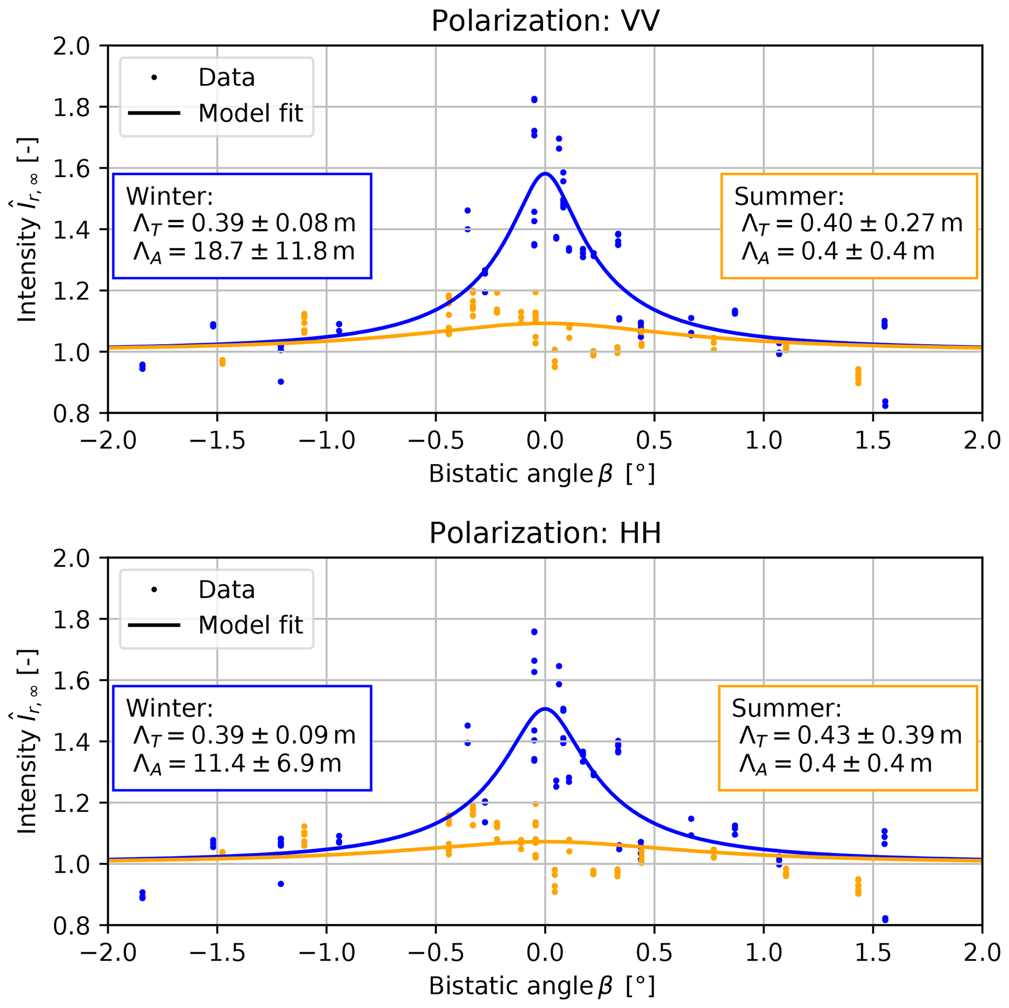
Figure 7Intensity ratio observed during the ground-based experiment (KAPRI), showing backscatter enhancement in the winter dataset (blue). For the summer dataset (orange), the comparable values of the ΛT and ΛA estimates, as well as their relatively large confidence intervals, indicate that the CBOE peak was not detectable. The observed intensities were averaged over the whole region of interest for both polarizations, VV and HH. The blue and orange lines describe the least-squares fit model defined by Eqs. (6), (7), and (11) for winter and summer respectively. The colored boxes for each dataset show the best-fit value and the 95 % confidence interval for the model parameters ΛT and ΛA describing the scattering and absorption mean free paths.

Figure 8Contour plot of root mean square error (RMSE) between measured and modeled winter data in the Ku-band (Fig. 7) for different parameter pairs of ΛA and ΛT. The plot indicates a clear global minimum because the CBOE peak height and hence ΛA can be well estimated due to the availability of ground-based KAPRI measurements at large bistatic angles of β>1∘.
For the winter dataset a clear intensity peak is detected, with a HWHM of approx. 0.25∘ and amplitude BC(0)≈0.5 (1.8 dB), corresponding to m for the HH and VV polarization. The derived absorption lengths ΛA are much longer than the scattering lengths with m for the HH polarization and m for the VV polarization. For the summer dataset, the flat profile of the observed intensity curve indicates that very little or no backscatter enhancement is present – this is reflected in the model fit in the low value and large confidence interval (relative to the value) of the absorption length m. The estimates of the scattering length in the summer dataset ( m and m for the VV and HH polarization respectively) have comparable value to the winter estimates; however the much larger confidence intervals indicate that the value of ΛT could not be determined more precisely for the summer dataset due to the absence of a clear enhancement peak. The uncertainty in the value estimates corresponds to the 95 % confidence interval.
Figure 8 shows the RMSE of the model fit to the dataset with VV polarization, depending on values of the fit parameters ΛT and ΛA. A clear global minimum can be found in the 2-dimensional parameter space at the best-fit parameter values mentioned above, with RMSE of approximately 0.11. Residuals of the model fits for selected values of parameters ΛT and ΛA are shown in Fig. S1.
3.2 Satellite observations – TanDEM-X
3.2.1 Jungfrau–Aletsch region
The large number and wide coverage of the TanDEM-X scenes allow an analysis of the dependency of on β for different land cover types. In Fig. 9, where the color of data points refers to Imono (Fig. 10) to distinguish between dry and wet snow, only in the accumulation area >3500 m (Fig. 9a, b) shows a significant dependence on β: the ratio forms a clear peak that shows some rounding between β=0 and 0.05∘, characteristic of weak absorption. At both polarizations, VV and HH, and only in dry-snow conditions, at the largest available bistatic angles the bistatic backscatter intensity is reduced by approximately 20 % compared to . For wet snow (dark dots) no reduction in is observed at βmax. In contrast, neither the ablation area of the Great Aletsch Glacier, Fig. 9c, nor areas covered by conifer forest, Fig. 9d, show any significant dependence of on β.
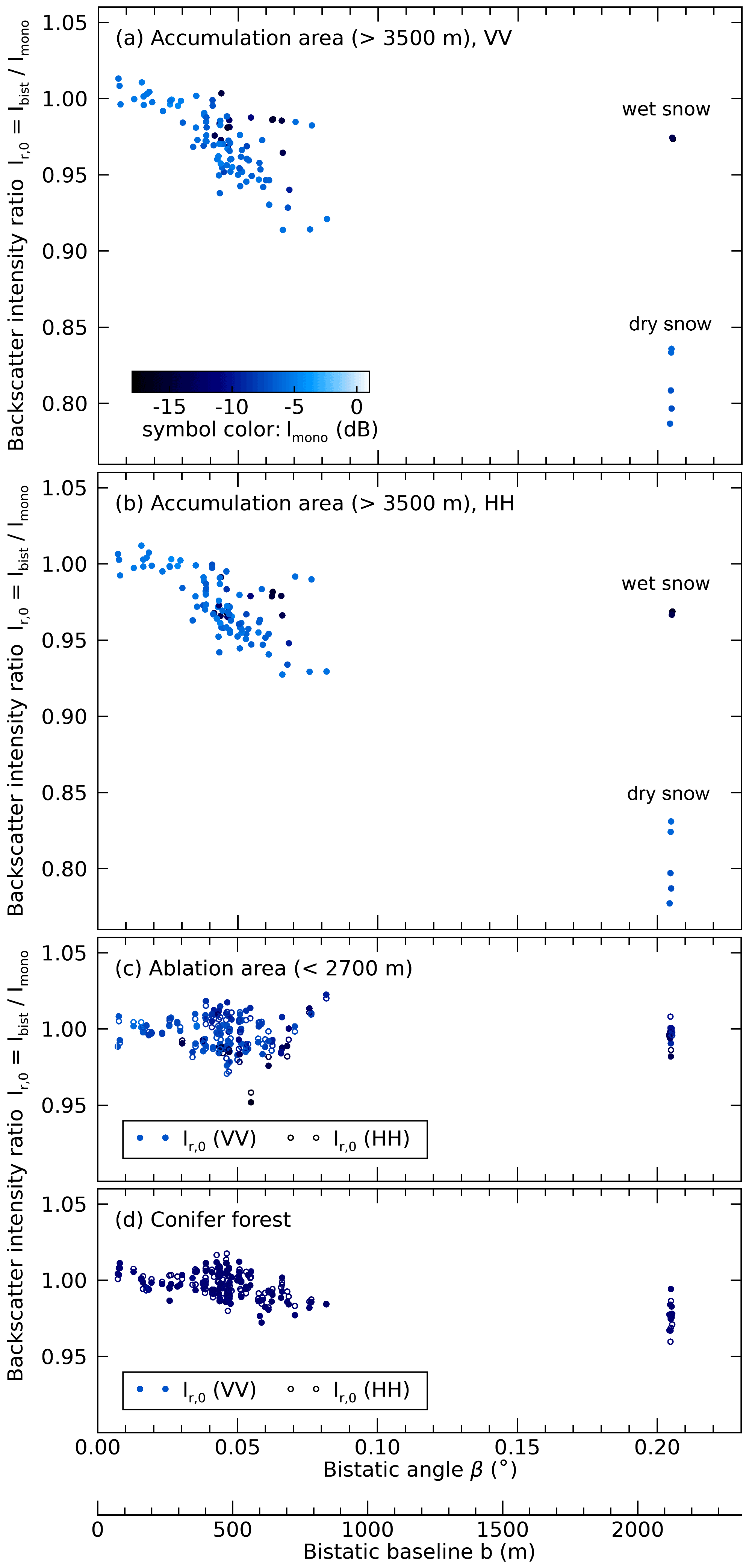
Figure 9(a, b) The intensity ratio observed by the satellite TanDEM-X in the accumulation area. Backscatter enhancement is indicated by the significant dependence of on the bistatic angle β for dry-snow observations at both polarizations (VV, HH). The symbol color indicates the monostatically measured radar brightness Imono and helps to differentiate between wet snow (dark blue) and dry snow (light blue); see Fig. 10a. (c) The ablation area of the Great Aletsch Glacier, located below 2700 m, is covered by 0–3 m of snow in winter but does not show any dependence of on β. (d) Areas covered by conifer forest show no significant dependence on β.
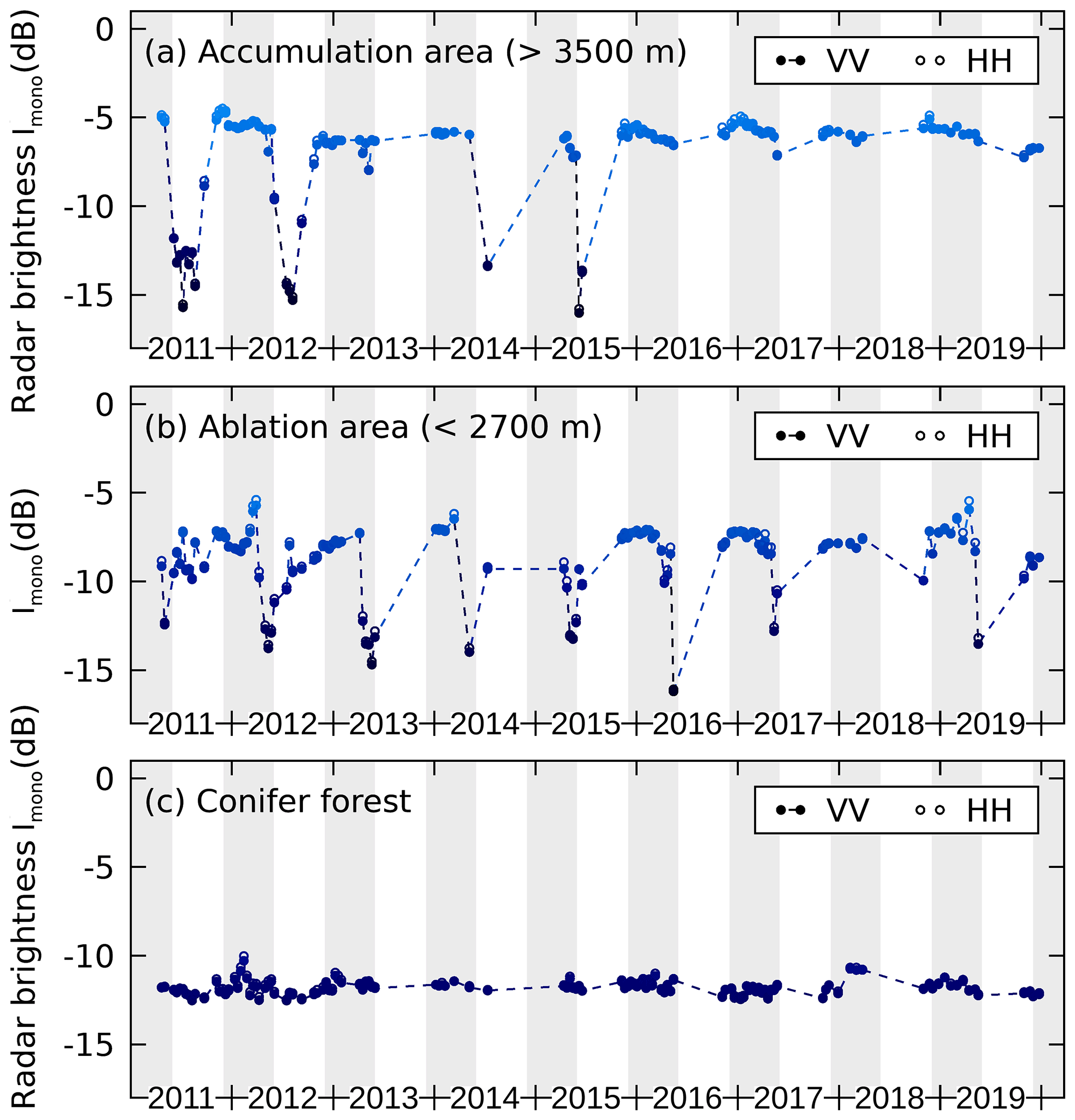
Figure 10Time series of the monostatically measured radar brightness observed by the satellite TanDEM-X for three different land cover types: (a) deep firn in accumulation areas above 3500 m and (b) the tongue of the Great Aletsch Glacier which is covered by 0–3 m of snow in winter. In (a) and (b) seasonal variations in Imono provide a good indicator for distinguishing between dry and wet snow. Gray shading indicates the period 1 December–31 May when dry firn is most likely present in the accumulation zone. This period was selected for estimation of the absorption and scattering lengths ΛA and ΛT. A backscatter difference between the VV and HH polarized data is hardly visible. (c) Compared to snow, forest (mainly conifer forest) shows only small variations in the radar brightness when summer and winter acquisitions are available (2011–2013).
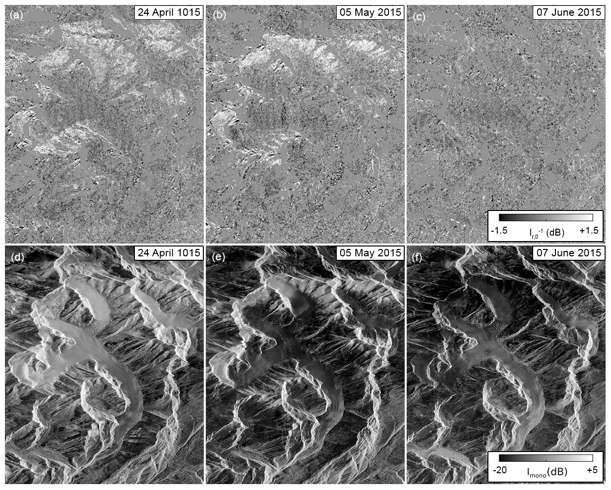
Figure 11(a–c) Monostatic-to-bistatic backscatter ratio , observed by TanDEM-X at the largest available bistatic angles βmax=0.2∘ before (a) and during (b, c) snowmelt. (d–f) Radar brightness for the same dates (d: before snowmelt; e, f: during snowmelt). Areas covered by wet snow appear dark. The Great Aletsch Glacier flows clockwise from top to bottom. In (a) and (b), high-altitude areas (above 3000 and above 3400 m) show backscatter enhancement. In (c) wet snow is present in the entire scene and absorption prevents the CBOE. In (f) an increase in the backscatter intensity becomes visible on the tongue of the Great Aletsch Glacier and on nearby vegetation-covered slopes, indicating that in these areas all snow has melted. Images are shown in slant-range and azimuth coordinates.
To investigate the spatial distribution of areas that show enhanced backscattering, Fig. 11 shows imagery of the monostatic-to-bistatic backscatter ratio together with the radar brightness Imono for a series of three acquisitions with β=βmax at the onset of snowmelt in April and May 2015: on 24 April (Fig. 11a, d), backscatter enhancement is visible for a considerable amount of the area, corresponding to glaciers at high altitude (>3000 m). On 5 May (Fig. 11b, e), the backscatter enhancement is limited to high altitudes because snowmelt is occurring up to an altitude of approximately 3300 m. On 7 June (Fig. 11c, f), snowmelt reaches the peaks of the highest mountains (4274 m) and no enhanced backscattering is detectable at any place.
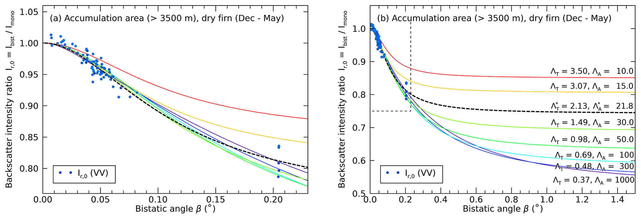
Figure 12(a) Backscatter ratios (dots) restricted to dry firn observations in winter (1 December–31 May; dB) in the accumulation areas of the Jungfrau–Aletsch region from TanDEM-X at VV polarization. Colored lines indicate different CBOE model curves, Eq. (13), parametrized by a range of scattering and absorption parameter combinations (ΛT, ΛA) that can describe the data to different degrees. (b) Same as (a) (in dashed box) but zoomed out to visualize at which β values the different model fits converge to the flat region of the intensity curve where coherent backscatter enhancement is negligible. Measurements at larger bistatic angles of β>0.5∘ could substantially better constrain the total peak height (and thereby ΛA), but such large angles are currently not available.
To estimate the scattering and absorption parameters ΛT and ΛA, as well as the peak width and the backscatter enhancement, we fitted the model, Eq. (13), to the dry firn data of the accumulation area, constrained to winter acquisitions (the selection is specified in Sect. 2.3.2 and indicated by gray shading in Fig. 10a). Figure 12a and b show the selected dataset at two different scales of β. The solution with the minimal RMSE value is indicated by the dashed black line. This solution corresponds to m and m (95 % confidence interval, VV polarization), an enhancement of BC=35 % (+1.3 dB), and a HWHM of the peak of 0.12∘. From the HH polarized data (not shown), we obtained m and m, corresponding to BC=41 % (+1.5 dB) and a HWHM of 0.14∘.
Figure 12a also illustrates that the available data, sampled with a limited range of bistatic angles, allow multiple model solutions with similar RMSE values (colored lines). The solutions are parametrized by different pairs of scattering and absorption mean free paths ΛT and ΛA and were determined by finding ΛT for a fixed ΛA. Table 1 summarizes these parameter pairs and lists for each solution the modeled peak characteristics and the RMSE with respect to the measured data.
Figure 12b illustrates how the different model solutions asymptotically reach the incoherent background at large bistatic angles. The sampling of larger bistatic angles would reveal whether significantly lower values of Ir,0(β) than those observed exist and would, therefore, allow a better constraint on the model parameters.
Table 1Scattering length ΛT, peak height BC(0), and peak width (HWHM) for a set of chosen absorption lengths ΛA determined from the TanDEM-X dataset (VV) of dry firn in the high-altitude accumulation area. The bold-formatted rows indicate the optimal parameter pair at VV and HH polarization. RMSE is the root mean square error between the measured and the modeled value of Ir,0.
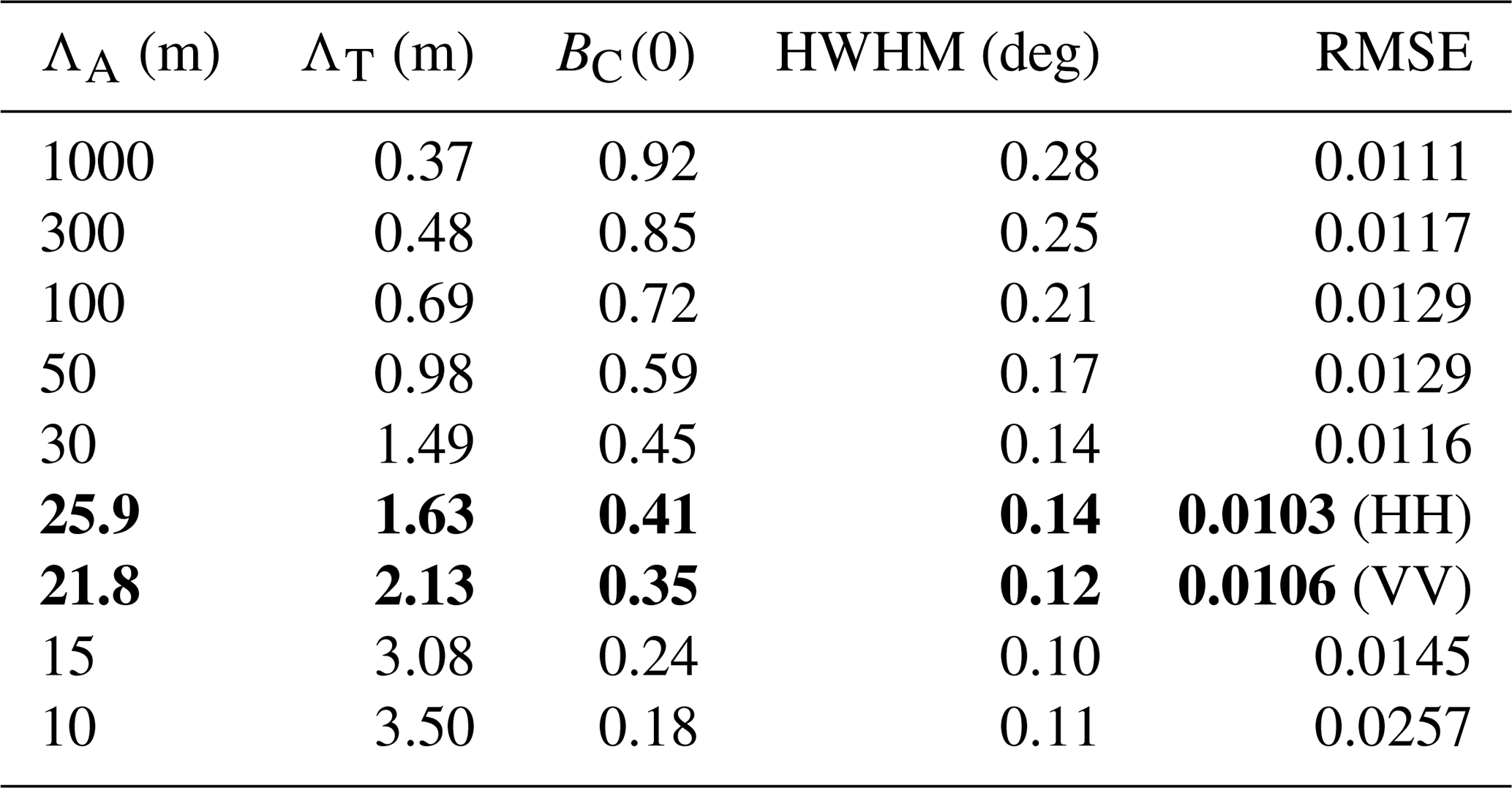
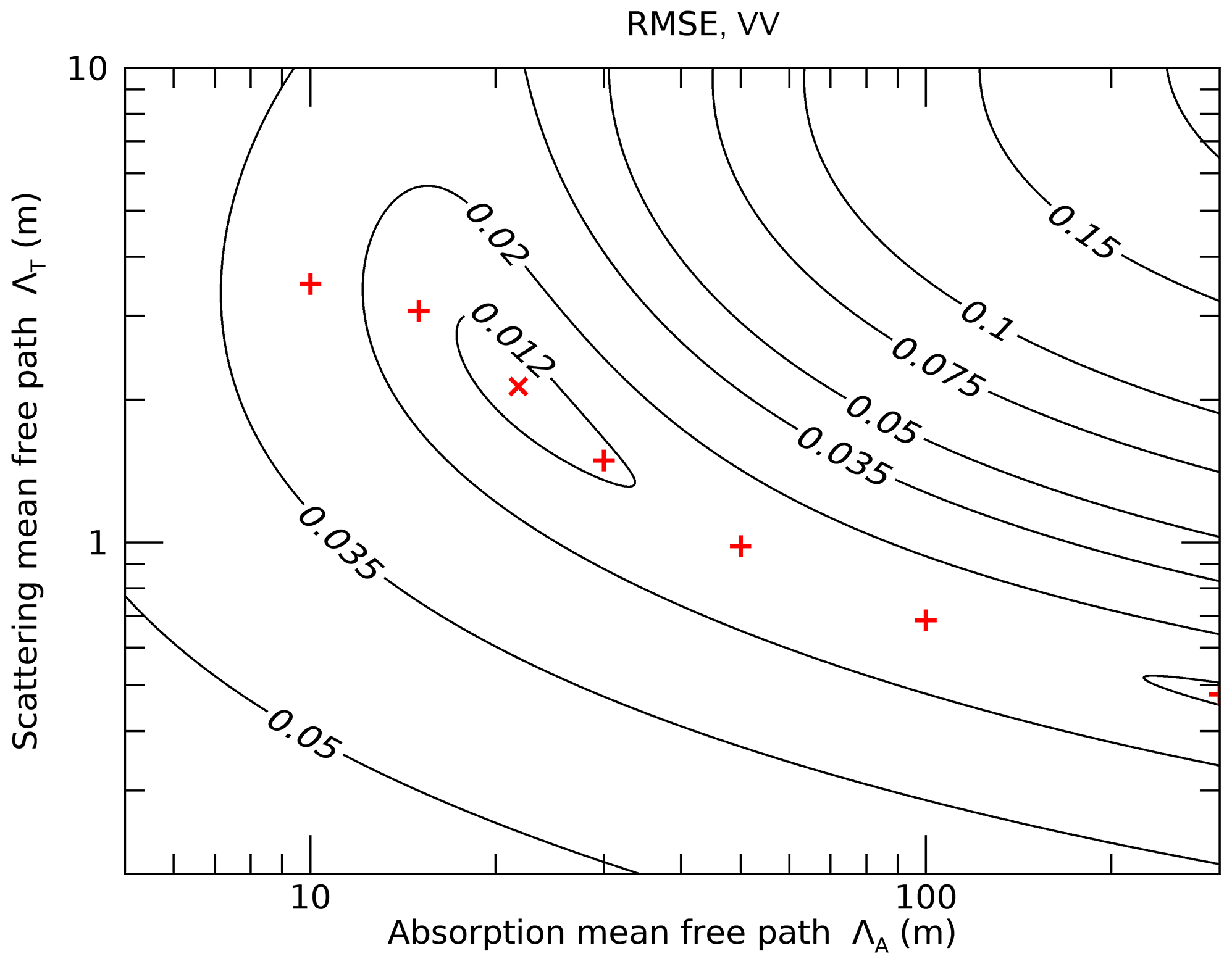
Figure 13Contour map of root mean square error (RMSE) between measured and modeled data for TanDEM-X (Fig. 12) for different pairs of ΛA and ΛT. The plot shows a weak global minimum because acquisitions at sufficiently large β values that could better constrain ΛA were not currently available. The model parameters and RMSE values for the red “+” symbols are given in Table 1. For these points, the parameter value of ΛT was estimated by nonlinear least-squares minimization for different choices of ΛA.
A contour map of the RMSE between the measured and the modeled values (VV) is shown in Fig. 13. While the shallow global minimum (RMSE = 0.0106) is located at the optimal solution ΛT=2.13 m and ΛA=21.8 m, multiple other solutions exist that show only slightly higher RMSE values between 0.011 and 0.015 (see also Table 1). This set of possible parameter pairs (ΛA,ΛT) forms a nonlinear curve (1-dimensional manifold) in the 2-dimensional parameter space (red “+” symbols in Fig. 13).
4.1 Cause of enhancement – CBOE vs. SHOE
In both Ku-band and X-band observations of terrestrial snow, we observed narrow intensity peaks with an angular width of a fraction of 1∘. These peaks are clearly attributable to the CBOE as opposed to the SHOE, which follows from a comparison of the effects' properties as described by Hapke (2012, chap. 9).
Firstly, the SHOE requires that the scatterers are much larger than the wavelength of the incident radiation so that they can cast sharp shadows. This requirement can hardly be fulfilled at radar wavelengths of several centimeters since ice particles in snow have average diameters on the order of millimeters (Kuga et al., 1991). A grain size of 0.3–1.5 mm was observed in the seasonal snowpack studied by the KAPRI experiment (Fig. 2). The snowpack did not show any centimeter-sized ice structures that could have been caused by strong melt events. Furthermore, the narrow peak width is in agreement with characteristics of the CBOE, while a SHOE peak usually has a width of several degrees or tens of degrees, depending on particle size distribution. Finally, the SHOE is only present in media where single scattering is dominant. Multiple-scattering processes decrease the amplitude of the SHOE and increase the amplitude of the CBOE. Since dry snow is a weakly absorbing medium for microwaves where multiple (i.e., volume) scattering is considerable (Kuga et al., 1991), the CBOE is expected to be the dominant effect.
4.2 Observations of CBOE
4.2.1 Ground-based observations – KAPRI
Figure 7 shows a statistically significant enhancement peak for the winter acquisition and a lack of such a peak for the summer dataset, which was acquired using an identical target region of interest, identical acquisition procedure (except platform substitution to allow movement on snow/the road), and identical processing pipeline. The summer dataset thus serves as a useful control which ensures that the detected enhancement peak is not an erroneous artifact of the bistatic data processing pipeline, and it also indicates that the enhancement peak is indeed caused by the snow layer present on the hillside. In the summer scenario (i.e., absence of a clear backscatter enhancement peak), the model, described in Sect. 2.3 and visualized in Fig. 6, predicts that the absorption length is shorter than or equal to the scattering length (ΛA≤ΛT). An interpretation of this scenario is that higher-order scattering paths are suppressed due to absorption, and thus the summer scenario is dominated by a single-scattering process. In the summer scenario the model becomes much less sensitive to the precise value of ΛT (which is a measure of the width of the peak), and thus estimates of this value have much higher uncertainty as opposed to the case of a clearly detectable enhancement peak in winter.
The best-fit values of model parameters in Fig. 7 indicate a scattering mean free path value ΛT between 30 and 50 cm and an absorption length ΛA between 6 and 24 m at both polarizations, which matches well the observations by Wiesmann et al. (1998). No statistically significant difference in the parameter estimates is observed between the HH and VV polarized data. This is well aligned with the theoretical model of Mishchenko (1992b), in which there is only a very small difference between the co-polarized backscatter enhancement factors at these two polarizations. The HWHM of the angular peak of ≈0.25∘ is sufficiently wide so that KAPRI's transmit antennas' non-zero size, which limits the angular resolution to 0.05∘ (Sect. 2.1.2), has only a very limited effect on the precision with which the width and height of the peak can be determined.
The snow depth during the winter acquisitions was measured on-site as approximately 1.5 m (Fig. 2), and thus the estimate of ΛA is several times higher than the snow depth. The extremely shallow local incidence angle (above 70∘ for the vast majority of the ROI area) and short transport mean free path ΛT would likely lead to longer trajectories of the radiation through the snow medium before reaching the ground. Nevertheless, the optical thickness of the snow depth d of only three to four scattering mean free paths ΛT could limit higher-order scattering. While Tsang and Ishimaru (1985) conclude that already at τd=4, models approximate well the half-space solution (where τd=∞), Van Der Mark et al. (1988) (Figs. 9, 12) show that the peak height and width, at least for very weakly absorbing media (ΛA≫ΛT), might be affected up to τd≈30. Missing higher-order scattering, in turn, is an explanation for a rounding of the peak shape (Akkermans et al., 1988, Fig. 7). During the field experiment, a corner reflector lowered to the bottom of a 1.55 m deep snow pit with vertical walls was still visible, indicating that at least a fraction of microwaves reached the ground, thereby limiting higher-order scattering.
4.2.2 Satellite observations – TanDEM-X
A significant dependence of the backscatter intensity on the bistatic angle, , is only visible in the accumulation zones of the Jungfrau–Aletsch region with altitude H>3500 m (Fig. 9a, b). Above this altitude, a firn layer with below-freezing snow temperatures is present to a depth of several tens of meters (Haeberli and Alean, 1985; Suter et al., 2001). This thick and cold firn layer represents a disordered medium where multiple scattering is possible and at the same time microwave absorption is weak because liquid water is absent. The existence of the CBOE in dry firn is further supported by the spatial and temporal distribution of an enhanced brightness ratio . Spatially, the enhancement matches the accumulation area of high-altitude glaciers in the Jungfrau–Aletsch region (Fig. 11). Temporally, the backscatter enhancement vanishes in these areas when snowmelt sets in, and thus the scattering predominantly takes place at the snow surface. These observations were confirmed by additional data from the Teram Shehr and Rimo glaciers in the Karakorum (see Supplement).
The rounding of the peak shape in Fig. 12a indicates that either absorption or a limited thickness of firn is present in the accumulation area. Field measurements indicate cold firn in at least the upper 8 m (Jacqueline Bannwart, personal communication, 2021), and literature data indicate that temperate firn might be present at around 15 m below the surface (Suter et al., 2001). The global minimum at ΛT=2.1 m and ΛA=21.8 m in Fig. 13 might therefore provide a realistic estimate for ΛA as larger absorption lengths are difficult to conform to field measurements. Our observed values for absorption and scattering lengths also agree with the measurements by Wiesmann et al. (1998).
On the tongue of the Great Aletsch Glacier, where a seasonal snowpack is present during winter, no backscatter enhancement was observed in the X-band (Fig. 9c). As seasonal snow is younger than multi-year firn, smaller snow grain sizes are expected, resulting in scattering lengths larger than the value ΛT=2.1 m determined for the accumulation area. The thickness of the seasonal snowpack of 0–3 m corresponds therefore to an optical thickness of τd≈1 or less, which considerably affects the peak intensity (Van Der Mark et al., 1988, Fig. 9). In consequence, the single scattering at the (possibly rough) snow–ice interface at the bottom of the snowpack can remain the dominant scattering process. The low average number of scattering events in the seasonal snow volume is, therefore, not sufficient for the CBOE to occur on the ablation area of the Great Aletsch Glacier.
In forest-covered areas, no significant dependency of on β is visible. We think the reason for this is that, compared to dry snow, multiple scattering at the X-band is reduced in forest due to absorption of microwaves; hence the CBOE is prevented.
We also did not observe coherent backscatter enhancement in any area other than the high-accumulation area, even though the tongue of the Great Aletsch Glacier is highly crevassed and valley slopes are covered by rock debris. From this we conclude that in the X-band, rough surfaces do not elicit the CBOE.
4.2.3 Comparison of bistatic measurement geometries
The KAPRI experiment sampled a larger range of bistatic angles (up to 1.92∘) so that the flat incoherent intensity background I0 could be sampled. Therefore, both the width and the height of the enhancement peak in winter can be constrained much better than with the TanDEM-X observations where . This, in turn, translates to better-constrained estimates of parameters ΛT and ΛA as illustrated by the clearly visible global minimum in the plot of the RMSE value in Fig. 8 as compared to Fig. 13.
Compared to the KAPRI experiment, the bistatic angles sampled by TanDEM-X are relatively small, making it possible that not the entire peak of the CBOE was sampled. In consequence, the bistatic data at βmax=0.2∘ might still be affected by the CBOE. Missing measurements at larger bistatic angles result in a weak constraint of the parameter pair (ΛT, ΛA), permitting a range of value pairs that each can fit the data (Table 1 and Figs. 12 and 13). To better constrain the observed values of ΛT and ΛA, bistatic angles of at least β=0.5∘ would need to be sampled by TanDEM-X. However, such larger angles are currently not available.
4.3 Impact of the CBOE on backscatter observations
Generally, the existence of a narrow backscatter enhancement peak around the monostatic direction needs to be kept in mind when performing backscatter measurements of snow, regardless of whether the sensors used are considered monostatic or bistatic. On one hand, for truly monostatic sensors the CBOE is strongest. On the other hand, some radar sensors are considered monostatic even though they have a small but non-zero spatial separation between the transmitting and receiving antennas. Due to this bistatic baseline, the detected backscatter intensity value could be significantly reduced compared to the value that would have been detected by a truly monostatic sensor. When prior estimates of ΛT and ΛA over a particular medium are available, Eq. (6) could be used to roughly estimate the width and height of the peak, which can subsequently be used to estimate bistatic angle values where the CBOE might affect the measurements (see also Sect. 4.4).
As an example of the necessity to precisely align the measurement geometry to the expected width of the peak, Tan et al. (2015) compared modeled results to active and passive microwave measurements at the X- to Ka-band performed in Sodankylä, Finland, as part of the NoSREx field experiment (Lemmetyinen et al., 2016). The active measurements were performed with the SnowScat instrument (Wiesmann et al., 2010). The model, which includes backscatter enhancement into the dense-media radiative transfer (DMRT) theory, might provide a significant step forwards for modeling of the radar backscatter signal from snow. However, if the peak width of the CBOE in the NoSREx experiment were comparable to the narrow observed peak widths in our study (∘), the bistatic angles of the SnowScat measurements would actually be 1 order of magnitude too large to observe the CBOE. This follows from the instrument height of 9.6 m, the incidence angle range of 30–60∘ (Lemmetyinen et al., 2016), and the antenna separation of 72 cm (Wiesmann et al., 2010; Wiesmann and Werner, 2010), resulting in bistatic angle values of β=1.8 to .
Except for possible extreme cases of a medium causing an extremely narrow enhancement peak (with width on the order of thousandths of a degree), the velocity-induced bistatic angle βv of moving radar platforms is negligible in the context of the CBOE. For the side-looking geometry, the bistatic angle βv caused by platform motion with velocity v can be calculated as , where c is the speed of light. Thus, for all conventional sensors – even for satellite platforms in low Earth orbit moving at speeds of 6–8 km h−1 – the resulting value of βv is on the order of thousandths of a degree or less.
4.4 Link to the microstructure of snow
In the model outlined in Sect. 2.3, which assumes an optically thick medium, the two parameters ΛT and ΛA, defining the peak shape, can be linked to the snow microstructure and to the density of snow. The transport mean free path ΛT≥ΛS is a measure of the medium's scattering properties and corresponds to the scattering mean free path for particles that scatter EM radiation symmetrically in the forward and backward direction (Hapke, 2012, Eq. 7.24b and Sect. 5.2.7); see also Van Der Mark et al. (1988, Sect. IV-A). For negligible absorption, ΛT describes the one-way penetration depth where the incident radiation is reduced to by sideways scattering. While in the context of CBOE modeling, the (volume-averaged) scattering coefficient S is derived from the scattering cross-section of individual particles in sparse media (Hapke, 2012, chap. 5; Ishimaru, 1978, chap. 2; and Van Der Mark et al., 1988), for snow the scattering coefficient needs to be estimated with dense-media radiative transfer theories like DMRT (e.g., Tsang et al., 2007) or the improved Born approximation (IBA) (Mätzler, 1998) as shown in Picard et al. (2018, Sect. 3.1) and as already indicated by Mishchenko (1992a). The description of the SMRT model (Picard et al., 2018) provides a direct relation between the scattering coefficient S and the phase function and links these to the autocorrelation function of the medium indicator function that represents the spatial 3D microstructure of the snow–ice matrix (Löwe and Picard, 2015). Still, both theories, DMRT and IBA, are not yet sufficiently parametrized by field-measurable quantities (Picard et al., 2018). An empirical relation to link the microstructure to S is given in Wiesmann and Mätzler (1999).
The absorption mean free path is a measure of the medium's absorbing properties given by the volume-averaged absorption coefficient A (Hapke, 2012, Eq. 7.18a). For negligible scattering, ΛA describes the absorption length where the incident radiation intensity is reduced to ; for continuous media (without scatterers) A would be equivalent to the absorption coefficient with ni being the imaginary part of the refractive index. For snow, Picard et al. (2018) recommend computation of ni from the Polder–van Santen formula, e.g., in Sihvola (2000), Mätzler (1998), and Wiesmann and Mätzler (1999); the refractive index of pure ice is given by Warren and Brandt (2008).
The absorption and scattering coefficient sum to the extinction coefficient , which corresponds in the sparse-media models from Tsang and Ishimaru (1984, 1985) and Van Der Mark et al. (1988, below Eq. 26b) by to the effective propagation constant K′′ that is related to particle absorption and scattering properties described by the scattering amplitude f.
4.5 Limitations of the model
The CBOE model used in this work can accurately predict the peak shapes observed in various volume fractions of colloidal suspensions where the particle sizes are within the order of magnitude of the wavelength (Van Der Mark et al., 1988; Akkermans et al., 1988). The parameters of the model, in particular the scattering coefficient and absorption coefficient that determine the shape of the CBOE peak, can, in theory, be estimated from the microstructure and density of the snowpack when considering dense-media scattering theories (Picard et al., 2018); see also Mishchenko (1992a), who addresses a snow-like structure. However, the often complex (multi-layer) snow structure (e.g., Proksch et al., 2015) together with current limitations in accurately predicting the scattering coefficients from the snow microstructure (Vargel et al., 2020) might prevent a precise estimate of the peak shape even though a rough estimate of the peak width is feasible. An additional limitation for an accurate estimation of ΛA, as well as possibly ΛT, results from the assumption that the scattering medium fills a semi-infinite space, whereas the snowpack has a limited optical thickness τd. Hence, ΛA might be underestimated due to limited layer thickness (Van Der Mark et al., 1988; Van Albada et al., 1988).
Our observations of the CBOE peak shape originate from natural (non-homogeneous) snow cover, and currently no laboratory experiments of the CBOE at microwave frequencies, including a precise characterization of the microstructure, are available. Such experiments could validate the model used and might indicate whether adaption of the model or introduction of additional correction factors could be required in order to precisely link the microstructure to the CBOE peak shape. Nevertheless, we clearly observed the CBOE peak in natural snow, which can lead to development of new methods for snow and ice monitoring.
4.6 Applications based on the CBOE
In TanDEM-X data we have observed a backscatter enhancement of at least 1.3 dB for firn-covered areas of the European Alps and in the Karakorum, while for firn-free areas no backscatter enhancement could be observed. This suggests that detection of deep firn with the X-band is possible when large enough bistatic angles, β>0.2∘, are available.
For seasonal snow, we observed a clear CBOE peak (∼1.8 dB of backscatter enhancement) at the Ku-band using KAPRI, whereas in the X-band we were not able to observe an enhancement. The higher sensitivity of high-frequency systems (Ku- or possibly Ka-band) for detecting the CBOE in seasonal snow results from the shorter scattering length since sufficiently high-order scattering events can occur within the snow layer of limited thickness. Furthermore, the difference between KAPRI observations in summer (no CBOE from vegetation) and winter (snow-induced CBOE) demonstrates how Ku-band bistatic observations could potentially provide a means to discriminate dry snow from vegetation and therefore provide a means to map snow cover extent. Beyond that, the frequency dependency of the scattering lengths makes a characterization of the intensity of the CBOE at multiple frequencies possible, which, in turn, could allow a quantitative characterization of the height or water equivalent of seasonal snow. The area covered by snow, the snow depth, and the snow water equivalent are considered key data products for the snow essential climate variable (Belward et al., 2016). Bistatic missions characterizing the CBOE occurring in snow can thus be an asset in mapping these data products.
In terms of polarimetric measurements, the results of this study, as well as experimental work and theoretical models (van Albada et al., 1987; Mishchenko, 1992b, c; Wolf and Maret, 1985), indicate that the effect is present predominantly in co-polarized channels and the effect is equally strong at both horizontal and vertical polarizations. Nevertheless, in further studies the use of full-polarimetric radar systems can still be advantageous, e.g., to decisively differentiate the CBOE and the SHOE based on their different impact on linear and circular polarization ratios (Rignot, 1995; Hapke, 2012, Sect. 9.4).
Existing bistatic ground-based SAR sensors (Pieraccini and Miccinesi, 2017; Wang et al., 2019) and to a certain extent also airborne bistatic SAR sensors (Dubois-Fernandez et al., 2006; Meta et al., 2018) could be employed to study the effect locally with a high temporal resolution and to observe temporal variations in the effect as well as its dependence on layer thickness and snow structure. Spaceborne platforms, while limited by orbital mechanics and repeat intervals, can provide a means to sample and to characterize the CBOE on the global scale. Finally, our characterization of the CBOE at the X- and Ku-band in terrestrial snow could inspire future inter-planetary missions aiming to search for water ice and possibly other types of snow to employ bistatic radar measurements.
In this work we presented the first observations of the coherent backscatter opposition effect (CBOE) and the sampling of its angular peak shape at radio wavelengths within the Earth's cryosphere. The existence of the peak was confirmed in seasonal dry snow cover at Ku-band wavelengths by the ground-based bistatic radar system KAPRI. With the bistatic satellite formation TanDEM-X, the effect was also confirmed at the X-band within the accumulation zone of high-altitude glaciers in the European Alps and the Karakorum.
The observability of the CBOE in bistatic radar measurements of snow presents an opportunity for future satellite missions aiming to derive snow properties from synthetic-aperture radar data on the global scale. The radiometric precision requirement for such a spaceborne radar system is demanding since the theoretical maximal amplitude of the effect is 3 dB – in this study, we were able to characterize the peak using TanDEM-X and data-driven radiometric calibration. Deployment of such bistatic systems – at bistatic angles up to 1 or 2∘ and covering the entire CBOE peak including the incoherent background – would open up a new pathway to characterize snow through microwave scattering.
The Ku-band observations presented in this paper suggest that the CBOE can be used as an indicator for presence of seasonal snow cover. At the X-band, the CBOE could be applied to detect dry snow thicker than several meters, e.g., multi-year firn in accumulation areas of glaciers. Furthermore, through analysis of the angular width and height of the enhancement peak, scattering and absorption mean free paths within the snowpack can be estimated. Knowledge of the scattering mean free path and the discrimination between single (surface) and higher-order (volume) scattering in areas where the CBOE is present could help to better constrain the radar penetration depth, which, in turn, is crucial for precise surface height estimation by means of radar altimetry and interferometry.
The CBOE thus provides a pathway towards better characterization of areas covered by snow and possibly also snow depth and snow water equivalent, which are the three key data products for snow as an essential climate variable. Furthermore, the detection and characterization of the CBOE in terrestrial snow also are an encouraging sign for applying this measurement concept to space missions which aim to confirm the presence of water ice on surfaces of other solar system bodies.
TanDEM-X data are available from DLR at https://tandemx-science.dlr.de/ (DLR, 2022) and were provided by the proposal leinss_XTI_GLAC6870. KAPRI SLC data, as well as data values for plots, are published in the ETH Research Collection with the DOI https://doi.org/10.3929/ethz-b-000516171 (Stefko, 2021).
The supplement related to this article is available online at: https://doi.org/10.5194/tc-16-2859-2022-supplement.
SL conceptualized the study of coherent backscatter enhancement in snow with bistatic radar. MS and SL designed the Davos field experiment and wrote the manuscript together. MS processed and analyzed the ground-based data and SL the spaceborne data. IH suggested exploration of bistatic radar signals with KAPRI. All authors reviewed, edited, and approved the submitted version of the manuscript.
The contact author has declared that none of the authors has any competing interests.
Publisher’s note: Copernicus Publications remains neutral with regard to jurisdictional claims in published maps and institutional affiliations.
The authors would like to thank Henning Löwe and the anonymous reviewer for their in-depth peer reviews and for constructive comments and suggestions on how to improve the paper. Furthermore, the authors would like to thank Tingting Li, Yuta Izumi, Simone Jola, and Michael Arnold for their support during fieldwork in Davos; Christian Mätzler and Rosemary Willatt for valuable feedback and discussion; Emmanuel Trouvé for proofreading the manuscript; Laurane Charrier for valuable input regarding applications of the CBOE; and Thomas Busche for support with the TanDEM-X acquisitions. The authors would also like to thank Reto Müller for access to his property during acquisitions and the staff of Bergbahnen Rinerhorn AG for assistance with equipment transportation. The TanDEM-X data were provided by the German Aerospace Center (DLR) via proposal XTI_GLAC6780.
Silvan Leinss was supported by the French Ministry for Europe and Foreign Affairs, within the framework of the third “Make Our Planet Great Again” (MOPGA) program (mopga-postdoc-3) for postdoctoral researchers. The MOPGA grant has been issued by Campus France under grant no. 0821369222.
This paper was edited by Carrie Vuyovich and reviewed by Henning Löwe and one anonymous referee.
Aegerter, C. M. and Maret, G.: Coherent Backscattering and Anderson Localization of Light, Prog. Optics, 52, 1–62, https://doi.org/10.1016/S0079-6638(08)00003-6, 2009. a
Akkermans, E. and Montambaux, G.: Mesoscopic physics of photons, J. Opt. Soc. Am. B, 21, 101–112, https://doi.org/10.1364/JOSAB.21.000101, 2004. a
Akkermans, E., Wolf, P. E., and Maynard, R.: Coherent backscattering of light by disordered media: Analysis of the peak line shape, Phys. Rev. Lett., 56, 1471–1474, https://doi.org/10.1103/PhysRevLett.56.1471, 1986. a, b
Akkermans, E., Wolf, P., Maynard, R., and Maret, G.: Theoretical study of the coherent backscattering of light by disordered media, J. Phys. France, 49, 77–98, https://doi.org/10.1051/jphys:0198800490107700, 1988. a, b, c, d, e, f, g
Baffelli, S., Frey, O., Werner, C., and Hajnsek, I.: Polarimetric Calibration of the Ku-Band Advanced Polarimetric Radar Interferometer, IEEE T. Geosci. Remote, 56, 2295–2311, 2017. a
Belward, A., Bourassa, M., Dowell, M., et al.: The global observing system for climate: implementation needs, Tech. Rep., GCOS-200, World Meteorological Organization, https://gcos.wmo.int/en/gcos-implementation-plan (last access: 12 July 2022), 2016. a
Black, G. J., Campbell, D. B., and Nicholson, P. D.: Icy Galilean Satellites: Modeling Radar Reflectivities as a Coherent Backscatter Effect, Icarus, 151, 167–180, https://doi.org/10.1006/icar.2001.6616, 2001. a
DLR: TanDEM-X Science Service System, DLR [data set], https://tandemx-science.dlr.de/, last access: 9 June 2022. a
Dubois-Fernandez, P., Cantalloube, H., Vaizan, B., Krieger, G., Horn, R., Wendler, M., and Giroux, V.: ONERA-DLR bistatic SAR campaign: Planning, data acquisition, and first analysis of bistatic scattering behavior of natural and urban targets, Radar, Sonar and Navigation, IEE P.-Radar Son. Nav., 153, 214–223, https://doi.org/10.1049/ip-rsn:20045117, 2006. a
Duque, S., Balss, U., Rossi, S., Fritz, T., and Balzer, W.: TanDEM-X Payload Ground Segment CoSSC Generation and Interferometric Considerations, TD-PGS-TN-3129, issue 1.0, Remote Sensing Technology Institute, DLR, https://tandemx-science.dlr.de/pdfs/TD-PGS-TN-3129_CoSSCGenerationInterferometricConsiderations_1.0.pdf (last access: 12 July 2022), 2012. a, b
Fierz, C., Armstrong, R. L., Durand, Y., Etchevers, P., Greene, E., McClung, D. M., Nishimura, K., Satyawali, P. K., and Sokratov, S. A.: The International Classification for Seasonal Snow on the Ground, IHP-VII Technical Documents in Hydrology No. 83, IACS Contribution No. 1, UNESCO-IHP, Paris, https://unesdoc.unesco.org/ark:/48223/pf0000186462 (last access: 12 July 2022), 2009. a
Fritz, T., Brautigam, B., Krieger, G., and Zink, M.: TanDEM-X Ground Segment – TanDEM-X Experimental Product Description, TD-GS-PS-3028, issue 1.2, DLR, 1.2 edn., https://tandemx-science.dlr.de/pdfs/TD-GS-PS-3028_TanDEM-X-Experimental-Product-Description_1.2.pdf (last access: 12 July 2022), 2012. a, b
Haeberli, W. and Alean, J.: Temperature and Accumulation of High Altitude Firn in the Alps, Ann. Glaciol., 6, 161–163, https://doi.org/10.3189/1985AoG6-1-161-163, 1985. a
Hajnsek, I., Busche, T., Krieger, G., Zink, M., Schulze, D., and Moreira, A.: Announcement of opportunity: TanDEM-X science phase, Tech. Rep. TD-PD-PL-0032, Microwave and Radar Institute (DLR-HR), https://tandemx-science.dlr.de/pdfs/TD-PD-PL_0032TanDEM-X_Science_Phase.pdf (last access: 12 July 2022), 2014. a
Hapke, B.: Bidirectional reflectance spectroscopy: 4. The extinction coefficient and the opposition effect, Icarus, 67, 264–280, https://doi.org/10.1016/0019-1035(86)90108-9, 1986. a, b
Hapke, B.: Coherent backscatter and the radar characteristics of outer planet satellites, Icarus, 88, 407–417, https://doi.org/10.1016/0019-1035(90)90091-M, 1990. a
Hapke, B.: Theory of Reflectance and Emittance Spectroscopy, 2 edn., Cambridge University Press, ISBN 9781139025683, https://doi.org/10.1017/CBO9781139025683, 2012. a, b, c, d, e, f, g, h, i, j, k, l, m, n, o
Hapke, B., DiMucci, D., Nelson, R., and Smythe, W.: The cause of the hot spot in vegetation canopies and soils: Shadow-hiding versus coherent backscatter, Remote Sens. Environ., 58, 63–68, https://doi.org/10.1016/0034-4257(95)00257-X, 1996. a, b
Hapke, B., Nelson, R., and Smythe, W.: The Opposition Effect of the Moon: Coherent Backscatter and Shadow Hiding, Icarus, 133, 89–97, https://doi.org/10.1006/icar.1998.5907, 1998. a
Hapke, B. W., Nelson, R. M., and Smythe, W. D.: The Opposition Effect of the Moon: The Contribution of Coherent Backscatter, Science, 260, 509–511, https://doi.org/10.1126/science.260.5107.509, 1993. a
Ishimaru, A.: Wave propagation and scattering in random media, 1st edn., vol. 1–2, Academic press New York, ISBN 978-0-12-374701-3, https://doi.org/10.1016/B978-0-12-374701-3.X5001-7, 1978. a
Jun, L., Wang, W., and Zwally, H. J.: Interannual variations of shallow firn temperature at Greenland summit, Ann. Glaciol., 35, 368–370, 2002. a
Kaasalainen, S., Kaasalainen, M., Mielonen, T., Suomalainen, J., Peltoniemi, J. I., and Näränen, J.: Optical properties of snow in backscatter, J. Glaciol., 52, 574–584, https://doi.org/10.3189/172756506781828421, 2006. a
Krieger, G., Moreira, A., Fiedler, H., Hajnsek, I., Werner, M., Younis, M., and Zink, M.: TanDEM-X: A satellite formation for high-resolution SAR interferometry, IEEE T. Geosci. Remote, 45, 3317–3341, 2007. a
Kuga, Y. and Ishimaru, A.: Retroreflectance from a dense distribution of spherical particles, J. Opt. Soc. Am. A, 1, 831–835, https://doi.org/10.1364/josaa.1.000831, 1984. a, b
Kuga, Y., Ulaby, F. T., Haddock, T. F., and DeRoo, R. D.: Millimeter‐wave radar scattering from snow 1. Radiative transfer model, Radio Sci., 26, 329–341, https://doi.org/10.1029/90RS02560, 1991. a, b
Leinss, S. and Bernhard, P.: TanDEM-X:Deriving InSAR Height Changes and Velocity Dynamics of Great Aletsch Glacier, IEEE J. Sel. Top. Appl., 14, 4798–4815, https://doi.org/10.1109/JSTARS.2021.3078084, 2021. a, b, c
Lemmetyinen, J., Kontu, A., Pulliainen, J., Vehviläinen, J., Rautiainen, K., Wiesmann, A., Mätzler, C., Werner, C., Rott, H., Nagler, T., Schneebeli, M., Proksch, M., Schüttemeyer, D., Kern, M., and Davidson, M. W. J.: Nordic Snow Radar Experiment, Geosci. Instrum. Method. Data Syst., 5, 403–415, https://doi.org/10.5194/gi-5-403-2016, 2016. a, b
Löwe, H. and Picard, G.: Microwave scattering coefficient of snow in MEMLS and DMRT-ML revisited: the relevance of sticky hard spheres and tomography-based estimates of stickiness, The Cryosphere, 9, 2101–2117, https://doi.org/10.5194/tc-9-2101-2015, 2015. a
Lucas, C., Leinss, S., Bühler, Y., Marino, A., and Hajnsek, I.: Multipath interferences in ground-based radar data: A case study, Remote Sensing, 9, 1260, https://doi.org/10.3390/rs9121260, 2017. a
Mätzler, C.: Improved Born approximation for scattering of radiation in a granular medium, J. Appl. Phys., 83, 6111–6117, https://doi.org/10.1063/1.367496, 1998. a, b
Mätzler, C. and Wegmüller, U.: Dielectric properties of freshwater ice at microwave frequencies, J. Phys. D: Appl. Phys., 20, 1623–1630, https://doi.org/10.1088/0022-3727/20/12/013, 1987. a
Mätzler, C. and Wegmüller, U.: Dielectric properties of freshwater ice at microwave frequencies – Errata, J. Phys. D Appl. Phys., 21, 1660–1660, https://doi.org/10.1088/0022-3727/21/11/522, 1988. a
Meta, A., Trampuz, C., Coccia, A., Placidi, S., Hendriks, L. I., Davidson, M., and Schuettemeyer, D.: Bistatic Airborne SAR Acquisitions at L-Band by MetaSensing: First Results, in: EUSAR 2018; 12th European Conference on Synthetic Aperture Radar, Aachen, Germany, 4–7 June 2018, 1368–1372, https://ieeexplore.ieee.org/document/8438240 (last access: 12 July 2022), 2018. a
Mishchenko, M. I.: The angular width of the coherent back-scatter opposition effect: an application to icy outer planet satellites, Astrophys. Space Sci., 194, 327–333, https://doi.org/10.1007/BF00644001, 1992a. a, b, c
Mishchenko, M. I.: Polarization characteristics of the coherent backscatter opposition effect, Earth Moon Planets, 58, 127–144, https://doi.org/10.1007/BF00054650, 1992b. a, b, c
Mishchenko, M. I.: Enhanced backscattering of polarized light from discrete random media: calculations in exactly the backscattering direction, J. Opt. Soc. Am. A, 9, 978–982, https://doi.org/10.1364/JOSAA.9.000978, 1992c. a, b
Mishchenko, M. I., Luck, J.-M., and Nieuwenhuizen, T. M.: Full angular profile of the coherent polarization opposition effect, J. Opt. Soc. Am. A, 17, 888–891, https://doi.org/10.1364/JOSAA.17.000888, 2000. a
Montgomery, W. W. and Kohl, R. H.: Opposition-effect experimentation, Opt. Lett., 5, 546–548, https://doi.org/10.1364/OL.5.000546, 1980. a
Muhleman, D. O., Butler, B. J., Grossman, A. W., and Slade, M. A.: Radar images of mars, Science, 253, 1508–1513, https://doi.org/10.1126/science.253.5027.1508, 1991. a
Nelder, J. A. and Mead, R.: A simplex method for function minimization, Comput. J., 7, 308–313, 1965. a
Nozette, S., Lichtenberg, C. L., Spudis, P., Bonner, R., Ort, W., Malaret, E., Robinson, M., and Shoemaker, E. M.: The Clementine bistatic radar experiment, Science, 274, 1495–1498, https://doi.org/10.1126/science.274.5292.1495, 1996. a
Oliver, C. and Quegan, S.: Understanding synthetic aperture radar images, SciTech Publishing, ISBN 1891121316, 2004. a
Palmer, E. M., Heggy, E., and Kofman, W.: Orbital bistatic radar observations of asteroid Vesta by the Dawn mission, Nat. Commun., 8, 409, https://doi.org/10.1038/s41467-017-00434-6, 2017. a
Patterson, G. W., Stickle, A. M., Turner, F. S., Jensen, J. R., Bussey, D. B., Spudis, P., Espiritu, R. C., Schulze, R. C., Yocky, D. A., Wahl, D. E., Zimmerman, M., Cahill, J. T., Nolan, M., Carter, L., Neish, C. D., Raney, R. K., Thomson, B. J., Kirk, R., Thompson, T. W., Tise, B. L., Erteza, I. A., and Jakowatz, C. V.: Bistatic radar observations of the Moon using Mini-RF on LRO and the Arecibo Observatory, Icarus, 283, 2–19, https://doi.org/10.1016/j.icarus.2016.05.017, 2017. a
Picard, G., Sandells, M., and Löwe, H.: SMRT: an active–passive microwave radiative transfer model for snow with multiple microstructure and scattering formulations (v1.0), Geosci. Model Dev., 11, 2763–2788, https://doi.org/10.5194/gmd-11-2763-2018, 2018. a, b, c, d, e, f, g
Pieraccini, M. and Miccinesi, L.: Bistatic GBSAR for detecting target elevation, in: 2017 IEEE International Conference on Microwaves, Antennas, Communications and Electronic Systems (COMCAS), Tel-Aviv, Israel, 13–15 November 2017, pp. 1–4, IEEE, https://doi.org/10.1109/COMCAS.2017.8244728, 2017. a
Proksch, M., Löwe, H., and Schneebeli, M.: Density, specific surface area, and correlation length of snow measured by high-resolution penetrometry, J. Geophys. Res.-Earth Surf., 120, 346–362, https://doi.org/10.1002/2014JF003266, 2015. a
Raney, R., Freeman, T., Hawkins, R., and Bamler, R.: A plea for radar brightness, in: Proceedings of IGARSS '94 – 1994 IEEE International Geoscience and Remote Sensing Symposium, Pasadena, CA, USA, 8–12 August 1994, vol. 2, pp. 1090–1092, https://doi.org/10.1109/IGARSS.1994.399352, 1994. a
Rignot, E. J.: Backscatter model for the unusual radar properties of the Greenland ice sheet, J. Geophys. Res., 100, 9389–9400, https://doi.org/10.1029/95JE00485, 1995. a, b, c
Rignot, E. J., Ostro, S. J., van Zyl, J. J., and Jezek, K. C.: Unusual Radar Echoes from the Greenland Ice Sheet, Science, 261, 1710–1713, https://doi.org/10.1126/science.261.5129.1710, 1993. a
Sihvola, A.: Mixing rules with complex dielectric coefficients, Subsurface Sensing Technologies and Applications, 1, 393–415, https://doi.org/10.1023/A:1026511515005, 2000. a
Simpson, R. A.: Spacecraft Studies of Planetary Surfaces Using Bistatic Radar, IEEE T. Geosci. Remote., 31, 465–482, https://doi.org/10.1109/36.214923, 1993. a
Simpson, R. A. and Tyler, G. L.: Reanalysis of Clementine bistatic radar data from the lunar South Pole, J. Geophys. Res.-Planet., 104, 3845–3862, https://doi.org/10.1029/1998JE900038, 1999. a
Stefko, M.: Coherent backscatter enhancement in bistatic Ku-/X-band radar observations of dry snow – dataset, ETH Zurich [data set], https://doi.org/10.3929/ethz-b-000516171, 2021. a
Stefko, M., Frey, O., Werner, C., and Hajnsek, I.: KAPRI: A Bistatic Full-Polarimetric Interferometric Real-Aperture Radar System for Monitoring of Natural Environments, in: 2021 IEEE International Geoscience and Remote Sensing Symposium IGARSS, Brussels, Belgium, 11–16 July 2021, pp. 1950–1953, https://doi.org/10.1109/IGARSS47720.2021.9553427, 2021. a
Stefko, M., Frey, O., Werner, C., and Hajnsek, I.: Calibration and Operation of a Bistatic Real-Aperture Polarimetric-Interferometric Ku-Band Radar, IEEE T. Geosci. Remote, 60, 1–19, https://doi.org/10.1109/TGRS.2021.3121466, 2022. a, b
Suter, S. and Hoelzle, M.: Cold firn in the Mont Blanc and Monte Rosa areas, European Alps: spatial distribution and statistical models, Ann. Glaciol., 35, 9–18, https://doi.org/10.3189/172756402781817059, 2002. a
Suter, S., Laternser, M., Haeberli, W., Frauenfelder, R., and Hoelzle, M.: Cold firn and ice of high-altitude glaciers in the Alps: measurements and distribution modelling, J. Glaciol., 47, 85–96, https://doi.org/10.3189/172756501781832566, 2001. a, b, c
Tan, S., Chang, W., Tsang, L., Lemmetyinen, J., and Proksch, M.: Modeling Both Active and Passive Microwave Remote Sensing of Snow Using Dense Media Radiative Transfer (DMRT) Theory with Multiple Scattering and Backscattering Enhancement, IEEE J. Sel. Top. Appl., 8, 4418–4430, https://doi.org/10.1109/JSTARS.2015.2469290, 2015. a, b
Tsang, L. and Ishimaru, A.: Backscattering enhancement of random discrete scatterers, J. Opt. Soc. Am. A, 1, 836–839, https://doi.org/10.1364/josaa.1.000836, 1984. a, b, c, d
Tsang, L. and Ishimaru, A.: Theory of backscattering enhancement of random discrete isotropic scatterers based on the summation of all ladder and cyclical terms, J. Opt. Soc. Am. A, 2, 1331–1338, https://doi.org/10.1364/JOSAA.2.001331, 1985. a, b, c, d
Tsang, L., Pan, J., Liang, D., Li, Z., Cline, D. W., and Tan, Y.: Modeling Active Microwave Remote Sensing of Snow Using Dense Media Radiative Transfer (DMRT) Theory With Multiple-Scattering Effects, IEEE T. Geosci. Remote, 45, 990–1004, https://doi.org/10.1109/TGRS.2006.888854, 2007. a
Van Albada, M. P. and Lagendijk, A.: Observation of weak localization of light in a random medium, Phys. Rev. Lett., 55, 2692–2695, https://doi.org/10.1103/PhysRevLett.55.2692, 1985. a
van Albada, M. P., van der Mark, M. B., and Lagendijk, A.: Observation of weak localization of light in a finite slab: Anisotropy effects and light path classification, Phys. Rev. Lett., 58, 361–364, https://doi.org/10.1103/PhysRevLett.58.361, 1987. a, b, c
Van Albada, M. P., Van Der Mark, M. B., and Lagendijk, A.: Polarisation effects in weak localisation of light, J. Phys. D Appl. Phys., 21, S28–S31, https://doi.org/10.1088/0022-3727/21/10S/009, 1988. a, b, c
Van Albada, M. P., Van der Mark, M. B., and Lagendijk, A.: Experiments on weak localization of light and their interpretation, 1st edn., in: Scattering and Localization of Classical Waves in Random Media, edited by: Sheng, P., pp. 97–136, World Scientific, https://doi.org/10.1142/9789814340687_0002, 1990. a
Van Der Mark, M. B., van Albada, M. P., and Lagendijk, A.: Light scattering in strongly scattering media: multiple scattering and weak localization, Phys. Rev. B, 37, 3575–3592, https://doi.org/10.1103/PhysRevB.37.3575, 1988. a, b, c, d, e, f, g, h, i, j, k
Vargel, C., Royer, A., St-Jean-Rondeau, O., Picard, G., Roy, A., Sasseville, V., and Langlois, A.: Arctic and subarctic snow microstructure analysis for microwave brightness temperature simulations, Remote Sens. Environ., 242, 111754, https://doi.org/10.1016/j.rse.2020.111754, 2020. a
Virtanen, P., Gommers, R., Oliphant, T. E., Haberland, M., Reddy, T., Cournapeau, D., Burovski, E., Peterson, P., Weckesser, W., Bright, J., van der Walt, S. J., Brett, M., Wilson, J., Millman, K. J., Mayorov, N., Nelson, A. R. J., Jones, E., Kern, R., Larson, E., Carey, C. J., Polat, İ., Feng, Y., Moore, E. W., VanderPlas, J., Laxalde, D., Perktold, J., Cimrman, R., Henriksen, I., Quintero, E. A., Harris, C. R., Archibald, A. M., Ribeiro, A. H., Pedregosa, F., van Mulbregt, P., and SciPy 1.0 Contributors: SciPy 1.0: Fundamental Algorithms for Scientific Computing in Python, Nat. Methods, 17, 261–272, https://doi.org/10.1038/s41592-019-0686-2, 2020. a
Wang, S., Feng, W., Kikuta, K., Chernyak, G., and Sato, M.: Ground-Based Bistatic Polarimetric Interferometric Synthetic Aperture Radar System, in: IGARSS 2019-2019 IEEE International Geoscience and Remote Sensing Symposium, Yokohama, Japan, 28 July–2 August 2019, pp. 8558–8561, IEEE, https://doi.org/10.1109/IGARSS.2019.8900455, 2019. a
Warren, S. G. and Brandt, R. E.: Optical constants of ice from the ultraviolet to the microwave: A revised compilation, J. Geophys. Res.-Atmos., 113, D14220, https://doi.org/10.1029/2007JD009744, 2008. a, b
Werner, C., Wiesmann, A., Strozzi, T., Kos, A., Caduff, R., and Wegmuller, U.: The GPRI multi-mode differential interferometric radar for ground-based observations, in: EUSAR 2012; 9th European Conference on Synthetic Aperture Radar, Nuremberg, Germany, 23–26 April 2012, pp. 304–307, VDE, https://ieeexplore.ieee.org/document/6217065 (last access: 12 July 2022), 2012. a
Wiesmann, A. and Mätzler, C.: Microwave Emission Model of Layered Snowpacks, Remote Sens. Environ., 70, 307–316, https://doi.org/10.1016/S0034-4257(99)00046-2, 1999. a, b
Wiesmann, A. and Werner, C.: SnowScat, X- to Ku-Band Scatterometer Development: D13 SnowScat User Manual, Tech. Rep. ESTEC/AO1-5311/06/NL/EL, ESA ESTEC/GAMMA, available from GAMMA Remote Sensing on request, 2010. a
Wiesmann, A., Mätzler, C., and Weise, T.: Radiometric and structural measurements of snow samples, Radio Sci., 33, 273–289, https://doi.org/10.1029/97RS02746, 1998. a, b
Wiesmann, A., Werner, C., Strozzi, T., Mätzler, C., Nagler, T., Rott, H., Schneebeli, M., and Wegmuller, U.: SnowScat, X-to Ku-band scatterometer development, in: Proceedings of ESA Living Planet Symposium, Bergen, Norway, 28 June–2 July 2010, vol. 686, p. 160, https://ui.adsabs.harvard.edu/abs/2010ESASP.686E.160W (last access: 12 July 2022), 2010. a, b
Wolf, P., Maret, G., Akkermans, E., and Maynard, R.: Optical coherent backscattering by random media : an experimental study, J. Phys. France, 49, 63–75, https://doi.org/10.1051/jphys:0198800490106300, 1988. a, b, c, d
Wolf, P. E. and Maret, G.: Weak localization and coherent backscattering of photons in disordered media, Phys. Rev. Lett., 55, 2696–2699, https://doi.org/10.1103/PhysRevLett.55.2696, 1985. a, b, c
Yushkova, O. V., Gavrik, A. L., Marchuk, V. N., Yushkov, V. V., Smirnov, V. M., Laptev, M. A., Chernyshev, B. V., Dutyshev, I. N., Lebedev, V. P., Medvedev, A. V., and Petrukovich, A. A.: Bistatic Radar Detection in the Luna-Resurs Mission, Solar Syst. Res., 52, 287–300, https://doi.org/10.1134/S0038094618040081, 2018. a
Zemp, M., Hoelzle, M., and Haeberli, W.: Distributed modelling of the regional climatic equilibrium line altitude of glaciers in the European Alps, Global Planet. Change, 56, 83–100, https://doi.org/10.1016/j.gloplacha.2006.07.002, 2007. a