Empirical correction of systematic orthorectification error in Sentinel-2 velocity fields for Greenlandic outlet glaciers

By utilising imagery from overlapping orbits, the Sentinel-2 programme offers high-frequency observations of high-latitude environments well in excess of its 5 d repeat rate, which is valuable for obtaining large-scale records of rapid environmental change. However, the production of glacier velocity datasets from optical feature tracking of Sentinel-2 imagery is limited by the orthorectification error in ESA products, which introduces significant systematic errors (on the order of tens of metres) into displacement fields produced from cross-track image pairs. As a result, most standard processing chains ignore cross-track pairs, which limits the opportunity to fully benefit from Sentinel-2's high-frequency observations during periods of intermittent coverage or for rapid dynamic events. Here, we use temporally complete glacier velocity datasets to empirically reconstruct systematic error, allowing for the corrected velocity datasets to be produced for four key fast-flowing marine-terminating outlets across the Greenland Ice Sheet between 2017–2021. We show that corrected data agree well with comparison velocity datasets derived from optical (Landsat 8) and synthetic aperture radar (Sentinel-1) data. The density of available velocity pairs produces a noisier dataset than for these comparative records, but a best-fit velocity reconstructed by time-series modelling can identify periods of rapid change (e.g. summer slowdowns), even where gaps exist in other datasets. We use the empirical error maps to identify that the commercial DEM used to orthorectify Sentinel-2 scenes over Greenland between 2017–2021 likely shares data sources with freely available public DEMs, opening avenues for the analytical correction of Sentinel-2 glacier velocity fields in the future.

1 Introduction

Continuous glacier velocity datasets derived from medium-resolution satellite programmes have become increasingly available in recent years, forming a key part of investigations into ice discharge (King et al., 2018; Gardner et al., 2018; Mankoff et al., 2019), glacier dynamics (Poinar and Andrews, 2021; Dehecq et al., 2019), and characterisation of seasonal glacier behaviour (Vijay et al., 2021; Moon et al., 2014). Globally comprehensive scene-pair velocity fields from medium-resolution satellite data are available from both optical feature-tracking and SAR speckle-tracking techniques: e.g. for Landsat 8 optical data, the ITS_LIVE programme (Gardner et al., 2018, 2022), and for Sentinel-1 SAR data, the MEaSUREs and PROMIICE programmes for Greenland (Joughin, 2021a; Solgaard et al., 2021) and the RETREAT programme for glaciers and ice caps (Friedl et al., 2021). The Sentinel-2 mission holds further promise in deriving glacier velocities from optical imagery compared to Landsat 8, offering an improved repeat time of 5 d (with both Sentinel-2A and Sentinel-2B) compared to 16 d (now 8 d from 2022 onwards with the addition of Landsat 9) and a resolution of 10 m in the visible and near-infrared portion of the electromagnetic spectrum compared to 30 m (15 m panchromatic) for Landsat 8. This dense temporal coverage increases the chances of finding cloud-free image pairs, particularly when making use of cross-track imagery at high latitudes. However, as of yet, the use of Sentinel-2 velocity fields – particularly in the form of large-scale public datasets – are limited.

A particular problem for Sentinel-2 feature tracking is the presence of systematic orthorectification errors. These are lateral off-nadir offsets in orthorectified satellite imagery resulting from vertical differences between the digital elevation model (DEM) surface used to orthorectify the imagery and the true surface at the time of acquisition. Over solid bedrock, these offsets occur due to DEM errors, but the issue is exacerbated in glacial environments, where significant (tens of metres or more) real elevation change may occur between the DEM and image acquisition times due to changes in ice surface elevation (hereafter Δh) resulting from, mainly, sustained flow acceleration, increased surface melt, and, subsequently, rapid ice thinning (e.g. King et al., 2020). When tracking displacement between two optical scenes from the same orbital path (in Sentinel mission terminology, the “relative orbit”), orthorectification errors will be the same across the two images and will be eliminated in the final displacement map. However, in scene pairs from different orbits, a systematic error will be present as the vector sum of the two orthorectification errors. Sentinel-2 is particularly vulnerable to orthorectification error, suffering from an order-of-magnitude greater terrain bias than Landsat 8 (Altena and Kääb, 2017). This is in part due to the wide viewing angle of Sentinel-2 compared to Landsat 8: with Sentinel-2's swath width of 290 km, a vertical DEM error of Δh can result in a worst-case offset of $\sim \mathrm{\Delta }h/\mathrm{5.4}$ at the maximum off-nadir distances, whilst for Landsat 8's swath width of 185 km this is only $\sim \mathrm{\Delta }h/\mathrm{7.8}$ (Kääb et al., 2016). However, in the L1C and L2A data provided by ESA, the large errors are also related to the DEM chosen to orthorectify Sentinel-2 imagery. Until 23 August 2021 (30 March 2021 for Europe and Africa), the commercial PlanetDEM 90 m global elevation model (https://planetobserver.com/global-elevation-data/, last access: 29 February 2022) was used to orthorectify Sentinel-2 data. Little public information exists as to which data sources were used to construct the PlanetDEM outside of the Shuttle Radar Topography Mission (SRTM) acquisition zone. However, Kääb et al. (2016) suggest that high-latitude source datasets are shared with the Viewfinder Panoramas 3^′′ DEM (de Ferranti, 2014), which uses, among other sources, 20th century topographic maps to reconstruct high-latitude ice topography (Jonathan de Ferranti, personal communication, 2021). This decades-old source data could explain the large vertical DEM errors (tens to hundreds of metres) compared to Landsat 8, which, in Collection-2 processing, uses more recent region-specific elevation models at high latitudes (Franks et al., 2020), such as the ArcticDEM, Greenland Ice Mapping Project (GrIMP) DEM, and Alaskan National Elevation Dataset. As a result, orthorectification errors remain a significant issue for producing consistent Sentinel-2 glacier velocity fields. Kääb et al. (2016) recommend that feature tracking using cross-track image pairs should be performed only for ice displacements that are at least 1 order of magnitude larger than the expected orthorectification error, whilst Nagy et al. (2019) recommend not using cross-track pairs at all. This limits the benefits of Sentinel-2's dense data coverage, reducing the number of available image pairs to only those with temporal baselines of 5 (10, 15, etc.) days. Being able to remove or account for the off-nadir orthorectification error is highly desirable to unlock the full potential of dense Sentinel-2 temporal coverage at high latitudes.

A range of solutions have been implemented to account for orthorectification errors in medium-resolution optical satellite imagery. Rosenau et al. (2015) provide their own improved orthorectification for Landsat imagery by orthorectifying L1G data to the $\sim {\mathrm{1}}^{\prime \prime }$ ASTER Global Digital Elevation Model (GDEM) V2, rather than the $\sim {\mathrm{30}}^{\prime \prime }$ Global 30 Arc Second Elevation (GLOTOPO30) dataset that was standard for L1C products at the time. However, the non-orthorectified product (L1B) for Sentinel-2 is not made available, meaning that this approach is not viable. With access to the PlanetDEM 90, Ressl and Pfeifer (2018) were able to generate a predicted offset field for Sentinel-2 relative orbits over Austria by using the PlanetDEM, the known orbits of Sentinel-2, and a reference DEM (the AustriaDEM) as ground truth. Here, rays were projected from the satellite orbital path to the reference DEM and intersected with the PlanetDEM to derive the off-nadir offset. However, this method not only requires access to the PlanetDEM (which is a commercial product) but also a reference elevation model that is accurate at the time of image acquisition, which is challenging for glaciated regions where, in places, surface elevations are changing significantly on an interannual timescale.

Finally, recent work has begun to develop frameworks that harmonise orbit and elevation offsets in Sentinel-2 glacier velocity datasets that do not require any prior knowledge of Δh (Altena and Kääb, 2017; Altena et al., 2019). However, the complexity of these methods necessitates simplified pipelines for operational use and bulk processing (Altena and Kääb, 2017). The simplified method presented by Altena and Kääb (2017) takes advantage of the fact that, if glacier flow is known a priori, it is possible to map the offset onto this flow direction as the offset vector always occurs perpendicular to the flight path (or, for dual orbits, along the epipolar line between the two satellite locations). This is an elegant solution that can be implemented in normal image matching pipelines without requiring elevation data, but it comes with two primary limitations. The first is the assumption that flow direction is stable over time, which is justified on sub-decadal timescales for ice streams and glaciers that are not undergoing significant changes in their geometries, such as occurs during surges. However, the second limitation of this method is that comprehensive coverage is restricted by two criteria: (i) when the flow direction bearing is in the same direction as the epipolar line, the displacement will be mapped to infinity, and (ii) when displacement is within the measurement error, the same effect can occur. As a result, the authors filter velocities where the flow direction is within 20^∘ of the epipolar line and where displacement is >2.5 times the matching accuracy. Hence, the final corrected velocity field is discontinuous, depending on the relationship between satellite geometry and surface topography. To produce continuous and dense velocity fields taking advantage of the entire Sentinel-2 record, it would be desirable to develop a method that, like Altena and Kääb (2017), remains simple and computationally efficient and does not require any prior knowledge of Δh but is also able to produce a geographically complete record of velocity that is not spatially limited by the relationship between satellite geometry and flow direction.

Here, we take advantage of 5 years of Sentinel-2 imagery to generate empirical corrections for systematic orthorectification error in ice surface velocity fields at four key marine-terminating outlet glaciers around the Greenland Ice Sheet. We describe the process by which we produce dense and continuous velocity datasets from 2017–2021, before validating our results by comparing them to publicly available velocity datasets at four key outlet glaciers.

2 Methods

We produce and present velocity data for four major marine-terminating glaciers: Sermeq Kujalleq (Store Glacier), Sermeq Kujalleq (Jakobshavn Isbræ), Helheim Glacier, and Kangerlussuaq Glacier (Fig. 1). As two of these glaciers share a Greenlandic name, we hereafter refer to them by their alternative names used in scientific literature (Store Glacier and Jakobshavn Isbræ).

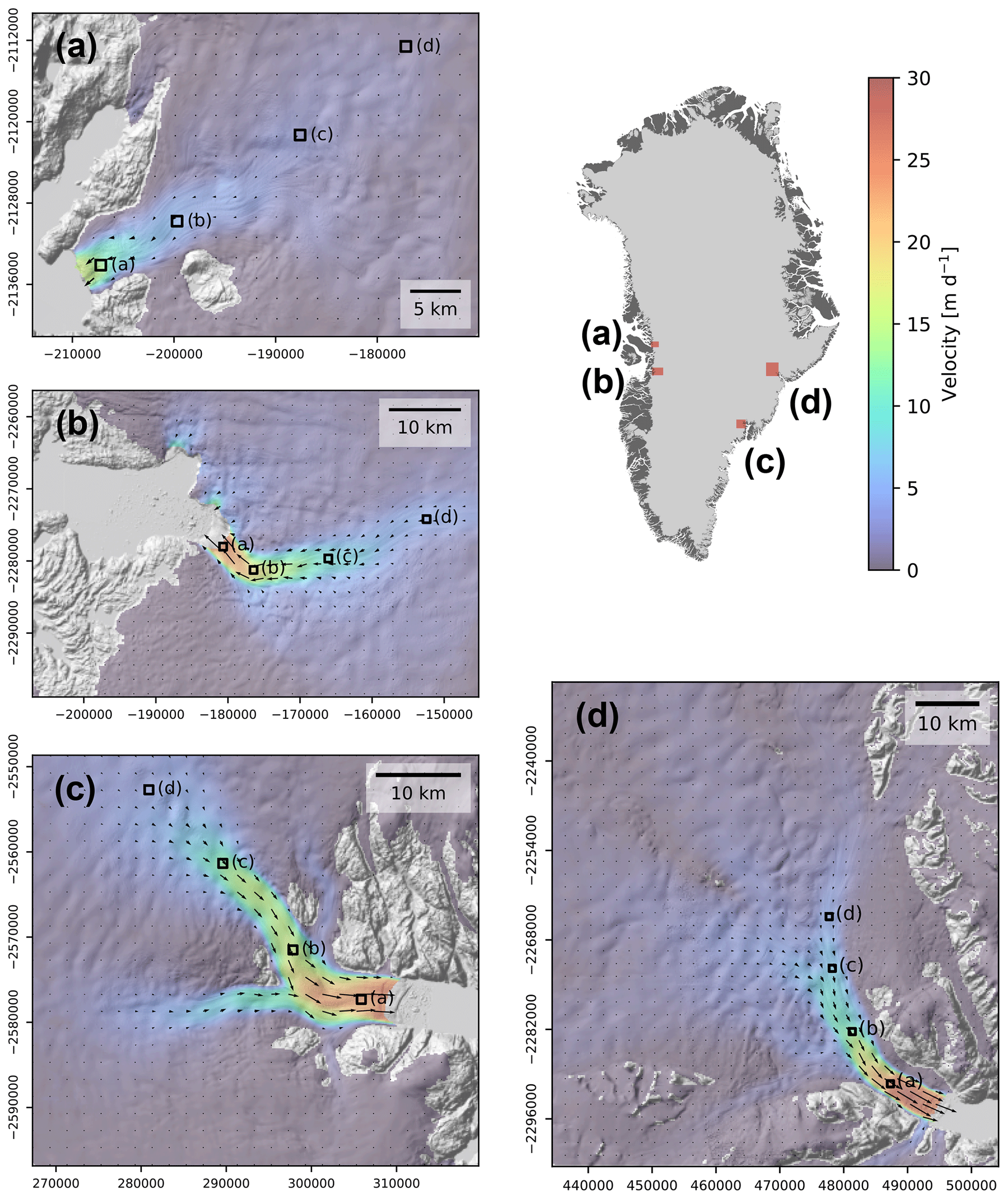
Figure 1 Reference velocity fields (median velocity of repeat-orbit pairs; see Sect. 2.1.2) for the four marine-terminating glaciers presented in this paper, ordered anti-clockwise from north: (a) Store Glacier, (b) Jakobshavn Isbræ, (c) Helheim Glacier, and (d) Kangerlussuaq Glacier. The 1 km ×1 km sample sites a–d are marked for each glacier – see Table S2 for precise coordinates. Backgrounds are GrIMP DEM hillshades (Howat et al., 2017); coordinates in NSIDC Sea Ice Polar Stereographic North (EPSG:3413). Inset: location in Greenland of all outlet glacier AOIs (red).

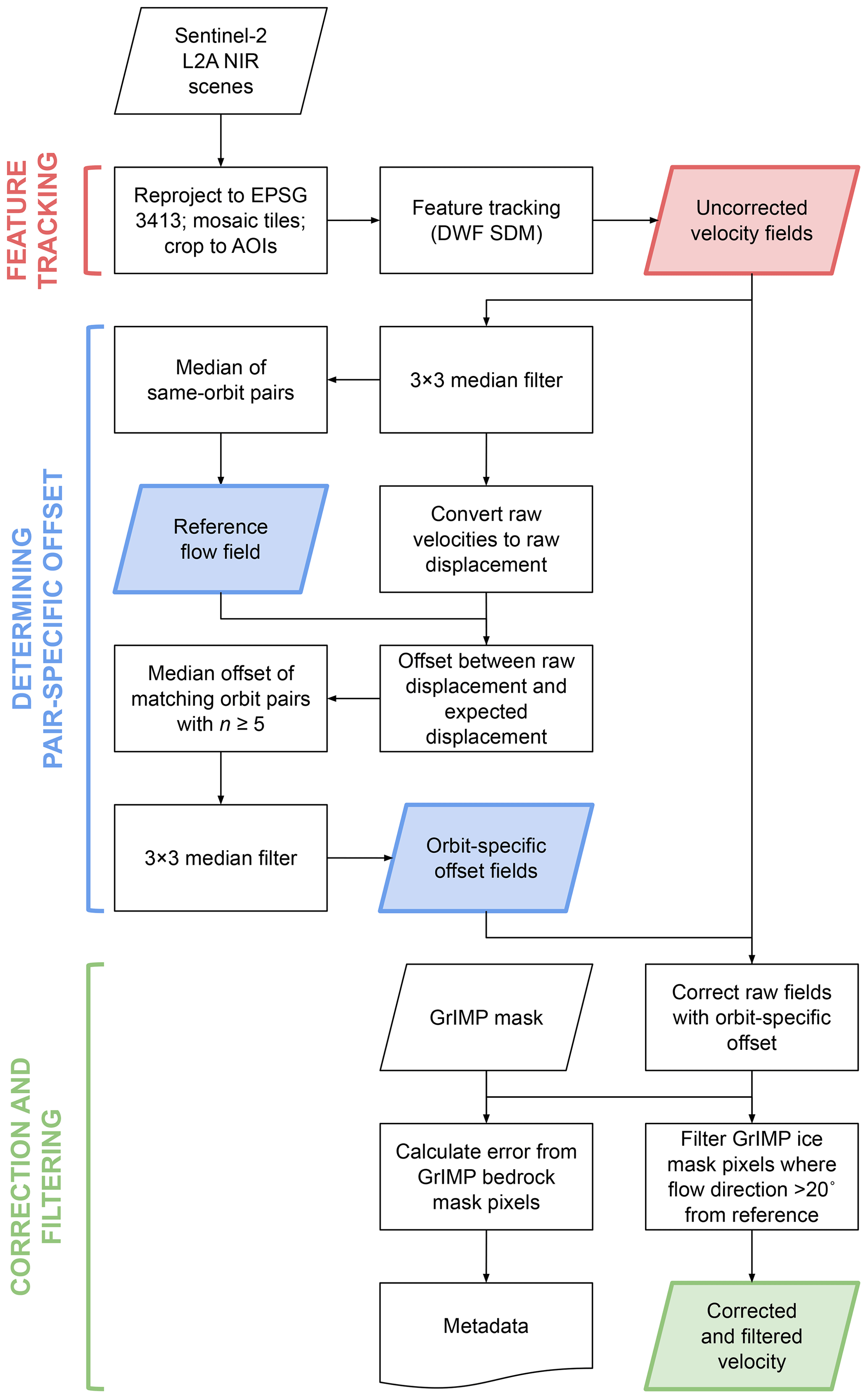
Figure 2 Workflow for deriving corrected and filtered glacier velocity fields from Sentinel-2 Level-2A data.

As orthorectification error is a function of satellite geometry, it should result in a consistent offset (in units of absolute displacement rather than velocity) across all velocity fields generated from the same relative orbit pairs. We assume that other errors in the velocity field (e.g. image matching error, coregistration error) are (a) random and (b) do not correlate with specific relative orbit pairings. Hence, by drawing from a large base dataset, we can infer the average orthorectification error over the study period for specific relative orbit pairs by measuring the average offset between (i) the ice displacement measured from Sentinel-2 scenes and (ii) the expected displacement from a reference velocity field. We refer to this difference as the orbit-pair offset field and subtract it from measured fields to generate final corrected fields (Fig. 2).

2.1 Data production

2.1.1 Velocity field production

Data are produced at four marine-terminating glaciers, matching the spatial extent of the areas of interest (AOIs) in the MEaSUREs Selected Glacier Site Velocity Maps from Optical Images collection (Howat, 2020). We downloaded all bottom-of-atmosphere corrected Level-2A (L2A) Sentinel-2 data with a cloud cover <50 % from the Amazon Web Services (AWS) Registry of Open Data using the sat-search STAC API (https://github.com/sat-utils/sat-search, last access: 29 February 2022). Sentinel-2 data are staged using a pre-defined tiling scheme based on the Military Grid Reference System (MGRS). The pre-processing pipeline includes subsetting Sentinel-2 tiles for each glacier AOI, reprojecting the raster to a common WGS 84/National Snow and Ice Data Centre (NSIDC) Sea Ice Polar Stereographic North (EPSG:3413) projected coordinate system, mosaicking the adjacent overlapping tiles, and finally clipping the mosaicked raster to the glacier AOI. We only considered scenes until 23 August 2021, when the L1C orthorectification process switched to a new geolocation procedure and underlying DEM (Sect. 4.3).

Velocity fields at 100 m resolution were produced using feature tracking methods, performed using a directional weighted filtering (DWF) algorithm based on the Surface Extraction from TIN-based Search-space Minimization (SETSM) approach (Noh and Howat, 2019). The method was originally developed for precisely estimating the surface displacement map (SDM) by compensating for relative sensor model biases (minimising co-registration errors) and removing orthorectification errors caused by height changes through true DEMs. For the purpose of this research, we modified the algorithm to use orthorectified images directly, and we applied the relative sensor model bias compensation module as co-registrations. For co-registration, we define the off-ice region using the GrIMP ice mask (Howat et al., 2014). The SDM processing is fully automated except in using an a priori, or seed, velocity field to specify maximum displacements for determining the initial resolution in the coarse-to-fine processing scheme (Noh and Howat, 2019). Here, we used InSAR-derived velocity fields between 2016 and 2017 (Joughin, 2021b) as the seed.

2.1.2 Estimating orbit-pair offsets

Velocity fields are grouped by the relative orbits of their respective source image pairs. Pairs of images acquired from the same relative orbit are hereafter referred to as repeat-track pairs, and those from different relative orbits as cross-track pairs. For any given outlet glacier, certain combinations of orbit pairs may have anywhere from a few to >100 velocity fields.

A reference flow field is constructed using the median U and V velocity values (in x and y EPSG:3413 Polar Stereographic North grid directions) from all (2017–2021) repeat-track velocity fields. Before processing, uncorrected velocity fields are filtered using a 3×3 median filter to reduce noise. For individual velocity fields, the expected displacement is calculated from these reference flow fields and the temporal baseline of the scene pair. The offset between the uncorrected displacement and the expected displacement is then calculated. Empirical orbit-pair offset fields are generated as the median offset for each orbit pair. Where these offset fields are constructed from fewer than five velocity fields, their quality is notably degraded. Hence, where a particular orbital pair has fewer the five observations, an empirical offset field is not constructed, and the velocity fields are not processed further.

We note that over the course of the study period ongoing glacier surface elevation change will continue to change Δh, and hence the orthorectification error will not be constant. However, our method of estimating orthorectification error across the entire 2017–2021 study period implicitly assumes a constant Δh. We could improve this assumption by assessing offsets on shorter timescales – such as annually – but shorter timescales (smaller sample sizes) result in a notable reduction in the number of cross-track pairs available for correction (i.e. satisfying our threshold of five available velocity fields) and a lower quality of offset fields even for cross-track pairs where sufficient data are available. However, given the large initial Δh values, surface elevation change over the study period likely has a negligible impact on the orthorectification error. Using annual surface elevation change rates between 2003–2019 from Smith et al. (2020) as approximations, maximum surface elevation change rates at our study sites range between −0.3 (Store Glacier) and −3.6 m a⁻¹ (Kangerlussuaq Glacier). Maximum estimated $\left|\mathrm{\Delta }h\right|$ values (Sect. 3.1), which roughly correlate with these values, range between ∼160 and ∼400 m. Over the 4-year study period, this results in a potential time-dependent error in Δh of between 0.3 % and 2.2 % at our study glaciers. Applying these uncertainties to typical maximum offsets (directly correlated with Δh) of between 40 and 60 m shows that, even using worst-case assumptions, offset vector errors range between ±0.2 and ±1.3 m, values which are subsumed by other error terms (e.g. miscorrelation and coregistration).

Figure 3 Median offset between measured displacement and expected displacement (from reference velocity field) for different orbital pairs at Helheim Glacier. Magnitude is shown in colour; vectors are shown as white arrows. The orbital geometry of the constituent relative orbits is visualised in Fig. S2.

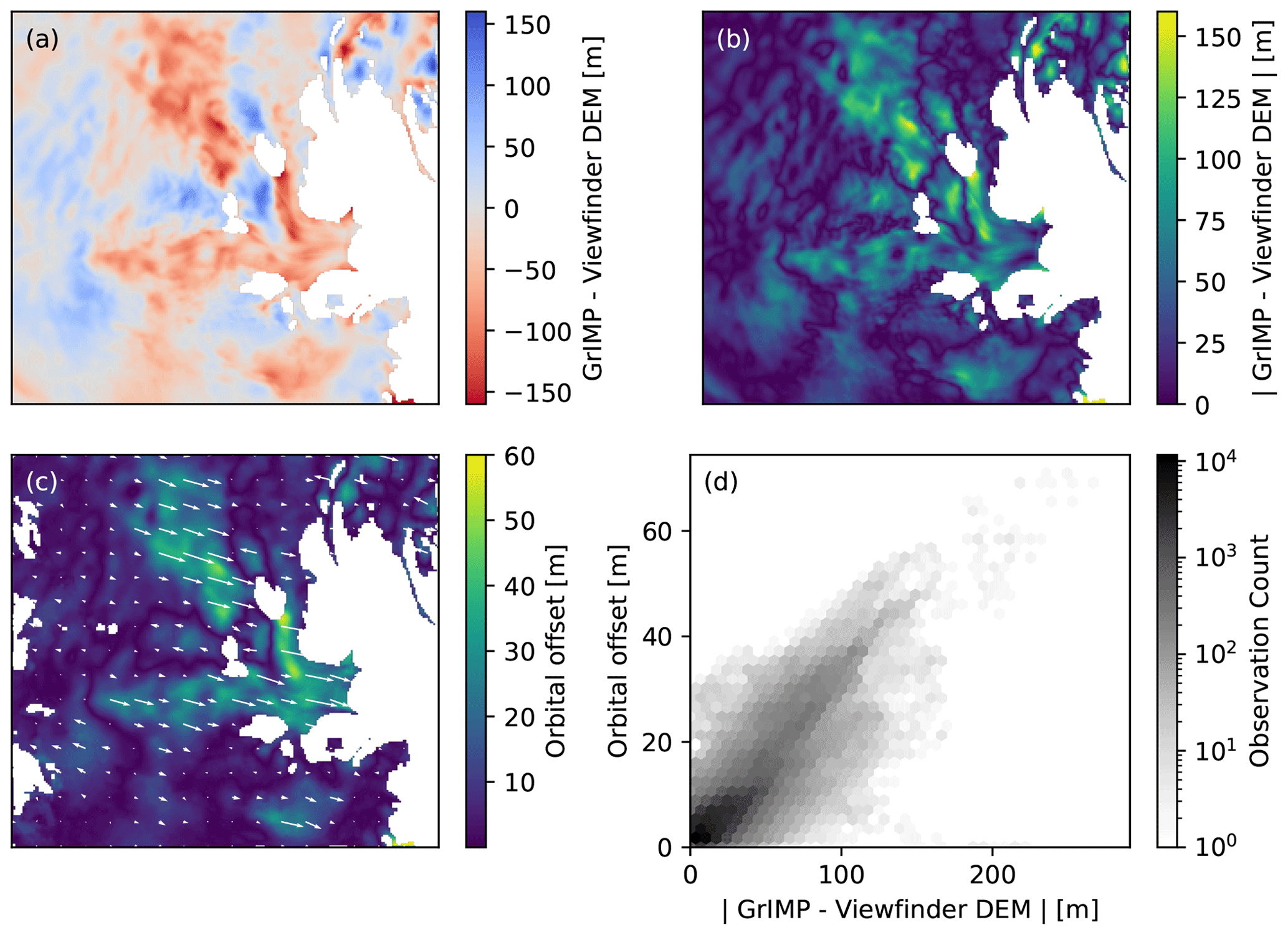
Figure 4 Comparison between DEM vertical differences and velocity offset for Helheim Glacier. (a) DEM difference between the GrIMP DEM and the Viewfinder DEM. (b) Absolute vertical difference between the Viewfinder DEM and GrIMP DEM. (c) Median offset between the measured displacement and expected displacement for velocity fields taken from relative orbits 053 and 139 (identical to Fig. 3c). (d) Hexbin density plot comparing the absolute vertical differences between the Viewfind DEM and GrIMP DEM with the empirically determined orbital displacement.

2.1.3 Velocity correction and filtering

Once orbit-pair offsets have been constructed, uncorrected velocity fields are converted to absolute displacement, corrected using the appropriate orbit-pair displacement offset field, and converted back to velocity. Displacements are corrected only over ice as defined in the GrIMP mask, as our correction scheme is designed to correct for surface elevation change, which we assume is largely negligible outside of the ice sheet boundaries. Due to changing ice boundaries at marine-terminating locations, areas within the GrIMP ocean mask are not filtered or removed, but ice velocities beyond the extent of the GrIMP ice mask should not be considered reliable.

To remove erroneous velocity measurements, areas within the GrIMP ice mask are filtered where flow directions are $>\mathrm{20}{}^{\circ }$ offset from the reference flow field. If, after filtering, no data remain (<1 % of the ice area has valid velocity measurements), the field is discarded and no output data are generated.

2.1.4 Error assessment

A first-order estimate of error is taken as the root mean square error (RMSE) of the absolute velocity of the bedrock area (as defined by the GrIMP bedrock mask). RMSEs tended to be low, with the median RMSE consistently beneath <0.5 m d⁻¹ for the study glaciers discussed in this paper (Fig. S1 in the Supplement). Additionally, the mean and standard deviation of the U and V velocity fields of the bedrock area are also recorded, in order to assess systematic error within individual flow fields due to poor co-registration for example. Where the mean of the U or V velocity is greater than 1 standard deviation away from zero, the field is considered to have a systematic error and is not included for presentation in this study (Sect. 2.2).

2.2 Data presentation

2.2.1 Sampling

To present time series of glacier surface velocity, we sample four sites of increasing distance from the calving front at each of our sample glaciers (Fig. 1; Table S1 in the Supplement). We sample across a 1 km ×1 km area, calculating the median velocity across this sample region. We filter out data points where <70 % of the sample region contains data, or where the RMSE error estimate is >5 m d⁻¹. We further filter fields where the temporal baseline is only 2 d, where errors were significantly greater than any other baselines (Fig. S3).

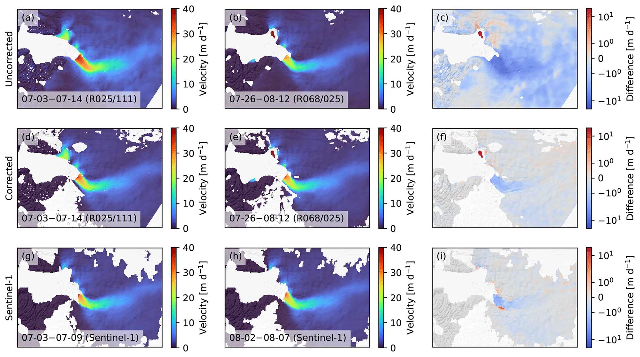
Figure 5 Velocity difference maps at Jakobshavn over a period of summer slowdown in 2019 (see Figs. 6 and 7). (a) Velocity field pre-slowdown, from uncorrected Sentinel-2 feature tracking. (b) Velocity field post-slowdown, from uncorrected Sentinel-2 feature tracking. (c) Difference between pre- and post-slowdown from uncorrected Sentinel-2 feature tracking. (d–f) Same as (a–c), but for corrected Sentinel-2 feature tracking. (g–i) Same as (a–c), but for contemporaneous Sentinel-1 speckle tracking. Note log scale used on difference maps. Backgrounds are GrIMP DEM hillshades (Howat et al., 2017).

2.2.2 Gaussian process regression

The output from our velocity correction process produces a dense time series of varying error estimates. Hence, we use Gaussian process (GP) regression (Rasmussen and Williams, 2006; Hugonnet et al., 2021) to estimate a continuous uncertainty-bounded time-series velocity from our sampled time-series observations. Two particular properties of GP regression make it useful for the current application: (i) the Bayesian nature of the method accommodates the incomplete velocity record, producing a smooth, nonlinear, interpolated output, and (ii) the probabilistic model can incorporate uncertainty estimates and provides an empirical confidence interval to predictions.

We performed GP regression using the GaussianProcessRegressor() implementation in the Python scikit-learn library. We model ice velocity as the sum of two kernels (covariance functions) representing seasonal and short-term variability. Our implementation follows Rasmussen and Williams (2006), ignoring long-term variability over the 5-year period we assess. Seasonal variability is incorporated as the product of an exponential sine squared kernel (ExpSineSquared()) and a radial basis function kernel (RBF()). The exponential sine squared kernel has a fixed periodicity of 1 year and the length scale as a free parameter. The radial basis function kernel has a free length scale. We implement short-medium term variability as a rational quadratic kernel (RationalQuadratic()), with free length scale and alpha (controlling the diffusivity of the length scale) parameters. Finally, we incorporate velocity error estimates (Sect. 2.1.3) into modelling directly via the alpha parameter of the GaussianProcessRegressor().

2.3 Supplementary data

As orthorectification errors scale with Δh, we compare generated offset maps to DEM difference as a proxy for Δh. The first DEM is the Viewfinder Panoramas 3^′′ DEM for Greenland (Version 1) (de Ferranti, 2014; hereafter the “Viewfinder DEM”). Kääb et al. (2016) inferred that the Viewfinder DEMs likely shared source data with the PlanetDEM for a test site in northern Norway. The second DEM is the GrIMP DEM from GeoEye and WorldView Imagery (Version 1) (Howat et al., 2014, 2017; hereafter the “GrIMP DEM”), which was produced from imagery between 2009–2015.

We compare our generated velocity fields to two other public datasets. To compare with medium-resolution SAR velocity fields, we make use of MEaSUREs Greenland 6 and 12 d Ice Sheet Velocity Mosaics from SAR (Version 1) velocity fields from speckle-tracked Sentinel-1 data (Joughin et al., 2018; Joughin, 2021a). These were downloaded from the NSIDC data portal. To compare with optical velocity fields derived from Landsat 8 imagery, we make use of the ITS_LIVE dataset (Gardner et al., 2018, 2021). These were downloaded using the ITS_LIVE API, and, to match our Sentinel-2 data thresholds, filtered to velocity fields where (i) the maximum interval between data pairs was 30 d and (ii) at least 1 % of the data contained valid pixels. For both Sentinel-1 and Landsat 8 fields, we extracted time-series data in the same way as for Sentinel-2 data: i.e. filtering to data that cover at least 70 % of the 1 km ×1 km sample region and <5 m d⁻¹ error.

3 Results

3.1 Orbital offset generation

Empirically determined systematic offsets can reach values on the order of tens of metres at outlet glaciers around Greenland. Comparing offset fields constructed for various orbit pairs at Helheim Glacier (Fig. 3) shows that the behaviour of empirical offset fields are consistent with theory. Offset fields for repeat orbit pairs (Fig. 3a, e, i) have negligible offset, whilst the offset is largest for the cross-track pairs from relative orbits 053 and 139 (Fig. 3c, g), which have the greatest distance between their respective orbital paths (Fig. S2). Empirical offset vectors are, to within reasonable error, uniformly parallel and occur along the epipolar line of the satellite pair viewing geometry (Figs. 3, cf. S2), consistent with the hypothesis that these systematic errors occur due to orthorectification error in the off-nadir direction.

If the measured offsets are due to orthorectification error, they should directly correlate to the Δh between the times of DEM and image acquisition. We can thus validate that our offsets are meaningful by comparing them to the DEM difference between the Viewfinder DEM, which we use as a proxy for the PlanetDEM (Sect. 2.3), and version 2 of the GrIMP DEM, which acts as our reference elevation, or at least a closer approximation to the surface elevation at the time of image acquisition (Fig. 4). The spatial pattern of $\left|\mathrm{\Delta }h\right|$ (Fig. 4b) matches the magnitude of the orbital offset (Fig. 4c), with a strong, positive correlation (R²=0.67, p<0.01) between the two variables (Fig. 4d). The direction of the offset (white vectors in Fig. 4c) is also predicted by the direction of Δh (Fig. 4a): where Δh values are negative, offset error occurs in the ESE direction (towards relative orbit 053), whereas positive Δh values occur where offset errors are in the WNW direction (towards relative orbit 139).

The efficacy of the orbital correction fields is visualised for an example case at Jakobshavn Isbræ (Fig. 5), which shows the relative ability of corrected and uncorrected glacier velocity fields to properly capture the magnitude and extent of a summer slowdown occurring in late July 2019 (see also Figs. 6 and 7 for time series of this event). In the uncorrected velocity fields (Fig. 5a and b), orthorectification error in the cross-track velocity fields (relative orbits 025/111 and 068/025 respectively) introduces an apparent difference in the final velocity field in excess of 10 m d⁻¹ at the calving front and 2 m d⁻¹ even tens of kilometres inland, a rate of change that is unphysical. After correction (Fig. 5d and e), this change is reduced to ∼2–3 m d⁻¹ at the front and negligible amounts inland (Fig. 5f), an observation that is in line with contemporaneous Sentinel-1 observations (Fig. 5g–i).

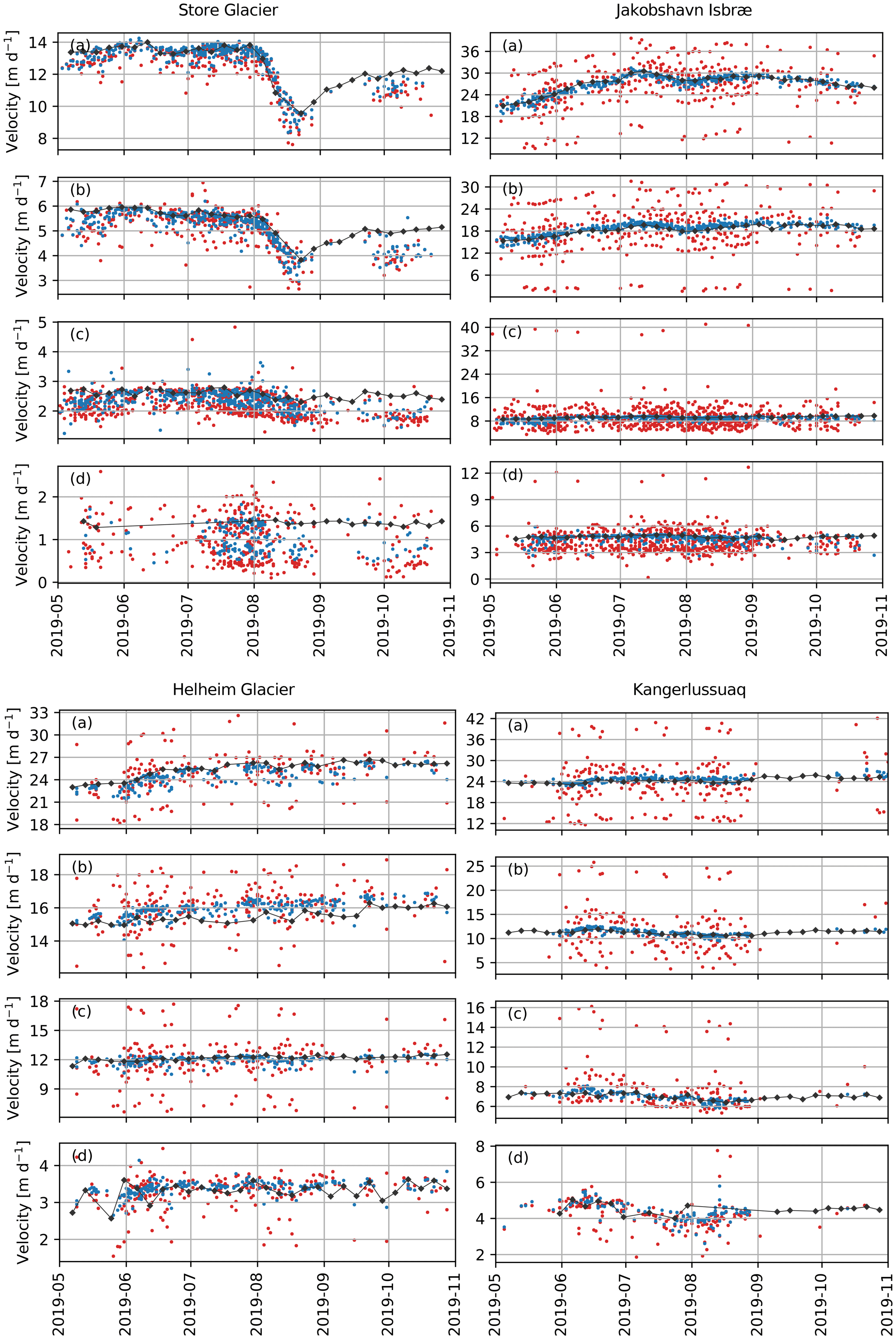
Figure 6 Corrected (blue) and uncorrected (red) velocity time series for four sample glaciers in 2019. Top to bottom are points (a–d) in Fig. 1. The black line and diamonds mark the MEaSUREs Sentinel-1 velocity dataset for comparison.

3.2 Ice velocity time series

For the sampled 1 km ×1 km sectors of our four study glaciers, we compare our corrected Sentinel-2 data against other data sources. Comparing our corrected velocity data to the uncorrected dataset shows the improvement that our empirical correction has (Fig. 6). Uncorrected data show a characteristic error distribution, with points offset from the Sentinel-1 -derived velocities based on their constituent orbit pairs and their temporal baseline. Prior to correction, short-baseline pairs are increasingly offset from the reference dataset value, even where orbit pairs are identical (Fig. S4). This is because orthorectification error is an absolute displacement offset and as such becomes a higher relative error component of short-baseline velocities. In all cases, the corrected velocity data converge near the reference Sentinel-1 time series. The correction is greatest for observations at Jakobshavn Isbræ and Kangerlussuaq Glacier, where Δh values are the largest.

The high density of data points reveals a noisy dataset compared to the SAR-derived data. The use of GP regression highlights an effective way of interpolating a continuous time series from this dataset (blue line in Fig. 7), whilst accounting for sample-specific error values and time-variable data densities. Across all sites, the median difference between the Sentinel-1 record and the GP fit is 0.08 m d⁻¹, 68 % (95 %) of values lie within 0.41 (0.73) m d⁻¹ of one another, and 90.5 % of Sentinel-1 values lie within the error of the Sentinel-2 GP fit (Table S2). These differences, on the order of decimetres, align with our error estimates from off-ice displacement of between 0.3 and 0.5 m d⁻¹ on average (Fig. S1). The lowest level of agreement between the two datasets occurs at Helheim Glacier point b, where only 52.3 % of Sentinel-1 velocity values lie within error of the Sentinel-2 GP fit, and the Sentinel-1 record is, on average, 0.47 m d⁻¹ slower than that of the GP fit.

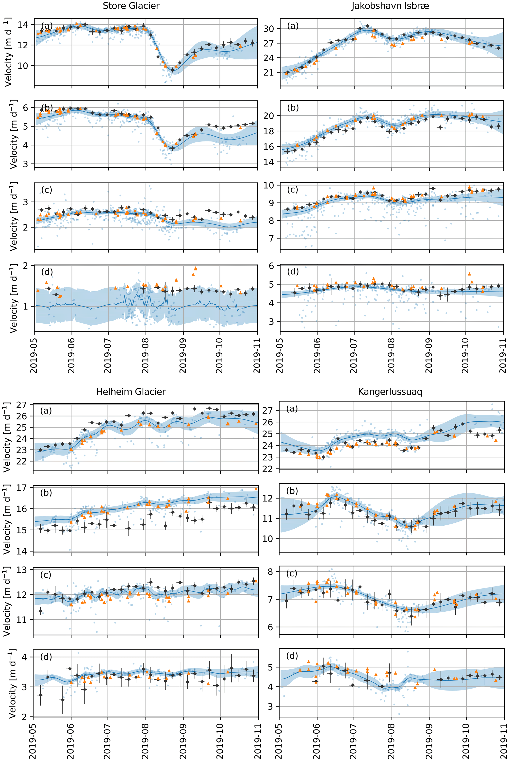
Figure 7 Corrected Sentinel-2 (blue dots), ITS_LIVE Landsat-8 (orange triangles), and MEaSUREs Sentinel-1 (black diamonds) velocity time series for four sample glaciers in 2019. Top to bottom are points (a–d) in Fig. 1. The blue line marks the output of the Gaussian process regression, with the blue shading marking the 2σ uncertainty bound.

This high level of agreement also occurs in comparison with the ITS_LIVE dataset derived from optical Landsat 8 imagery (orange triangles in Fig. 7). Across all sites, the median difference between the ITS_LIVE record and the GP fit is 0.12 m d⁻¹, 68 % (95 %) of values lie within 0.29 (0.63) m d⁻¹ of one another, and 87.0 % of values lie within error of each other (Table S3). The increased density of the Sentinel-2 record relative to the Landsat 8 record allows for a higher temporal precision in identifying rapid drainage events. For instance, the summer slowdown at sites a and b at Store Glacier are not as not well captured in the Landsat 8 or Sentinel-1 records, where a sparse record means that the timing of the slowdown often appears to take more than a month, whilst the dense Sentinel-2 dataset and the GP fit show the slowdown to occur on a timescale of ∼2 weeks (Fig. S5). However, the Landsat 8 record displays a higher precision at lower velocity values (sub-4 m d⁻¹, e.g. site d at Store Glacier), likely because any errors in the empirically derived displacement field have greater relative influence at low flow velocities.

4 Discussion

4.1 Data quality

In the absence of empirical correction, orthorectification errors can result in errors in excess of 10 m d⁻¹ in short-baseline velocity fields at Greenlandic outlet glaciers (Figs. 5, 6). As orthorectification error is linearly proportional to Δh between the orthorectification DEM and the true glacier surface (Fig. 4), errors are greatest at glaciers where ice surface elevation has changed the most. This is exemplified by Store Glacier, which is notable for its long-term stability induced by a sill at the glacier terminus (e.g. Morlighem et al., 2016) and has relatively low orthorectification errors prior to correction (Fig. 6).

The empirical corrections described in this paper demonstrably reduce the influence of systematic orthorectification error on Sentinel-2-derived glacier velocity fields, reducing the variance from the order of metres to decimetres (Figs. 6, 7). This allows for the incorporation of cross-track pairs into the glacier velocity time series, increasing the temporal density of observations, in particular for pairs with short (<10 d) baselines, by as much as a factor of 7 (Fig. S4b). The temporal density of observations means that short-term variations in speed, such as the slowdown at the terminus of Store Glacier, can be well resolved (Fig. S5). The noise of the dataset highlights the utility of effective filtering and time series modelling, such as GP regression (Fig. 7), in extracting a continuous velocity estimate – following other studies that have made use of, for example, Kalman filtering (King et al., 2018) to similar effect – and it provides the advantage of a greater accuracy through the synthesis of multiple estimates. GP fits over the four glaciers assessed here differ from Sentinel-1 observations by, on average, only 0.08 m d⁻¹, and 90.5 % of Sentinel-1 values lie within the GP fit error (Rable S2). Unlike monthly averaging, the use of GP regression retains the ability to capture short-term variation at approximately weekly timescales and provides a time-varying confidence interval based on training data uncertainty and coverage.

The data display high agreement with comparative datasets sourced from Sentinel-1 and Landsat 8 (Fig. 7). Although Sentinel-1 has been presented as a “true” reference velocity in this study, it is of note which two will vary when only two of the three records presented agree with each other: contrast, for instance, Helheim site b (Sentinel-2 and Landsat 8 agree), Jakobshavn site a (Sentinel-2 and Sentinel-1 agree), and Kangerlussuaq site a (Sentinel-1 and Landsat 8 agree). All three methods are orthorectified using different DEMs whose ages, accuracies, and resultant Δh values are variable. As such, it is likely that systematic biases are present in all three datasets and are spatially variable on a kilometre scale. However, the characteristics of the cross-track Sentinel-2 dataset will make it advantageous over Landsat 8-derived datasets in scenarios where a high density of observations is required, as the increased observation frequency will allow for a greater chance of successful image pairs over critical dynamic periods, such as the early melt season acceleration and late summer slowdown. In contrast, individual Landsat 8 velocity fields appear to be more precise and may be preferable when the accuracy of individual velocity fields are necessary (e.g. comparing early and late season velocities). Sentinel-2 also provides a temporal advantage over Sentinel-1 datasets, which are limited to a fixed 6 d repeat cycle, and may also provide a valuable alternative for applying to small and steep glaciers, such as in high mountain regions, where the use of synthetic aperture radar for velocity extraction can be challenging (e.g. Paul et al., 2022).

4.2 DEM origin

The differencing of orbital pair offsets from a reference flow field has been shown to be an effective method of reconstructing systematic orthorectification errors when the underlying DEM is not available. Furthermore, we show that orthorectification errors over Helheim Glacier are consistent with Sentinel-2 data being orthorectified using data sources present in the Viewfinder Panoramas 3^′′ DEM (de Ferranti, 2014). This finding agrees with that of Kääb et al. (2016), who found similar agreement between a Δh estimated from the Viewfinder DEM and Sentinel-2 offsets for a test site in northern Norway. Further testing is required to establish if the Viewfinder DEM and PlanetDEM data sources are consistent across broader regions of Greenland and the high latitudes, but if they are then the freely available Viewfinder DEM opens new avenues for deriving high-latitude Sentinel-2 orthorectification error from analytical methods (Ressl and Pfeifer, 2018). To do so would require not only the Viewfinder DEM but also a “true” glacier surface elevation DEM contemporaneous to image acquisition, which is difficult to acquire in rapidly changing sectors of the cryosphere. Here, we highlight the utility of time-evolving DEMs and the potential of ArcticDEM strips (Porter et al., 2018) and monthly/annual composites thereof to address this challenge in the future.

4.3 Future datasets

The empirical offsets derived in this study are only applicable up to 23 August 2021. On this date (or 30 March 2021 for coverage of Europe and Africa), L1C/L2A Sentinel-2 products switched to an improved geometric refinement with two major changes: (i) co-registration of scenes to a Global Reference Image (GRI) and (ii) the use of a new DEM, the Copernicus DEM at 90 m resolution (“GLO-90”), for topographic correction. This new DEM is based on 2011–2015 radar satellite data acquired during the TanDEM-X mission, meaning there will be a discontinuity in Δh between the pre- and post-August 2021 data.

There is no currently announced reprocessing of the Sentinel-2 archive with the new geometric refinements (see, for example, Landsat Collection 2), so this discontinuity between pre- and post-2021 data will remain into the future. As such, the method outlined here remains applicable for the correction of Sentinel-2-derived glacier velocity across the wider cryosphere for Sentinel-2 L1C and L2A data between 2015–2021. The more recent dataset will reduce the value of Δh and as such the orthorectification error in the new datasets – although as the DEM used for orthorectification consists of pre-2015 data, some orthorectification error will remain. As such, offset fields such as those calculated in this study will need to be calculated separately for the pre- and post-2021 data. Additionally, the lower Δh value will likely invalidate the assumption we make in this study that further elevation change will have a negligible impact on our assumption of stable geometry. However, GLO-90 is available for public download (European Space Agency, 2021), allowing for correction via analytical methods. In combination with the opportunities we highlight in Sect. 4.2, this provides a framework for the production of a continuous Sentinel-2 velocity dataset from 2016–present with cross-track velocities corrected analytically according to their underlying DEM.

5 Conclusions

By taking advantage of the complete Sentinel-2 record between 2017–2021, we demonstrate an empirical method of correcting for systematic orthorectification error in glacier velocity fields derived from cross-track image pairs in large-scale datasets. The method is simple and computationally undemanding, whilst allowing for spatially continuous glacier velocity fields to be constructed without limitations introduced by satellite and flow geometry. This method is used to produce a complete dataset of glacier velocity for four key marine-terminating glaciers across the Greenland Ice Sheet. Comparison with alternative datasets highlights the key advantages of the high temporal frequency of Sentinel-2 imagery, but this density of data also necessitates the use of statistical techniques to account for noise and uncertainty in the dataset. Furthermore, we use this method to identify a likely publicly available data source for the DEM data used to orthorectify Sentinel-2 scenes over Greenland between 2015–2021, which will be useful for future studies concerned with orthorectification error in the region. The transition to a new geometric refinement method for Sentinel-2 scenes beyond August 2021 will require new correction offsets to be generated, but the transition to a publicly available DEM (and the identification of 2015–2021 data sources in this study) provides the opportunity for this to occur through analytical rather than empirical methods.