the Creative Commons Attribution 4.0 License.
the Creative Commons Attribution 4.0 License.
 | 24 Jan 2022
Cross-platform classification of level and deformed sea ice considering per-class incident angle dependency of backscatter intensity
Wenkai Guo
Polona Itkin
Johannes Lohse
Malin Johansson
Anthony Paul Doulgeris
Wide-swath C-band synthetic aperture radar (SAR) has been used for sea ice classification and estimates of sea ice drift and deformation since it first became widely available in the 1990s. Here, we examine the potential to distinguish surface features created by sea ice deformation using ice type classification of SAR data. Also, we investigate the cross-platform transferability between training sets derived from Sentinel-1 Extra Wide (S1 EW) and RADARSAT-2 (RS2) ScanSAR Wide A (SCWA) and fine quad-polarimetric (FQ) data, as the same radiometrically calibrated backscatter coefficients are expected from the two C-band sensors. We use a novel sea ice classification method developed based on Arctic-wide S1 EW training, which considers per-ice-type incident angle (IA) dependency of backscatter intensity. This study focuses on the region near Fram Strait north of Svalbard to utilize expert knowledge of ice conditions during the Norwegian young sea ICE (N-ICE2015) expedition. Manually drawn polygons of different ice types for S1 EW, RS2 SCWA and RS2 FQ data are used to retrain the classifier. Different training sets yield similar classification results and IA slopes, with the exception of leads with calm open water, nilas or newly formed ice (the “leads” class). This is caused by different noise floor configurations of S1 and RS2 data, which interact differently with leads, necessitating dataset-specific retraining for this class. SAR scenes are then classified based on the classifier retrained for each dataset, with the classification scheme altered to separate level from deformed ice to enable direct comparison with independently derived sea ice deformation maps. The comparisons show that the classification of C-band SAR can be used to distinguish areas of ice divergence occupied by leads, young ice and level first-year ice (LFYI). However, it has limited capacity in delineating areas of ice deformation due to ambiguities between ice types with higher backscatter intensities. This study provides reference to future studies seeking cross-platform application of training sets so they are fully utilized, and we expect further development of the classifier and the inclusion of other SAR datasets to enable image-classification-based ice deformation detection using only satellite SAR.
- Article
(22034 KB) - Full-text XML
- BibTeX
- EndNote


The general thinning of Arctic sea ice in recent decades has led to reduced internal strength (Landrum and Holland, 2020), which together with increased wind forcing (as indicated by atmospheric reanalyses) has caused accelerated ice drift speed (Spreen et al., 2011) and hence increased ice deformation (Rampal et al., 2009, 2011; Itkin et al., 2017). As surface features created by ice deformation, e.g., lead edges, rafted ice and pressure ridges, are the primary snow-trapping sea ice surface types (Liston et al., 2018), the shifting regime of Arctic sea ice deformation will directly impact snow accumulation and thus affect heat fluxes through ice, thereby influencing winter sea ice growth (Sturm et al., 2002). Also, ice deformation influences ice surface and bottom roughness and thus affects the transfer of momentum between the atmosphere and the ocean (Cole et al., 2017; Martin et al., 2016), preconditions the ice layer for more lateral melt (Arntsen et al., 2015; Hwang et al., 2017; Graham et al., 2019), and increases ice drift speed due to reduced floe sizes following ice breakups (Toyota et al., 2006; Steer et al., 2008; Asplin et al., 2012). Additionally, ice deformation has a significant impact on ice primary productivity, as it provides a sheltered growth environment for ice flora and fauna in deformed ice (Gradinger et al., 2010; Fernández-Méndez et al., 2018; Graham et al., 2019) and favorable light conditions under lead ice (Assmy et al., 2017), creating biological hotspots. Reliable examination of sea ice deformation is therefore crucial for the evaluation and modeling of Arctic sea ice changes.
Sea ice deformation is traditionally estimated from spatial derivatives of ice motion using in situ, airborne and spaceborne data (e.g., Hutchings et al., 2011; Itkin et al., 2017, 2018; Bouillon and Rampal, 2015). However, consistent Arctic-wide monitoring of sea ice deformation can only be achieved through satellite remote sensing. Wide-swath synthetic aperture radar (SAR) data, e.g., RADARSAT-1 (RS1, 1995 to 2013), RADARSAT-2 (RS2, 2008 to present), the recently launched RADARSAT Constellation Mission (RCM, 2019 to present) and Sentinel-1A/B (S1, 2014 to present) data, have been used to generate large-scale ice drift and deformation fields (e.g., Marsan et al., 2004; Komarov and Barber, 2014; Korosov and Rampal, 2017; Howell et al., 2018), benefiting from large spatial coverage and good temporal resolution. For example, the RADARSAT Geophysical Processor System (RGPS; Kwok, 1998) generates the most widely used sea ice motion and deformation dataset using cross-correlation-based ice tracking on RS1 data for the western Arctic from 1997 to 2008 (Raney et al., 1991). Data from other types of satellite sensors, e.g., visible, infrared, and microwave radiometers and radar scatterometers, can also be used to generate ice drift fields with coarser resolution through feature tracking algorithms, for example those used by the National Snow and Ice Data Center (NSIDC; Tschudi et al., 2020) and the Ocean and Sea Ice Satellite Application Facility (OSI SAF; Cavalieri et al., 2011; Lavergne, 2016; Dybkjaer, 2018).
In addition to sea ice deformation retrieval from ice motion, the potential of separating areas of deformed and level ice as classes in wide-swath SAR image classification is valuable, as the automated or semi-automated nature of such methods permits fast processing of data with large spatial and temporal coverage. Various supervised and unsupervised SAR sea ice classification methods have been developed, as reviewed by, for example, Zakhvatkina et al. (2019). Under the same radar parameters, the intensity of SAR backscatter on sea ice is the combined signal from several scattering mechanisms, of which surface scattering is the dominant factor (Onstott, 1992; Moen et al., 2013). Surface scattering is controlled by surface parameters including roughness and dielectric properties. Therefore, the separation of level and deformed ice, which have distinctly different surface roughness levels, is theoretically achievable through the classification of SAR backscatter intensities. Studies have isolated deformed ice using the classification of airborne and fully polarimetric high-resolution satellite SAR data (e.g., Casey et al., 2014; Herzfeld et al., 2015) and linked sea ice roughness to wide-swath SAR backscatter intensities through correlation analyses, thus mapping sea ice deformation (Cafarella et al., 2019; Segal et al., 2020; Toyota et al., 2020). Gegiuc et al. (2018) estimated the degree of ice ridging from the classification of texture features from segmented RS2 ScanSAR Wide A (SCWA) data. However, no study has specifically targeted separating level from deformed ice from the classification of wide-swath SAR backscatter intensities.
This study investigates the feasibility of such a task with an ultimate goal of Arctic-wide monitoring of sea ice deformation. In this context, a classification method consistently applicable to multiple satellite platforms is desirable to utilize their respective advantages. This study is a first step towards this goal, which explores how the cross-platform application of a SAR classifier between S1 and RS2 data is influenced by their comparative SAR characteristics. This is achieved by examining the transferability of classification training sets between these two sensors. S1 and RS2 are widely used for sea ice monitoring, and their wide-swath acquisition modes provide extensive spatial and temporal coverage for Arctic-wide sea ice analyses (Zakhvatkina et al., 2019). This transfer learning process is theoretically feasible as the two sensors are expected to yield the same radiometrically calibrated normalized radar cross section (backscatter coefficient, or σ0) values for the same surface, as they operate at the same center frequency (5.405 GHz). Studies have confirmed that they yield consistent ocean feature extraction results (Van Wychen et al., 2019), and other studies have used the fusion of coincident SAR data in different bands in sea ice classification (Dabboor et al., 2017; Lehtiranta et al., 2015). However, S1 and RS2 differ in various other SAR parameters (Table 1, more details discussed in Sect. 2), thus requiring examination of between-sensor differences in sea ice backscatter, based on which the transferability of training can be assessed.
Table 1Parameters of satellite data used in this study. SGF: SAR georeferenced fine; SLC: single look complex; GRD: ground range multi-look detected; Rng: range direction; Az: azimuth direction; NESZ: noise-equivalent sigma zero. Spatial resolution of S2 and L8 data is for bands 2, 3 and 4.

The SAR classifier used for transfer learning is a newly developed sea ice classifier based on Arctic-wide S1 EW training (Lohse et al., 2020). This classifier provides a novel solution to the effect of surface-type-dependent change of SAR backscatter intensity with incident angle (IA) and is hereafter referred to as the Gaussian incident angle (GIA) classifier. Accordingly, the examination of the effect of sensor differences on the transfer of training will focus on different IA dependencies, mainly involving IA slopes, of ice surfaces. Based on this examination, an optimal way of applying the classifier to S1 and RS2 data in our study area can be derived. All datasets are then classified, where the classification scheme is altered to separate level from deformed ice, allowing for direct comparison with areas of ice convergence and divergence produced by tracking drifting ice parcels.
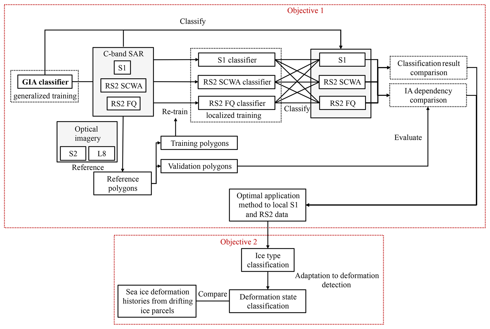
In summary, this study has two objectives: (1) to examine IA dependency of different ice types in S1 and RS2 data and evaluate the cross-platform transferability of training in the application of the GIA classifier and (2) to test to what extent sea ice classification based only on HH and HV backscatter intensities of C-band SAR data can be used to separate level from deformed ice.
2.1 Materials
The materials and methods of this study are summarized in a flowchart in Fig. 1. SAR data used in this study are mainly wide-swath RS2 and S1 data, i.e., RS2 SCWA and S1 EW (hereafter referred to as S1) data. The spatial resolution of these datasets is too coarse to detect individual leads and ridges less than approximately 100 m wide, but it is sufficient for isolating leads several hundred meters wide and separating areas dominated by deformed or level ice (Murashkin et al., 2018; Johansson et al., 2017). RS2 FQ data are also included to investigate the use of its higher spatial resolution to delineate ice deformation features. The analysis of SAR data focuses on the HH and HV channels, based on which the GIA classifier is trained.
Several datasets are used as reference to the derivation of training and validation polygons. Firstly, Sentinel-2 (S2, Level-2A bottom-of-atmosphere (BOA) reflectance) and Landsat-8 (L8, Level-2 atmospherically corrected surface reflectance) data with less than 50 % nominal cloud coverage are collected to provide optical reference. Secondly, back-tracking of sea ice source regions from ice drift fields derived from passive microwave data (Itkin et al., 2017), as well as in situ observations from the Norwegian young sea ICE 2015 (N-ICE2015) campaign, provides knowledge of the general distribution of ice types, especially first-year ice (FYI) and multi-year ice (MYI). Finally, the global sea ice type product from OSI SAF (10 km resolution), which provides separation between FYI and MYI using passive and active microwave scatterometers, is used as an additional reference (OSI SAF, 2015). No in situ data collected during N-ICE2015 are usable as a reference due to minimal spatial overlap with satellite data.
This study focuses on sea ice surrounding the N-ICE2015 expedition north of Svalbard at the western end of the Transpolar Drift (Granskog et al., 2017, 2018) to utilize expert knowledge from co-authors who participated in the campaign. Data collected during N-ICE2015 are used as the primary dataset, while SAR scenes with optical imagery overlap from 2016 to 2019 are also used to expand the dataset for retraining and validation. In situ observations show that sea ice investigated during N-ICE2015 primarily consisted of a mixture of FYI and second-year ice (SYI), while other thinner ice types including nilas and young ice also existed. SYI belongs to the MYI category in SAR-based sea ice classification and was the only type of MYI observed in the N-ICE2015 campaign. Frost flower coverage of young ice was observed for the entire N-ICE2015 drift (Itkin et al., 2017; Johansson et al., 2017; Granskog et al., 2017, 2018; Singha et al., 2020). This study mainly uses data covering the core of winter after freeze-up and before melt onset, i.e., January to April, as defined by Barber et al. (2001) based on time series evolution of C-band backscatter coefficients. This is to avoid the influence of wet snow on radar backscatter, which reduces radar penetration depth and result in dominant backscatter from the air–snow or dry–wet snow interface (e.g., Gill et al., 2015).
Specific selection procedures of satellite data are specified in Sect. 2.2, and the final list is summarized in Table 1 (Gatti and Bertolini, 2015; Northrop, 2015; (MDA), 2016, 2018). Image boundaries of RS2 SCWA and S1 scenes are shown in Fig. 2.
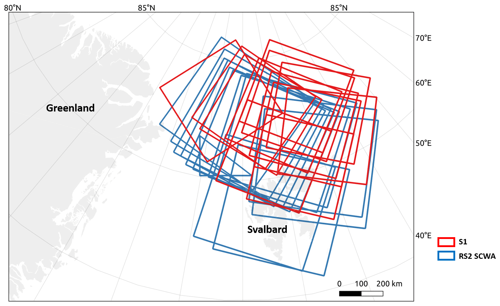
Figure 2Extents and overlaps of S1 and RS2 SCWA scenes used in this study.
The GIA classifier is used for sea ice classification to utilize its class-specific correction of IA dependency of SAR backscatter. This phenomenon is traditionally treated as an image property and remedied by a global correction based on the approximate linear decrease rate in the log domain (Zakhvatkina et al., 2019; Toyota et al., 2020). However, per-class IA correction is found to be necessary as the decrease rates (slopes of backscatter intensities vs. IA, i.e., IA slopes) are different for different surfaces (Gill et al., 2015; Liu et al., 2015; Mäkynen and Juha, 2017; Mahmud et al., 2018; Park et al., 2020). The GIA classifier directly incorporates IA dependency of classes into a Bayesian classifier (Theodoridis and Koutroumbas, 2008), which is achieved through the replacement of the constant mean vector of the Gaussian probability density function with a linearly variable mean. This shows significantly improved performance compared to classification with global IA correction. The terminology of sea ice classes used in this study is defined in Sect. 2.4.
2.2 Data selection and processing
The following selection and masking processes are conducted on RS2 scenes.
-
The original GIA classifier has limited separating capacity between open water and sea ice, as IA slopes and backscatter intensities of open water in different sea states vary significantly, creating ambiguities with ice surfaces (Lohse et al., 2020). To mitigate this known issue and also to serve our purpose of separating level from deformed ice within pack ice, daily sea ice concentration data generated from SSMI/S (Special Sensor Microwave Imager/Sounder, DMSP F18 satellite) from NSIDC (National Snow & Ice Data Center, Comiso, 2017) are used to filter out areas in RS2 SCWA scenes with ice concentration values lower than 87 %. This is an empirical threshold derived from visual inspection for the removal of large, contiguous open-water areas and the marginal ice zone.
-
The RS2 scenes are further selected based on the availability of overlapping S1 data and optical imagery. For 2015, RS2 scenes with at least one overlapping S1 scene are retained for analysis. From 2016 to 2019, RS2 scenes with at least one S1 and one optical (S2 or L8) scene with significant near-coincident overlap (overlapping area ≥30 % of the masked RS2 SCWA scene) are selected to ensure optical reference, resulting in only two RS2 SCWA scenes investigated in 2019 (Table 1). The maximum temporal separation between overlapping RS2 data and S1, S2 and L8 data is 1, 5.3 and 8 h, respectively. These selection parameters are empirically determined according to data availability. The overlap analysis is conducted through a script in Google Earth Engine (Gorelick et al., 2017), from which overlapping S1 scene IDs are derived and used for downloading using the Sentinelsat Python API (Marcel et al., 2021), while RGB composites of S2 and L8 data (bands 4, 3 and 2) are directly generated and downloaded.
Pre-processing of RS2 and S1 data is performed using the SNAP software package (European Space Agency, 2020). All scenes are radiometrically corrected and calibrated to σ0 values, so that RS2 and S1 backscatter is directly comparable. For RS2 FQ scenes which are single look, 2×2 multi-looking is performed to reduce speckle and reach a similar number of effective looks compared to the wide-swath scenes, while considering the preservation of linear features of interest, especially leads. Then, speckle filtering (boxcar, 3×3) is applied on all SAR scenes, and backscatter intensities are converted to decibels.
Typically several S1 scenes overlap with each RS SCWA scene, but the one with the largest overlapping area is selected to avoid redundancy. The first sub-swath of each S1 scene is removed for more reliable classification results, as radiometric variations are especially pronounced between the first sub-swath and others (e.g., Park et al., 2019). The identical masking process to remove pixels with low ice concentration is conducted on S1 scenes. No further processing is conducted on S2 and L8 RGB composites, as they are used qualitatively as reference data. Subsequent data analyses are performed using MATLAB (The Mathworks Inc., 2020) and Python (Van Rossum and Drake, 2009).
2.3 Cross-platform application of the GIA classifier
The original GIA classifier (Lohse et al., 2019) aims for Arctic-wide applicability and thus has been trained on S1 scenes spread across the Arctic region from 2015 to 2019, in “winter and early spring” months when ice is under freezing conditions (Lohse et al., 2020). Therefore, the class-specific IA dependencies in the classifier are produced from a generalized training set, and in theory encompass all IA dependencies of these classes within the spatial and temporal domain of that study. This study focuses on the transferability of training between S1 and RS2 data, for which we do not target Arctic-wide generalization. Instead, we focus on the N-ICE2015 region during boreal winter 2015 to provide confidence to the validity of training and validation with input of expert knowledge. Thus, we investigate the applicability of local training sets separately derived from S1 and RS2 scenes to both platforms, through which between-sensor differences in sea ice backscatter can be assessed.
For this purpose, reference polygons are derived for the SAR datasets based on visual examination of the scenes for retraining and validation. Polygons in the overlapping areas of corresponding RS2 SCWA and S1 scenes are used for both sensors, with manual adjustments accounting for their time difference (change of ice types in the polygons across different scenes due to sea ice drift). This study uses the ice classes in the original GIA classifier excluding open water, for reasons mentioned above. These classes are leads, young ice, level FYI (LFYI), deformed FYI (DFYI) and MYI (explained in more detail in Sect. 2.4). The criteria for selecting the polygons are as follows.
-
Size. Polygons of the same size within each dataset are used to standardize the number of pixels in each class: 300 m by 300 m for RS2 SCWA and S1 scenes and 30 m by 30 m for RS2 FQ scenes, which are approximately 3 times their effective pixel sizes given their number of looks. The choice of this size takes into account typical widths of linear features, mainly leads and young ice.
-
Distribution. A minimum distance of 30 pixels is kept between polygons to minimize spatial dependence between polygons of the same class. For each class, the polygons are distributed evenly across the entire range of IAs (where possible).
-
Numbers. In total 100 polygons are delineated for each scene, and the same number (20) of polygons are selected for each class (where possible). As the five classes are usually uneven in spatial coverage, probability sampling, e.g., spatially random or systematic sampling, is not used to avoid underrepresentation of scarcely occurring classes.
For classes usually with small spatial coverage (leads and young ice) where criteria 2 and 3 cannot both be satisfied (i.e., small spatial coverage leading to inevitable selection of polygons in small areas), criterion 3 is given priority to yield more polygons. Examples of reference polygons are shown in Fig. 3. Polygons shown in the SAR scenes are used in the analysis, while those in the optical scenes are manually shifted polygons which account for time differences from the SAR scenes and are therefore only for illustration purposes. Polygons in each scene are randomly split in half, with the number in each class also split in half, for retraining and validation. Training polygons for all S1 scenes are merged into an S1 training set, and those for RS2 SCWA scenes and FQ scenes are separately merged into RS2 SCWA and RS2 FQ training sets. Thus, for each dataset (S1, RS2 SCWA or RS2 FQ), retraining incorporates IA dependencies in all scenes. This is especially essential for RS2 FQ scenes where their small extent (spatial coverage: 25 km by 25 km; IA range: 1.24 to 1.94∘) necessitates the combined investigation of IA dependencies across multiple scenes.

Figure 3(a) Examples of reference polygons in different ice types in overlapping parts of SAR (false-color RGB composites: R:HV, G:HH, B:HH) and optical scenes and (b) examples of zoomed-in subsets for each class.
To evaluate cross-dataset transferability of training, the original GIA classifier is firstly applied to all datasets, providing a baseline for further analyses. Secondly, the regional training sets for S1, RS2 SCWA and RS2 FQ scenes are used to retrain the classifier and classify each dataset. Based on the evaluation of the results using validation polygons, the transferability of training is assessed, and the classification maps derived using the optimal classifier are selected to separate level from deformed ice.
2.4 Adaptation to separate level from deformed ice
To allow for direct comparison with ice deformation maps (see Sect. 2.5), the five-class classification scheme of the GIA classifier is altered to a three-class one: deformed ice, level ice and others, i.e., the classification of “deformation states.” The correspondence between the two schemes is as follows.
-
DFYI and MYI: deformed ice. An ideal classification of level and deformed ice requires separation between deformation states in every ice age category (mainly young ice, FYI and MYI). However, the GIA classifier does this only for FYI, such is common practice of SAR-based sea ice classification (e.g., see review by Zakhvatkina et al., 2019). Specifically, the DFYI class refers to rough FYI with stronger backscatter due to either ridging or the presence of other rough surface features, e.g., pancake ice.
MYI surface is usually rougher than younger ice types due to more accumulated deformation. The separation of MYI deformation states using SAR-based classification is challenging due to stronger presence of volume scattering from the desalinated and porous upper ice layer (increasing backscatter from level ice) as well as weathering of deformation features (decreasing backscatter from deformed ice; Dierking and Dall, 2007, 2008; Casey et al., 2014). As this study uses C-band HH and HV intensities only, this volume scattering component in MYI is significant, while the capacity of fully polarimetric data to distinguish between surface and volume scattering is not available (Moen et al., 2013; Casey et al., 2014). For the same reason, the contribution from volume scattering and ice deformation to strong SAR backscatter (characteristic of both DFYI and MYI) cannot be perfectly separated, creating ambiguities between DFYI and MYI. Thus, although MYI is not necessarily physically associated with ice deformation, this study groups MYI together with DFYI as “deformed ice.”
-
Young ice and LFYI: others. Among the many forms and stages of growth, the young ice class defined in the GIA classifier corresponds to rough young ice covered by frost flowers (mostly in re-frozen leads), i.e., fragile ice crystals typically 10–30 mm in height. The presence of frost flowers creates small-scale (millimeters to centimeters) surface roughness on the young ice surface, which has been shown to cause a C-band backscatter increase of 6–15 dB (Martin et al., 1995; Isleifson et al., 2010, 2018). The examination of SAR scenes used in this study shows that these young ice areas can reach similar backscatter intensities to MYI. It has been demonstrated that typical deformation in young ice, i.e., ice rafting, is difficult to distinguish using C-band SAR (Dierking, 2010) and therefore is not included in the analysis. Observations taken during N-ICE2015 show that rafting seldom occurred for young ice in the study area. Young ice was predominantly level with frost flower coverage, while ridging primarily occurred where young ice was close to thick ice. Example photographs of young ice from the campaign are shown in Fig. 4. Level young ice is not part of the five-class scheme, as the LFYI class does not exclude level ice less than 30 cm thick due to similar backscatter (Dierking and Dall, 2008; Dierking, 2010). As we are interested in ice deformation occurring on thicker ice, i.e., FYI and MYI, young ice is labeled “others” along with LFYI.
-
Leads. The leads class in the GIA classifier corresponds to ice openings occupied by calm open water, nilas or newly formed ice, thus having the lowest backscatter intensities. The separation between open water in different wind states is not within the scope of this study. As mentioned above, an ice concentration product is used to filter out large contiguous water bodies. The remaining water bodies all reside in leads that are away from the marginal ice zone and thus more sheltered from winds. Within the SAR scenes used in this study, visual examination shows that open water in all major leads is calm. This class is of direct interest in the second goal of this study and is labeled “leads” in the three-class scheme.
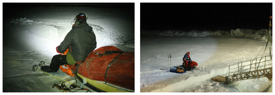
Figure 4Example photographs of young ice witnessed in the N-ICE2015 campaign within the study area (photos: P. Itkin).
2.5 Deformation parcel tracking
Six pairs of S1 scenes from 21 to 26 January 2015 (one image pair per day) surrounding the N-ICE2015 region are used to construct ice deformation history for drifting ice parcels based on the sea ice drift algorithm developed by Korosov and Rampal (2017). Sea ice deformation is calculated from line integrals as described in, for example, Bouillon and Rampal (2015) and Itkin et al. (2017) and further filtered for noise. Sea ice drift is calculated on a 400 m regularly spaced grid and deformation on the corresponding triangular grid. The deformation states are classified as no deformation, divergence and convergence. The rectangular parcels are initiated on the first day of the image sequence on a regular grid with centroids spaced by 300 m at a size of 120 km by 120 km. Initially, all parcels are undeformed. For each subsequent day the parcels move with the average velocity of the drift calculated within a 300 m radius of each parcel centroid. At every step, each ice parcel accumulates counts of each deformation class based on the average value inside the 150 m radius from the centroid. Finally, based on the total number of counts, every parcel is classified into undeformed, predominantly convergence, predominantly divergence or a mix of both. These Lagrangian parcel products are then gridded onto a 100 m grid based on the nearest-neighbor value. In the 6 d of parcel tracking, the ice pack undergoes episodic deformation limited to several active linear kinematic features (LKFs). The effects of this recent deformation can then be visually compared with the classification results, thus examining the ability of the classification to recognize the most recently formed ice deformation features.
3.1 Cross-platform application of the GIA classifier
3.1.1 Classification accuracy and qualitative comparisons
The classification accuracies (CAs; Fig. 5) show that for all datasets regional retraining leads to similar and significant improvements in classification performance over the original GIA classifier. Firstly, regional training sets (Fig. 5a–c, columns S1, RS2 SCWA and RS2 FQ) yield average CAs significantly higher than the original GIA classifier (Fig. 5a–c, columns O), which is expected as regional validation is used. Secondly, within each dataset, regional training sets yield similar overall CAs, despite the “corresponding” training sets (Fig. 5a column S1, b column RS2 SCWA and c column RS2 FQ), yielding higher average CAs (87.63 %, 89.31 % and 91.70 %) than the rest (p values shown in Fig. 5). This corresponds well with our expectation of similar sea ice backscatter (σ0) for the two C-band sensors, while suggesting dataset-specific retraining can be used to achieve optimal overall accuracies.
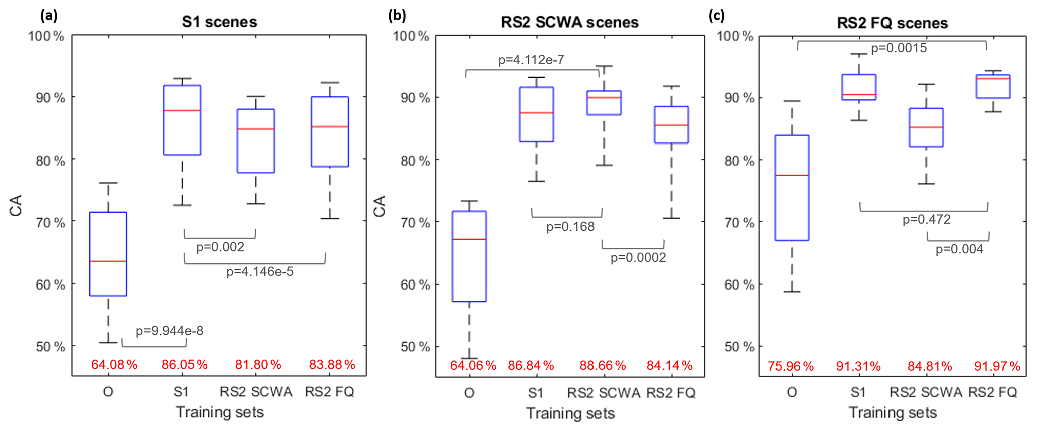
Figure 5CAs for S1, RS2 SCWA and RS2 FQ scenes using the original and retrained GIA classifier. O: training for the original GIA classifier; S1, RS2 SCWA, RS2 FQ: regional S1, RS2 SCWA and RS2 FQ training, respectively. Mean CAs are displayed in red below the box plots. P values of the difference in mean CAs are also shown.
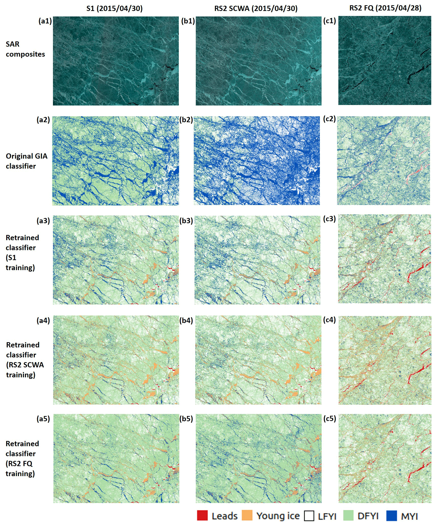
Figure 6Example comparisons between classification results using the GIA classifier with different training.
Examples of qualitative comparison between results using the GIA classifier with different training are shown in Fig. 6. The original GIA classifier yields classification maps dominated by DFYI (green) and MYI (blue), while visual inspection of the SAR RGB composites (Fig. 6a1–c1) indicates significantly more prominent existence of LFYI, rough young ice and leads. This is caused by frequent misclassification of young ice as MYI and leads as LFYI. The three underrepresented ice types (LFYI, rough young ice and leads) are better recognized by the regionally retrained GIA classifier for all datasets (Fig. 6a3–c3, a4–c4, a5–c5). This shows the expected improvement of classification performance from regional retraining as evaluated by regional validation. The GIA classifier with different regional training (Fig. 6a3–c3 vs. a4–c4 vs. a5–c5) yields results with similar spatial distribution of ice types.
3.1.2 IA dependencies
Theoretically, the performance of cross-dataset application of training is driven by the different IA dependencies of the ice types they record. To investigate this, scatter plots of HH intensities and IAs for different ice types are derived using the validation polygons (Fig. 7). NESZ values across the IAs are plotted for comparison. Corresponding least-squares linear regression lines are also plotted. HH–IA slopes derived from validation polygons as well as the original and retrained (using corresponding training sets) GIA classifier are summarized in Table 2, with slope values from previous studies using winter C-band satellite SAR data listed for reference. For all datasets, the HV signals show less IA dependency and are much more affected by noise, but their inclusion in the classifier has been demonstrated to improve class separations (Lohse et al., 2020). For our study area, the difference in HV–IA dependencies provides additional separating capability between MYI and young ice, while those for leads, LFYI and DFYI are severely influenced by noise floor configurations. Otherwise, the analysis of HV–IA dependencies provides little additional information relating to our objectives and is not shown here.

Figure 7HH–IA scatter plots, least-squares regression lines for different ice types and NESZ values for different datasets.
Table 2HH–IA slopes () of different ice types derived in this and previous studies (SCN: ScanSAR Narrow; ASAR WS: Advanced Synthetic Aperture Radar, Wide Swath; QEI: Queen Elizabeth Islands). Slope values in previous studies are presented in their original forms.
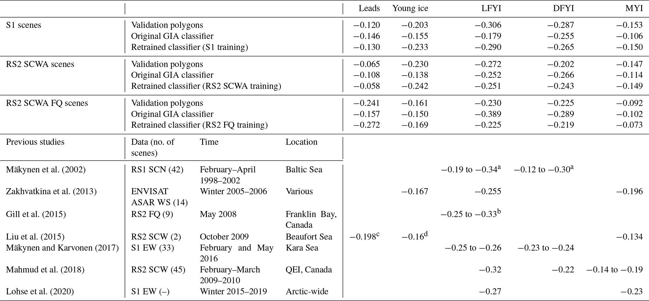
a Slopes of FYI with dry snow on top.
b Slopes of land-fast smooth FYI with thin (7.7±3.9 cm) to thick (36.4±12.3 cm) snow cover.
c Slope of nilas.
d Slope of deformed gray ice.
The original GIA classifier (Fig. 7a2–c2) yields similar separation between ice types across datasets, showing the characteristics of its generalized S1 training. Comparatively, the validation polygons yield different class separations (Fig. 7a1–c1) representing the local condition in the study area. The class separations and IA slopes of ice types from regional training are reflected in the retrained classification results (Fig. 7a3–c3, a4–c4, a5–c5). The training set corresponding to each dataset (Fig. 7a3, b4 and c5) produces class separation most similar to the validation polygons.
The comparative class separations and IA slopes from different training sets explain the above qualitative comparisons (Sect. 3.1.1): (1) the generalized training shows flatter HH–IA slopes and lower-extending HH values for LFYI, which results in its strong overlap with leads (Fig. 7a2–c2), while the regional training sets yield steeper slopes for LFYI (Fig. 7a1–c1), resulting in better separation between the two classes; (2) young ice and MYI are shown in all training sets to have similar HH intensities (Fig. 7a1–c1), but they show better separation in the HV channel for the regional training sets than the generalized one (not shown).
HH–IA slopes of different ice types are within the range of values reported by previous findings (Table 2), having considered that they are derived from different areas across the Arctic region. Comparative IA slopes for different ice types also conform to the literature: (1) IA slopes of DFYI are less than those of LFYI, as deformation features are strong scatterers which lead to higher standard deviation in backscatter intensities in small (local) IA intervals, and this added randomness in backscatter is not sensitive to IA; (2) compared to FYI, MYI has lower IA slopes due to the sensitivity of C-band radar signal to air bubbles in MYI, leading to substantial presence of volume scattering (when compared to SAR sensors at longer wavelengths, e.g., L-band), which is less sensitive to IA (Mäkynen et al., 2002; Dierking and Dall, 2007; Mahmud et al., 2018; Zakhvatkina et al., 2013; Mäkynen and Juha, 2017; Lohse et al., 2020). For each dataset, when compared to the original GIA classifier, the classifier retrained using the corresponding training set yields slope values closer to the validation polygons.
3.1.3 Leads and noise floors
Between the two wide-swath datasets (S1 EW and RS2 SCWA), the IA slopes for young ice, FYI and MYI follow similar trends (Fig. 7, columns a and b). However, the IA slope for leads in the RS2 SCWA training is visibly flatter than that in the S1 training, which is confirmed by their respective slope values in Table 2 (−0.12 for S1 and −0.065 for RS2 SCWA). The plotted NESZs show that leads for S1 scenes are above the noise floor throughout the IA range (Fig. 7b1), while for RS2 SCWA scenes (with a flatter noise floor), it is very close to and reaches the noise floor at an approximate IA of 30∘ (Fig. 7b2). This explains the flatter IA slope for leads in RS2 SCWA scenes.
For the RS2 FQ scenes, IA slopes for the young ice, FYI and MYI (Fig. 7c1) are similar to the wide-swath datasets. The RS2 FQ scenes are well within pack ice, and the leads that these scenes additionally recognize due to higher spatial resolution (compared to wide-swath scenes) are very narrow and scarce. Therefore, the multi-looking and speckle filtering processes have mixed the pixel values in narrower leads to surrounding pixels with higher backscatter intensities, resulting in small numbers of reference polygons. This has prevented full evaluation of its IA dependency due to uneven representation across IAs. However, the existing reference polygons show that HH intensities of RS2 FQ lead pixels do not reach the noise floor across the IA range and therefore do not present the above issue in the RS2 SCWA training.
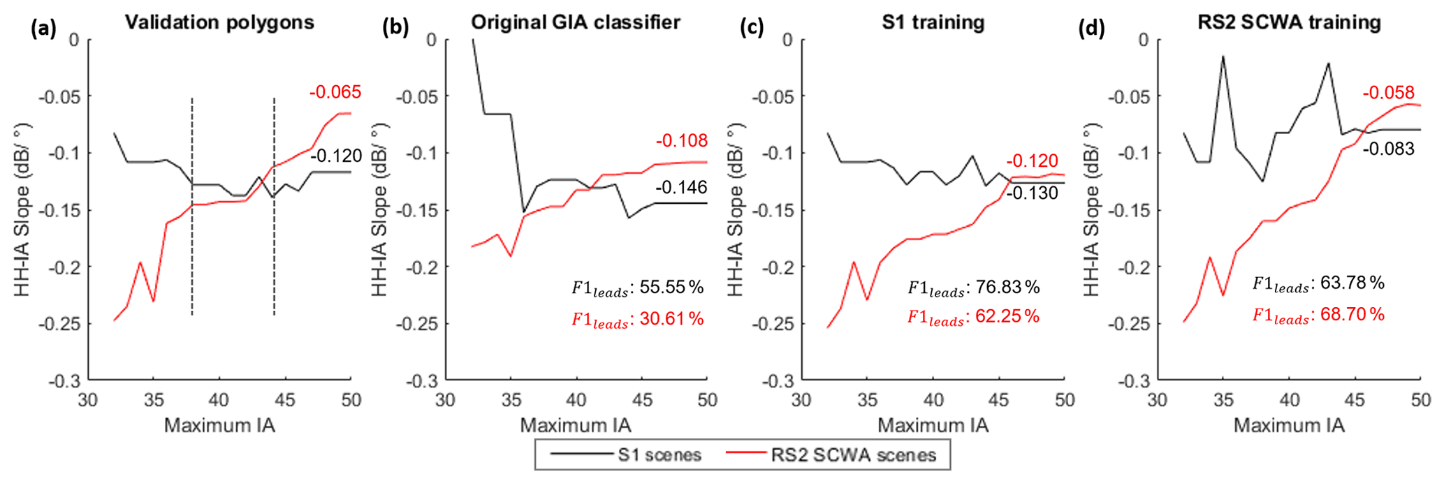
Figure 8HH–IA slopes for different IA maximums and F1 scores of the leads class, with the overall slopes (maximum IA = 50) shown in corresponding colors (black: S1 scenes; red: RS2 SCWA scenes).
To further investigate the interaction between leads and respective noise floors of the sensors, IA slopes for leads from the near range to increasing IA maximums are plotted in Fig. 8. F1 scores (Chinchor, 1992) of the leads class, which combines producer's and user's accuracies, and are shown to evaluate the overall accuracies of this class. S1 validation polygons show relatively constant HH–IA slopes across the range of IA maximums (Fig. 8a, black lines). For RS2 SCWA scenes (Fig. 8a, red lines), the slopes are steeper (higher absolute values) for IA maximums in the near range and stabilize after reaching a similar slope level to S1 scenes (approximately −0.16 to −0.12 , at IA maximums from 38 to 44∘, as shown between the dashed lines). The slopes then quickly flatten (lower absolute values) as the IA maximum approaches the far range, eventually reaching a much flatter overall slope of −0.065 compared to −0.120 for S1 scenes. This confirms the findings from Fig. 7a2 where the lead pixels reach the noise floor at approximately 30∘, and remain at a similar decibels level due to the noise floor. Thus, using the S1 training on RS2 SCWA scenes will inevitably introduce incorrect IA dependency for leads, leading to misclassification and vice versa. It then follows that for a specific lead in a SAR scene, its spatial coverage in the range direction, influenced by its positioning, length and orientation, will impact the degree of this misclassification of pixels inside.
For the classification results (Fig. 8b–d), the training used by the original GIA classifier yields different overall IA slopes than the regional validation for leads in both datasets, resulting in relatively low classification accuracies, as shown by the F1 scores (Fig. 8b, F1leads). When applied to their corresponding datasets, the regional S1 and RS2 SCWA training sets (Fig. 8c, black; Fig. 8d, red) yield HH–IA slopes across IA maximums similar to their respective validation polygons (Fig. 8a). Comparatively, cross-platform application of training sets (Fig. 8c, red; Fig. 8d, black) produces lower accuracies, confirming the findings above.
To inspect this effect in classification maps, an example classification of an RS2 SCWA scene is given in Fig. 9, which shows the difference between different training in recognizing leads in different IA ranges. For the near range, the GIA classifier with S1 and RS2 SCWA regional retraining (Fig. 9c1 and d1) yields very similar spatial coverage of leads. In IAs between 34 and 39∘, classification using the RS2 SCWA training (Fig. 9d2) produces a more complete representation of the leads than the S1 training (Fig. 9c2) where parts of the leads are identified as LFYI. In IAs between 40 and 45∘, the RS2 SCWA training preserves all visible leads (Fig. 9d3) while the S1 training keeps only part of the main ice opening (Fig. 9c3, circled in black) but almost entirely misses the other leads. This gradual increase in misclassification of leads as LFYI with IA corresponds well with Fig. 7 (column b): the stronger HH–IA dependency for leads in S1 training (steeper IA slopes than RS2 SCWA training) yields the same lead–LFYI separation in the near range but shows gradually more misclassification of leads to LFYI (Fig. 7b3 compared to b4) in IAs greater than approximately 37∘. The same is true for RS2 SCWA training when used to classify S1 scenes (Fig. 7a4 compared to a3), where its flatter HH–IA slope leads to misclassification of LFYI to leads in the far range.
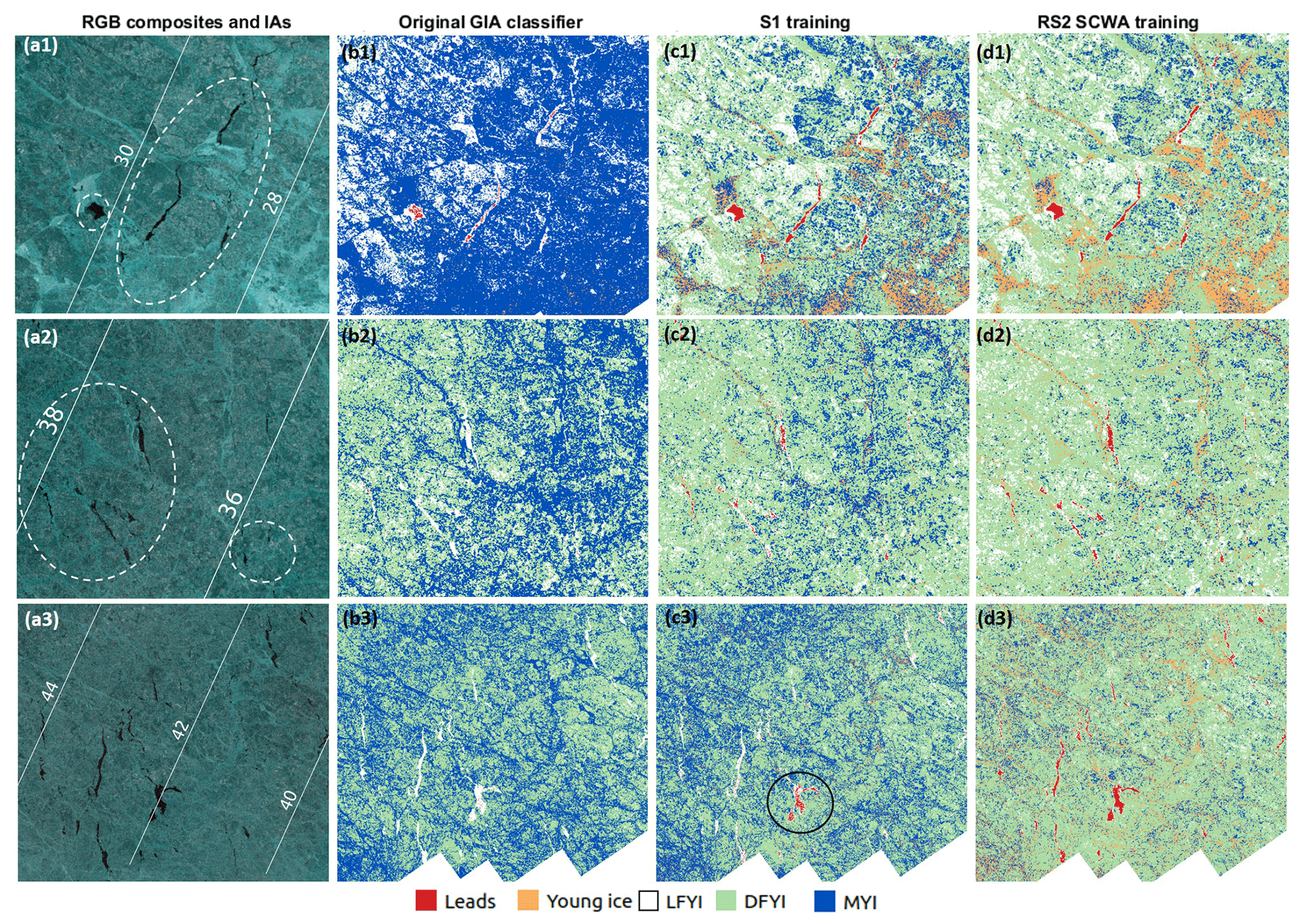
Figure 9Comparison of classification results in different IA ranges for the RS2 SCWA scene on 5 March 2015, where IA contours with values are shown in white, and main areas containing the leads class are circled in white in (a1–a3).
From the above analyses of CAs, HH–IA dependencies and qualitative comparisons, it can be concluded that in our study area, S1 and RS2 SCWA training sets are transferable with the exception of the leads class. This is caused by the different interactions between backscatter from leads and the noise floors in the two datasets, i.e., the flattened IA slope of leads in RS2 SCWA data due to contact with the higher noise floor. This means that between wide-swath S1 and RS2 data, transfer learning can only be conducted on classes other than leads for whole scenes or on all classes in the near range. Otherwise, retraining is needed for reliable separation between leads and LFYI. The RS2 FQ scenes yield similar IA slopes for classes other than leads compared to the wide-swath datasets, while full assessment of leads is impeded by the lack of reference polygons. Retraining to the study area also increases performance of the GIA classifier when applied to S1 scenes. Based on these assessments, the S1, RS2 SCWA and FQ scenes are classified using the GIA classifier regionally retrained using their corresponding training sets and are used for the following comparison to ice deformation.
3.2 Comparison between classification results and deformation parcels
The five classes in the classification results are summarized into three deformation states and compared with the deformation parcels (Fig. 10). During the period of ice parcel tracking (21–26 January 2015), a storm with a peak wind speed of 10.8 m s−1 passed through Fram Strait (storm M1, 21 to 22 January; Cohen et al., 2017) and hit the area surrounding the N-ICE2015 research camp (Cohen et al., 2017; Graham et al., 2019). The storm first pushed ice northward, compacting the ice pack and causing ice deformation along re-frozen leads and cracking thicker ice floes. It then transported ice southward towards the ice edge in the second phase, generating strong divergence and opening along the same leads and cracks. Following the storm passage, newly opened leads rapidly re-froze following the returning of dry and cold conditions, creating new ice (Itkin et al., 2017; Graham et al., 2019). Accordingly, the parcels (Fig. 10, row e) indicate major presence of new and deformed ice concentrated along several LKFs. Divergence zones with new lead ice prevail but are mixed with convergence zones where deformed ice is expected to be produced, mainly in the middle of the maps (Fig. 10e1 and e3). The northeastern and southern parts of the maps experienced mainly ice divergence, marked by solid ellipses.
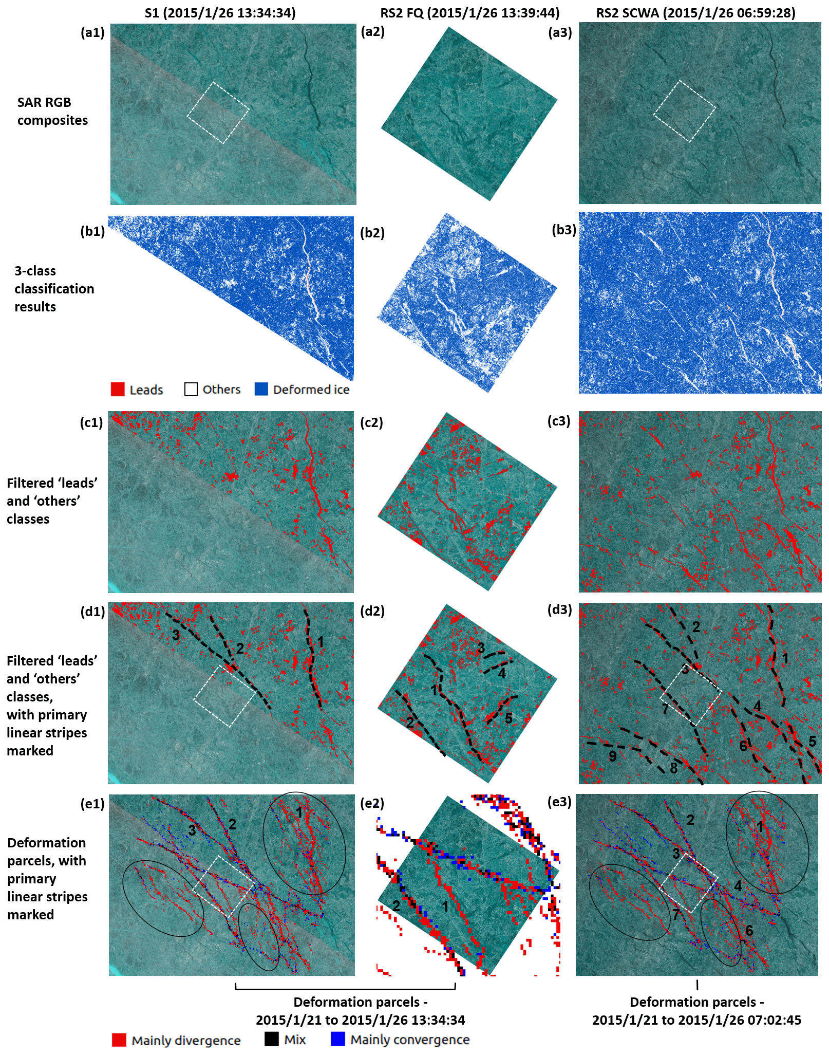
Figure 10Comparison of classification results and deformation parcels. Classification results (b1–b3) are derived using the GIA classifier retrained using corresponding training sets. The position of the RS2 FQ scene is shown as white rectangles in the wide-swath scenes (a1, a3).
It is difficult to interpret direct correspondence between the deformation parcels and the classification maps, as areas of ice divergence and convergence do not directly correspond to specific ice types, and the deformation parcel maps only represent ice motion accumulated in the 6 d period. Still, observations can be made for (1) whether the classified ice types correctly correspond to ice divergence or convergence indicated by the deformation parcels and (2) whether the classification maps and deformation parcels each identify visible deformation features not shown by the other.
-
Classification results. An overall examination of classification maps (Fig. 10b1–b3) shows that deformed ice is pervasive. The same can be concluded from visual examination of the SAR RGB composites (Fig. 10a) and is reported by N-ICE2015 records and observations (Itkin et al., 2017; Granskog et al., 2018; Graham et al., 2019). However, the true percentage of deformation in the scene cannot be retrieved or confirmed using available data. This is due to the inclusion of ice surface with other rough surface features in the DFYI class, as well as ambiguity between DFYI and MYI, as mentioned above. The deformed ice class (three-class scheme) is comprised of mainly DFYI (five-class scheme).
On the other hand, many LKFs in the others and leads class (three-class scheme) are visible in the classification maps (white in Fig. 10b1–b3). These are comprised of mostly LFYI in re-frozen leads (five-class scheme), which can physically correspond to smooth young ice or FYI, as mentioned above. To more clearly examine the correspondence of the leads and others classes to the deformation parcels, pixels in these classes are extracted, from which small, disconnected pixel groups (<100 pixels for wide-swath scenes and <500 pixels for the RS2 FQ scene) are removed. These filtered pixels (Fig. 10c1–c3, in red) clearly show the abovementioned LFKs, with the primary ones marked by dashed lines and numbered in Fig. 10d1–d3. Most of these level ice areas also appear in the deformation parcel maps (Fig. 10e1–e3), where they are numbered accordingly. Lines 5, 8 and 9 in Fig. 10d3 do not appear in the deformation parcel maps (Fig. 10e3) as they are out of the maps' areal coverage. Open-water areas in line 1 in Fig. 10b1 and b3 are correctly classified as leads (in red). The RS2 FQ scene shows similar distribution of ice types, but its higher spatial resolution picks up some more visible ice openings with more spatial details (lines 1, 3, 4 and 5 in Fig. 10d2) compared to d3).
-
Deformation parcels. For the deformation parcels, the most prominent (widest) features have more recognizable correspondence to features delineated by the classifications. These are either mostly ice divergence mixed with convergence or exclusively divergence. For example, the end states of lines 2 and 3 in Fig. 10e1 and e3 are dominated by LFYI and young ice, surrounded by DFYI (not shown), corresponding well to the co-authors' field experience of deformation occurrence at the interface between young ice and older ice. The pixels showing “mostly convergence” are derived from values accumulated in the 6 d period and therefore cannot represent deformation accumulated over longer periods. The abovementioned areas indicating mainly ice divergence (Fig. 10e1 and e3, solid ellipses, excluding the major lead, i.e., line 1) are less recognizable in the classification maps. Five-class classifications indicate these are narrower and smaller leads occupied mostly by LFYI and young ice. Areas in which deformation parcels indicate prominent presence of ice convergence are mainly classified as the deformed ice class, interrupted by small areas of others.
The areal fraction of deformation parcels occupied by each class is shown in Fig. 11. Due to the coarse resolution of the deformation parcels compared to the SAR scenes, the contrast between parcels of mainly convergence and “mainly divergence” in terms of the comparative proportions of deformed ice and others is not prominent. Nevertheless, the fractions of the leads and others classes in areas of ice divergence are higher than in those of ice convergence, corresponding well with the above findings. For the same reason regarding spatial resolution, a large fraction of the parcels are classified as deformed ice, which is the dominant class in areal coverage in the SAR scenes. The others class takes up 22.13 % to 34.38 % of all types of deformation parcels, indicating that on average, approximately a quarter of a deformation parcel pixel (a 300 m × 300 m area) is comprised of others. This matches typical widths of deformation features in the study area and period.

Figure 11Areal fractions of different classes (three-class scheme) within deformation parcel pixels.
To summarize, the classifications capture ice openings in the leads and others classes that correspond well with areas of ice divergence. This good correspondence is also partly due to the surface features created by ice divergence being more spatially confined. On the other hand, the deformed ice class includes a mix of DFYI and MYI that is spatially widespread, where the true proportions of deformed ice cannot be reliably verified and hence has limited correspondence with areas of ice convergence. This is due to both the accumulation of ice deformation in a period longer than the parcel tracking and also the limitation of the classifier working only with HH and HV channels of C-band sensors. Classification on the RS2 FQ scenes performs similarly to the wide-swath scenes but can serve to preserve more spatial details of surface features. The capacity of the classification results to identify these surface features (mainly ice divergence) in the deformation parcels serves as another validation of the regionally retrained GIA classifier.
3.3 Limitations and future steps
This study is a first step towards the goal of Arctic-wide ice deformation detection based on a consistent classification method applicable to multiple SAR platforms and thus investigates the cross-platform application of the GIA classifier in a regional setting. We work within the limitations of both the classifier and the characteristics of HH and HV channels of S1 and RS2, which affects the separation of level from deformed ice, as summarized above. Very limited ground truth of ice types from in situ data are available for retraining and validation, hence the heavy preference given to the N-ICE2015 dataset to utilize the co-authors' expert knowledge on ice conditions.
This study expands the application of the GIA classifier from S1 to RS2 data. Additional studies will be conducted, seeking further expansion of its application to more SAR platforms, e.g., X- and L-band SAR, which provides potential for better separation between ambiguous class pairs. IA dependency in SAR data with these different frequencies needs to be rigorously examined and validated. It is expected that frequency- and region-specific retraining will still be essential for deformation detection using the altered classifier, as SAR intensity contrast between level and deformed ice is sensitive to SAR properties as well as ice properties that vary across regions, e.g., small-scale roughness and ice volume structure (Dierking and Dall, 2007). The inclusion of more features into the classification is also desirable, e.g., polarimetric features sensitive to sea ice deformation (e.g., Ressel et al., 2016; Park et al., 2019), and also texture features (e.g., Park et al., 2020; Lohse et al., 2021). For example, the recent study by Lohse et al. (2021) investigated the IA dependencies of common texture features and demonstrated that incorporating these features into ice type classification can improve the separation of young ice and MYI, as well as the classification of open-water areas. However, the improvement comes at the cost of reduced spatial resolution due to the applied texture windows. Further integration of IA dependency into classifiers other than the Bayesian classifier is also desirable to seek better classification performances. Finally, successful cross-platform application of an optimal classification method can be used to create a reliable time series of classification maps, which can be better used to derive or compare with ice deformation products.
This study demonstrates that in our study area, S1 and RS2 data produce similar IA dependencies of different ice types, except the leads class due its interactions with different noise floors of the two sensors. Accordingly, based on the GIA classifier, our results have demonstrated that the direct transfer of training between the two platforms is applicable with the exception of leads. Dataset- and region-specific retraining is found to provide optimal classification performances, and the GIA classifier retrained specific to S1, RS2 SCWA and RS2 FQ datasets produces similar and improved classification results compared to the original classifier. The cross-platform application of the GIA classifier extends usable C-band SAR data over the study area from 2015 to present (S1) to 2010 to present (RS2). This study further provides reference to future cross-platform application of training between S1 and RS2, so valuable training sets can be better utilized, e.g., with proper retraining, or direct application in the near range or when leads are not of interest.
The comparison between deformation parcels and classification results with dataset-specific regional retraining shows the best correspondence in leads with open water and nilas, young ice, or LFYI, as prominent ice openings created by divergence following the storm passage are in linear forms and well captured by both analyses. The DFYI and MYI classes in the classification results do not clearly correspond to linear ice convergence zones indicated by deformation parcels, due to both the limitation of the classification method and the difference in the period of deformation accumulation. RS2 FQ scenes can be used to provide more spatial details in delineating deformation features. The comparison with deformation parcels further serves to partially validate the classification results.
In summary, through the cross-platform application of the GIA classifier, this study demonstrates the potential and obstacles in the transfer of training between S1 and RS2 data, as well as in the use of the classification to separate level from deformed ice. We expect future development of the classifier and the inclusion of additional datasets will enable the possibility of large-scale monitoring of ice deformation merely from the classification of widely available satellite SAR data.
The processing of SAR images was achieved using the open-source software SNAP provided by the European Space Agency (ESA) at https://step.esa.int/main/toolboxes/snap/ (last access: January 2021).
RADARSAT-2 data used in this study are not publicly available and were provided by NSC/KSAT under the Norwegian–Canadian RADARSAT agreement (2015 and 2019). Sentinel-1 and Sentinel-2 data are publicly available from the Copernicus Open Access Hub (https://scihub.copernicus.eu/, last access: January 2021; European Space Agency, 2015). Landsat 8 images are publicly available from EarthExplorer developed by the U.S. Geological Survey (2015) (https://earthexplorer.usgs.gov/, last access: January 2021). The OSI SAF global sea ice type product (OSI-403-d) is publicly available from https://osi-saf.eumetsat.int/products/osi-403-d (last access: January 2021; OSI SAF, 2015.
PI acquired funding for this study. PI, MJ and APD were involved in project administration and supervision. All co-authors were involved in the conceptualization of the study. WG was responsible for data curation, methodology design, formal analysis and result visualization. JL provided his codes and knowledge of the GIA classifier. PI produced the deformation parcel maps for comparison with the classification results. WG prepared the manuscript, with contributions from all co-authors in reviewing and editing.
The contact author has declared that neither they nor their co-authors have any competing interests.
Publisher's note: Copernicus Publications remains neutral with regard to jurisdictional claims in published maps and institutional affiliations.
The N-ICE2015 expedition was supported by the Centre of Ice, Climate and Ecosystems (ICE), Norwegian Polar Institute, Tromsø, Norway. The authors also extend their thanks to all who participated in the N-ICE2015 campaign, including personnel from the Norwegian Polar Institute, as well as many partner organizations and the R/V Lance crew. They would like to thank the personnel from UiT The Arctic University of Norway and the Norwegian Polar Institute, who made the co-located satellite image acquisitions possible, and Max König from NPI and Thomas Kræmer and Malin Johansson from UiT.
This research has been supported by the Norges Forskningsråd (grant nos. 287871, 237906 and 280616).
This paper was edited by Petra Heil and reviewed by two anonymous referees.
Arntsen, A. E., Song, A. J., Perovich, D. K., and Richter-Menge, J. A.: Observations of the summer breakup of an Arctic sea ice cover, Geophys. Res. Lett., 42, 8057–8063, https://doi.org/10.1002/2015GL065224, 2015. a
Asplin, M. G., Galley, R., Barber, D. G., and Prinsenberg, S.: Fracture of summer perennial sea ice by ocean swell as a result of Arctic storms, J. Geophys. Res.-Oceans, 117, 1–12, https://doi.org/10.1029/2011JC007221, 2012. a
Assmy, P., Fernández-Méndez, M., Duarte, P., Meyer, A., Randelhoff, A., Mundy, C. J., Olsen, L. M., Kauko, H. M., Bailey, A., Chierici, M., Cohen, L., Doulgeris, A. P., Ehn, J. K., Fransson, A., Gerland, S., Hop, H., Hudson, S. R., Hughes, N., Itkin, P., Johnsen, G., King, J. A., Koch, B. P., Koenig, Z., Kwasniewski, S., Laney, S. R., Nicolaus, M., Pavlov, A. K., Polashenski, C. M., Provost, C., Rösel, A., Sandbu, M., Spreen, G., Smedsrud, L. H., Sundfjord, A., Taskjelle, T., Tatarek, A., Wiktor, J., Wagner, P. M., Wold, A., Steen, H., and Granskog, M. A.: Leads in Arctic pack ice enable early phytoplankton blooms below snow-covered sea ice, Sci. Rep.-UK, 7, 1–9, https://doi.org/10.1038/srep40850, 2017. a
Barber, D. G., Hanesiak, J. M., and Yackel, J. J.: Sea ice, radarsat-1 and arctic climate processes: A review and update, Can. J. Remote Sens., 27, 51–61, https://doi.org/10.1080/07038992.2001.10854919, 2001. a
Bouillon, S. and Rampal, P.: On producing sea ice deformation data sets from SAR-derived sea ice motion, The Cryosphere, 9, 663–673, https://doi.org/10.5194/tc-9-663-2015, 2015. a, b
Cafarella, S. M., Scharien, R., Geldsetzer, T., Howell, S., Haas, C., Segal, R., and Nasonova, S.: Estimation of Level and Deformed First-Year Sea Ice Surface Roughness in the Canadian Arctic Archipelago from C- and L-Band Synthetic Aperture Radar, Can. J. Remote Sens., 45, 457–475, https://doi.org/10.1080/07038992.2019.1647102, 2019. a
Casey, J. A., Beckers, J., Busche, T., and Haas, C.: Towards the retrieval of multi-year sea ice thickness and deformation state from polarimetric C- and X-band SAR observations, in: International Geoscience and Remote Sensing Symposium (IGARSS), IEEE, 1190–1193, https://doi.org/10.1109/IGARSS.2014.6946644, 2014. a, b, c
Cavalieri, D. J., Markus, T., Ivanoff, A., Liu, A. K., and Zhao, Y.: AMSR-E/Aqua Daily L3 6.25 km Sea Ice Drift Polar Grids, Version 1, NASA National Snow and Ice Data Center Distributed Active Archive Center, Boulder, Colorado USA, https://doi.org/10.5067/AMSR-E/AE_SID.001, 2011. a
Chinchor, N.: MUC-4 Evaluation Metrics, in: Proceedings of the 4th Conference on Message Understanding, Association for Computational Linguistics, USA, McLean Virginia, USA, 16–18 June 1992, 22–29, https://doi.org/10.3115/1072064.1072067, 1992. a
Cohen, L., Hudson, S. R., Walden, V. P., Graham, R. M., and Granskog, M. A.: Meteorological conditions in a thinner Arctic sea ice regime from winter to summer during the Norwegian Young sea ice expedition (N-ICE2015), J. Geophys. Res., 122, 7235–7259, https://doi.org/10.1002/2016JD026034, 2017. a, b
Cole, S. T., Toole, J. M., Lele, R., Timmermans, M. L., Gallaher, S. G., Stanton, T. P., Shaw, W. J., Hwang, B., Maksym, T., Wilkinson, J. P., Ortiz, M., Graber, H., Rainville, L., Petty, A. A., Farrell, S. L., Richter-Menge, J. A., and Haas, C.: Ice and ocean velocity in the Arctic marginal ice zone: Ice roughness and momentum transfer, Elementa, 5, 55, https://doi.org/10.1525/elementa.241, 2017. a
Comiso, J. C.: Bootstrap Sea Ice Concentrations from Nimbus-7 SMMR and DMSP SSM/I-SSMIS, Version 3, NASA National Snow and Ice Data Center Distributed Active Archive Center, Boulder, Colorado USA, https://doi.org/10.5067/7Q8HCCWS4I0R, 2017. a
Dabboor, M., Montpetit, B., Howell, S., and Haas, C.: Improving sea ice characterization in dry ice winter conditions using polarimetric parameters from C- and L-Band SAR data, Remote Sens.-Basel, 9, 6859–6873, https://doi.org/10.3390/rs9121270, 2017. a
Dierking, W.: Mapping of Different Sea Ice Regimes Using Images From Sentinel-1 and ALOS Synthetic Aperture Radar, IEEE T. Geosci. Remote, 48, 1045–1058, https://doi.org/10.1109/TGRS.2009.2031806, 2010. a, b
Dierking, W. and Dall, J.: Sea-ice deformation state from synthetic aperture radar imagery – Part I: Comparison of C- and L-B and and different polarization, IEEE T. Geosci. Remote, 45, 3610–3621, https://doi.org/10.1109/TGRS.2007.903711, 2007. a, b, c
Dierking, W. and Dall, J.: Sea ice deformation state from synthetic aperture radar imagery – Part II: Effects of spatial resolution and noise level, IEEE T. Geosci. Remote, 46, 2197–2207, https://doi.org/10.1109/TGRS.2008.917267, 2008. a, b
Dybkjaer, G.: Medium Resolution Sea Ice Drift Product User Manual, Tech. rep., The Ocean & Sea Ice Satellite Application Facility (OSI SAF), 2018. a
European Space Agency: Copernicus Sentinel data, European Space Agency [data set], available at: https://scihub.copernicus.eu/ (last access: January 2021), 2015. a
European Space Agency: SNAP – ESA Sentinel Application Platform v7.0.4, available at: http://step.esa.int (last access: January 2021), 2020. a
Fernández-Méndez, M., Olsen, L. M., Kauko, H. M., Meyer, A., Rösel, A., Merkouriadi, I., Mundy, C. J., Ehn, J. K., Johansson, A. M., Wagner, P. M., Ervik, Å., Sorrell, B. K., Duarte, P., Wold, A., Hop, H., and Assmy, P.: Algal hot spots in a changing Arctic Ocean: Sea-ice ridges and the snow-ice interface, Frontiers in Marine Science, 5, 75, https://doi.org/10.3389/fmars.2018.00075, 2018. a
Gatti, A. and Bertolini, A.: Sentinel-2 Products Specification Document, S2-PDGS-TAS-DI-PSD, Thales Alenia Space, France, 13.1, 2015. a
Gegiuc, A., Similä, M., Karvonen, J., Lensu, M., Mäkynen, M., and Vainio, J.: Estimation of degree of sea ice ridging based on dual-polarized C-band SAR data, The Cryosphere, 12, 343–364, https://doi.org/10.5194/tc-12-343-2018, 2018. a
Gill, J. P. S., Yackel, J. J., Geldsetzer, T., and Fuller, M. C.: Sensitivity of C-band synthetic aperture radar polarimetric parameters to snow thickness over landfast smooth first-year sea ice, Remote Sens. Environ., 166, 34–49, https://doi.org/10.1016/j.rse.2015.06.005, 2015. a, b
Gorelick, N., Hancher, M., Dixon, M., Ilyushchenko, S., Thau, D., and Moore, R.: Google Earth Engine: Planetary-scale geospatial analysis for everyone, Remote Sens. Environ., 202, 18–27, https://doi.org/10.1016/j.rse.2017.06.031, 2017. a
Gradinger, R., Bluhm, B., and Iken, K.: Arctic sea-ice ridges – Safe heavens for sea-ice fauna during periods of extreme ice melt?, Deep-Sea Res. Pt. II, 57, 86–95, https://doi.org/10.1016/j.dsr2.2009.08.008, 2010. a
Graham, R. M., Itkin, P., Meyer, A., Sundfjord, A., Spreen, G., Smedsrud, L. H., Liston, G. E., Cheng, B., Cohen, L., Divine, D., Fer, I., Fransson, A., Gerland, S., Haapala, J., Hudson, S. R., Johansson, A. M., King, J., Merkouriadi, I., Peterson, A. K., Provost, C., Randelhoff, A., Rinke, A., Rösel, A., Sennéchael, N., Walden, V. P., Duarte, P., Assmy, P., Steen, H., and Granskog, M. A.: Winter storms accelerate the demise of sea ice in the Atlantic sector of the Arctic Ocean, Sci. Rep.-UK, 9, 9222, https://doi.org/10.1038/s41598-019-45574-5, 2019. a, b, c, d, e
Granskog, M. A., Rösel, A., Dodd, P. A., Divine, D., Gerland, S., Martma, T., and Leng, M. J.: Snow contribution to first-year and second-year Arctic sea ice mass balance north of Svalbard, J. Geophys. Res.-Oceans, 122, 2539–2549, https://doi.org/10.1002/2016JC012398, 2017. a, b
Granskog, M. A., Fer, I., Rinke, A., and Steen, H.: Atmosphere-Ice-Ocean-Ecosystem Processes in a Thinner Arctic Sea Ice Regime: The Norwegian Young Sea ICE (N-ICE2015) Expedition, J. Geophys. Res.-Oceans, 123, 1586–1594, https://doi.org/10.1002/2017JC013328, 2018. a, b, c
Herzfeld, U. C., Hunke, E. C., McDonald, B. W., and Wallin, B. F.: Sea ice deformation in Fram Strait – Comparison of CICE simulations with analysis and classification of airborne remote-sensing data, Cold Reg. Sci. Technol., 117, 19–33, https://doi.org/10.1016/j.coldregions.2015.05.001, 2015. a
Howell, S. E., Komarov, A. S., Dabboor, M., Montpetit, B., Brady, M., Scharien, R. K., Mahmud, M. S., Nandan, V., Geldsetzer, T., and Yackel, J. J.: Comparing L- and C-band synthetic aperture radar estimates of sea ice motion over different ice regimes, Remote Sens. Environ., 204, 380–391, https://doi.org/10.1016/j.rse.2017.10.017, 2018. a
Hutchings, J. K., Roberts, A., Geiger, C. A., and Richter-Menge, J.: Spatial and temporal characterization of sea-ice deformation, Ann. Glaciol., 52, 360–368, https://doi.org/10.3189/172756411795931769, 2011. a
Hwang, B., Wilkinson, J., Maksym, T., Graber, H. C., Schweiger, A., Horvat, C., Perovich, D. K., Arntsen, A. E., Stanton, T. P., Ren, J., and Wadhams, P.: Winter-to-summer transition of Arctic sea ice breakup and floe size distribution in the Beaufort Sea, Elementa, 5, 40, https://doi.org/10.1525/elementa.232, 2017. a
Isleifson, D., Hwang, B., Barber, D. G., Scharien, R. K., and Shafai, L.: C-band polarimetric backscattering signatures of newly formed sea ice during fall freeze-up, IEEE T. Geosci. Remote, 48, 3256–3267, https://doi.org/10.1109/TGRS.2010.2043954, 2010. a
Isleifson, D., Galley, R. J., Firoozy, N., Landy, J. C., and Barber, D. G.: Investigations into frost flower physical characteristics and the C-band scattering response, Remote Sens.-Basel, 10, 1–16, https://doi.org/10.3390/rs10070991, 2018. a
Itkin, P., Spreen, G., Cheng, B., Doble, M., Girard-Ardhuin, F., Haapala, J., Hughes, N., Kaleschke, L., Nicolaus, M., and Wilkinson, J.: Thin ice and storms: Sea ice deformation from buoy arrays deployed during N-ICE2015, J. Geophys. Res.-Oceans, 122, 4661–4674, https://doi.org/10.1002/2016JC012403, 2017. a, b, c, d, e, f, g
Itkin, P., Spreen, G., Hvidegaard, S. M., Skourup, H., Wilkinson, J., Gerland, S., and Granskog, M. A.: Contribution of Deformation to Sea Ice Mass Balance: A Case Study From an N-ICE2015 Storm, Geophys. Res. Lett., 45, 789–796, https://doi.org/10.1002/2017GL076056, 2018. a
Johansson, A. M., King, J. A., Doulgeris, A. P., Gerland, S., Singha, S., Spreen, G., and Busche, T.: Combined observations of Arctic sea ice with near-coincident colocated X-band, C-band, and L-band SAR satellite remote sensing and helicopter-borne measurements, J. Geophys. Res.-Oceans, 122, 669–691, https://doi.org/10.1002/2016JC012273, 2017. a, b
Komarov, A. S. and Barber, D. G.: Sea ice motion tracking from sequential dual-polarization RADARSAT-2 images, IEEE T. Geosci. Remote, 52, 121–136, https://doi.org/10.1109/TGRS.2012.2236845, 2014. a
Korosov, A. A. and Rampal, P.: A combination of feature tracking and pattern matching with optimal parametrization for sea ice drift retrieval from SAR data, Remote Sens.-Basel, 9, 258, https://doi.org/10.3390/rs9030258, 2017. a, b
Kwok, R.: The RADARSAT Geophysical Processor System BT – Analysis of SAR Data of the Polar Oceans: Recent Advances, Springer, Berlin, Heidelberg, 235–257, https://doi.org/10.1007/978-3-642-60282-5_11, 1998. a
Landrum, L. and Holland, M. M.: Extremes become routine in an emerging new Arctic, Nat. Clim. Change, 10, 1108–1115, https://doi.org/10.1038/s41558-020-0892-z, 2020. a
Lavergne, T.: Low Resolution Sea Ice Drift Product User's Manual, Tech. rep., The Ocean & Sea Ice Satellite Application Facility (OSI SAF), 2016. a
Lehtiranta, J., Siiriä, S., and Karvonen, J.: Comparing C- and L-band SAR images for sea ice motion estimation, The Cryosphere, 9, 357–366, https://doi.org/10.5194/tc-9-357-2015, 2015. a
Liston, G. E., Polashenski, C., Rösel, A., Itkin, P., King, J., Merkouriadi, I., and Haapala, J.: A Distributed Snow-Evolution Model for Sea-Ice Applications (SnowModel), J. Geophys. Res.-Oceans, 123, 3786–3810, https://doi.org/10.1002/2017JC013706, 2018. a
Liu, H., Guo, H., and Zhang, L.: SVM-Based Sea Ice Classification Using Textural Features and Concentration From RADARSAT-2 Dual-Pol ScanSAR Data, IEEE J. Sel. Top. Appl., 8, 1601–1613, https://doi.org/10.1109/JSTARS.2014.2365215, 2015. a
Lohse, J., Doulgeris, A. P., and Dierking, W.: An optimal decision-tree design strategy and its application to sea ice classification from SAR imagery, Remote Sens.-Basel, 11, 1574, https://doi.org/10.3390/rs11131574, 2019. a
Lohse, J., Doulgeris, A. P., and Dierking, W.: Mapping sea-ice types from Sentinel-1 considering the surface-type dependent effect of incidence angle, Ann. Glaciol., 61, 260–270, https://doi.org/10.1017/aog.2020.45, 2020. a, b, c, d, e
Lohse, J., Doulgeris, A. P., and Dierking, W.: Incident Angle Dependence of Sentinel-1 Texture Features for Sea Ice Classification, Remote Sens., 13, 552, https://doi.org/10.3390/rs13040552, 2021. a, b
MacDonald Dettwiler Assoc. Ltd. (MDA): Sentinel-1 Product Definition, S1-RS-MDA-52-7440, Issue/Revision: 2/3, 2016. a
MacDonald Dettwiler Assoc. Ltd. (MDA): RADARSAT-2 Product Description, RN-SP-52-1238, Issue 1/14, 2018.
Mahmud, M. S., Geldsetzer, T., Howell, S. E., Yackel, J. J., Nandan, V., and Scharien, R. K.: Incidence angle dependence of HH-polarized C- A nd L-band wintertime backscatter over arctic sea ice, IEEE T. Geosci. Remote, 56, 6686–6698, https://doi.org/10.1109/TGRS.2018.2841343, 2018. a, b
Mäkynen, M. and Juha, K.: Incidence Angle Dependence of First-Year Sea Ice Backscattering Coefficient in Sentinel-1 SAR Imagery over the Kara Sea, IEEE T. Geosci. Remote, 55, 6170–6181, https://doi.org/10.1109/TGRS.2017.2721981, 2017. a, b
Mäkynen, M. P., Manninen, A. T., Similä, M. H., Karvonen, J. A., and Hallikainen, M. T.: Incidence angle dependence of the statistical properties of C-band HH-polarization backscattering signatures of the Baltic Sea ice, IEEE T. Geosci. Remote, 40, 2593–2605, https://doi.org/10.1109/TGRS.2002.806991, 2002. a
Marcel, W., Clauss, K., Valgur, M., and Sølvsteen, J.: Sentinelsat Python API, GNU General Public License v3.0+, available at: https://github.com/sentinelsat/sentinelsat/tree/a551d071f9c5faae09603ec4a3ef9dc3dd3ef833 (last access: January 2021), 2021. a
Marsan, D., Stern, H., Lindsay, R., and Weiss, J.: Scale dependence and localization of the deformation of arctic sea ice, Phys. Rev. Lett., 93, 3–6, https://doi.org/10.1103/PhysRevLett.93.178501, 2004. a
Martin, S., Drucker, R. M., and Fort, M.: A laboratory study of frost flower growth on the surface of young sea ice, J. Geophys. Res., 100, 7027–7036, 1995. a
Martin, T., Tsamados, M., Schröder, D., and Feltham, D. L.: The impact of variable sea ice roughness on changes in Arctic Ocean surface stress: A model study, J. Geophys. Res.-Oceans, 121, 1931–1952, https://doi.org/10.1002/2015JC011186, 2016. a
Moen, M.-A. N., Doulgeris, A. P., Anfinsen, S. N., Renner, A. H. H., Hughes, N., Gerland, S., and Eltoft, T.: Comparison of feature based segmentation of full polarimetric SAR satellite sea ice images with manually drawn ice charts, The Cryosphere, 7, 1693–1705, https://doi.org/10.5194/tc-7-1693-2013, 2013. a, b
Murashkin, D., Spreen, G., Huntemann, M., and Dierking, W.: Method for detection of leads from Sentinel-1 SAR images, Ann. Glaciol., 59, 124–136, https://doi.org/10.1017/aog.2018.6, 2018. a
Northrop, A.: IDEAS – LANDSAT Products Description Document, IDEAS-VEG-SRV-REP-1320, Telespazio VEGA UK Ltd, 6.0, 2015. a
Onstott, R. G.: SAR and Scatterometer Signatures of Sea Ice, in: Microwave Remote Sensing of Sea Ice, The American Geophysical Union, 68, 73–104, https://doi.org/10.1029/GM068p0073, 1992. a
OSI SAF: The Sea ice type product of the EUMETSAT Ocean and Sea Ice Satellite Application Facility (OSI SAF), OSI SAF [data set], available at: https://osi-saf.eumetsat.int/products/osi-403-dTS4.CE2 (last access: January 2021), 2015. a, b
Park, J., Won, J., Korosov, A. A., Babiker, M., and Miranda, N.: Textural Noise Correction for Sentinel-1 TOPSAR Cross-Polarization Channel Images, IEEE T. Geosci. Remote, 57, 4040–4049, https://doi.org/10.1109/TGRS.2018.2889381, 2019. a, b
Park, J.-W., Korosov, A. A., Babiker, M., Won, J.-S., Hansen, M. W., and Kim, H.-C.: Classification of sea ice types in Sentinel-1 synthetic aperture radar images, The Cryosphere, 14, 2629–2645, https://doi.org/10.5194/tc-14-2629-2020, 2020. a, b
Rampal, P., Weiss, J., and Marsan, D.: Positive trend in the mean speed and deformation rate of Arctic sea ice, 1979–2007, J. Geophys. Res.-Oceans, 114, 1–14, https://doi.org/10.1029/2008JC005066, 2009. a
Rampal, P., Weiss, J., Dubois, C., and Campin, J. M.: IPCC climate models do not capture Arctic sea ice drift acceleration: Consequences in terms of projected sea ice thinning and decline, J. Geophys. Res.-Oceans, 116, 1–17, https://doi.org/10.1029/2011JC007110, 2011. a
Raney, R. K., Luscombe, A. P., Langham, E. J., and Ahmed, S.: RADARSAT (SAR imaging), P. IEEE,, 79, 839–849, https://doi.org/10.1109/5.90162, 1991. a
Ressel, R., Singha, S., Lehner, S., Rösel, A., and Spreen, G.: Investigation into Different Polarimetric Features for Sea Ice Classification Using X-Band Synthetic Aperture Radar, IEEE J. Sel. Top. Appl., 9, 3131–3143, https://doi.org/10.1109/JSTARS.2016.2539501, 2016. a
Segal, R. A., Scharien, R. K., Cafarella, S., and Tedstone, A.: Characterizing winter landfast sea-ice surface roughness in the Canadian Arctic Archipelago using Sentinel-1 synthetic aperture radar and the Multi-angle Imaging SpectroRadiometer, Ann. Glaciol., 61, 284–298, https://doi.org/10.1017/aog.2020.48, 2020. a
Singha, S., Johansson, A. M., and Doulgeris, A. P.: Robustness of SAR Sea Ice Type Classification Across Incidence Angles and Seasons at L-Band, IEEE T. Geosci. Remote, 59, 9941–9952, https://doi.org/10.1109/tgrs.2020.3035029, 2020. a
Spreen, G., Kwok, R., and Menemenlis, D.: Trends in Arctic sea ice drift and role of wind forcing: 1992–2009, Geophys. Res. Lett., 38, 1–6, https://doi.org/10.1029/2011GL048970, 2011. a
Steer, A. D., Worby, A. P., and Heil, P.: Observed changes in sea-ice floe size distribution during early summer in the western Weddell Sea, Deep-Sea Res. Pt. II, 55, 933–942, 2008. a
Sturm, M., Perovich, D. K., and Holmgren, J.: Thermal conductivity and heat transfer through the snow on the ice of the Beaufort Sea, J. Geophys. Res.-Oceans, 107, C21, https://doi.org/10.1029/2000jc000409, 2002. a
The Mathworks Inc.: MATLAB R2020a, available at: http://www.mathworks.com/ (last access: May 2021), 2020. a
Theodoridis, S. and Koutroumbas, K.: Pattern Recognition, 4th edn., Academic Press, Inc., USA, ISBN 9781597492720, 2008. a
Toyota, T., Takatsuji, S., and Nakayama, M.: Characteristics of sea ice floe size distribution in the seasonal ice zone, Geophys. Res. Lett., 33, 2–5, https://doi.org/10.1029/2005GL024556, 2006. a
Toyota, T., Ishiyama, J., and Kimura, N.: Measuring Deformed Sea Ice in Seasonal Ice Zones Using L-Band SAR Images, IEEE T. Geosci. Remote, 59, 9361–9381, https://doi.org/10.1109/TGRS.2020.3043335, 2020. a, b
Tschudi, M. A., Meier, W. N., and Stewart, J. S.: An enhancement to sea ice motion and age products at the National Snow and Ice Data Center (NSIDC), The Cryosphere, 14, 1519–1536, https://doi.org/10.5194/tc-14-1519-2020, 2020. a
U.S. Geological Survey: Landsat-8 images, U.S. Geological Survey [data set], available at: https://earthexplorer.usgs.gov/TS3 (last access: January 2021), 2015. a
Van Rossum, G. and Drake, F. L.: Python 3 Reference Manual, CreateSpace, Scotts Valley, CA, United States, 2009. a
Van Wychen, W., Vachon, P. W., Wolfe, J., and Biron, K.: Synergistic RADARSAT-2 and Sentinel-1 SAR Images for Ocean Feature Analysis, Can. J. Remote Sens., 45, 591–602, https://doi.org/10.1080/07038992.2019.1662284, 2019. a
Zakhvatkina, N., Smirnov, V., and Bychkova, I.: Satellite SAR Data-based Sea Ice Classification: An Overview, Geosciences, 9, 152, https://doi.org/10.3390/geosciences9040152, 2019. a, b, c, d
Zakhvatkina, N. Y., Alexandrov, V. Y., Johannessen, O. M., Sandven, S., and Frolov, I. Y.: Classification of sea ice types in ENVISAT synthetic aperture radar images, IEEE T. Geosci. Remote, 51, 2587–2600, https://doi.org/10.1109/TGRS.2012.2212445, 2013. a