the Creative Commons Attribution 4.0 License.
the Creative Commons Attribution 4.0 License.
 | 16 Jun 2022
Altimetric observation of wave attenuation through the Antarctic marginal ice zone using ICESat-2
Jill Brouwer
Alexander D. Fraser
Damian J. Murphy
Pat Wongpan
Alberto Alberello
Alison Kohout
Christopher Horvat
Simon Wotherspoon
Robert A. Massom
Jessica Cartwright
Guy D. Williams
The Antarctic marginal ice zone (MIZ) is a highly dynamic region where sea ice interacts with ocean surface waves generated in ice-free areas of the Southern Ocean. Improved large-scale (satellite-based) estimates of MIZ extent and variability are crucial for understanding atmosphere–ice–ocean interactions and biological processes and detection of change therein. Legacy methods for defining the MIZ are typically based on sea ice concentration thresholds and do not directly relate to the fundamental physical processes driving MIZ variability. To address this, new techniques have been developed to measure the spatial extent of significant wave height attenuation in sea ice from variations in Ice, Cloud and land Elevation Satellite-2 (ICESat-2) surface heights. The poleward wave penetration limit (boundary) is defined as the location where significant wave height attenuation equals the estimated error in significant wave height. Extensive automated and manual acceptance/rejection criteria are employed to ensure confidence in along-track wave penetration width estimates due to significant cloud contamination of ICESat-2 data or where wave attenuation is not observed. Analysis of 304 ICESat-2 tracks retrieved from four months of 2019 (February, May, September and December) reveals that sea-ice-concentration-derived MIZ width estimates are far narrower (by a factor of ∼ 7 on average) than those from the new technique presented here. These results suggest that indirect methods of MIZ estimation based on sea ice concentration are insufficient for representing physical processes that define the MIZ. Improved large-scale measurements of wave attenuation in the MIZ will play an important role in increasing our understanding of this complex sea ice zone.
- Article
(12594 KB) - Full-text XML
- BibTeX
- EndNote


Understanding the nature and drivers of the Earth's sea ice system (and change and variability therein) is a high priority in climate science (Meredith et al., 2019). Sea-ice-related processes play a crucially important role in the Earth's climate system by modifying and modulating interactions of the ocean and atmosphere and by influencing the oceanic uptake and storage of anthropogenic heat and CO2 from the atmosphere (e.g. Butterworth and Miller, 2016). Moreover, sea ice forms a key habitat for a diverse range of marine biota, from micro-organisms to whales (Massom and Stammerjohn, 2010).
An important element of this complex air–sea ice–ocean interaction system is the outer part of the sea ice zone, termed the marginal ice zone (MIZ). The MIZ is qualitatively defined as the area where sea ice properties are impacted by open-ocean processes, especially ocean surface gravity waves (Wadhams, 1986). Wave–ice interactions are mutual: waves alter sea ice properties through physical and thermodynamic processes, and energy transferred while doing so attenuates wave amplitude by scattering and dissipative processes. Sea ice acts as a low-pass filter, preferentially attenuating higher-frequency waves at a rate dependent on the sea ice physical properties (e.g. concentration, thickness, floe size; Squire, 2020; Montiel et al., 2022). In some cases, long-period surface gravity waves have been observed to penetrate hundreds of kilometres into sea ice before their energy is fully attenuated (Liu and Mollo-Christensen, 1988; Asplin et al., 2012; Stopa et al., 2018a). In doing so, they can substantially impact the sea ice cover and the size distribution of ice floes (Kohout et al., 2014). This is especially the case in the circum-Antarctic sea ice zone, where long-period and high-amplitude waves from the surrounding high-energy Southern Ocean (Young et al., 2020) penetrate and become progressively attenuated within the MIZ (Weeks, 2010; Horvat et al., 2020; Alberello et al., 2021).
The highly dynamic nature and intense ice–atmosphere–ocean interactions occurring in the MIZ have important effects on sea ice properties and distribution, the structure and properties of the ocean and atmosphere, weather patterns, regional and global climate, and important marine ecosystems (Stammerjohn et al., 2012). Sea ice formation and melt processes within the MIZ are also a major driver of distinct regional patterns observed in Antarctic seasonal sea ice advance and retreat (Kohout et al., 2014) and observed change and variability therein (Lubin and Massom, 2006). A primary process for wave alteration of sea ice coverage, properties, dynamics and thermodynamics is through wave-induced break-up caused by flexural strain (Wadhams et al., 1986; Dumont et al., 2011; Bennetts et al., 2017; Wadhams et al., 2018). The distance over which wave energy is large enough to break sea ice has been used as a proxy to measure the MIZ by some authors (e.g. Dumont et al., 2011; Williams et al., 2013a, b; Bennetts et al., 2015; Williams et al., 2017), but this approach requires knowledge of sea ice properties. Wave-induced break-up and subsequent wave attenuation result in smaller floes close to the ice edge, due to break-up at the margins by larger-amplitude waves, and progressive attenuation of wave energy (and larger floes) deeper into the ice pack (Collins et al., 2015; Fox and Haskell, 2001; Massom et al., 1999; Toyota et al., 2011). Floe size distribution is an important determinant of lateral sea ice melt, as the increased total perimeter of smaller floes enhances melt (Maykut and Perovich, 1987; Steele, 1992) and can energise ocean eddy variability, driving faster sea ice retreat (Horvat et al., 2016). This process makes a major contribution to the rapid annual retreat of Antarctic sea ice each spring–summer. The presence of waves also determines ice type and can enhance pancake ice-floe growth in autumn–winter, and wave overwash may also enhance melt (Massom et al., 2001). These processes present a positive feedback whereby less extensive sea ice coverage reduces wave attenuation, enhancing floe break-up and melt and thus underscoring their importance (Roach et al., 2018; Alberello et al., 2019). The MIZ, as viewed from remotely sensed sources, is historically defined using satellite passive microwave sea ice concentration (SIC) data as the area between the ice edge (15 % SIC) and close ice as defined by the World Meteorological Organization (2014) (80 % SIC; Strong, 2012; Strong et al., 2017). This definition allows large-scale delineation of this zone on daily timescales. However, mapping and monitoring the MIZ based on intermediate values of SIC are not physically based as it does not directly represent wave–ice or other coupled interactions. Indeed, SIC is influenced by a wide range of concomitant processes including winds and ocean currents, air temperature, upper-ocean heat storage, turbulent and radiative heat exchange (Wadhams, 1986), and snow cover (Sturm and Massom, 2017). SIC-based MIZ retrieval is thought to inaccurately represent MIZ extent, particularly in the Antarctic (Vichi, 2021), as significant wave penetration can occur in areas of 100 % ice coverage (Liu and Mollo-Christensen, 1988; Vichi et al., 2019) and, conversely, waves may not be present in all low-concentration sea ice.
Altimetry holds strong potential to measure wave propagation and attenuation in sea ice (Lubin and Massom, 2006). Attenuation of waves in ice was measured using satellite radar altimetry as early as the mid-1980s (Rapley, 1984). The ground resolution achievable by present radar altimeter technology is not sufficient to directly resolve wave attenuation through the MIZ. This is expected to be resolved with the proposed Surface Water and Ocean Topography (SWOT) radar interferometry mission (Fu and Ubelmann, 2013) due to be launched in late 2022 (Armitage and Kwok, 2021). Laser altimeters such as the Advanced Topographic Laser Altimeter System (ATLAS) instrument on board ICESat-2 (Ice, Cloud and land Elevation Satellite-2 – IS-2 hereafter) can observe at a sufficient spatial resolution to detect wave propagation and attenuation (Horvat et al., 2020), under clear-sky (cloud-free) conditions. With satellite ground speeds in excess of 7 km s−1, IS-2 further enables near-instantaneous snapshots of wave attenuation with distance into the sea ice. For example, a 2019 storm in the Barents Sea was observed to generate waves in sea ice with heights above 2 m, which decayed over distances of several hundred kilometres into the sea ice near Svalbard (Horvat et al., 2020). With IS-2 operational since October 2018 and orbiting the Earth 15 times per day, the IS-2 dataset provides global coverage and combined with information about along-track floe sizes, concentrations and thicknesses can provide unique information about wave attenuation for climate models (Tilling et al., 2018; Horvat et al., 2019; Roach et al., 2019; Horvat and Roach, 2022).
The importance of interactions between ocean surface waves and sea ice provides a strong motivation to observe, understand, simulate and predict current and future MIZ conditions and processes. Southern Ocean wave height is predicted to increase over the coming decades (Dobrynin et al., 2012) as the frequency and intensity of storms increase, which will allow waves to penetrate further into the MIZ (e.g. Squire, 2020), potentially increasing MIZ areal coverage, properties and influence. Being able to understand large-scale MIZ dynamics is an essential step to improving our understanding of the likely response of Antarctic sea ice to climate change and its wide-ranging impacts.
The purpose of this study is to develop a new method to directly detect the presence of surface gravity waves in Antarctic sea ice using IS-2 surface height data and to measure the distance over which waves are attenuated. Definitions of the MIZ and MIZ extent are qualitative in nature and may vary depending on the timescale and application considered. In this paper, “wave penetration width” describes the distance of wave attenuation measured along IS-2 satellite tracks, and this metric is therefore spatially and temporally constrained to these altimetric measurements. Additional factors including sea ice properties are not considered. The inner boundary of wave penetration is defined as the location where significant wave height attenuation equals the estimated error in significant wave height. MIZ width measurement from SIC is used as comparison, hereafter referred to as “SIC-derived MIZ width”, referring to the distance between the 15 % and 80 % SIC thresholds. Large-scale (remotely sensed) measurements of wave attenuation and penetration width are expected to provide improved knowledge of the physical dynamics occurring within the MIZ, as compared to SIC-derived methods of delineating this zone.
A recent analysis of IS-2 data measured the presence of ocean waves in ice by determining the presence of negative heights (after a mean sea surface correction was applied; Horvat et al., 2020). The results of this preliminary analysis reported that the wave-affected MIZ extents were smaller than that defined by SIC. This is contrary to suggestions that SIC may underestimate MIZ extent due to the observed presence of surface gravity waves where SIC is 100 % and therefore not classified as the MIZ based on the SIC definition (Vichi et al., 2019). The Horvat et al. (2020) study required wave heights to be large relative to background sea ice and ocean variability, highlighting the need for spectral analysis of IS-2 heights to facilitate the separation of wave presence from sea ice variability. To address this limitation, this study aims to
-
improve estimates of wave presence and attenuation in the Antarctic MIZ using spectral and spatial domain analysis techniques,
-
validate IS-2-derived significant wave height against coincident wave buoy measurements, and
-
calculate wave penetration width along IS-2 tracks and compare this to MIZ width derived from SIC to address the proposed hypothesis that the SIC-based technique underestimates MIZ width compared to a wave-attenuation-based metric.
This Introduction is followed by a description of the datasets used. From there, the Methods section details how the IS-2 heights are analysed in the spectral and spatial domains, how significant wave height is determined, and how wave penetration width is estimated from this. The Results section presents two case studies of wave attenuation observations, which are both expanded upon within separate appendices. Wave penetration from these cases, as well as all cases covered in this study, is contrasted with MIZ width determined from SIC maps. The results are then discussed in the context of other studies, with indications for future study directions, in the Discussion section.
IS-2 was launched in September 2018 and provides coverage of the Antarctic MIZ (when cloud-free) along predominantly north–south track lines. IS-2 orbits at an altitude of ∼ 480 km, with 17 m diameter laser footprints spaced ∼ 0.7 m along track, arranged in a six-beam configuration (Abdalati et al., 2010). The standard deviation in vertical photon height measurements is on the order of centimetres (Neumann et al., 2019). Higher-order sea ice height products are derived by accumulating 150 photon returns into approximately 10–20 m segments, with a reported along-track vertical precision of approximately 2 cm for Arctic sea ice (Kwok, 2019). Wave presence in the MIZ was determined from the along-track variability (with a wavelength on the order of several hundred metres) of IS-2-reported surface heights. The IS-2 dataset used here is the Level 3 sea ice height product (ATL07, version 2; Kwok et al., 2021), from the National Snow and Ice Data Center (NSIDC; https://nsidc.org/data/atl07, last access: 5 March 2020). The ATL07 algorithm corrects surface heights for deviations due to solid Earth tides, solid Earth pole tides, local displacement due to ocean loading, atmospheric delay and mean sea surface (predetermined from IS-2 and CryoSat-2 data), ocean tides, long-period equilibrium tides, and geoid undulations (Kwok, 2019). ATL07 surfaces are produced where passive-microwave-derived sea ice concentration is equal to or greater than 15 %.
As a proof of concept, we consider here all IS-2 tracks within four study periods of February, May, September and December of 2019. These were chosen to represent times of minimum extent, rapid autumn advance, maximum extent and rapid summer retreat, respectively (Eayrs et al., 2019).
SIC-based estimates of MIZ width were also computed for comparison with along-track spectral information. We use the ARTIST Sea Ice algorithm daily 6.25 km SIC data (Melsheimer and Spreen, 2019) downloaded from https://seaice.uni-bremen.de/sea-ice-concentration/amsre-amsr2/ (last access: 1 October 2021), rather than the NSIDC ice concentration product packaged with IS-2 data, due to their higher resolution facilitating finer-scale consideration of wave attenuation.
To validate IS-2-retrieved wave information, we compare IS-2-derived significant wave height (Hs) estimates to measurements made by five wave–ice interaction buoys. The buoys, which were manufactured by P.A.S. Consultants P/L, use the Sparton AHRS-M1 micro-sized, light-weight, low-power inertial sensor with a built-in adaptive calibration mode. The buoys were designed for sea ice deployment and monitor acceleration in all planes. Data bursts (acquisitions at a rate of 64 Hz) were separated by 640 s. A low-pass, second-order Butterworth filter was applied with a cut-off at 0.5 Hz and subsampled to 2 Hz. A high-pass filter was then applied and the acceleration integrated twice to provide the displacement. Calculation of spectral density was performed using Welch's method (Welch, 1967), with a 10 % cosine window and de-trending on four segments (each 256 s long) with 50 % overlap. Spectral moments were also calculated, and Hs was obtained from the zeroth spectral moment, defining the total variance (or energy) of the wave system within the frequency range detectable by the buoy. Five buoys were deployed on 9 and 10 December 2019, from north (64.27∘ S) to south (64.75∘ S) along ∼ 120.5∘ E. Three of these buoys were deployed near the ice edge, one in low sea ice concentration and another in high sea ice concentration. For all deployments, the sea ice primarily consisted of pancakes with gaps generally filled with frazil or brash ice. In total, 4402 wave records were captured over 6 months (from 10 December 2019 to 12 June 2020).
For each track, preliminary quality control of the IS-2 heights was first undertaken. Segment heights > 100 m were removed, where segment heights refer to the mean heights of returned photon collections measured by IS-2 (see “height_segment_height” variable in the ATL07 Product Data Dictionary, accessible from https://nsidc.org/sites/nsidc.org/files/technical-references/ATL07-data-dictionary-v001.pdf, last access: 4 June 2021). Each track line was split into descending- and ascending-orbit components, and ascending tracks were reversed so that all analyses were undertaken from north to south. As a consequence, waves generated from the limited fetch within coastal polynyas were ignored here.
Surface height data were interpolated onto a regular 8 m grid format using a cubic spline method in order to provide equally spaced points for application of amplitude scaling corrections due to cloud-obscured data (detailed in Appendix A). Non-uniform Fourier transform (NUFT) techniques including the Lomb–Scargle periodogram or the method of Greengard and Lee (2004) suggested by Horvat et al. (2020) are not considered here.
Interpolated along-track heights were divided into windows of 6.25 km to provide a similar resolution to the ASI AMSR2 SIC product for comparison. Sections were selected for spectral analysis in 6.25 km sliding windows with a 1 km step (a window overlap was implemented). The maximum allowable proportion of missing data (due to cloud contamination) in each window was set to 50 % (Murphy et al., 2007).
SIC-based MIZ width is defined as the distance between the 15 % and 80 % SIC contours (Strong et al., 2017). Here we calculate MIZ width from SIC along the IS-2 tracks rather than using, for example, meridional transects (Stroeve et al., 2016) or more sophisticated mathematical techniques (see recommendations in Strong et al., 2017) to facilitate direct comparison between SIC- and IS-2-derived estimates. Secondary occurrences of lower SIC (< 80 %) further south than the northernmost 80 % boundary were not included in the SIC MIZ width calculations to remain consistent with the fact that the inner MIZ was not measured by the wave attenuation methods. The effective wave-in-ice penetration width metric (xe), representing the total ice “path” encountered along the satellite track, was calculated by integrating the SIC (Pz) from the ice edge (0) inwards to point x (after Wadhams, 1975) and is referred to henceforth as “corrected distance into the MIZ”:
This metric represents the equivalent distance from the ice edge to distance x if the ice were consolidated to 100 % concentration and is always shorter than the physical distance from the ice edge to point x.
3.1 Spectral and spatial domain analyses
Spectral analysis was completed for each suitable section and along each track. The effect of lost variance due to windowing and missing data (i.e. cloud cover) was corrected using Wss scaling described in Appendix A. Two windowing functions, boxcar and Hann (Earle, 1996), were tested to determine the effects of spectral leakage on spectral amplitude estimates. Each window was combined with the missing data profile for each section, and the Wss scaling factor was calculated from this combined window.
Sampling effects of non-random data gaps may contribute their own spectral characteristics in addition to those from the surface height data themselves (Murphy et al., 2007). To circumvent this, a spatial domain filter (SDF) spectral analysis method using finite impulse response filters (FIRFs) was also employed, following Murphy et al. (2007). An additional advantage of applying filtering in the spatial domain is the ease with which filtered data can be inspected. Here the FIRFs are a set of Gaussian functions (in the spectral domain), with a constant Q factor (Palo et al., 1998) (here Q=2.25, encompassing three complete wave cycles). A bank of 11 filters with centre wavelengths ranging from 38 to 1500 m was originally considered (i.e. wave periods from 5 to 31 s), in accordance with expected wavelength values of surface gravity waves (Toffoli and Bitner‐Gregersen, 2017). Inter-filter spacing was equivalent to the filter bandwidth. The filtering process involved the convolution of the height data with the spatial domain filter function generated from the FIRFs.
A subset of four contiguous filters (with peak wavelengths of 165, 239, 345 and 498 m, roughly equivalent to 10, 12, 15 and 18 s periods) was subsequently chosen from this filter bank for final wave penetration width retrieval, based on the results of Stopa et al. (2018b). Filters with centre wavelengths shorter than 150 m were not considered representative of wave penetration width due to rapid attenuation of shorter wavelengths. These wavelengths may also be associated with roughness due to ice features, potentially confounding Hs estimates in the inner MIZ. Wavelengths longer than ∼ 500 m were not considered for wave penetration width estimation here as they have a weaker physical effect on sea ice (e.g. a lower modelled break-up stress; Montiel and Squire, 2017).
3.2 Derivation of significant wave height
Significant wave height was used as the primary metric to measure wave attenuation in the MIZ and is related to wave energy (Kohout et al., 2020). Four different measurements of significant wave height were calculated for each suitable along-track section: (1) Hann- and (2) boxcar-windowed moment-based and standard-deviation-based estimates from (3) interpolated and (4) SDF-filtered height series. Hann- and boxcar-windowed power spectra were bandpass-filtered from the Nyquist wavenumber to 1500 m to remove longer-wavelength signals (e.g. tides, geoid variations) that may have remained despite IS-2 corrections (Kwok, 2019). Significant wave height was then calculated from the zeroth moment (m0) of each power spectrum after bandpass filtering. Significant wave heights calculated in this way were termed Hm0 and calculated as follows:
Spatial domain estimates of significant wave height (Hs) were also determined from the standard deviation (SD) of the interpolated and SDF-filtered along-track height data (h):
Mean significant wave height for each 1 km along-track spacing was calculated by averaging across the three corresponding Hs estimates from each beam. Error in mean significant wave height was calculated by quadrature addition of the standard deviation of the three Hs values and the mean IS-2 height error within each 6.25 km section.
3.3 Attenuation curve fitting and wave penetration width estimation
The wave penetration width was estimated by fitting segmented linear regressions to Hs and Hm0 transects with the R package “segmented” (Muggeo, 2003) to automatically divide transects into outer “attenuation-dominated” and inner “ice-structure-dominated” regions. To facilitate the automated application of the segmented linear regression model, simplified initial estimates of the change point between these two sections were first obtained. This was achieved by fitting a generalised additive model (GAM) with a thin-plate regression spline smooth term (Wood, 2003) using the R package “mgcv” (Wood, 2017) and retrieving the first local minimum of the fitted spline. Subsequent segmented model input specified one change point initialised at the local minima distance and used data truncated within 2 times the distance of this local minimum to ensure representation of both regions.
Following automated definition of the change point, Hm0 and Hs attenuation (i.e. a decrease in significant wave height with increasing distance from the ice edge) within the outer attenuation-dominated region were quantified using the corresponding segmented regression line in order to determine wave penetration width. Attenuation of significant wave height in sea ice has been reported as exponential as well as linear (Kohout et al., 2014). Here, we used both models for attenuation when fitting the segmented linear regressions (noting that analysis of the falloff coefficient or exponent is outside of the scope of the present work). For the exponential models, y axes (Hm0 and Hs estimates from the various techniques) were log-transformed prior to the fit of the segmented linear regression. The inner boundary of the MIZ was defined as the point where the modelled significant wave height intercepted the quadrature-added error in the three Hs estimates (one per strong beam) and the estimated error in segment height. This metric was used for wave penetration width estimates to (a) avoid information loss due to GAM smoothing, (b) allow attenuation modelling using previously demonstrated linear and exponential relationships, and (c) avoid contributions of variable data in the inner (ice-structure-dominated) region to the final estimate. Concentration-corrected distance from the ice edge was used for wave penetration width determination (and this was later converted back to physical distance for reporting). In these measurements of attenuation, an along-track wave propagation direction and stationarity were assumed. Wave propagation direction assumption caveats are given in the Discussion section.
3.4 Track selection during processing
Not all IS-2 tracks were able to be processed in this way. Appropriate track selection criteria consisted of two components: firstly, the (automated) identification of tracks that contained enough cloud-free data to identify the presence or absence of wave attenuation throughout the MIZ (Fig. 1a, c and f) and, secondly, assessment of whether or not a track contained characteristics required to be identified as the MIZ or not (both automated and manual components – Fig. 1h and i, respectively). Any thresholds were chosen so as to be conservative (i.e. to ensure confidence in Hs and wave penetration width estimates by discarding tracks without apparent Hs attenuation). These procedures are described in detail below, and caveats associated with manual track selection are given in the Discussion section.
Any tracks with excessive cloud coverage were automatically identified and rejected from further processing. In this first step, IS-2 tracks were either accepted or rejected based on the following criterion: tracks with ≥ 50 % data present in the central strong beam within either 100 km or 500 km of the ice edge were accepted for further processing (Fig. 1a). Tracks failing this criterion were rejected. The 100 km bound was chosen to allow selection of records of the outer MIZ and allow wave penetration estimation at times of reduced sea ice extent (and hence MIZ) around the sea ice minimum (February–March), while the 500 km bound was chosen so as to not exclude lines where a deeper MIZ may be present.
Further filtering steps in the first stages of processing (Fig. 1a–d) were undertaken as follows:
-
Tracks acquired during satellite reorientation were excluded since data quality may be degraded (Fig. 1a).
-
Tracks were excluded if all sections violated the maximum missing data threshold for spectral analysis (Fig. 1c).
-
All tracks were excluded in the region from 50 to 61∘ W – a region of persistent multi-year sea ice near the ice edge to the east of the Antarctic Peninsula (Melsheimer et al., 2022). Considerable roughness of the multi-year sea ice in this area had the potential to confound the automated partitioning between attenuation-dominated and ice-structure-dominated regions outlined above.
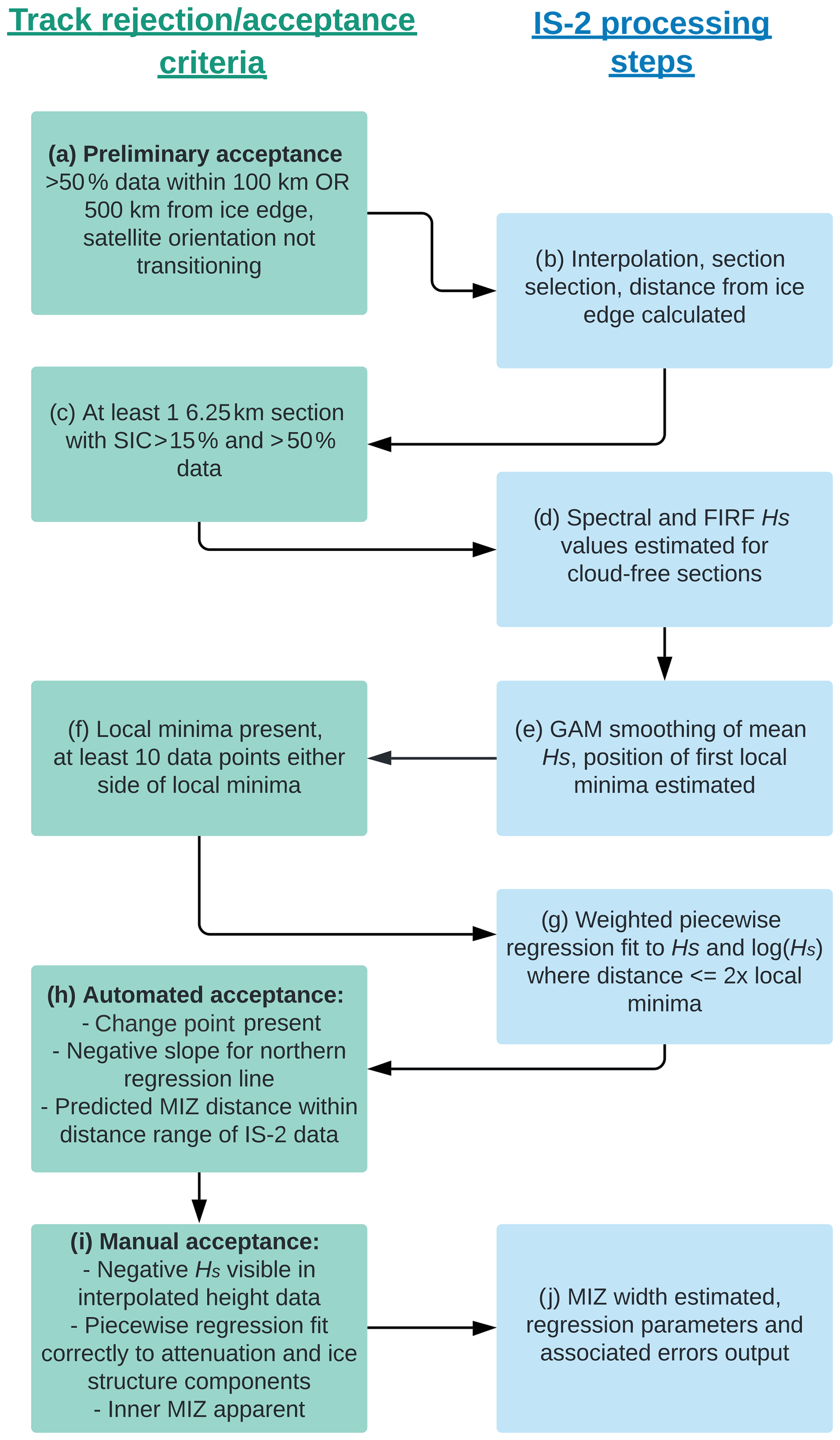
Accepted tracks were required to contain at least 10 valid 6.25 km sections for automated change-point segmentation (Fig. 1f). Following this step, any tracks with a positive gradient in the outer attenuation-dominated region were discarded. If the estimated wave penetration width was larger than the sea ice zone width (i.e. due to Hs attenuation extrapolation in regions of data gaps), the track was discarded (Fig. 1h). As a result, cases of a complete MIZ from the ice edge to the continent are likely to be erroneously discarded (a condition likely to occur in the narrow sea ice zone throughout much of East Antarctica or in the Bellingshausen Sea (Massom et al., 2008). Method improvements are required to account for these cases and will be discussed later.
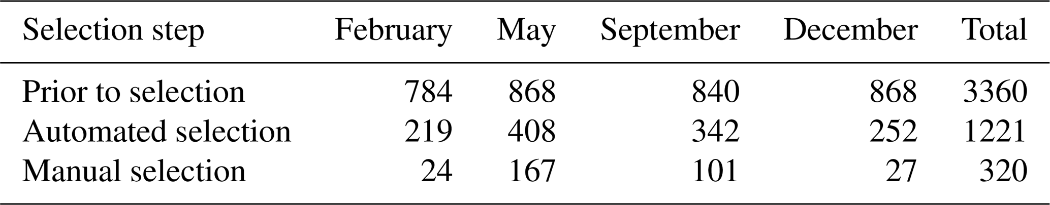
In order to ensure accurate wave penetration width estimation, manual selection was undertaken to remove cases where no wave attenuation was apparent (largely arising due to cloud cover over the region experiencing attenuation) or the attenuation models were clearly incorrectly fit (primarily due to Hs contributions from ice structure in the attenuation-dominated region; Fig. 1i). Wave attenuation was manually assessed by identifying the presence or absence of a triangular-shaped “envelope” of wave decay in the height data, showing as large positive and negative heights at the ice edge which attenuate with increasing distance into the sea ice (Horvat et al., 2020). The next criterion for this manual assessment was that the change point of the piecewise regression occurred at the transition from attenuation-dominated to ice-structure-dominated regions. To avoid high uncertainty in wave penetration width estimation due to missing (cloud-masked) data, tracks were further excluded if the boundary between the attenuation-dominated and ice-structure-dominated regions was obscured (by cloud). Due to the considerable manual overhead, four months of 2019 were analysed and presented here. Table 1 gives the number of tracks prior to track selection and after automated/manual selection in each month.
Table 1Number of tracks in each month (of 2019) remaining after automated filtering and manual filtering were applied. Tracks are split into ascending and descending components; i.e. there are two tracks per data file.
For the purposes of validation of IS-2-retrieved attenuation, Hs was directly measured from a deployment of five wave-sensing buoys and used to validate the Hs estimates derived from IS-2. Co-locations of IS-2 tracks and wave buoys were first identified, prioritising temporal proximity (within 6 h) over spatial proximity (within 400 km) under the assumption that wave conditions decorrelate quickly with time (a lag of 6 h reduces the autocorrelation coefficient to between 0.79 and 0.95 for the five buoys in this buoy deployment). Tracks containing a buoy co-location were then analysed to find the closest (spatial) measurement of Hs for comparison. IS-2-derived Hs measurements at these locations were also compared to a modified version of the Horvat et al. (2020) technique for estimating wave-affected fraction. The modification allows along-track (rather than gridded, as published) estimates of the wave-affected fraction using each IS-2 beam, along a 50 km sliding window.
Two case studies (Table 2) are presented to demonstrate the methods involved in directly detecting the presence of waves in the IS-2 height data and measuring their attenuation to find the inner MIZ boundary. Cases from September and February in 2019 are chosen to illustrate the performance of the wave penetration width estimation under different wave/ice conditions.
Table 2Summary of the two case study tracks. Latitude and longitude of the along-track ice edge location are provided.
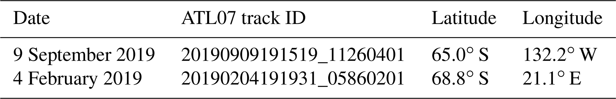
4.1 Case study from 9 September 2019
Figure 2a shows IS-2 heights observed from the ice edge to the continent. Negative heights indicative of wave passage (Horvat et al., 2020) were visible in all three strong beams (only centre beam shown) within ∼ 180 km of the ice edge. This region exhibits a distinctive attenuation envelope. Note that most height contributions due to tides, inverse barometer effects, geoid undulations and mean sea surface have been removed by the ATL07 algorithm (Kwok, 2019). Although some residual remains, these corrections are sufficient for the purposes of visual detection of wave attenuation during the manual filtering in this study. Increasing heights at around > 800 km from the ice edge indicate a transition to thicker ice. SDF-filtered altimetric heights displayed varying signal amplitude (outer 200 km shown in Fig. 2b–e). In this case, the largest heights were present in the data filtered with the SDF with a centre wavelength of 498 m. Waves of this wavelength appeared to penetrate up to ∼170 km from the ice edge.
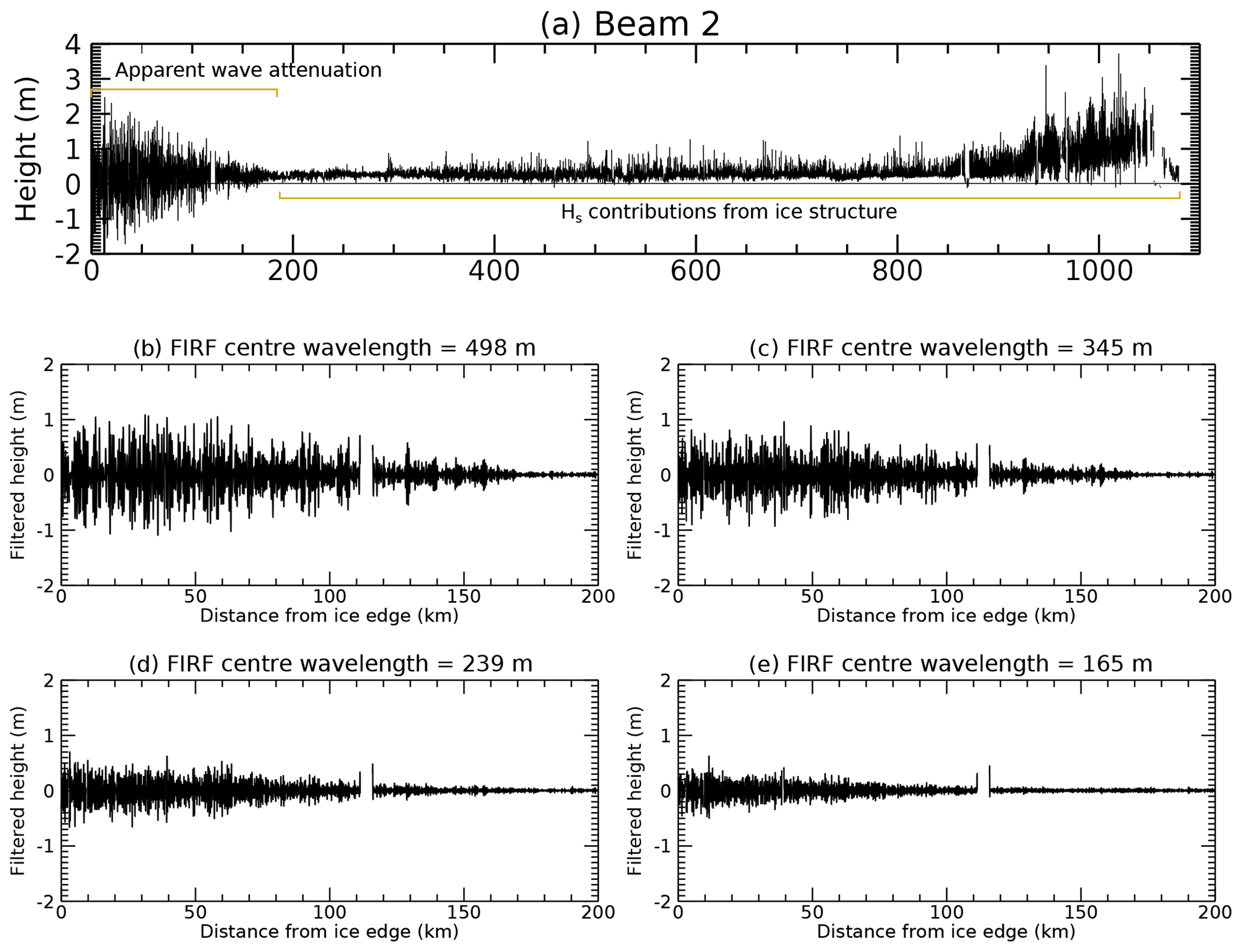
Figure 2(a) Resampled segment heights from the central strong beam, for case study 1. Data acquisition start time is 2019-09-09T19:15:19Z (timestamps follow standard Zulu time format throughout, where the date format is year-month-day). (b–e) SDF-filtered heights for each of the four FIRFs used in wave penetration width estimation, for the first 200 km of the track.
Further detailed analysis of the spectral amplitude as a function of distance from the ice edge, as well as GAM-based first local minimum estimation and change-point detection (for roughly delineating the attenuation-dominated boundary), and attenuation curve fitting (for estimating the limit of wave penetration) are presented in Appendix B.
To summarise the results of this case study, the presence of waves was apparent in the negative heights in the spatial data, and their attenuation was shown by the decrease in both positive and negative height values with increasing distances from the ice edge (the characteristic triangular envelope). This pattern of attenuation was visible until ∼ 180 km from the ice edge. Wave attenuation was also evident in the spectral domain, shown by the decreasing amplitude and narrowing of the spectral peak with increasing distance from the ice edge. SDF-based Hs estimates of wave penetration width ranged from 109 to 184 km (assuming linear attenuation and depending on the centre wavelength of the spatial domain filter). The three spectral Hs-based estimates were also within this range.
Underestimation of the MIZ width using the SIC-based technique for this case is shown in Fig. 3. In this figure Hm0 attenuation fit to distance from the ice edge (rather than using corrected distance) is given for visual comparison (for reference, the wave penetration width estimated using the corrected distance metric was 177 km). Agreement between the distance over which waves were visible and the wave penetration width distance derived from wave attenuation (i.e. panels a and c) provides high confidence in the methods of wave penetration width retrieval. A further case study, from 4 February 2019, is presented next, as evidence of this technique working well during the summertime sea ice minimum.
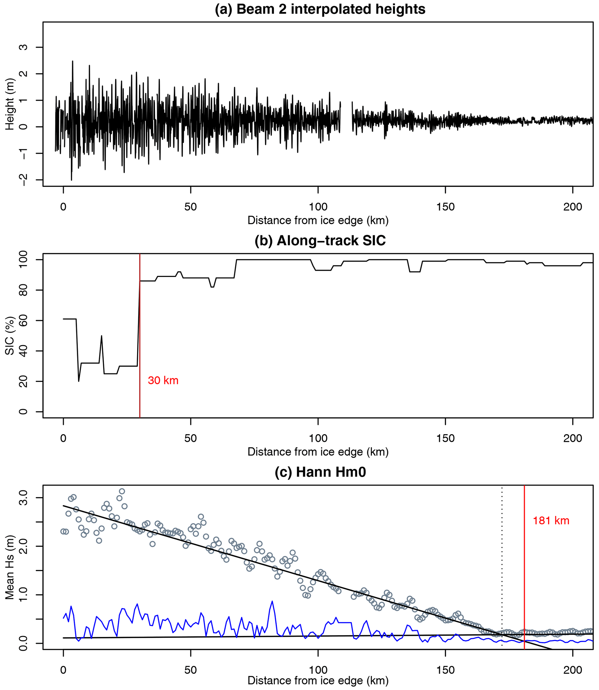
Figure 3Direct comparison of along-track (a) IS-2 beam 2 heights, (b) SIC-based MIZ width and (c) Hs and the resulting wave penetration width estimated by modelling wave attenuation, for case study 1. Data acquisition start time is 2019-09-09T19:15:19Z. The case illustrated here shows wave penetration width estimated using a linear fit to the Hann-windowed Hm0 values. Here, for comparison purposes, we perform the attenuation analysis (c) without consideration of SIC (i.e. on uncorrected distance).
4.2 Case study from 4 February 2019
The summer case study exhibited a narrower MIZ than the September case study presented above and smaller wave amplitude relative to inner-MIZ and pack ice structure variability (Fig. 4).
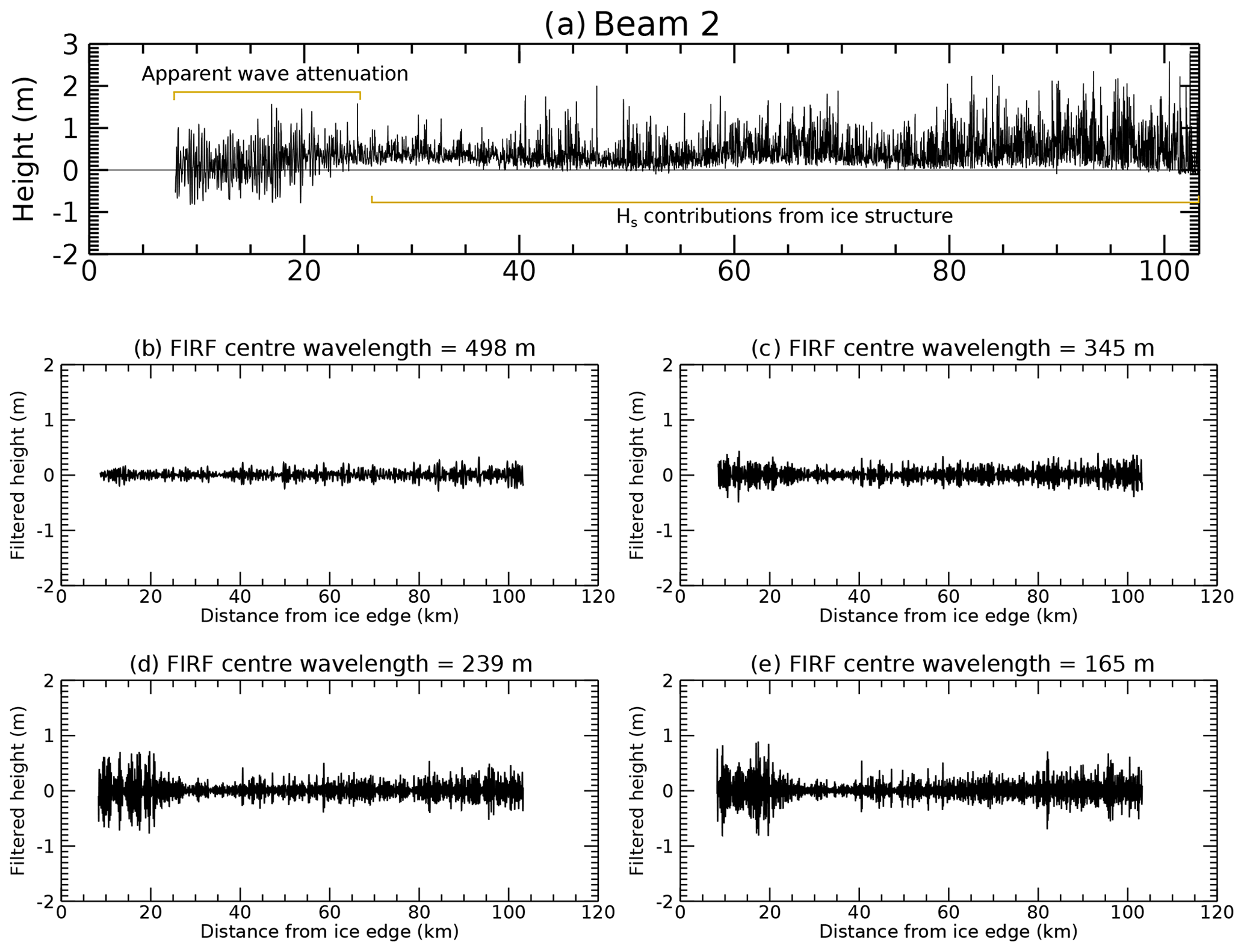
Figure 4(a) Resampled segment heights from the central strong beam, for case study 2. Data acquisition start time is 2019-02-04T19:19:31Z. (b–e) SDF-filtered heights for each of the four FIRFs used in wave penetration width estimation.
Further detailed analysis of this case study is presented in Appendix C. To summarise this case, negative heights were again observed near the ice edge, although the wave magnitude was lower in this case. Attenuation was visible until around 30 km from the ice edge. Similar patterns of attenuation to those in the first case study were also present here in both spatial and spectral domains, i.e. the presence of negative heights in spatial data and a downshift and narrowing of the spectral peak. Assuming linear attenuation, SDF-based Hs estimates of wave penetration width ranged from 31 to 58 km. The three spectral Hs-based estimates were also within this range. As with the previous case study, the SIC-based technique considerably underestimates MIZ width (with the 80 % SIC contour encountered at a distance of only 7 km from the ice edge, in contrast to the value of 33 km estimated using the Hann Hm0 technique with linear attenuation; Fig. 5).
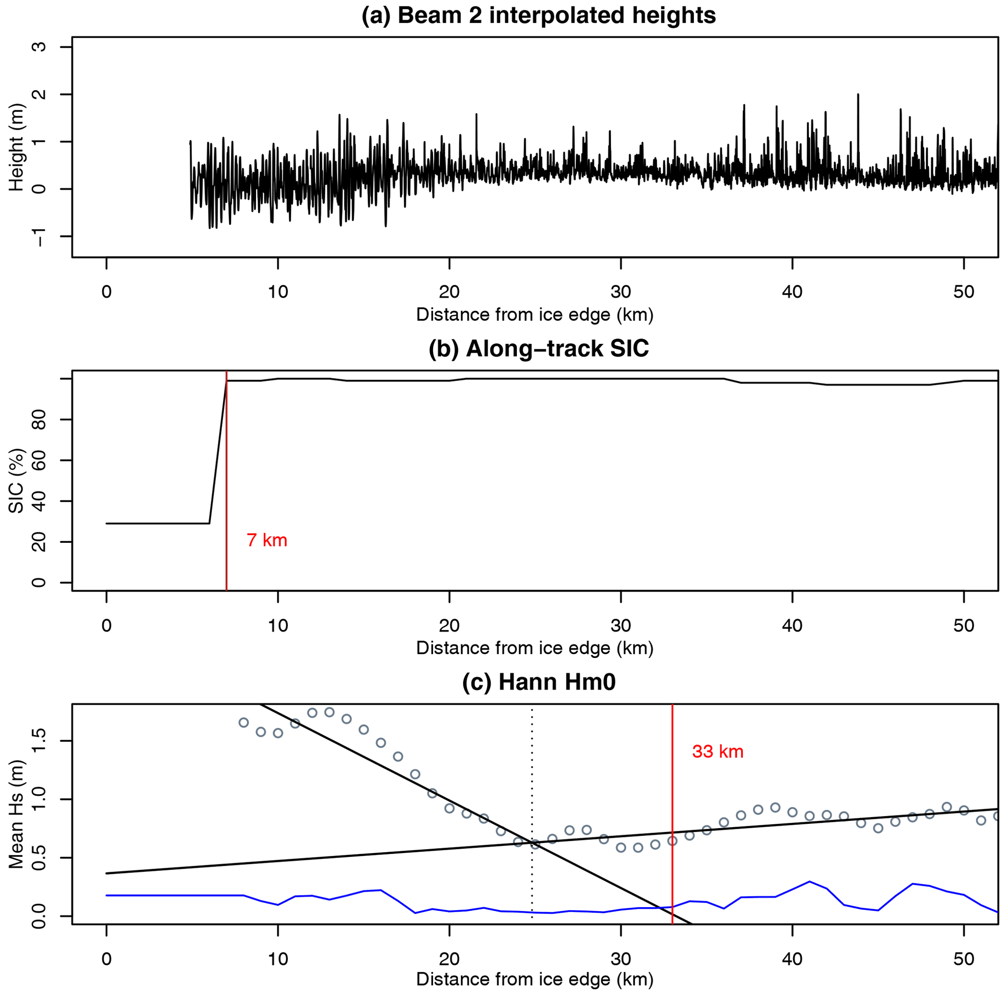
Figure 5Direct comparison of (a) IS-2 beam 2 heights, (b) SIC-based MIZ width and (c) wave penetration width, for case study 2. Data acquisition start time is 2019-02-04T19:19:31Z. The case illustrated here shows wave penetration width estimated using a linear fit to the Hann-windowed Hm0 values. Here, for comparison purposes, we perform the attenuation analysis (c) without consideration of SIC (i.e. on uncorrected distance).
4.3 Validation of IS-2 Hs against wave-buoy-derived Hs
From 80 tracks with a spatio-temporal separation (between buoy- and IS-2-measured Hs) of less than 400 km and 6 h, 10 were selected for comparison, based on the IS-2 track selection criteria presented above, with most rejected due to cloud cover. The mean time separation between buoy data acquisition and the corresponding IS-2 track overpass was 38 min. The mean distance from the buoy to the ice edge was 182 km (range 11 to 371 km). Validation of IS-2-derived Hs (in this case, the Hann-filtered Hm0 technique was used, but all gave similar results) against buoy measurements is presented in Fig. 6 and was found to be very sensitive to their spatial separation (i.e. waves decorrelated quickly with distance). For tracks within 200 km of the buoy measurement, Pearson's correlation coefficient r was 0.94 (but with only three tracks); however this remained high at r=0.72 when buoy–satellite conjunctions within 300 km were considered (six tracks). For these six conjunctions, the mean distance to the ice edge was 122 km; i.e. the buoys are generally closer to the ice edge than the satellites. Given the high orbital inclination of IS-2, with sub-satellite tracks aligned close to north–south at this latitude, this means most of the separation between the nearest pass of the sub-satellite track and the buoy occurs in the east–west direction (cloud coverage notwithstanding). It is assumed that the spatial decorrelation of wave height in sea ice is highly anisotropic (i.e. the wave height field varies quickly from north to south as waves become attenuated in that direction but slowly from east to west, assuming incident waves from the north and a perpendicular ice edge); however a more in-depth study of the spatio-temporal decorrelation of wave height is required to fully understand how wave buoys can be best used to validate IS-2-derived heights.
The correlation is significant for spatial separation of less than 300 km. For conjunctions within 300 km, the Hs regression slope was 0.44, i.e. less than 1.0, indicating that IS-2 underestimates Hs (by a factor of ∼ 2.25 in this case). This is not surprising given the fundamental difference in measurement technique; however the high correlation and positive slope, particularly at < 300 km separation, give confidence in the approaches demonstrated here. For the same 10 IS-2 tracks, the correlation between the wave-affected fraction (from the along-track-modified Horvat et al., 2020, technique) and IS-2-based Hs retrieved here was r=0.55 (049), indicating a significant correlation despite differences in wave estimation technique. More detailed comparison of these two IS-2-based wave estimation techniques is planned for the future.

Figure 6Validation of IS-2-derived Hs against wave buoy data, using Pearson's correlation coefficient (black line) and regression slope (red line), as a function of the closest distance between track and buoy. The regression slope of less than unity indicates that IS-2 underestimates Hs. The blue line indicates the correlation coefficient between the Hs technique presented here and the wave-affected fraction using a modified along-track wave-affected fraction metric (after Horvat et al., 2020). The dashed line indicates the significance threshold for the blue and black lines.
Based on the case studies presented in Sect. 4.1 and 4.2 and other tracks assessed during manual filtering, the SDF technique was chosen to estimate wave penetration width. The median value of the MIZ distance determined in four SDF wavelengths (165, 239, 345 and 498 m) was used as the wave penetration width metric to reduce the reliance on attenuation in one particular wavelength range. The advantages of the SDF technique over the spectral methods were two-fold: taking the median of wave penetration width estimates from SDFs in the wavelength range of 165 to 500 m enabled increased sensitivity to waves within a wavelength range that was assumed likely to physically impact the ice and was prevalent in the Antarctic MIZ (see Fig. 2 in Stopa et al., 2018a) and minimised Hs contributions from ice structure. The simplicity of applying SDFs and relevant amplitude correction in addition to the absence of the effect of spectral noise caused by convolution of data gaps was a further advantage (Murphy et al., 2007). A comparison between techniques is presented in Appendix D, indicating that all techniques considered here are highly correlated.
4.4 Attenuation model comparison and wave penetration width uncertainty quantification
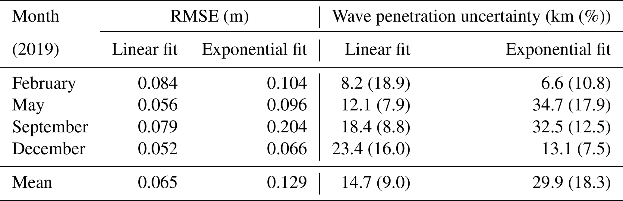
The RMSE residual between observed Hs and the fit in the attenuation-dominated region was approximately 2 times smaller for the linear attenuation model than the exponential fits over the four months in the study period (Table 3), indicating that the linear attenuation model provided a better fit for the cases studied here. Wave penetration width uncertainty, calculated from uncertainty in the y intercept and slope of the fit (see Table 3), was larger for the exponential attenuation model in May and September and ranged from ∼ 8 % (linear, May and September) to ∼ 19 % of the overall wave penetration width (linear, February).
Table 3Uncertainty statistics of SDF median wave penetration width estimates by month. Wave penetration uncertainty is the error in wave penetration width calculated from the slope and intercept uncertainty (which were quadrature-added to the window size, 6.25 km), shown as absolute values (km) and as a percentage of the mean wave penetration width.
4.5 SDF-based wave penetration width estimation compared to the SIC-based MIZ width technique
The traditional SIC-based MIZ width estimation gave lower estimates than those derived from SDF Hs attenuation in all months analysed. A comparison of these techniques is shown in Fig. 7 (exponential results have been omitted here due to the larger attenuation model fit residuals and uncertainties described above but are similar). SIC-derived MIZ width and SDF-derived wave penetration estimates were closest in February, when linear SDF-derived estimates were ∼ 2.3 times larger than SIC-derived estimates. SDF-derived estimates were ∼ 4.6 and 6.7 times wider in May and September, respectively. The largest differences between estimates occurred in December, with a regression slope of 14.9.
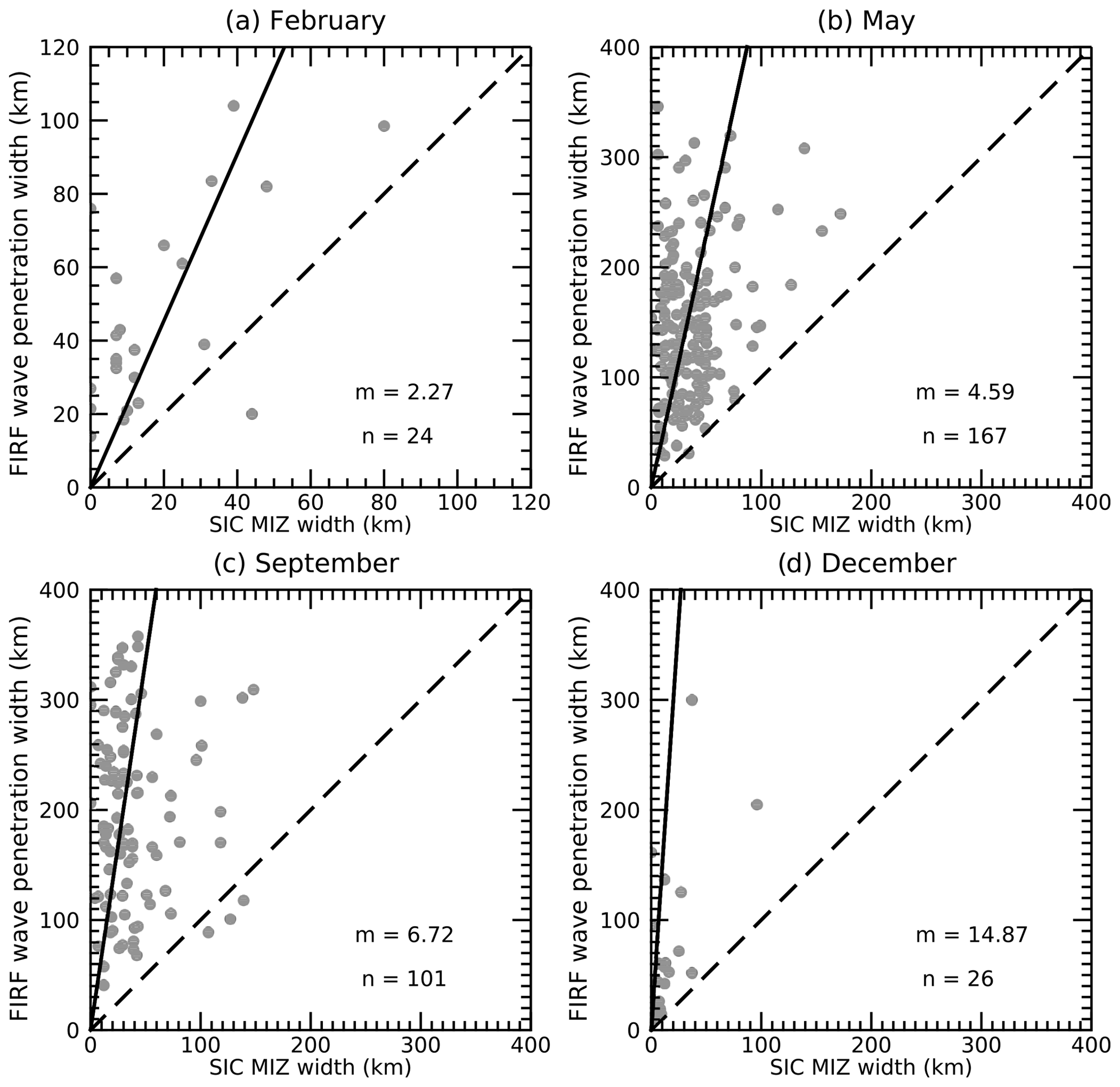
Figure 7Comparison between SIC-derived MIZ width and SDF-derived wave penetration width estimates for each month. SDF wave penetration width estimates were derived using a linear fit to the attenuation curve of Hs estimates. The slope (m) and number of samples (n) for each month are presented. The solid black line shows the linear best fit forced through the origin, and the dashed line represents the 1:1 reference. All panels range from 0 to 400 km except panel (a) (0 to 120 km).
4.6 MIZ and wave penetration width seasonality
For the same set of tracks (i.e. those which passed the automated and manual track selection mentioned above), median SIC-derived MIZ width estimates were far narrower than SDF-derived wave penetration widths in all months (Fig. 8). SDF-derived wave penetration widths were deepest in September and narrowest in February. Using the SDF technique, wave penetration widths in excess of 600 km are observed to occur in May, September and December, whereas SIC-based estimates of MIZ width never exceed 200 km. We note that SIC-derived MIZ width is wider in May than September, in contrast to the IS-2-derived result presented here. The Southern Ocean Hs is higher in September than in May (Young et al., 2020), possibly indicating that the IS-2-derived wave penetration presented here is a more realistic representation of the MIZ than the SIC-derived metric; however wave–ice interaction model studies are required to confirm this.
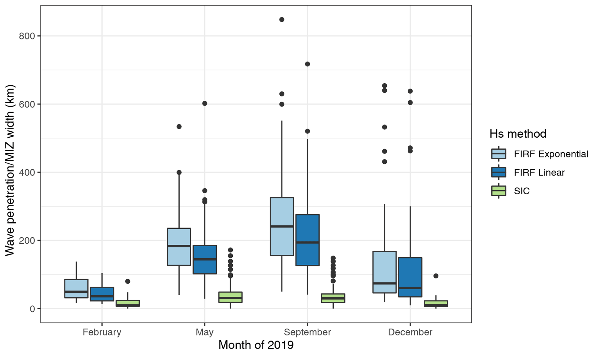
Figure 8IS-2-derived wave penetration width estimates by month for the SDF methods (assuming linear and exponential attenuation) compared to the SIC-derived MIZ widths. The median and first and third quartiles are indicated by boxplot centre line and hinges. Whiskers extend to 1.5 times the interquartile range, and data beyond this are shown as individual points.
5.1 Towards improved definition of the MIZ
MIZ width estimates from SIC were far narrower than wave penetration width values from IS-2, and the disparity between SIC and wave presence in sea ice was illustrated in the case studies demonstrated in Sect. 4.1 and 4.2. It was then shown that this result occurs in all four months studied. This work is further evidence that the SIC-based MIZ may not accurately reflect the presence of waves. Both Vichi et al. (2019) and Alberello et al. (2021) detected waves in unconsolidated yet high-concentration (100 %) sea ice, through which waves could easily propagate. Knowledge of SIC distribution alone (without ice type or thickness information) is inadequate for understanding the evolution of the MIZ, especially during an extreme polar cyclone (Vichi et al., 2019) or compaction events (Massom et al., 2008), when the presence of strong on-ice winds may lead to wave penetration within extremely compressed (100 %) SIC. This new technique presents a potential alternative to the SIC-based definition of the MIZ and may allow the study of MIZ response to extreme wave events in more detail.
In contrast to the findings presented here, Horvat et al. (2020) found IS-2-derived “wave-affected” regions had a smaller spatial extent than the SIC MIZ across all seasons and hemispheres. We suggest two potential reasons for this discrepancy. First, the Horvat et al. (2020) method cannot record waves with smaller amplitudes than sea ice freeboard variability and likely underestimates the areas where waves are truly present. Second, Horvat et al. (2020) developed a gridded product from all IS-2 tracks, whereas we focused on a subset of IS-2 tracks in which waves were manually identified. Thus while there is high correlation between both estimates, the inclusion of many tracks without active waves in a gridded product reduces the overall extent of the wave-affected MIZ.
The inner wave penetration boundary was here defined as the point where Hs equalled the estimated error in the surface heights. The estimates of wave penetration width presented here (especially when assuming exponential decay) likely include small-amplitude waves in the inner MIZ that may have energies too small to “significantly impact the dynamics of sea ice”, as considered a physical component of the MIZ in Weeks (2010). It is then necessary to consider what magnitude of wave energy (or Hs) has sufficient impact on sea ice properties, e.g. the threshold when waves are energetic enough to break sea ice (Dumont et al., 2011; Williams et al., 2013a, b; Bennetts et al., 2015; Williams et al., 2017). This is less straightforward as it requires knowledge of the geometric and mechanical properties of the ice cover (including thickness, floe size, elastic modulus) to quantify when stresses in the ice exceed the break-up strength. Sutherland and Dumont (2018) defined the MIZ as the distance from the ice edge over which modelled compressive forcing from wave stress was greater than or equal to that from wind stress. Through the techniques presented here, this “dynamics-impacted” MIZ could be studied using an adjusted (higher) Hs threshold.
5.2 Hs estimation method and caveats associated with this work
The high correlation among IS-2 wave penetration width estimation methods indicated that these results were relatively insensitive to Hs calculation method. The selection of a wavelength subset for the SDF median estimation of Hs did not significantly influence wave penetration width estimates, as similar results were shown for the Hm0 estimates (i.e. integrated over 16 to 1500 m, wave periods from 3 to 30 s) and the standard-deviation-derived Hs (where no bandpass filtering was applied). This indicated suitability for the choice of SDF-based selection, with the potential benefit of increased sensitivity to surface gravity wave wavelengths most commonly present in the Antarctic MIZ and most likely to impact sea ice.
There are a number of caveats associated with the wave penetration width estimation techniques presented here. Although most manual rejection of IS-2 tracks was because of cloud obscuration of the MIZ, there may be other cases excluded because no attenuation visibly occurs, such as due to quiescent wave conditions north of the ice edge. In such cases, SIC-derived MIZ estimates may be wider than those based on attenuation. This selection bias favours obvious attenuation occurring when open-ocean Hs is large. In these (unrepresented) offshore low-Hs cases, an SIC-based measurement of MIZ width is also inappropriate.
A bias may also be introduced by exclusion of tracks where wave attenuation occurs from the ice edge to the Antarctic continent. Such cases are likely to occur around the time of the sea ice minimum, particularly in East Antarctica and the Bellingshausen Sea, where sea ice extent is lower than in the Weddell or Ross seas. In addition, it is possible that times of northerly winds may bring both high apparent Hs at the ice edge (favouring visible and obvious attenuation) and a compacted ice edge, resulting in a narrower SIC-derived MIZ width estimate. Consideration (and elimination) of such potential biases should form the focus of subsequent work.
5.3 Wave attenuation model
Exponential decay, with the decay rate as a function of wave frequency, is widely accepted as an appropriate form for modelling wave attenuation (Meylan et al., 2018), is predicted by linear theory (Squire, 2020), has been demonstrated by observational wave buoy studies (Kohout et al., 2020) and has been implemented in mathematical models (Meylan et al., 2018). However, the mean RMSE and wave penetration uncertainty statistics presented here were smaller for the linear than exponential fit. This may suggest non-linearity in energy transfer during attenuation, perhaps caused by variation in ice thickness, which has been shown to strongly affect attenuation rates (De Santi et al., 2018), or energy input from wind to waves in unconsolidated sea ice, which is not currently accounted for in contemporary wave models (Rogers et al., 2020). The aforementioned potential bias towards times of larger wave heights may also play a role in the apparent better fit of linear attenuation (Kohout et al., 2014; Montiel et al., 2018) due to the occurrence of non-linear dissipation mechanisms including wave overwash of floes and breaking (of steep waves) close to the ice edge (Squire, 2018). Seasonal effects on attenuation may also be expected due to seasonal variability in ice cover and type (e.g. Doble et al., 2015). The prevalence of thinner, unconsolidated pancake ice during the Antarctic growth season may result in lower attenuation rates. Meylan et al. (2014) found no change in Hs within the outer 80 km of the Antarctic MIZ in September, where there were small floes (10 to 25 m diameter) present and low SIC. Non-linear viscous dissipation may be a dominant mode of wave attenuation in unconsolidated ice types (Squire, 2020). Correction for incident wave direction (Kohout et al., 2020) and noise effects (especially at lower frequencies; Thomson et al., 2021) should also be considered in future work to ensure accuracy in attenuation coefficient retrieval.
5.4 MIZ seasonality
Wave penetration width seasonality agreed broadly with that expected from seasonal trends in Southern Ocean Hs, with larger incident waves in winter months able to penetrate further into the MIZ, matching the seasonality of Young et al. (2020). We draw attention to a large discrepancy between SIC-derived MIZ widths and IS-2-derived wave penetration widths: SIC MIZ width was 4.6 and 6.7 times lower than linear SDF-derived wave penetration width in May and September, respectively. SIC-based studies of MIZ seasonality have shown a peak in MIZ area in October/November, after the annual sea ice area maximum (Uotila et al., 2019), whereas the wave-affected fraction metric described by Horvat et al. (2020) was unexpectedly low in November 2018. Although only four months were assessed in the present study, improved automation of these techniques and their application over the whole IS-2 data record (September 2018 to present) may improve our understanding of seasonal MIZ dynamics and should be prioritised for future work.
Seasonality and sea ice characteristics also play a role in the reliability of wave penetration estimates. Thicker multi-year or first-year ice near the ice edge in summer increases the difficulty of differentiation between wave presence and ice structure, necessitating manual removal of such cases. By way of comparison, March to September is characterised by pancake ice present at the ice edge, providing a more homogeneous environment in which to observe attenuation. In the period of rapid spring ice retreat (November to early February), further challenges to accurate wave penetration estimation occur due to the complex ice edge morphology and the development of open-water regions near the continent. Complexity in the spatial distribution of retreating ice edge can result in the orientation of IS-2 tracks not being orthogonal to the ice edge and the measurement of waves along the boundary of sea ice rather than into the pack, giving spurious estimates for attenuation. The variable distribution of open water at this time may increase the incidence of observing multiple wave directions due to local wave generation, potentially impacting the reliability of attenuation estimates. The highest disagreement between IS-2 and SIC was observed in December, and this is likely linked to such complexities during rapid retreat. The lowest disagreement between IS-2 and SIC was observed in February, likely because of the smaller total sea ice extent at this time (Eayrs et al., 2019).
5.5 Further improvements
In addition to those previously suggested, one large improvement to this work would be the consideration of incident wave direction in spectral estimates. A north–south wave propagation direction has been assumed in most previous studies on wave attenuation (e.g. Kohout et al., 2014) and is similar to the along-track wave direction assumed here. If the incident wave direction were offset from the IS-2 track, the wavelength would be underestimated by a factor of cos (θ), where θ is the angle between the incident wave direction and the satellite track. This potentially results in invalid assumptions for the SDF wavelength choice, leading to a misrepresentation of these parameters. Wave direction corrections, for example following the methods in Kohout et al. (2020), would allow physically meaningful retrievals of wavenumber and spectral width characteristics. Wave direction will also affect the corrected distance calculation using SIC values retrieved, enabling them to be representative of SIC that waves travelled through. As there remain uncertainties in wave reanalysis products (especially within sea ice), the remotely sensed wave direction from the forthcoming SWOT satellite radar altimeter (Armitage and Kwok, 2021) may provide improved wave direction estimates.
In addition to Hs, spectral width may be another important parameter to consider for wave penetration width estimation. Both case studies presented here exhibited a prominent spectral peak associated with the presence of waves, although the magnitude of the peak wavelength varied due to the characteristics of the incident wave field. In contrast, areas of ice structure displayed a very different signature of Brownian noise. The difference in spectral shape between these two regimes may be a more robust way of distinguishing the presence of the MIZ (for example from isolated sections), rather than requiring a full track of attenuation. If this method were applied, an estimate of the Brownian noise threshold associated with ice structure (following the methods in Thomson et al., 2021) may provide a suitable cut-off for frequencies and power spectral amplitude over which to estimate spectral width. Consideration should also be given to the use of the lower-level ATL03 dataset from IS-2, which reports individual geo-located photon reflection locations, and other techniques which do not require resampling of along-track data (e.g. non-uniform Fourier transforms), as these may preserve important spectral information lost in the production of the ATL07 segments.
The application of spectral and spatial techniques to ICESat-2 data presented here gives an effective means of remotely determining wave attenuation in sea ice. Improved understanding of wave attenuation in ice, facilitated by a larger number of widely distributed records of attenuation from IS-2, may be applicable for incorporation into wave and sea ice models. Here, many tracks were too cloud-affected to give a complete record of wave attenuation. However, this technique may assist in developing such a record by validating other large-scale MIZ width estimates achieved from microwave-based remote sensing techniques, including scatterometers and the forthcoming generation of synthetic aperture radar altimeters (Lubin and Massom, 2006). This attempt to remotely characterise MIZ wave penetration width is a step towards improving our understanding of the interactions in this zone, with widespread application for studies concerning MIZ ecology and physical processes.
The spectral analysis of IS-2 data applied here seeks to obtain power spectra whose amplitudes are directly related to those of the underlying waves. This is made difficult by the (sporadic) absence of data due to cloud and the application of windowing functions. Both of these effects lead to a decrease in the sum contributing to the mean-square amplitude of the altimetric height segment. In accordance with Parseval's identity, the average spectral power also decreases according to
where ck denotes the mean-removed heights (potentially attenuated or set to zero) along a segment of the track containing N points and Cn denotes the components of its digital Fourier transform (DFT). (Note that the position of the factor depends on the form of the DFT being used.)
Following Press et al. (1992, their Sect. 13.4), compensation for the effect of windowing can be achieved by replacing the factor used to calculate spectral amplitudes from with , where
and wj is the window function weighting applied to each ck before the application of the DFT.
The usual application of a windowing correction sees window amplitudes wj summed over all N points. In the presence of missing data, the windowing function can be reinterpreted to be the product of the windowing function and a missing data mask, equal to unity only where valid data are present. To adapt the Wss correction, an interpretation where wj is zero within data gaps is applied, such that
where G is the set of indices of good data. This acts to scale the spectral coefficients back up to the (physical) wave amplitudes and to do it in a way that includes the impact of the distribution of the missing data on the windowing function.
Here we present further detailed analysis of the 9 September 2019 case study.

Figure B1Mean power spectral density as a function of wavenumber and distance from the ice edge, for case study 1. Data acquisition start time is 2019-09-09T19:15:19Z.
Figure B1 presents the power spectrum for the entire track. Narrowing of the spectrum from 0 to 200 km is evident. From ∼ 250 to 800 km there is a region of low spectral amplitude due to low variability in height. After 800 km, high spectral amplitude is spread across a wider wavenumber (2 wavelength) range. This distribution of spectral amplitude is very different to that of the first 200 km.

Figure B2Hann-windowed power spectra of sections close to the ice edge (a) and in the inner pack (b), for case study 1. Data acquisition start time is 2019-09-09T19:15:19Z. The colour scale indicates distance from the ice edge. Power spectral estimates were smoothed with a 5-point moving average. The black line in the upper right of panel (b) represents the spectrum of a Brownian noise signal (−20 dB per decade).
Power spectra of individual 6.25 km sections within 200 km of the ice edge (Fig. B2 – Hann-filtered spectra shown only; boxcar-filtered spectra were similar) displayed a prominent peak wavenumber of ∼ 0.0015 m−1, corresponding to a wavelength of 650 m (wave period of ∼ 20 s). This is similar to the dominant wavelength suggested by the FIRF analysis. Power spectra of sections close to the Antarctic continent (> 817 km from the ice edge; given in Fig. B2b) peaked at very short wavenumbers, corresponding to very long wavelengths. In this region, the spectral shape displayed a near-monotonic decrease in spectral amplitude, characteristic of Brownian noise (Gilman et al., 1963). For this section of ice > 817 km from the ice edge, total spectral amplitude increased with increasing distance from the ice edge as the variance in surface height increased.
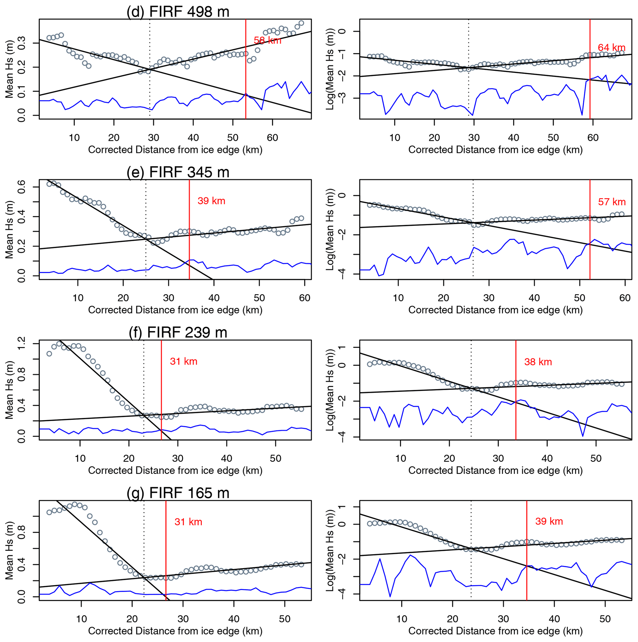
The steps involved in attenuation model fitting and wave penetration width estimation are demonstrated in Figs. B3, B4 and B5 for all methods of wave penetration width estimation presented here. The GAM smoothing technique is able to effectively estimate the first local minimum (dashed red lines, Fig. B3). The subsequent change-point estimation using segmented linear regression identified the transition from wave-attenuation-dominated Hs to ice-structure-dominated Hs (dotted black lines in Figs. B4 and B5). Final wave penetration widths (red lines in Figs. B4 and B5) were estimated from the intercept between modelled attenuation (outer section of the segmented linear regression) and the estimated error in Hs estimates. Hs was expected to approach zero when waves were fully attenuated (i.e. no surface variations in the absence of waves). However for all Hs estimation methods there was a positive offset in Hs after the transition to the ice-structure-dominated region, likely associated with Hs contributions from variations in ice thickness. This offset was slightly lower for the SDF Hs estimates than the other methods which measured the amplitude of the whole spectrum (Figs. B4 and B5). The model fit to the attenuation appears reasonable (Figs. B4 and B5), and the linear attenuation model appears to fit the data better than the exponential model in this case. Assuming linear attenuation, wave penetration width estimates range from 109 to 184 km, as estimated by the 126 and 498 m SDFs, respectively (with Hs-derived estimates falling within this range). Exponentially modelled wave penetration width estimates range from 179 to 263 km.
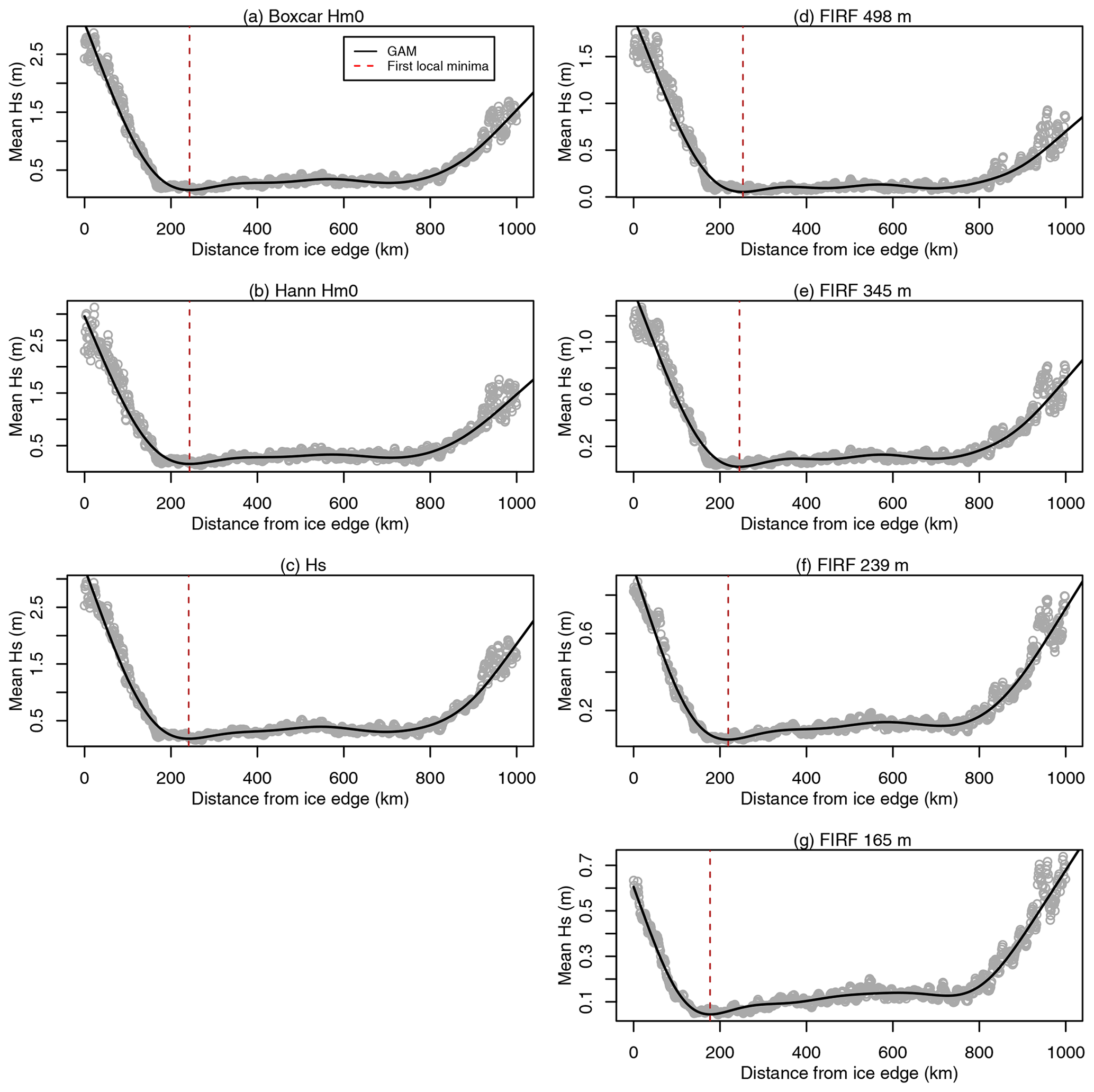
Figure B3GAM-based local minimum estimation for the spectral (left column) and SDF-derived (right column) estimates of Hs, for case study 1. Data acquisition start time is 2019-09-09T19:15:19Z. The section from the ice edge to 2 times the GAM-based minimum distance is used for change-point estimation.

Figure B4Wave penetration width estimation for the spectral Hs estimation methods, for case study 1. Data acquisition start time is 2019-09-09T19:15:19Z. The linear fit is shown on the left and exponential (by log-transforming the y axis) on the right. The grey scatter points show Hs estimates derived from each spectral analysis technique. The dotted black line represents change-point estimation of the piecewise linear regression. The blue line represents the quadrature-added uncertainty in Hs estimates. The estimated wave penetration width is marked by the vertical red line and labelled in terms of the equivalent uncorrected (actual) wave penetration width.
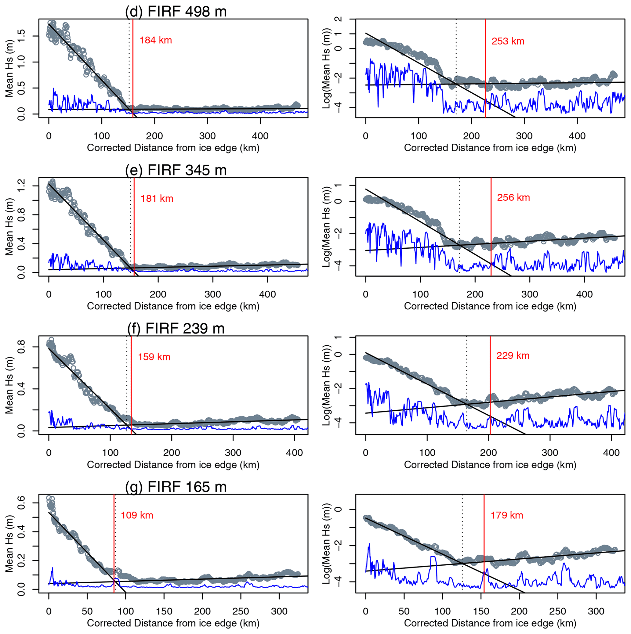
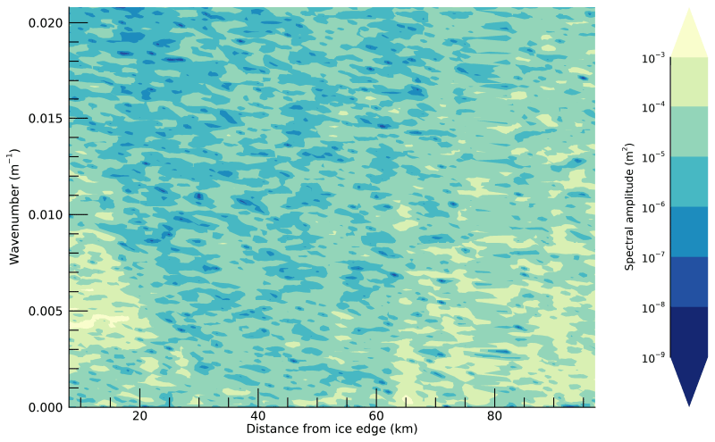
Figure C1Mean power spectral density as a function of wavenumber and distance from the ice edge, for case study 2. Data acquisition start time is 2019-02-04T19:19:31Z.
Here we present further detailed analysis of the 4 February 2019 case study.
The peak wavelength indicated by both the SDFs and Hann power spectra was ∼ 250 m (corresponding to a wavenumber of ∼ 0.004 and a period of ∼ 11 s; Figs. C1 and C2), shorter than that of case study 1 by ∼ 400 m.
Change-point estimation also performed well for this case study, despite fewer points being available for fitting compared to the other case study presented (Figs. C3, C4 and C5). Similarly to the September case study, Hs values did not reach zero at the end of wave attenuation (indicating ice structure contribution to apparent Hs at the transition point), and the “offset” here was again smaller for the SDF-based techniques (∼ 0.2 m for SDF-based Hs vs. ∼ 0.6 m for boxcar Hm0, Hann Hm0 and standard-deviation-derived Hs). Most methods resulted in an IS-2-estimated wave penetration width of 30 to 40 km, with the exponential attenuation model resulting in wider estimates.

Figure C2Hann-windowed power spectra of sections close to the ice edge (a) and in the inner pack (b), for case study 2. Data acquisition start time is 2019-02-04T19:19:31Z. The colour scale indicates distance from the ice edge. Power spectral estimates were smoothed with a 5-point moving average. PSD denotes power spectral density.
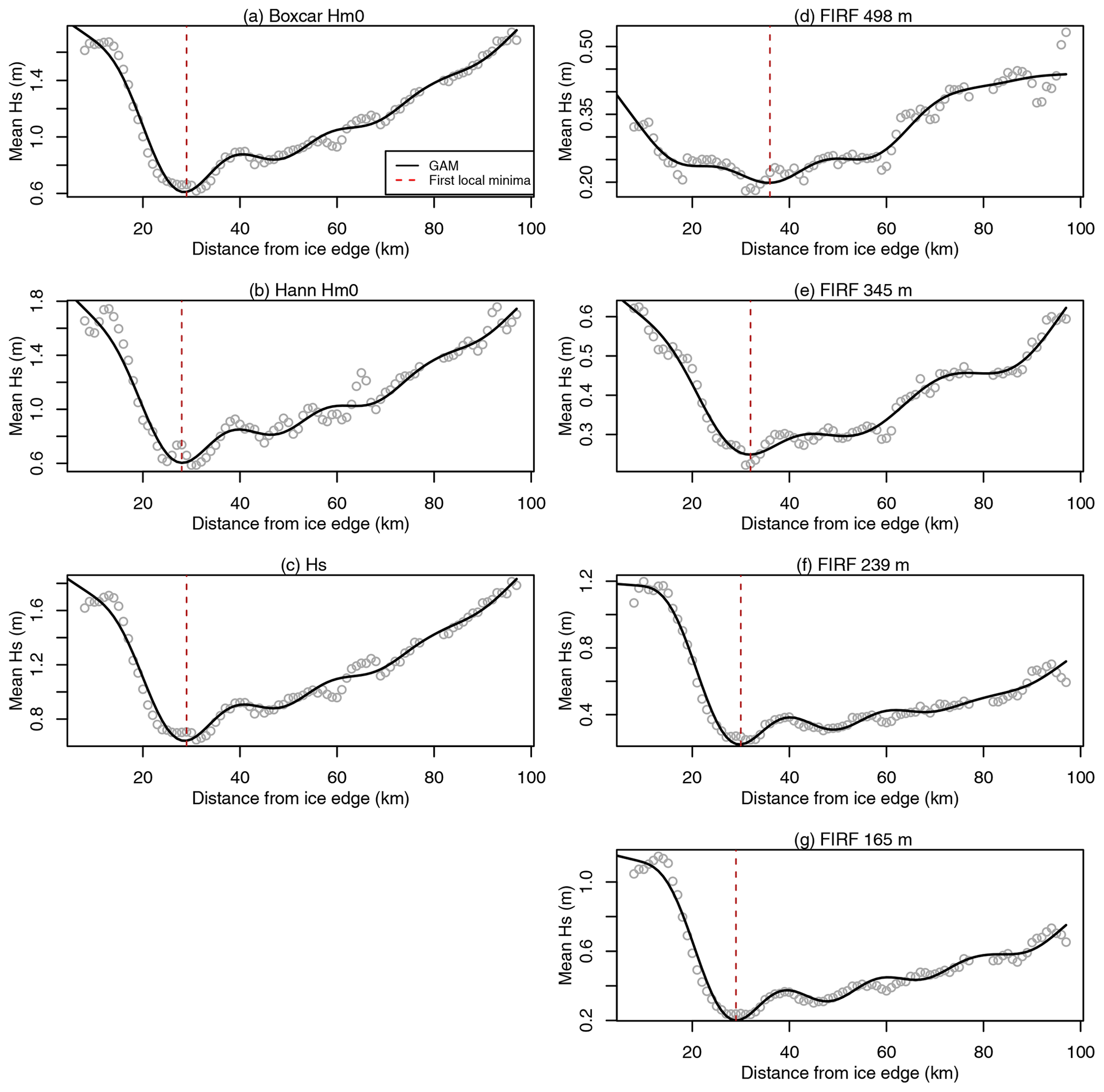
Figure C3GAM-based local minimum estimation for the spectral (left column) and SDF-derived (right column) estimates of Hs, for case study 2. Data acquisition start time is 2019-02-04T19:19:31Z. The section from the ice edge to 2 times the GAM-based minimum distance is used for change-point estimation.
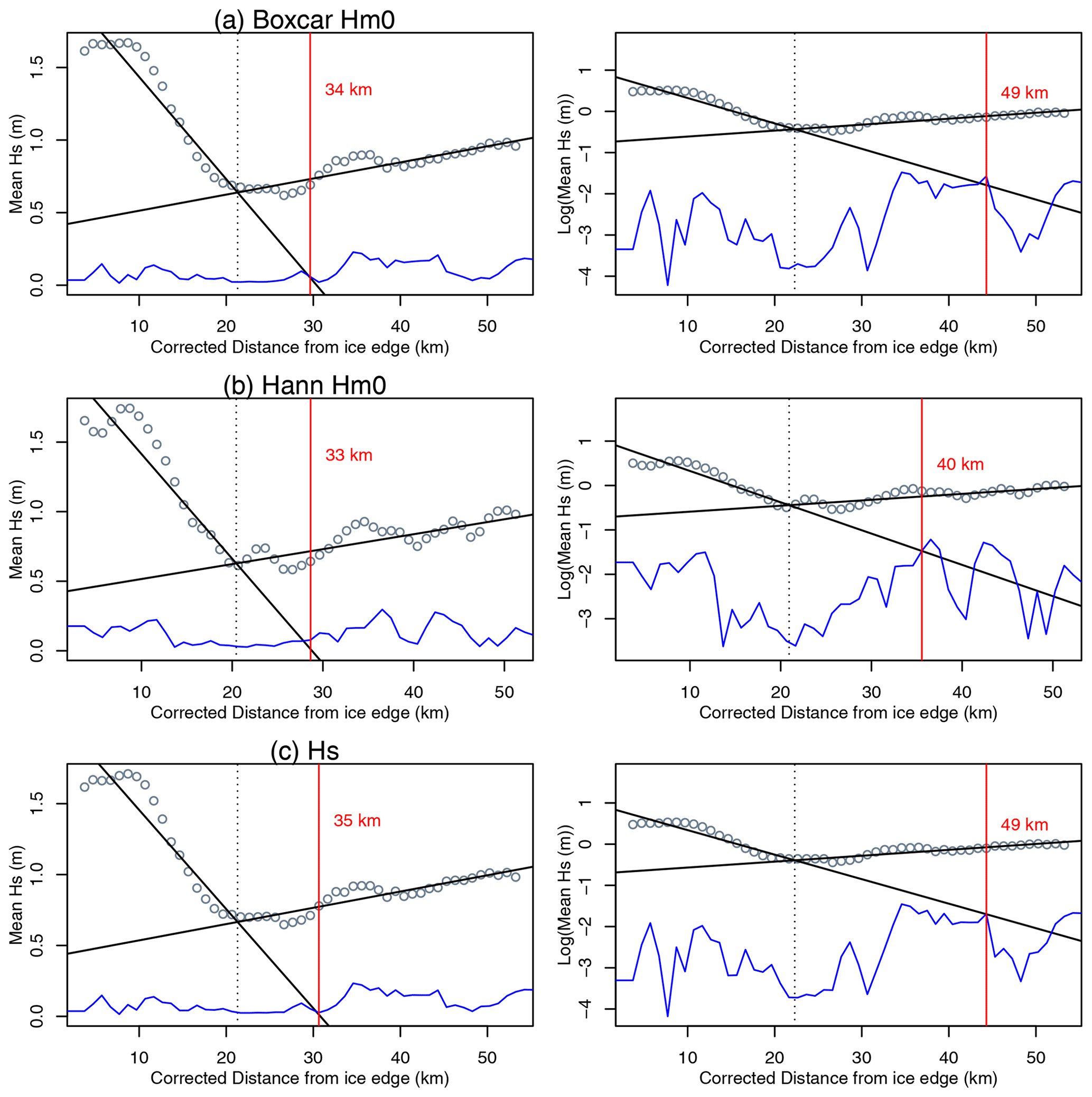
Figure C4Wave penetration width estimation for the spectral Hs estimation methods, for case study 2. Data acquisition start time is 2019-02-04T19:19:31Z. The linear fit is shown on the left and exponential (by log-transforming the y axis) on the right. The dotted black line represents change-point estimation of the piecewise linear regression. The blue line represents the quadrature-added error in Hs estimates. The estimated wave penetration width is marked by the vertical red line and labelled in terms of the equivalent uncorrected wave penetration distance.
There was a very high correlation between SDF median-derived wave penetration width estimates and those derived from all other Hs estimation methods (Fig. D1). The regression slope across all comparisons was in the range of 0.918 to 1.01, indicating robust agreement between all wave penetration width retrieval techniques. Pearson's correlation coefficient between the SDF-derived technique and all other techniques was between r=0.949 and r=0.978.
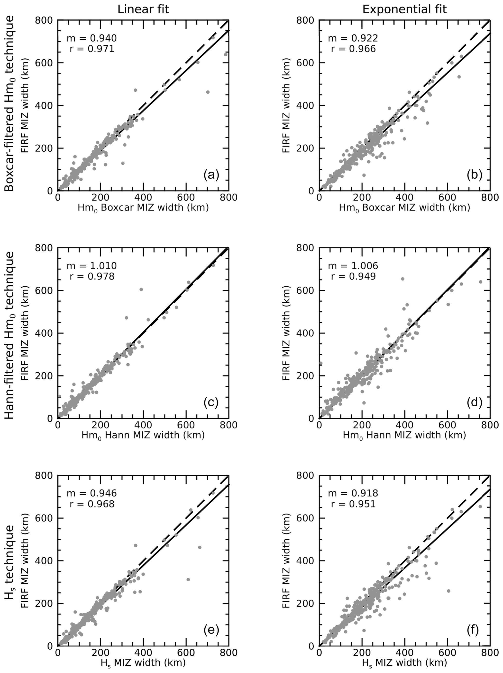
Figure D1Linear regression between SDF-based wave penetration width estimates and those based on Hm0 with boxcar (a, b) and Hann (c, d) windowing and the Hs estimate derived from the standard deviation of heights (e, f). Spectral analysis methods were compared for both linear (a, c, e) and exponential (b, d, f) attenuation modelling methods. Solid black lines show the linear regression (constrained to pass through the origin), with slope (m) and Pearson's correlation coefficient (r) values indicated in the top left of each plot. Dashed lines represent a slope of unity.
AMSR2-derived sea ice concentration data (using the ARTIST Sea Ice algorithm) were obtained from the University of Bremen. ICESat-2 sea ice height data (ATL07 product) were obtained from the National Snow and Ice Data Center (NSIDC). The wave–ice buoy data are available from the New Zealand Ocean Data Network (https://doi.org/10.17632/22hpw2xn3x.1, Kohout et al., 2021). Processed ICESat-2 data will be made available as an Australian Antarctic Data Centre archive in compliance with FAIR (findability, accessibility, interoperability and resuability) data standards upon paper acceptance. Code to reproduce these results are available at GitHub (https://github.com/Jill-Brouwer/Brouwer-etal-2022-MIZ-code; Brouwer, 2022).
All authors edited the manuscript. JB and ADF led the analysis, produced all figures, drafted the paper and coordinated co-authors. DJM advised on spectral and spatial analyses. PW, GDW and AK deployed the buoys and contributed to the analysis. AA and RAM assisted with wave–ice interaction considerations. CH produced the along-track wave-affected fraction estimates and contributed to the interpretation of results. SW and JC assisted with data preparation.
The contact author has declared that neither they nor their co-authors have any competing interests.
Publisher's note: Copernicus Publications remains neutral with regard to jurisdictional claims in published maps and institutional affiliations.
We are very grateful to Fabien Montiel and Harry Heorton for their constructive and careful reviews of the manuscript. We thank the NSIDC and University of Bremen for providing the ICESat-2 and sea ice concentration data, respectively. We are deeply grateful to the captain, officers, crews and scientists on board icebreaker Shirase for their help with field observations for the 61st Japanese Antarctic Research Expedition (JARE).
This project received grant funding from the Australian Government as part of the Antarctic Science Collaboration Initiative and contributes to Project 6 of the Australian Antarctic Program Partnership (project ID ASCI000002). This research was supported by use of the Nectar Research Cloud and by the Tasmanian Partnership for Advanced Computing. The Nectar Research Cloud is a collaborative Australian research platform supported by the NCRIS-funded Australian Research Data Commons (ARDC). Robert A. Massom is supported by the Australian Antarctic Division, the Australian Government's Australian Antarctic Program Partnership and the Australian Research Council Special Research Initiative Australian Centre for Excellence in Antarctic Science (project number SR200100008), and this study contributes to AAS Project 4528. Alberto Alberello and Pat Wongpan were supported by the Japan Society for the Promotion of Science (PE19055 and 18F18794, respectively).
This paper was edited by Yevgeny Aksenov and reviewed by Fabien Montiel and Harry Heorton.
Abdalati, W., Zwally, H. J., Bindschadler, R., Csatho, B., Farrell, S. L., Fricker, H. A., Harding, D., Kwok, R., Lefsky, M., Markus, T., Marshak, A., Neumann, T., Palm, S., Schutz, B., Smith, B., Spinhirne, J., and Webb, C.: The ICESat-2 Laser Altimetry Mission, Proc. IEEE, 98, 735–751, https://doi.org/10.1109/JPROC.2009.2034765, 2010. a
Alberello, A., Onorato, M., Bennetts, L., Vichi, M., Eayrs, C., MacHutchon, K., and Toffoli, A.: Brief communication: Pancake ice floe size distribution during the winter expansion of the Antarctic marginal ice zone, The Cryosphere, 13, 41–48, https://doi.org/10.5194/tc-13-41-2019, 2019. a
Alberello, A., Bennetts, L., Onorato, M., Vichi, M., MacHutchon, K., Eayrs, C., Ntamba, B. N., Benetazzo, A., Bergamasco, F., Nelli, F., Pattani, R., Clarke, H., Tersigni, I., and Toffoli, A.: Three-dimensional imaging of waves and floe sizes in the marginal ice zone during an explosive cyclone, arXiv [preprint], arXiv:2103.08864 2021. a, b
Armitage, T. W. K. and Kwok, R.: SWOT and the ice-covered polar oceans: An exploratory analysis, Adv. Space Res., 68, 829–842, https://doi.org/10.1016/j.asr.2019.07.006, 2021. a, b
Asplin, M. G., Galley, R., Barber, D. G., and Prinsenberg, S.: Fracture of summer perennial sea ice by ocean swell as a result of Arctic storms, J. Geophys. Res.-Oceans, 117, C06025, https://doi.org/10.1029/2011JC007221, 2012. a
Bennetts, L. G., O'Farrell, S., Uotila, P., and Squire, V. A.: An idealized wave–ice interaction model without subgrid spatial or temporal discretizations, Ann. Glaciol., 56, 258–262, https://doi.org/10.3189/2015AoG69A599, 2015. a, b
Bennetts, L. G., O'Farrell, S., and Uotila, P.: Brief communication: Impacts of ocean-wave-induced breakup of Antarctic sea ice via thermodynamics in a stand-alone version of the CICE sea-ice model, The Cryosphere, 11, 1035–1040, https://doi.org/10.5194/tc-11-1035-2017, 2017. a
Brouwer, J.: Antarctic MIZ code, GitHub [code], https://github.com/Jill-Brouwer/Brouwer-etal-2022-MIZ-code, last access: 16 June 2022. a
Butterworth, B. J. and Miller, S. D.: Air-sea exchange of carbon dioxide in the Southern Ocean and Antarctic marginal ice zone, Geophys. Res. Lett., 43, 7223–7230, https://doi.org/10.1002/2016GL069581, 2016. a
Collins, C. O., Rogers, W. E., Marchenko, A., and Babanin, A. V.: In situ measurements of an energetic wave event in the Arctic marginal ice zone, Geophys. Res. Lett., 42, 1863–1870, https://doi.org/10.1002/2015GL063063, 2015. a
De Santi, F., De Carolis, G., Olla, P., Doble, M., Cheng, S., Shen, H. H., Wadhams, P., and Thomson, J.: On the Ocean Wave Attenuation Rate in Grease-Pancake Ice, a Comparison of Viscous Layer Propagation Models With Field Data, J. Geophys. Res.-Oceans, 123, 5933–5948, https://doi.org/10.1029/2018JC013865, 2018. a
Doble, M. J., Carolis, G. D., Meylan, M. H., Bidlot, J.-R., and Wadhams, P.: Relating wave attenuation to pancake ice thickness, using field measurements and model results, Geophys. Res. Lett., 42, 4473–4481, https://doi.org/10.1002/2015GL063628, 2015. a
Dobrynin, M., Murawsky, J., and Yang, S.: Evolution of the global wind wave climate in CMIP5 experiments, Geophys. Res. Lett., 39, https://doi.org/10.1029/2012GL052843, 2012. a
Dumont, D., Kohout, A. L., and Bertino, L.: A wave-based model for the marginal ice zone including a floe breaking parameterization, J. Geophys. Res.-Oceans, 116, C04001, https://doi.org/10.1029/2010JC006682, 2011. a, b, c
Earle, M.: Nondirectional and directional wave data analysis procedures, Tech. Rep. NDBC Technical Document 96-01, National Oceanic and Atmospheric Administration, 1996. a
Eayrs, C., Holland, D., Francis, D., Wagner, T., Kumar, R., and Li, X.: Understanding the Seasonal Cycle of Antarctic Sea Ice Extent in the Context of Longer-Term Variability, Rev. Geophys., 57, 1037–1064, https://doi.org/10.1029/2018RG000631, 2019. a, b
Fox, C. and Haskell, T. G.: Ocean wave speed in the Antarctic marginal ice zone, Ann. Glaciol., 33, 350–354, https://doi.org/10.3189/172756401781818941, 2001. a
Fu, L.-L. and Ubelmann, C.: On the Transition from Profile Altimeter to Swath Altimeter for Observing Global Ocean Surface Topography, J. Atmos. Ocean. Tech., 31, 560–568, https://doi.org/10.1175/JTECH-D-13-00109.1, 2013. a
Gilman, D. L., Fuglister, F. J., and Mitchell, J. M.: On the Power Spectrum of “Red Noise”, J. Atmos. Sci., 20, 182–184, https://doi.org/10.1175/1520-0469(1963)020<0182:OTPSON>2.0.CO;2, 1963. a
Greengard, L. and Lee, J.-Y.: Accelerating the Nonuniform Fast Fourier Transform, SIAM Rev., 46, 443–454, https://doi.org/10.1137/S003614450343200X, 2004. a
Horvat, C. and Roach, L. A.: WIFF1.0: a hybrid machine-learning-based parameterization of wave-induced sea ice floe fracture, Geosci. Model Dev., 15, 803–814, https://doi.org/10.5194/gmd-15-803-2022, 2022. a
Horvat, C., Tziperman, E., and Campin, J.-M.: Interaction of sea ice floe size, ocean eddies, and sea ice melting, Geophys. Res. Lett., 43, 8083–8090, https://doi.org/10.1002/2016GL069742, 2016. a
Horvat, C., Roach, L. A., Tilling, R., Bitz, C. M., Fox-Kemper, B., Guider, C., Hill, K., Ridout, A., and Shepherd, A.: Estimating the sea ice floe size distribution using satellite altimetry: theory, climatology, and model comparison, The Cryosphere, 13, 2869–2885, https://doi.org/10.5194/tc-13-2869-2019, 2019. a
Horvat, C., Blanchard‐Wrigglesworth, E., and Petty, A.: Observing Waves in Sea Ice With ICESat-2, Geophys. Res. Lett., 47, e2020GL087629, https://doi.org/10.1029/2020GL087629, 2020. a, b, c, d, e, f, g, h, i, j, k, l, m, n, o
Kohout, A. L., Williams, M. J. M., Dean, S. M., and Meylan, M. H.: Storm-induced sea-ice breakup and the implications for ice extent, Nature, 509, 604–607, https://doi.org/10.1038/nature13262, 2014. a, b, c, d, e
Kohout, A. L., Smith, M., Roach, L. A., Williams, G., Montiel, F., and Williams, M. J. M.: Observations of exponential wave attenuation in Antarctic sea ice during the PIPERS campaign, Ann. Glaciol., 61, 196–209, https://doi.org/10.1017/aog.2020.36, 2020. a, b, c, d
Kohout, A., Williams, G., and Wongpan, P.: JARE61 Waves in Ice Observations, Mendeley Data V1 [data set], https://doi.org/10.17632/22hpw2xn3x.1, 2021. a
Kwok, R.: ATL07/10 notes to users and known issues, Tech. Rep. Release 2, NSIDC, https://nsidc.org/sites/nsidc.org/files/technical-references/ICESat2_ATL07-ATL10_Known_Issues_v002(11-25-2019).pdf, last access: 25 November 2019. a, b, c, d
Kwok, R., Petty, A. A., Cunningham, G., Markus, T., Hancock, D., Ivanoff, A., Wimert, J., Bagnardi, M., Kurtz, N., and the ICESat-2 Science Team: ATLAS/ICESat-2 L3A Sea Ice Height, Version 2. Pan-Antarctic data for February, May, September and December of 2019. Boulder, Colorado USA, NASA National Snow and Ice Data Center Distributed Active Archive Center [data set], https://doi.org/10.5067/ATLAS/ATL07.005, 2021. a
Liu, A. K. and Mollo-Christensen, E.: Wave Propagation in a Solid Ice Pack, J. Phys. Oceanogr., 18, 1702–1712, 1988. a, b
Lubin, D. and Massom, R.: Polar Remote Sensing Volume 1: Atmosphere and Oceans, Springer-Verlag and Praxis Publishing, Berlin, Heidelberg, 1st Edn., https://doi.org/10.1007/3-540-30785-0, 2006. a, b, c
Massom, R. A. and Stammerjohn, S. E.: Antarctic sea ice change and variability: Physical and ecological implications, Polar Sci., 4, 149–186, https://doi.org/10.1016/j.polar.2010.05.001, 2010. a
Massom, R. A., Comiso, J. C., Worby, A. P., Lytle, V. I., and Stock, L.: Regional Classes of Sea Ice Cover in the East Antarctic Pack Observed from Satellite and In Situ Data during a Winter Time Period, Remote Sens. Environ., 68, 61–76, https://doi.org/10.1016/S0034-4257(98)00100-X, 1999. a
Massom, R. A., Eicken, H., Hass, C., Jeffries, M. O., Drinkwater, M. R., Sturm, M., Worby, A. P., Wu, X., Lytle, V. I., Ushio, S., Morris, K., Reid, P. A., Warren, S. G., and Allison, I.: Snow on Antarctic sea ice, Rev. Geophys., 39, 413–445, https://doi.org/10.1029/2000RG000085, 2001. a
Massom, R. A., Stammerjohn, S. E., Lefebvre, W., Harangozo, S. A., Adams, N., Scambos, T. A., Pook, M. J., and Fowler, C.: West Antarctic Peninsula sea ice in 2005: Extreme ice compaction and ice edge retreat due to strong anomaly with respect to climate, J. Geophys. Res.-Oceans, 113, C02S20, https://doi.org/10.1029/2007JC004239, 2008. a, b
Maykut, G. A. and Perovich, D. K.: The role of shortwave radiation in the summer decay of a sea ice cover, J. Geophys. Res.-Oceans, 92, 7032–7044, https://doi.org/10.1029/JC092iC07p07032, 1987. a
Melsheimer, C., and Spreen, G.: AMSR2 ASI sea ice concentration data, Antarctic, version 5.4 (NetCDF) (February, May, September and December of 2019), PANGAEA [data set], https://doi.org/10.1594/PANGAEA.898400, 2019. a
Melsheimer, C., Spreen, G., Ye, Y., and Shokr, M.: Antarctic sea ice types from active and passive microwave remote sensing, The Cryosphere Discuss. [preprint], https://doi.org/10.5194/tc-2021-381, in review, 2022. a
Meredith, M., Sommerkorn, M., Cassotta, S., Derksen, C., Ekaykin, A., Hollowed, A., Kofinas, G., Mackintosh, A., Melbourne-Thomas, J., Muelbert, M. M. C., Ottersen, G., Pritchard, H., and Schuur, E. A. G.: Polar Regions, in: IPCC Special Report on the Ocean and Cryosphere in a Changing Climate, edited by: Pörtner, H.-O., Roberts, D. C., Masson-Delmotte, V., Zhai, P., Tignor, M., Poloczanska, E., Mintenbeck, K., Alegría, A., Nicolai, M., Okem, A., Petzold, J., Rama, B., and Weyer, N. M., Cambridge University Press, Cambridge, UK and New York, NY, USA, 203–320, https://doi.org/10.1017/9781009157964.005, 2019. a
Meylan, M. H., Bennetts, L. G., and Kohout, A. L.: In situ measurements and analysis of ocean waves in the Antarctic marginal ice zone, Geophys. Res. Lett., 41, 5046–5051, https://doi.org/10.1002/2014GL060809, 2014. a
Meylan, M. H., Bennetts, L. G., Mosig, J. E. M., Rogers, W. E., Doble, M. J., and Peter, M. A.: Dispersion Relations, Power Laws, and Energy Loss for Waves in the Marginal Ice Zone, J. Geophys. Res.-Oceans, 123, 3322–3335, https://doi.org/10.1002/2018JC013776, 2018. a, b
Montiel, F. and Squire, V. A.: Modelling wave-induced sea ice break-up in the marginal ice zone, P. Roy. Soc. A, 473, 20170258, https://doi.org/10.1098/rspa.2017.0258, 2017. a
Montiel, F., Squire, V. A., Doble, M., Thomson, J., and Wadhams, P.: Attenuation and Directional Spreading of Ocean Waves During a Storm Event in the Autumn Beaufort Sea Marginal Ice Zone, J. Geophys. Res.-Oceans, 123, 5912–5932, https://doi.org/10.1029/2018JC013763, 2018. a
Montiel, F., Kohout, A. L., and Roach, L. A.: Physical drivers of ocean wave attenuation in the marginal ice zone, J. Phys. Oceanogr., 52, 889–906, https://doi.org/10.1175/JPO-D-21-0240.1, 2022. a
Muggeo, V. M. R.: Estimating regression models with unknown break-points, Stat. Med., 22, 3055–3071, https://doi.org/10.1002/sim.1545, 2003. a
Murphy, D., French, W., and Vincent, R.: Long-period planetary waves in the mesosphere and lower thermosphere above Davis, Antarctica, J. Atmos. Sol.-Terr. Phys., 69, 2118–2138, https://doi.org/10.1016/j.jastp.2007.06.008, 2007. a, b, c, d
Neumann, T. A., Martino, A. J., Markus, T., Bae, S., Bock, M. R., Brenner, A. C., Brunt, K. M., Cavanaugh, J., Fernandes, S. T., Hancock, D. W., Harbeck, K., Lee, J., Kurtz, N. T., Luers, P. J., Luthcke, S. B., Magruder, L., Pennington, T. A., Ramos-Izquierdo, L., Rebold, T., Skoog, J., and Thomas, T. C.: The Ice, Cloud, and Land Elevation Satellite – 2 mission: A global geolocated photon product derived from the Advanced Topographic Laser Altimeter System, Remote Sens. Environ., 233, 111325, https://doi.org/10.1016/j.rse.2019.111325, 2019. a
Palo, S. E., Portnyagin, Y. I., Forbes, J. M., Makarov, N. A., and Merzlyakov, E. G.: Transient eastward-propagating long-period waves observed over the South Pole, Ann. Geophys., 16, 1486–1500, https://doi.org/10.1007/s00585-998-1486-7, 1998. a
Press, W., Teukolsky, S., Vetterling, W., and Flannery, B.: Numerical recipes in C: the art of scientific computing, Cambridge University Press, Cambridge, 2nd Edn., ISBN 978-0-521-43108-8, 1992. a
Rapley, C. G.: First observations of the interaction of ocean swell with sea ice using satellite radar altimeter data, Nature, 307, 150–152, 1984. a
Roach, L. A., Horvat, C., Dean, S. M., and Bitz, C. M.: An Emergent Sea Ice Floe Size Distribution in a Global Coupled Ocean-Sea Ice Model, J. Geophys. Res.-Oceans, 123, 4322–4337, https://doi.org/10.1029/2017JC013692, 2018. a
Roach, L. A., Bitz, C. M., Horvat, C., and Dean, S. M.: Advances in Modeling Interactions Between Sea Ice and Ocean Surface Waves, J. Adv. Model. Earth Sy., 11, 4167–4181, https://doi.org/10.1029/2019MS001836, 2019. a
Rogers, W. E., Meylan, M., and Kohout, A.: Estimates of spectral wave attenuation in Antarctic sea ice, using model/data inversion, Earth and Space Science Open Archive [preprint], https://doi.org/10.1002/essoar.10503945.1, 2020. a
Spreen, G., Kaleschke, L., and Heygster, G.: Sea ice remote sensing using AMSR-E 89-GHz channels, J. Geophys. Res.-Oceans, 113, C02S03, https://doi.org/10.1029/2005JC003384, 2008.
Squire, V. A.: A fresh look at how ocean waves and sea ice interact, Philos. T. Roy. Soc. A, 376, 20170342, https://doi.org/10.1098/rsta.2017.0342, 2018. a
Squire, V. A.: Ocean Wave Interactions with Sea Ice: A Reappraisal, Annu. Rev. Fluid Mech., 52, 37–60, https://doi.org/10.1146/annurev-fluid-010719-060301, 2020. a, b, c, d
Stammerjohn, S., Massom, R., Rind, D., and Martinson, D.: Regions of rapid sea ice change: An inter-hemispheric seasonal comparison, Geophys. Res. Lett., 39, L06501, https://doi.org/10.1029/2012GL050874, 2012. a
Steele, M.: Sea ice melting and floe geometry in a simple ice-ocean model, J. Geophys. Res.-Oceans, 97, 17729–17738, https://doi.org/10.1029/92JC01755, 1992. a
Stopa, J. E., Ardhuin, F., Thomson, J., Smith, M. M., Kohout, A., Doble, M., and Wadhams, P.: Wave Attenuation Through an Arctic Marginal Ice Zone on 12 October 2015: 1. Measurement of Wave Spectra and Ice Features From Sentinel 1A, J. Geophys. Res.-Oceans, 123, 3619–3634, https://doi.org/10.1029/2018JC013791, 2018a. a, b
Stopa, J. E., Sutherland, P., and Ardhuin, F.: Strong and highly variable push of ocean waves on Southern Ocean sea ice, P. Natl. Acad. Sci. USA, 115, 5861–5865, https://doi.org/10.1073/pnas.1802011115, 2018b. a
Stroeve, J. C., Jenouvrier, S., Campbell, G. G., Barbraud, C., and Delord, K.: Mapping and assessing variability in the Antarctic marginal ice zone, pack ice and coastal polynyas in two sea ice algorithms with implications on breeding success of snow petrels, The Cryosphere, 10, 1823–1843, https://doi.org/10.5194/tc-10-1823-2016, 2016. a
Strong, C.: Atmospheric influence on Arctic marginal ice zone position and width in the Atlantic sector, February–April 1979–2010, Clim. Dynam., 39, 3091–3102, https://doi.org/10.1007/s00382-012-1356-6, 2012. a
Strong, C., Foster, D., Cherkaev, E., Eisenman, I., and Golden, K. M.: On the Definition of Marginal Ice Zone Width, J. Atmos. Ocean. Tech., 34, 1565–1584, https://doi.org/10.1175/JTECH-D-16-0171.1, 2017. a, b, c
Sturm, M. and Massom, R. A.: Snow in the sea ice system: friend or foe?, John Wiley & Sons, Ltd, chap. 3, 65–109, https://doi.org/10.1002/9781118778371.ch3, 2017. a
Sutherland, P. and Dumont, D.: Marginal Ice Zone Thickness and Extent due to Wave Radiation Stress, J. Phys. Oceanogr., 48, 1885–1901, https://doi.org/10.1175/JPO-D-17-0167.1, 2018. a
Thomson, J., Hosekova, L., Meylan, M. H., Kohout, A. L., and Kumar, N.: Spurious Rollover of Wave Attenuation Rates in Sea Ice Caused by Noise in Field Measurements, J. Geophys. Res.-Oceans, 126, e2020JC016606, https://doi.org/10.1029/2020JC016606, 2021. a, b
Tilling, R. L., Ridout, A., and Shepherd, A.: Estimating Arctic sea ice thickness and volume using CryoSat-2 radar altimeter data, Adv. Space Res., 62, 1203–1225, https://doi.org/10.1016/j.asr.2017.10.051, 2018. a
Toffoli, A. and Bitner‐Gregersen, E. M.: Types of Ocean Surface Waves, Wave Classification, in: Encyclopedia of Maritime and Offshore Engineering, John Wiley & Sons, Ltd., 1–8, https://doi.org/10.1002/9781118476406.emoe077, 2017. a
Toyota, T., Haas, C., and Tamura, T.: Size distribution and shape properties of relatively small sea-ice floes in the Antarctic marginal ice zone in late winter, Deep-Sea Res. Pt. II, 58, 1182–1193, https://doi.org/10.1016/j.dsr2.2010.10.034, 2011. a
Uotila, P., Goosse, H., Haines, K., Chevallier, M., Barthélemy, A., Bricaud, C., Carton, J., Fučkar, N., Garric, G., Iovino, D., Kauker, F., Korhonen, M., Lien, V. S., Marnela, M., Massonnet, F., Mignac, D., Peterson, K. A., Sadikni, R., Shi, L., Tietsche, S., Toyoda, T., Xie, J., and Zhang, Z.: An assessment of ten ocean reanalyses in the polar regions, Clim. Dynam., 52, 1613–1650, https://doi.org/10.1007/s00382-018-4242-z, 2019. a
Vichi, M.: A statistical definition of the Antarctic marginal ice zone, The Cryosphere Discuss. [preprint], https://doi.org/10.5194/tc-2021-307, in review, 2021. a
Vichi, M., Eayrs, C., Alberello, A., Bekker, A., Bennetts, L., Holland, D., Jong, E. D., Joubert, W., MacHutchon, K., Messori, G., Mojica, J. F., Onorato, M., Saunders, C., Skatulla, S., and Toffoli, A.: Effects of an Explosive Polar Cyclone Crossing the Antarctic Marginal Ice Zone, Geophys. Res. Lett., 46, 5948–5958, https://doi.org/10.1029/2019GL082457, 2019. a, b, c, d
Wadhams, P.: Airborne laser profiling of swell in an open ice field, J. Geophys. Res. (1896–1977), 80, 4520–4528, https://doi.org/10.1029/JC080i033p04520, 1975. a
Wadhams, P.: The Seasonal Ice Zone, in: The Geophysics of Sea Ice, edited by: Untersteiner, N., NATO ASI Series, Springer US, Boston, MA, 825–991, https://doi.org/10.1007/978-1-4899-5352-0_15, 1986. a, b
Wadhams, P., Squire, V. A., Ewing, J. A., and Pascal, R. W.: The Effect of the Marginal Ice Zone on the Directional Wave Spectrum of the Ocean, J. Phys. Oceanogr., 16, 358–376, 1986. a
Wadhams, P., Aulicino, G., Parmiggiani, F., Persson, P. O. G., and Holt, B.: Pancake Ice Thickness Mapping in the Beaufort Sea From Wave Dispersion Observed in SAR Imagery, J. Geophys. Res.-Oceans, 123, 2213–2237, https://doi.org/10.1002/2017JC013003, 2018. a
Weeks, W. F.: On sea ice, vol. 49, University of Alaska Press, Fairbanks, 1st Edn., ISBN 978-1-60223-079-8, https://doi.org/10.1002/gj.1285, 2010. a, b
Welch, P.: The use of fast Fourier transform for the estimation of power spectra: A method based on time averaging over short, modified periodograms, IEEE T. Acoust. Speech, 15, 70–73, https://doi.org/10.1109/TAU.1967.1161901, 1967. a
Williams, T. D., Bennetts, L. G., Squire, V. A., Dumont, D., and Bertino, L.: Wave–ice interactions in the marginal ice zone. Part 1: Theoretical foundations, Ocean Model., 71, 81–91, https://doi.org/10.1016/j.ocemod.2013.05.010, 2013a. a, b
Williams, T. D., Bennetts, L. G., Squire, V. A., Dumont, D., and Bertino, L.: Wave–ice interactions in the marginal ice zone. Part 2: Numerical implementation and sensitivity studies along 1D transects of the ocean surface, Ocean Model., 71, 92–101, https://doi.org/10.1016/j.ocemod.2013.05.011, 2013b. a, b
Williams, T. D., Rampal, P., and Bouillon, S.: Wave–ice interactions in the neXtSIM sea-ice model, The Cryosphere, 11, 2117–2135, https://doi.org/10.5194/tc-11-2117-2017, 2017. a, b
Wood, S. N.: Thin plate regression splines, J. Roy. Stat. Soc. B, 65, 95–114, https://doi.org/10.1111/1467-9868.00374, 2003. a
Wood, S. N.: Generalized Additive Models An Introduction with R, 2nd Edn., Chapman Hall/CRC, ISBN 9781315370279, https://doi.org/10.1201/9781315370279, 2017. a
World Meteorological Organization: Sea Ice Nomenclature, Tech. rep., Collection and Series: WMO-No. 259, https://library.wmo.int/doc_num.php?explnum_id=4651 (last access: 15 June 2022), 2014. a
Young, I. R., Fontaine, E., Liu, Q., and Babanin, A. V.: The Wave Climate of the Southern Ocean, J. Phys. Oceanogr., 50, 1417–1433, https://doi.org/10.1175/JPO-D-20-0031.1, 2020. a, b, c
- Abstract
- Introduction
- Datasets
- Methods
- Results
- Discussion
- Conclusions
- Appendix A: Missing data correction in spectral analysis
- Appendix B: Supplementary figures for 9 September 2019 case study
- Appendix C: Supplementary figures for the 4 February 2019 case study
- Appendix D: Comparison of IS-2 wave penetration width estimation techniques
- Code and data availability
- Author contributions
- Competing interests
- Disclaimer
- Acknowledgements
- Financial support
- Review statement
- References