the Creative Commons Attribution 4.0 License.
the Creative Commons Attribution 4.0 License.
 | 10 Jun 2022
GABLS4 intercomparison of snow models at Dome C in Antarctica
Patrick Le Moigne
Eric Bazile
Anning Cheng
Emanuel Dutra
John M. Edwards
William Maurel
Irina Sandu
Olivier Traullé
Etienne Vignon
Ayrton Zadra
Weizhong Zheng
The Antarctic plateau, characterized by cold and dry weather conditions with very little precipitation, is mostly covered by snow at the surface. This paper describes an intercomparison of snow models, of varying complexity, used for numerical weather prediction or academic research. The results of offline numerical simulations, carried out during 15 d in 2009, on a single site on the Antarctic plateau, show that the simplest models are able to reproduce the surface temperature as well as the most complex models provided that their surface parameters are well chosen. Furthermore, it is shown that the diversity of the surface parameters of the models strongly impacts the numerical simulations, in particular the temporal variability of the surface temperature and the components of the surface energy balance. The models tend to overestimate the surface temperature by 2–5 K at night and underestimate it by 2 K during the day. The observed and simulated turbulent latent heat fluxes are small, of the order of a few W m−2, with a tendency to underestimate, while the sensible heat fluxes are in general too intense at night as well as during the day. The surface temperature errors are consistent with too large a magnitude of sensible heat fluxes during the day and night. Finally, it is shown that the most complex multilayer models are able to reproduce well the propagation of the daily diurnal wave, and that the snow temperature profiles in the snowpack are very close to the measurements carried out on site.
- Article
(3813 KB) - Full-text XML
- BibTeX
- EndNote


Snow is an essential component of the earth's climate system. It plays a major role in climate regulation, as a water resource and as a key element of the landscape, for human societies and natural environments. It is known that snow cover has a profound effect on the earth's surface, mainly by modifying the surface albedo, roughness, and by thermally insulating the underlying ground from the atmosphere. Furthermore, snow cover varies considerably in time and space and modulates radiative fluxes and fluxes of heat, momentum, and moisture between the surface and the atmosphere. Heat exchange between the atmosphere and the surface occurs through non-radiative fluxes, namely latent and sensible heat fluxes. In Antarctica, and more particularly in the interior of the continent, as at Dome Charlie (Dome C hereafter), conditions are very different, since snow is the landscape, and it shows relatively little spatial and temporal variation. In addition, the conditions are very dry and cold, which prevents the snow from melting, and precipitation is rare. At Dome C, the small amount of available energy and the very cold temperatures that make the air dry and the specific humidity low induce very low latent heat fluxes (sublimation or solid condensation). Because of the strong reflection of incident solar radiation and heat loss through thermal radiation emission, the surface of the snowpack is generally colder than the atmosphere (Van den Broeke et al., 2005). In this case, it is the atmosphere that supplies energy to the snow surface. The insulating character of snow plays an important role in the surface–atmosphere coupling in snow-covered regions, either in areas temporarily covered with snow by precipitation events, in the plains or in the mountains, or in regions covered with snow throughout the year, such as the ice caps of the polar regions. At high altitudes and in the polar regions, the snow cover accumulates to form firn and turns into ice. For these reasons, the modeling of snow under these conditions is very important for climate. Furthermore, the improvement of snow processes in numerical weather prediction and climate models has always been an important area of research because of the challenges they represent.
Over time, various snow model intercomparison exercises have been carried out. These exercises have enabled the comparison of snow models and even specific parameterizations of these models in order to better understand the processes studied and, if necessary, to improve them. Some studies have compared energy and mass balances, but for a limited number of snow models. For example, Essery et al. (1999) compared four snow models for a French alpine site and found that the results were satisfactory on average, although there was considerable variability in the ability of the models to simulate the snow water equivalent, mainly due to the varying complexity of the models involved. They showed that the models were able to simulate comparable snow durations but that the peak snow accumulation and melt runoff were very different. Fierz et al. (2003) studied the energy balance of four snow models at a site in the Swiss Alps. They highlighted the importance of properly representing surface characteristics such as albedo (impact on radiation fluxes) and roughness length (turbulent fluxes) as well as heat conduction and water phase change processes within the snowpack. In a study comparing a simple and a more complex model, Gustafsson et al. (2001) found that the uncertainty in the surface parameters was more important than the model formulation. Jin et al. (1999) compared three snow models of varying complexity in three general circulation models (GCMs) and showed good agreement in surface flux, temperature, and snow water equivalent of the models on a seasonal scale but poorer agreement on a diurnal scale for the simplest model, due to the failure to represent the water retention process within the snowpack. Boone and Etchevers (2001) also compared three models of varying complexity, but coupled to the same vegetation model. They showed the importance of surface parameters and the high variability in simulating the snow water equivalent. Koivusalo and Heikinheimo (1999) and Pedersen and Winther (2005) also showed the major role of surface parameters and the impact of the physics of the models on their ability to reproduce the surface energy balance.
Only a limited number of intercomparison exercises in which snowpack variables were explicitly considered have been undertaken. Thus, we can note the initiative of the World Meteorological Organization (1986), started in 1976, which compared 11 operational models in terms of snowmelt runoff on a varied data set and showed a good general behavior of the models but already a certain variability linked to the diversity of the models that participated, each one having its own specificities according to the applications for which they were developed. Similarly, Schlosser et al. (2000) compared the simulation results of 21 models that represented the full range of complexity of snow model complexity for a cold continental region in Russia. This study was conducted as part of the Project for Interlaboratory Comparison of Land Surface Parameterization Schemes (PILPS; Henderson-Sellers et al., 1995). They found that there is considerable model variability for snow simulations, particularly with respect to snow ablation, which is of critical importance for predicted atmospheric fluxes and the hydrological cycle. General circulation model intercomparison studies of Atmospheric Model Intercomparison Project (AMIP) type, i.e., with climatologically imposed sea surface temperature and sea ice cover, have been conducted to evaluate continental-scale estimates of snow cover and mass. In the AMIP1 (Frei and Robinson, 1998) experiment, comparisons were made of the representation of snow cover in the 27 GCMs that participated. In general, they found that seasonal variability was well represented by all models but that simulated interannual variability was underestimated. AMIP2 (Frei et al., 2005) focused on the ability of the 18 participating GCMs to simulate observed spatial and temporal variability in snow mass or snow water equivalent. Most models represented the seasonality of snow water equivalent and its spatial distribution reasonably well; however, a tendency to overestimate the snow ablation rate was identified. Three other international intercomparison projects (PILPS2d, Slater et al., 2001; PILPS2e, Bowling et al., 2003; Boone et al., 2004, Rhône-AGG) have focused on evaluating snowpack and runoff simulations for snow-influenced watersheds. In PILPS2d, the 21 surface schemes involved all showed roughly the same deficiency of too early snowpack melt. Boone et al. (2004) focused on the comparison of the water balance and in particular the daily snow depth over the Rhône catchment in France. One result was that models that explicitly represented the physics of the snowpack performed better than the simplest models. In addition to the comparisons of surface schemes used in atmospheric models, other exercises more specifically dedicated to the study of processes in the presence of snow have been conducted. In the first phase of SnowMIP (Etchevers et al., 2004) comparisons of simulations of the surface energy balance and the snow water equivalent over two mountainous alpine sites were made. It was shown that model complexity played a dominant role in simulating the net infrared radiation budget. The same type of study was then conducted over forest areas and results from the SnowMIP2 experiment (Essery et al., 2009) showed that many land surface models represent a sufficient range of processes that can be calibrated to well reproduce the mass balance of forest snowpack while simultaneously providing reasonable estimates of albedo and canopy temperatures that are essential for simulating the surface energy balance. More recently, an intercomparison of current ESM models has been conducted (Krinner et al., 2018) in an attempt to systematically integrate into future Coupled Model Intercomparison Project (CMIP)-type exercises an evaluation of snow models in order to improve them. They showed that there is a large dispersion in the complexity of the snow schemes, thus pointing to the interest in improving the simplest as well as the most advanced parameterizations. Previous snow model intercomparisons have focused on seasonal snow with an emphasis on snowmelt and runoff, but here we are dealing with a different climate where snowfall is low in annual accumulation, and the snowpack is dry, subject to strong wind transport. However, a common feature with other intercomparison concerns the uncertainty in model outputs due to the uncertainty in the baseline meteorological data (Raleigh et al., 2015).
Within the framework of GABLS (Global Energy and Water Exchanges (GEWEX) Atmospheric Boundary Layer Study), intercomparison studies are conducted for boundary layer parameterization schemes used by numerical weather and climate forecast models. For stable stratifications, the models still have significant biases, which depend on the boundary layer and surface parameterizations used (Holtslag et al., 2013). The first three comparative GABLS studies (Cuxart et al., 2006; Svensson et al., 2011; Bosveld et al., 2014) only dealt with moderately stable conditions.
In GABLS4 (Bazile et al., 2014), the objective is to study the interaction of a high-stability boundary layer with a low-conductivity snow-covered surface with high cooling potential. In this context, an intercomparison exercise of snow models forced by observations on the Antarctic plateau at Dome C has been carried out. This comparison complements coupled one-dimensional surface–atmosphere simulations and large eddy simulations (Couvreux et al., 2020). Indeed, the day of 11 December 2009 was chosen as the reference day (“golden day”) for the coupled simulations because it presented favorable conditions with low large-scale advection. The surface and snowpack model variables in these coupled simulations were initialized with an offline simulation having the same characteristics as in the coupled models.
The present study aims to evaluate the ability of the participating snow models to simulate the surface temperature, and even the temperatures in the snowpack for the more sophisticated models, as well as to evaluate the ability of the models to represent the surface energy balance at Dome C, i.e., under rather extreme cold conditions. This is quite a challenging exercise for models that have essentially been developed and validated at mid-latitudes and not necessarily exhaustively at the poles. These models are used in meteorological centers of numerical weather forecasting or laboratories that study the climate. The time period covers a couple of weeks in December 2009 and the simulations are made in a standalone mode guided by the observations available on site. Models of varying complexity participate in this comparison and they use different surface parameters that have a strong impact on the simulations in this region. The scientific objectives addressed in this paper are:
-
to briefly present the snow model intercomparison and position the GABLS4 experiment in relation to these snow-model intercomparison exercises;
-
to study the variability of the simulations in surface temperature and more generally in surface energy balance;
-
to show whether the simplest models can correctly simulate the surface temperature at Dome C, at least as well as the more complex models with an adapted set of parameters;
-
to show the intermodel variability of the surface parameters used and the sensitivity of the models to these parameters;
-
to show whether the most advanced multilayer models simulate well the thermal stratification in the snowpack.
Section 2 describes the data used to generate the atmospheric forcing and the observed surface and snow data. It also provides a description of the participating models and the simulation protocols. In Sect. 3, the results of all the simulations are presented. Finally, Sect. 4 discusses the results and draws conclusions from the study.
2.1 Models
Ten snow models of varying complexity from seven weather and climate centers participated in this comparison. The varying complexity of the models lies in their ability to represent complex physical processes. For example, the multilayer models account for snow compaction, heat diffusion between layers, percolation of liquid water within the snowpack, as well as the possibility that water may freeze. But at Dome C, it must be stressed that the temperature is always below freezing and there is no significant precipitation during this experiment. So thermal diffusion and snow–atmosphere interaction are the parts of the snow schemes that are evaluated. In contrast, single-layer models have a simplified representation of the processes and therefore a limited number of prognostic variables, such as albedo or snow density. The single-layer models involved are the Global Deterministic Prediction System version 4 (GDPS4; McTaggart-Cowan et al., 2019) from the Canadian Meteorological Center (CMC), D95 (Douville et al., 1995) from the Centre National de Recherches Météorologiques (CNRM) and EBA (Bazile et al., 2002), also from the CNRM and which is a variant of D95 (in terms of albedo, thermal roughness length, and snowmelt calculations), the Carbon-Hydrology Tiled ECMWF Scheme for Surface Exchanges over Land CHTESSEL (Dutra el al., 2010; Boussetta et al., 2013) from the European Centre for Medium-Range Weather Forecasts (ECMWF), and NOAH (Mitchell, 2005) from the National Center for Environmental Prediction (NCEP). Multilayer models are ISBA-Explicit-Snow (ISBAES; Boone et al., 2001; Decharme et al., 2016) and CROCUS (Brun et al., 1989; Vionnet et al., 2012) from CNRM, Community Land Model version 4 (CLM4; Oleson et al., 2010) from the Langley Research Center (LARC), LMDZ (Vignon et al., 2017b; Cheruy et al., 2020) from LMD (Laboratoire de Météorologie Dynamique) and IGE (Institue des Géosciences de l'Environnement), and lastly, JULES (Best et al., 2011) from the UK Met Office.
2.2 Simulation protocol
The models were run offline, i.e., guided by the atmospheric forcing measured at Dome C, for a total simulation time of 15 d. Snow temperature was initialized from in situ measurements. First, each group had to provide the results obtained with the default settings of the surface parameters of their model. This set of simulations is called XP0 and includes one simulation for each of the 10 models and the name of an experiment is made up of the name of the model suffixed by “_xp0”. From the simulations in the XP0 set, each participant could propose additional simulations. Only CHTESSEL and CLM4 performed calibration simulations, aiming at minimizing the root mean square error on the surface temperature. CLM4 calibrated the surface albedo and CHTESSEL calibrated the snowpack thickness and from this calibration then calibrated the dynamic and thermal roughness lengths. The names of the corresponding experiments are CLM4_cal1, CHTESSEL_cal1, and CHTESSEL_cal2, respectively. In addition, a rerun was proposed in order to better represent the diurnal cycle and to reduce the dispersion of the surface temperature results, but also to see if this dispersion was reduced or not in the coupled single-column simulations. (This last point is not addressed in this study.)
Snow albedo depends on zenith angle, but also on grain size and cloud cover. At Dome C, because the sky is generally clear, the effect of solar zenith angle is prominent compared with the typical diurnal cycle. Warren (1982) showed that the albedo of snow was maximum when the sun was low while its effect was less when the sun was at the zenith, it then enabled the surface to warm, or at least cool less by radiative effect. Most models do not consider the variation of albedo with the zenith angle, and a fixed average value is proposed in the experimental protocol which corresponds to the average value of the ratio between the incident and reflected radiation measured at Dome C over the period considered. Concerning the thermal emission of snow, the value of 0.98 is within the range of values commonly used for this type of medium. For the dynamic and thermal roughness lengths, values of 1 and 0.1 mm were chosen, respectively. The dynamic roughness length is close to that established by Vignon et al. (2017a) who studied the effect of sastrugi on flow and momentum fluxes and proposed using a thermal roughness length that is one order of magnitude smaller than the dynamic roughness length. This ratio of 10 is classically used in many models calculating fluxes at the surface–atmosphere interface. Snow density at the surface can range from 20 for fresh snow to 500 kg m−3 for old, wet snow. Measurements at Dome C during the summer of 2014–2015 (Fréville, 2015) show that the snow density profile varies between 250 and 310 kg m−3 between the surface and 20 cm depth (Gallet et al., 2011).
Therefore, all participants were asked to run a new simulation with an albedo of 0.81, an emissivity of 0.98 (which corresponds to the average emissivity of the hemisphere; Armstrong and Brun, 2008), dynamic and thermal roughness lengths of 0.001 and 0.0001 m, respectively, and for single-layer schemes, to impose a snow density of 300 kg m−3, as well as the snow thermal coefficient (K m2 J−1). This coefficient is directly involved in the temperature evolution equation along the vertical:
where λ(z) is the heat conductivity of snow, hsnow the snow depth (m), and Csnow the volumetric heat capacity of the snow (J K−1 m−3). Moreover,
where ci and ρi are the heat capacity and density of the ice, respectively. Combining Eqs. (2) and (3) gives finally Eq. (4):
Taking a thickness of hsnow=5 cm, densities of snow and ice of 300 and 900 kg m−3 respectively, and the heat capacity of ice J K−1 m−3, we obtain according to Eq. (4) the value of cs. This rerun is named XP1 and the name of the simulations that refer to it consists of the name of the model suffixed by “_xp1”.
Not all models were able to perform this new experiment, either due to lack of time or because the results came from an operational model that did not allow for adjustment of certain parameters or variables in the schemes. Although not all of them participated, it is interesting to study the impact of the changes induced by the XP1 configuration on the simulations of the XP0 ensemble, considering, when they exist, the calibrations. We therefore calculated the daytime and nighttime biases, as well as the difference in RMSD between XP1 and XP0 (or the simulation calibrated from a simulation of the XP0 ensemble), and evaluated the impact on the model error.
For the multilayer models, the snow density and temperature profiles were initialized from observations. Note that the single-layer models use a fixed density close to 300 kg m−3 which corresponds to a depth of about 10 cm in the initial profile, and their initial temperature was also provided from in situ measurements. Table 1 describes the snowpack vertical discretization and gives the initial temperature and snow density profiles. The LMDZ model is a special case. Indeed, it is a ground thermal model with the thermal inertia of snow that is used and not really a snow scheme, which is why there is no snow density as such.
Table 1Snowpack vertical grid and initial temperature and snow density profiles.

2.3 Forcing data
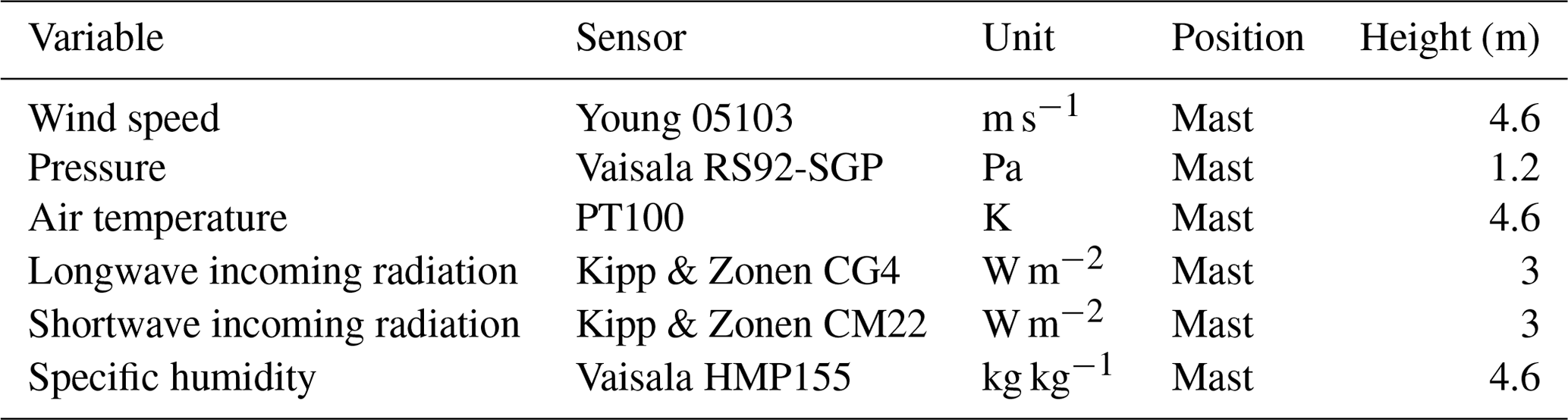
Data describing the local climate were measured at Dome C on a mast equipped with sensors (Genthon et al., 2021), for a 15 d period from 1 to 15 December 2009, the period during which air and surface temperatures are warmest in this region. They constitute a complete data set to feed surface models. The data collected on the mast at a height of 3.3 m are wind direction and speed with a Young anemometer, air temperature in a ventilated shelter with a PT100 probe, and specific humidity. In addition, air pressure was measured by a Vaisala sensor at a height of 1.2 m and measurements of downwelling infrared and visible radiation were made at a height of 3 m with Kipp & Zonen sensors. Periods with missing data were filled with ERA-Interim reanalysis. Due to the lack of precipitation in the period, precipitation rates were set to zero. The above set of variables were averaged every 30 min to generate a continuous forcing over the study period. Table 2 describes the near-surface variables available generated from measurements made at the site and presents some metadata such as instrument type and measurement height.
Table 2Presentation of the forcing data (name, unit, and position on the mast) and instruments used for the measurements.
In situ measurements were available between 8 November 2009 and 1 January 2010 and have enabled to build an atmospheric forcing over a 15 d period starting on 1 December 2009 at 00:00 UTC (i.e., 08:00 LT). Figure 1 shows the temporal evolution of these variables, which constitute the meteorological forcing used for the offline simulations.
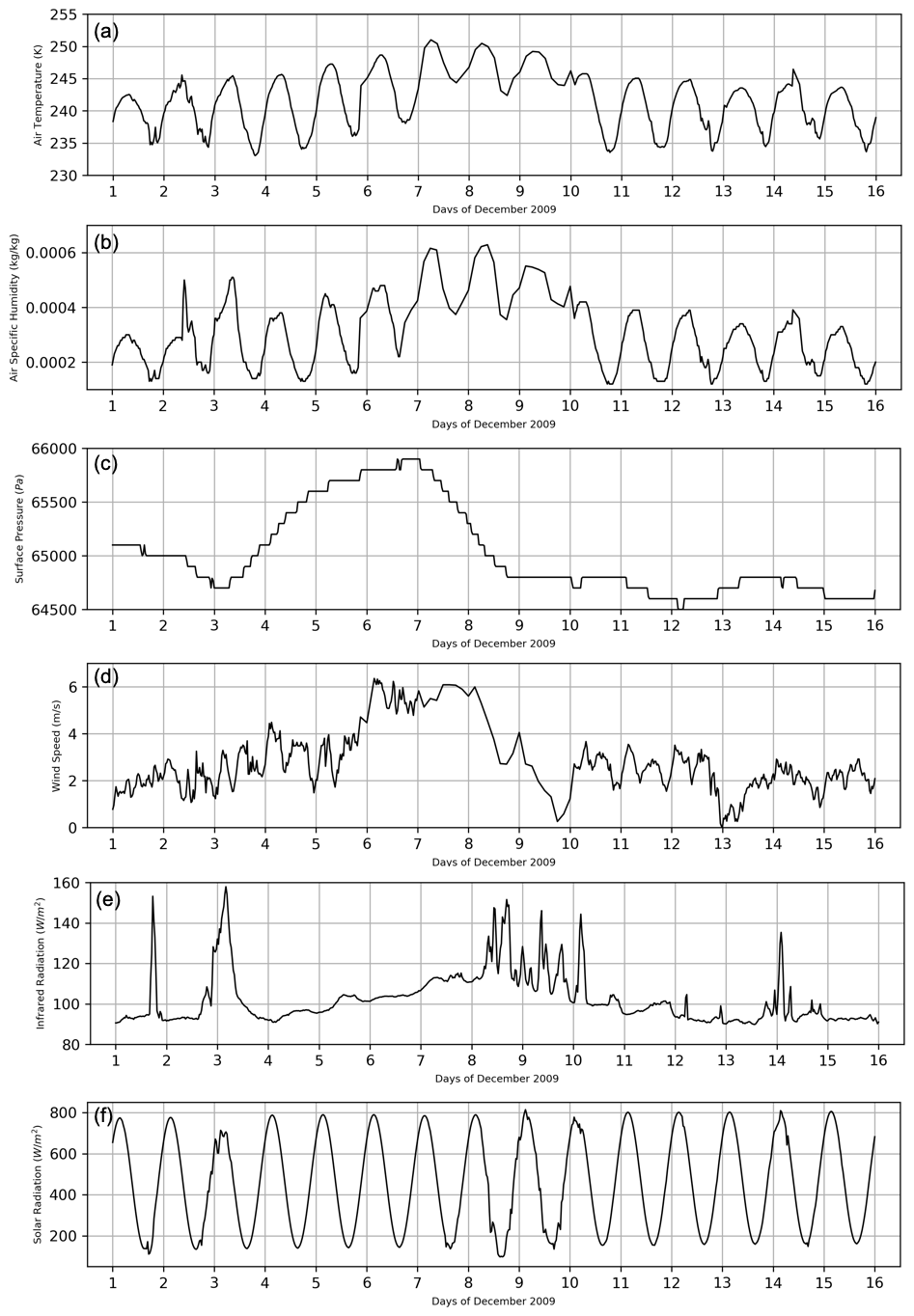
Figure 1Temporal evolution of (a) air temperature, (b) air specific humidity, (c) surface pressure, (d) wind speed, (e) downward infrared radiation, and (f) downward solar radiation for the 15 d period of the offline simulations.
Over the entire period, temperature, air humidity, and wind speed data were missing for days 7–9. The choice was to replace them with data from the ERA-Interim reanalysis (Dee et al., 2011) for these 3 days and not to rescale the measurements. For wind, the measurements showed good agreement with the reanalysis. The reanalysis tends to overestimate the air temperature, especially at night with deviations of about 4 K while during the day this deviation is about 2 K. The low specific humidity is characteristic of very dry air, and the difference between measurements and reanalysis is about 0.1 g kg−1 during the day and night.
During the 15 d, the daily solar radiation varies relatively homogeneously and is characterized by an average diurnal amplitude that oscillates between 180 W m−2 when the sun is low on the horizon and 800 W m−2 when it is at the zenith. Infrared radiation shows a higher temporal variability with low values around 90 W m−2 and higher values around 140 W m−2, corresponding to cloudy periods, visible in particular at the beginning (days 1–3) as well as in the middle (days 8–10) and at the end of the period (day 14). The effect of clouds is also noticeable on the solar radiation time series. The period is also characterized by a strengthening of the surface wind, from 2 to 6 m s−1, associated with an increase in atmospheric pressure (days 5–8). This dynamic effect leads to an increase in specific humidity, related to the arrival of clouds, and an increase in air temperature, probably related to increased mixing in the lower layers or advection effects and a limitation of atmospheric stability and thermal inversion at the surface.
2.4 Evaluation data
Surface and snowpack measurements were used to evaluate the models. Satellite measurements of surface temperature from the Moderate-Resolution Imaging Spectroradiometer (MODIS) and the Infrared Atmospheric Sounding Interferometer (IASI) sensor complemented the continuous measurements from the Baseline Surface Radiation Network (BSRN). Figure 2 shows the measurements from these sensors over the 15 d period.
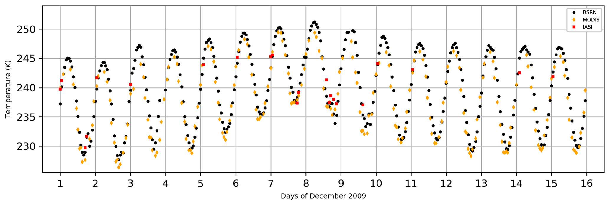
Figure 2BSRN (black dots), MODIS (orange diamonds), and IASI (red squares) observation of surface temperature.
In addition, measurements of the snow temperature profile, made by the Institute for Environmental Geosciences, enabled the characterization of the thermal structure of the snowpack and evaluation of the most sophisticated models with a multilayer vertical discretization (Brucker et al., 2011). The first temperature probe was installed on 26 November 2006 at 10 cm in the snow and the deepest at 21 m. Over time snow was carried by the wind and accumulated on the measurement area. An annual accumulation of 8 cm per year is estimated at Dome C (Genthon et al., 2016; Picard et al., 2019), which corresponds in December 2009 to an accumulation of 23 cm of snow and therefore the first measurement in the snow corresponds to a depth of 33 cm. For the 2 weeks studied, a number of temperature measurements were missing in the snowpack. In particular, the period from 7 to 11 December 2009 was missing and the choice was made to fill it in to study the progression of the diurnal thermal wave in the snowpack over time and its representation in the multilayer models.
The gap-filling method is based on the simulation with the detailed multilayer model CROCUS, for which we consider that the temporal variability of the temperature in the snowpack is well simulated. Indeed, this model has already been evaluated by Brun et al. (2011) over the Antarctic plateau and had simulated the snowpack well. The CROCUS model configuration chosen in this study replicates that used by Brun et al. (2011). Details of the gap-filling method are presented in Appendix A. Figure 3 shows the temperature of each snow layer to a depth of 423 cm (gap filling is performed to a depth of 21 m in the snowpack, combining measurements (black) and data from CROCUS (orange)).
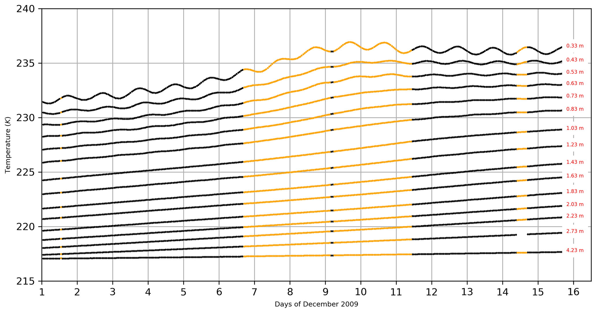
Figure 3Temperature measurements in the snowpack as a function of depth. The black dots represent the in situ measurements and the orange dots are the data reconstructed with the CROCUS model.
Turbulent flux measurements by the eddy correlation are performed at high frequency (10 Hz) (Vignon et al., 2017b) at Dome C on an instrumented mast. The reconstruction of turbulent surface fluxes is a very complex exercise at Dome C, in particular that of the latent heat flux of evaporation and sublimation, because the environmental conditions are extreme and the air is particularly dry. Scientists who have made measurements at Dome C have confirmed that comparisons of latent heat fluxes to simulations are not completely relevant because of the large uncertainty in the measurement. However, we wanted to compare the simulated fluxes with the observations, even if the latter were questionable, because it was an additional way to characterize the variability of the simulations. At this time of the year, some convection is observed, and during “daytime” (i.e., when the sun is high above the horizon), although weak, the sensible heat fluxes are positive, that is, with the sign convention used, there is an energy transfer from the surface to the atmosphere. The sensible heat fluxes for the days of 11 and 12 December 2009 and the following half day were averaged at the hourly time step to be compared with the outputs of numerical simulations.
3.1 Variability of surface parameters
This section aims to show the variability of the surface parameters of the different models, and how they evolve during the simulation, when they are not fixed, as is the case, for example, for the surface broadband albedo. As we will see, the choice of surface parameters is crucial to simulate the surface energy balance with sufficient accuracy. Tables 3–5 give for each model the values or ranges of variation of the surface parameters during the simulation for XP0, calibrated XP0, and XP1, respectively. In Table 3, the albedos are close and represent well a reflective medium like snow. The albedo is a bit larger in GDPS4 and the snow surface will tend to reflect more solar radiation during the day compared with the other constant albedo models. If we consider a radiative flux of 800 W m−2 at the maximum of the day, a surface with an albedo of 0.83 leads to a net solar energy balance of 136 W m−2, while it will be 160 W m−2 for an albedo of 0.80. On the other hand, at night the minimum solar radiation is about 200 W m−2 and the net balance will be 34 and 40 W m−2 for albedos of 0.83 and 0.80, respectively.
Table 3Range of variation of model surface parameters for XP0. The values in square brackets indicate the values taken by a parameter when it is calculated by the model, while the single values are fixed during the simulation.
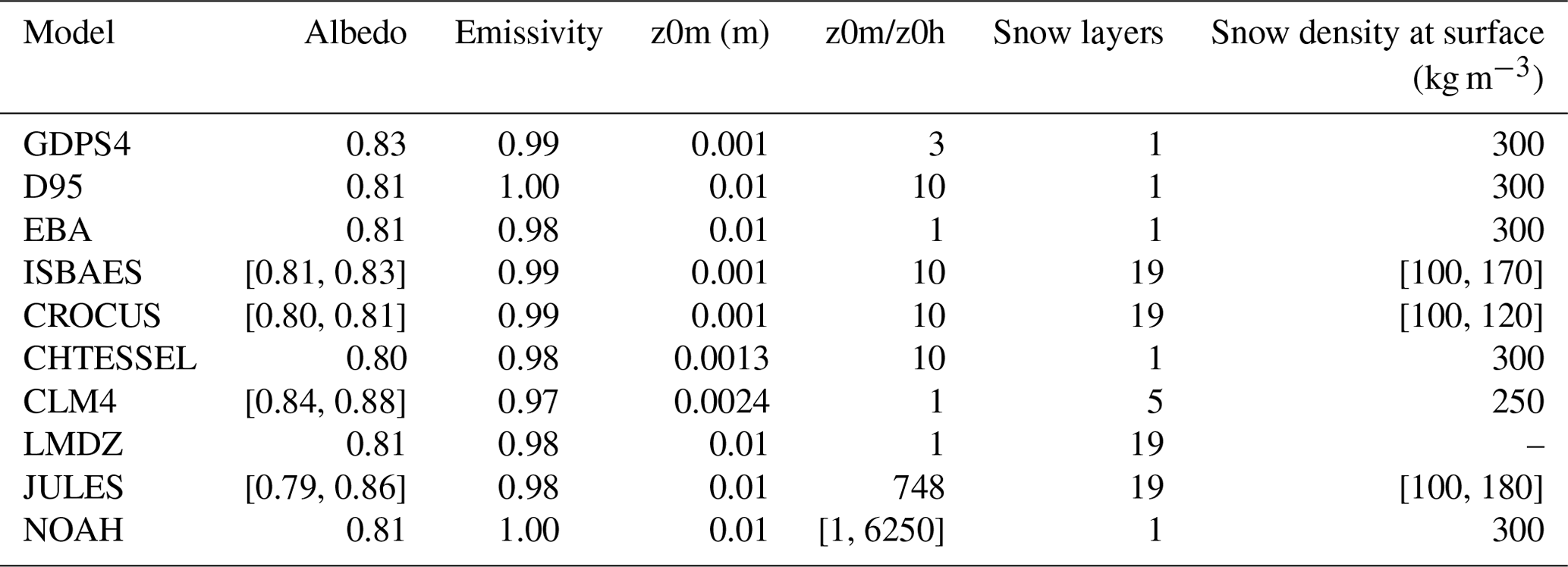
Table 4Range of variation of model surface parameters for calibrated simulations. The values in square brackets indicate the values taken by a parameter when it is calculated by the model, while the single values are fixed during the simulation.
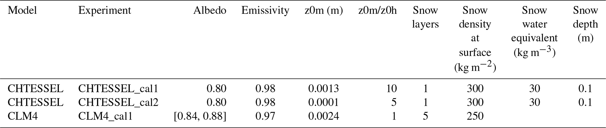
Table 5Range of variation of model surface parameters for XP1. The values in square brackets indicate the values taken by a parameter when it is calculated by the model, while the single values are fixed during the simulation.

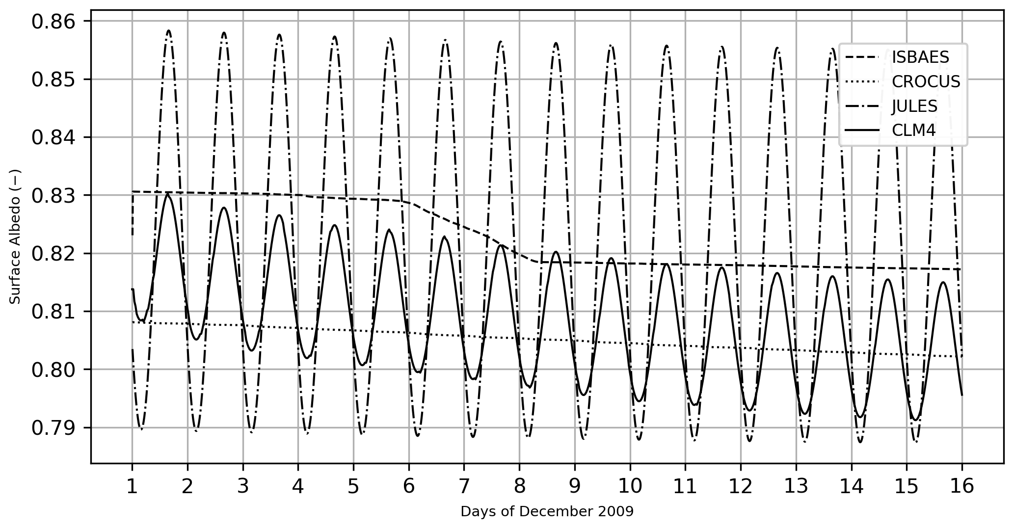
In contrast, Fig. 4 shows the modeled broadband albedos in the four models that model the albedo as a function of the age of the snow, which becomes denser under the effect of wind and compaction. Two of the models, JULES and CLM4, also consider the variation of albedo as a function of the zenith solar angle. We can see a great disparity in the albedos used. In particular, the daytime albedo of JULES (0.79) is lower than the others with a consequence of a stronger warming of the surface. Overall, there is a decrease of about 1 % in the albedo value during the 15 d period. The ISBAES model has a larger albedo at the beginning of the simulation; it undergoes a more marked decrease between days 6 and 8. During this period, there is an increase in air temperature and humidity associated with an intensification in surface wind, which makes the snow denser on the surface. There is also a linear decrease in albedo, which is related to the nature of the model, which redistributes prognostic variables such as snow enthalpy to the snowpack thickness at each time step. In general, the average thickness of the grains increases over time and decreases the albedo. The more significant decrease may be related, we believe, to a more pronounced increase in grain size due to the layer averaging effect. For the CROCUS model, there is a steady decrease in albedo over the period corresponding to the snow aging effect in connection with the steady increase in grain size and there is no impact of the wind intensification on albedo.
The second surface parameter playing an important role in the energy balance is the roughness length. Indeed, dynamic (z0) and thermal (z0h) roughness modulate the surface fluxes of momentum and sensible and latent heat. Vignon et al. (2017a) studied the variations of z0 from measurements at Dome C from which z0 was calculated using the Monin–Obukhov (1954) stability theory (MOST hereafter). They showed that the dynamic roughness varies between 0.01 and 6.3 mm for measurements made between January 2014 and February 2015 (average value of 0.56 mm) and that the value of z0 depends on the wind direction: z0 is lower when the wind is aligned with the sastrugi, surface erosion patterns created by the wind. If it is difficult to estimate the dynamic surface roughness, the determination of the thermal roughness is also subject to many uncertainties (Andreas, 2002) and most often the models use a thermal roughness proportional to the dynamic roughness. This is the case for the models here except for NOAH whose z0h is derived by a seasonally varying formulation dependent on the seasonal cycle of green vegetation fraction (Zheng et al., 2012). The calculation of surface fluxes is based on, for many models, MOST which describes the influence of stability and roughness on turbulent exchange coefficients, the latter decreasing with increasing stability (Blyth et al., 1993). In Antarctica, turbulent flux exchange coefficients are low because the atmosphere is mostly stable and roughness is low (Deardorff, 1968). Surface roughness can also impact albedo by altering the effective zenith solar angle (Hudson et al., 2006) and produce shadow zones at the surface (Leroux and Fily, 1998).
3.2 Surface temperature
The surface temperature directly influences the ambient air temperature and is itself directly influenced by the surface energy budget. In summer, the diurnal cycle of the surface temperature is driven to the first order by the diurnal cycle of the solar radiation, which itself depends on the diurnal cycle of the solar zenith angle. At “night” (i.e., when the sun is low above the horizon), the zenith solar angle is low and the surface albedo is maximum. The infrared thermal radiation deficit then exceeds the solar radiation gain and cools the surface. During the day, it is the opposite which occurs, i.e., the solar zenith angle is high while the albedo decreases inducing a heating of the surface by the solar radiation. The simulation of the surface temperature by the different models is a key point of our study. We were interested in the diurnal cycle of surface temperature over the 15 d of simulations, in particular the dispersion of all models but also their ability to simulate very cold diurnal cycles with strong thermal amplitudes. The simulations were compared to the available in situ and satellite measurements. Figure 5 shows the time series of modeled surface temperatures (gray lines), on which the in situ measurements of the BSRN (black dots) and satellite measurements from MODIS (orange dots) and IASI (red dots) are also shown. Overall, the models are able to simulate the surface temperature quite well. However, there are strong disparities between some simulations, during both day and night, where the largest temperature differences can exceed 10 K. All models overestimate the temperature at night on 7 and 8 December, which correspond to missing data filled with ERA-Interim which is warmer than the locally observed temperatures.
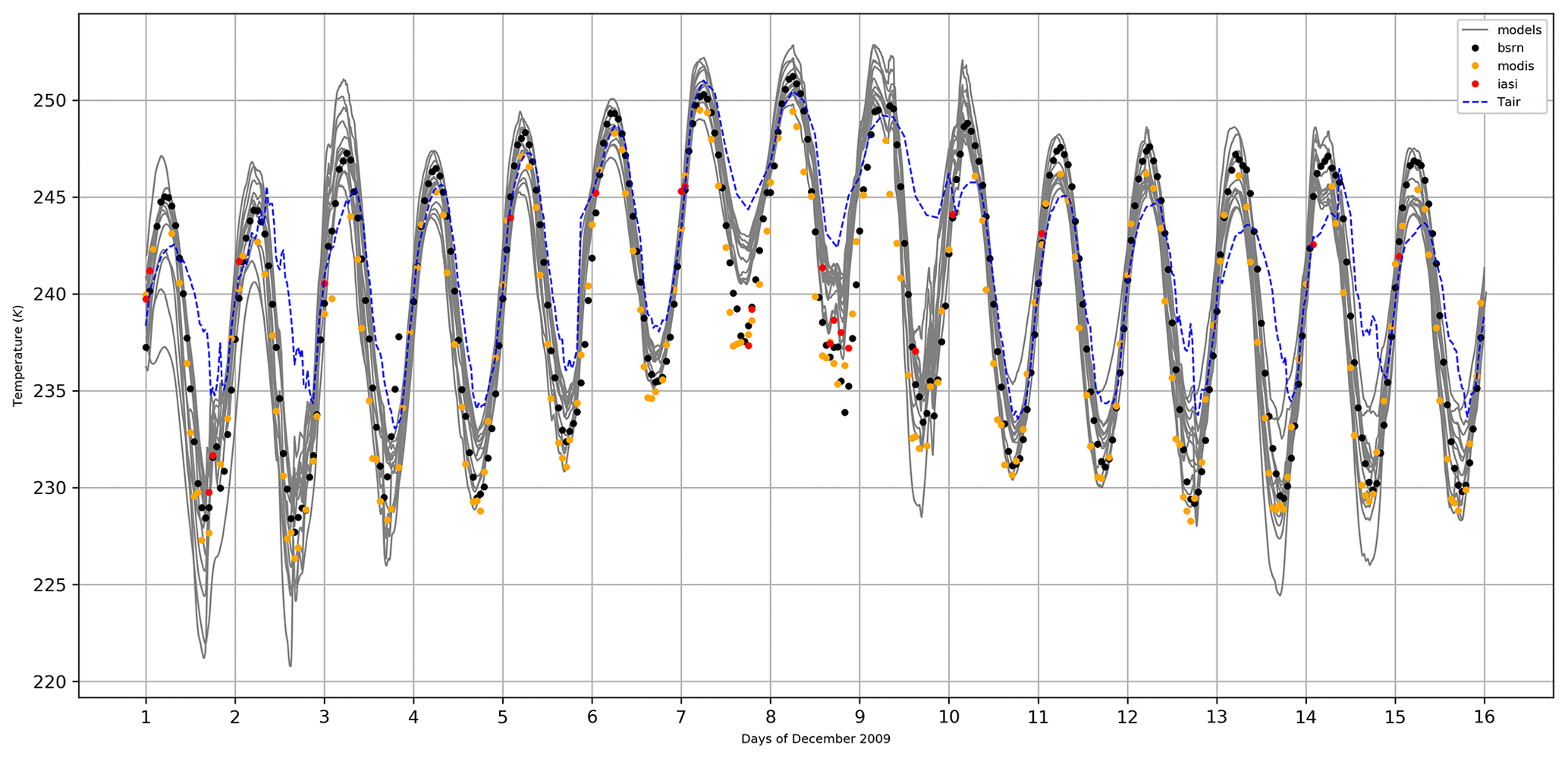
Figure 5Temporal evolution of the surface temperature observed by BSRN (black dots), MODIS (orange dots), and IASI (red dots), simulated by the different models (gray lines), and of the air temperature (dashed blue line).
To better account for the behavior of the different models with respect to the observations, a probability distribution function (PDF) was computed for each model and for the BSRN observations, and each PDF was fitted by a cubic splines. MODIS and IASI observations were not used in this analysis because their number was insufficient for a robust statistical processing. In Fig. 6, the observed surface temperature PDF is indicated by the black dots, fitted by a cubic function (dashed line).
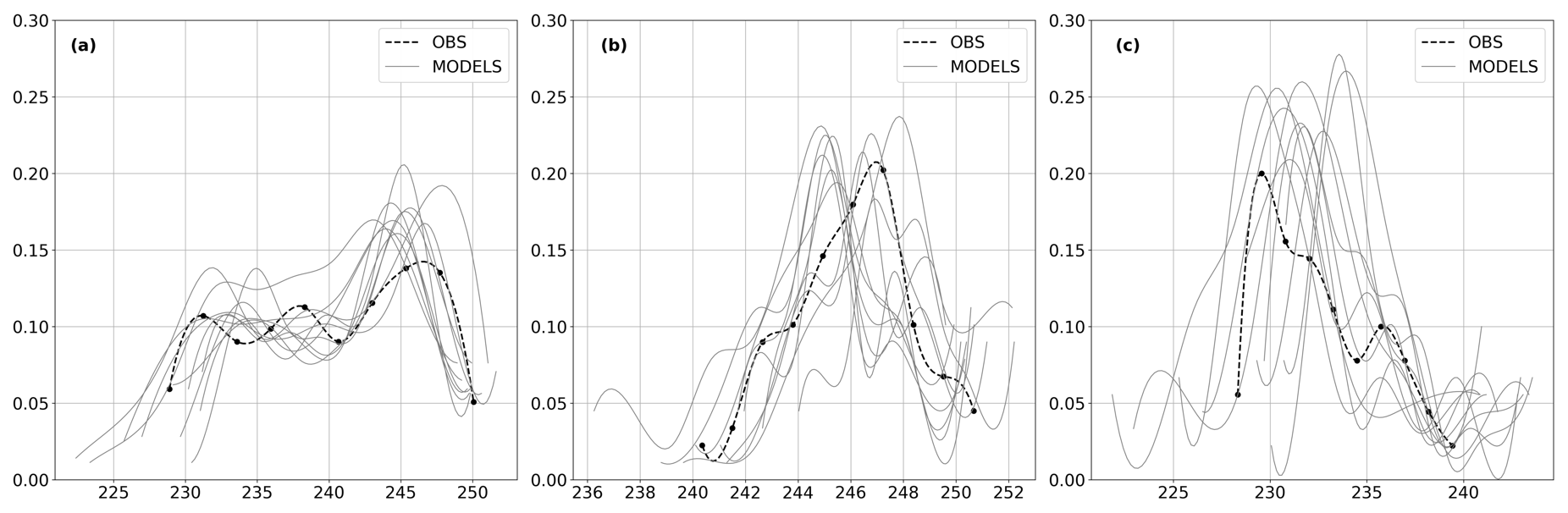
Figure 6Probability density of observed (dashed black line) and modeled (solid gray lines) surface temperature for (a) all temperatures, (b) daytime (09:00–15:00 LT) temperatures, and (c) nighttime (21:00–03:00 LT) temperatures.
Over the whole period (Fig. 6a), we notice a trimodal distribution from observation and models that tend to underestimate the maximum temperature and overestimate the minimum temperature. The decomposition into day (Fig. 6b) and night (Fig. 6c) time ensembles better illustrates these behaviors. Daytime is defined as the period 00:00–06:00 UTC (09:00–15:00 LT), while nighttime is defined as 12:00–18:00 UTC (21:00–03:00 LT). In particular, during the day, most of the models have a distribution fairly close to that of the observation but with a tendency to be about 2 K cooler. Some models have a distribution closer to that of the observation. At night, two peaks appear which correspond to minimum temperatures (around 230 K) and the second peak around 236 K which also corresponds to minimum temperatures but in warmer air between days 6 and 10. The model distributions are more scattered at night. If the models manage to reproduce the nighttime cooling, many of them tend to overestimate the surface temperature, from 2–3 K for some to 5 K for others. Figure 7 shows the statistical behavior of all the simulations performed, calculated at hourly intervals, in terms of bias and root mean square deviation (RMSD). Indeed, each contributor was allowed to send the results of several realizations of the proposed simulation. On the x axis of this figure we find the name of an experiment, composed of the name of the model and a suffix corresponding to the test performed. Note that the experiments with the extension “_new” correspond to the rerun which is described below.
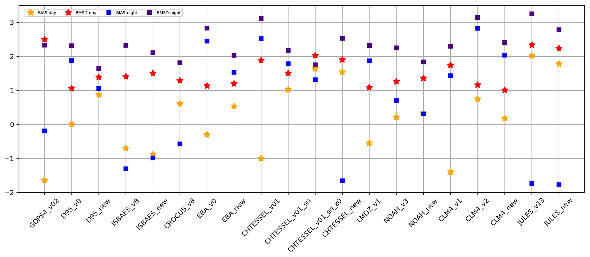
Figure 7Statistical scores (BIAS and RMSD) during the day and night for the simulations performed for each model configuration.
3.3 Impact of the rerun on the surface temperature simulations
The conditions imposed for the rerun show that the daytime RMSD varies only slightly between XP0 and XP1 with sometimes smaller errors for XP0 and other times for XP1 as shown in Table 6.
Table 6Impact of rerun on BIAS and RMSD of model surface temperatures.
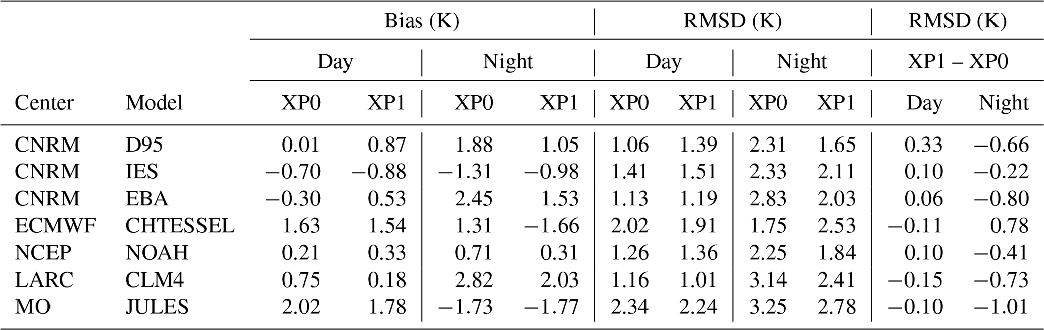
On the other hand, the RMSD is significantly improved at night for almost all models with improvements up to 1K. The majority of the models have a smaller daytime bias than the nighttime bias for both XP0 and XP1, confirming the greater difficulty of the schemes in representing the more stable conditions at night. This can be attributed to the snow scheme (in particular albedo, emissivity, thermal coefficient of the snow, and grain size) or to the parameterization of the turbulent fluxes at the surface–atmosphere interface (dynamic and thermal roughness lengths involved in the calculation of the turbulent exchange coefficients, as well as air stability criterion), in addition to the surface temperature itself depending on the albedo, emissivity, and thermal coefficient of the snow. Moreover, XP1 type experiments tend to show larger biases, especially during the day but not for all models, and tend to decrease them at night. Therefore, in order to propose a comparison of all the models, we decided to retain the best simulation of each model, performed in the XP0 framework. Each model is therefore evaluated separately from the in situ observations, and it is also a challenge of this intercomparison to learn from the different models to see what could be improved. To do this, a comparison of the simulated and observed time series was carried out by separating the night periods, i.e., corresponding to the hours between 12:00 and 18:00 UTC, from the day periods between 00:00 and 06:00 UTC. This choice was motivated by the very strong diurnal amplitude at Dome C and the need to avoid error compensation during bias calculations. Biases, root mean square error (RMSE), and correlations were calculated on hourly data considering for each observation the closest simulation time. The results obtained are summarized in Taylor diagrams presented in Fig. 8.
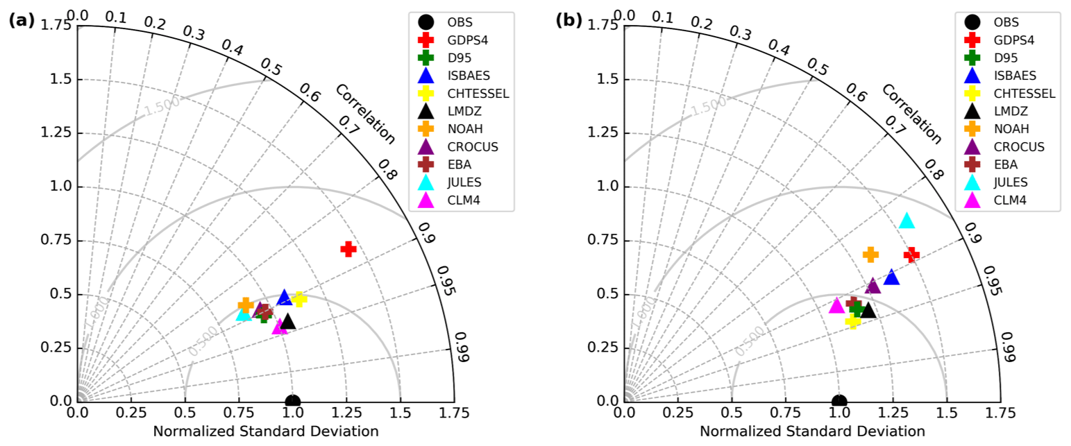
Figure 8Taylor diagram comparing the surface temperature scores of the different models (a) during the day and (b) at night. The crosses correspond to single-layer models and the triangles to multilayer models.
As a result, most of the models manage to represent the surface temperature during the day, except for the GDPS4 model which presents a higher error than the others. On the other hand, the results at night confirm the distributions of the PDFs, with a greater dispersion, a correlation that is fairly homogeneous and high around 0.9, and a root mean squared error that varies from 0.4 K (CHTESSEL) to 1 K (JULES). It should be noted that the single-layer models (D95, CHTESSEL, and EBA) sometimes have better results than the more sophisticated models which have to represent more physical processes, such as the evolution of albedo with time and the increase in snow density by compaction, among others. The advantage of these simple models is that they are able to represent well the exchanges at the surface–atmosphere interface thanks to adapted surface parameters, such as the albedo and the heat transfer coefficient in the snow.
3.4 Sensible and latent heat flux
In this section, model comparisons to turbulent sensible and latent heat flux measurements, for the original versions of the models (XP0), are presented. The estimation of the contribution of sensible and latent heat fluxes to the surface energy balance is based, for all the models considered, on MOST, which describes in particular the influence of atmospheric stability and surface roughness on the variability of the exchange coefficient used for the calculation of the fluxes. Indeed, the sensible and latent heat fluxes, expressed in their bulk form, are proportional to the wind speed multiplied by the vertical gradient of temperature and specific humidity between the surface and the air, respectively. For sensible heat flux, the proportionality coefficient is the turbulent surface exchange coefficient multiplied by the air density and the heat capacity. An increase in air stability induces a decrease in the exchange coefficient (Kondo, 1975; Blanc, 1985; Blyth et al., 1993). Thus, in Antarctica, the stable boundary layer and low surface roughness induce very low turbulent fluxes and exchange coefficients (Deardorff, 1968).
Eddy covariance measurements were performed during the 2 months, December 2009 and January 2010, at Dome C and have characterized the sensible and latent heat flux for 2.5 consecutive days, with the first day, 11 December 2009, corresponding to the golden day as defined in the experimental protocol of the GABLS4 intercomparison exercise. Figure 9 compares Qh, the hourly sensible heat flux simulated by the different models, with the observations. First of all, the graph shows two clearly distinct classes, corresponding on the one hand to the night with observed flux values between −2.5 and +2.5 W m−2 and on the other hand to the day with observed values between 2.5 and 15 W m−2. At night, turbulence is lower than during the day, partly because the wind modulus is lower, but also because the air density is higher and reduces the air vertical motion. Indeed, for the days considered, the minimum wind speed observed is about 2 m s−1 at night and 3.5 m s−1 during the day. Moreover, the radiation balance is negative at night, leading to a cooling of the surface temperature, and positive during the day, thanks to the incident solar radiation that heats the snow. The simulated sensible heat fluxes show a bimodal behavior, with symmetrical and opposite values for day and night. During the day, the models simulate sensible heat fluxes between 5 and 40 W m−2 and at night between −40 and −5 W m−2. The assumed overestimation of sensible heat fluxes under stable conditions is a long-standing feature of the models, although it may prevent larger biases in the surface temperature (King and Connolley, 1997).
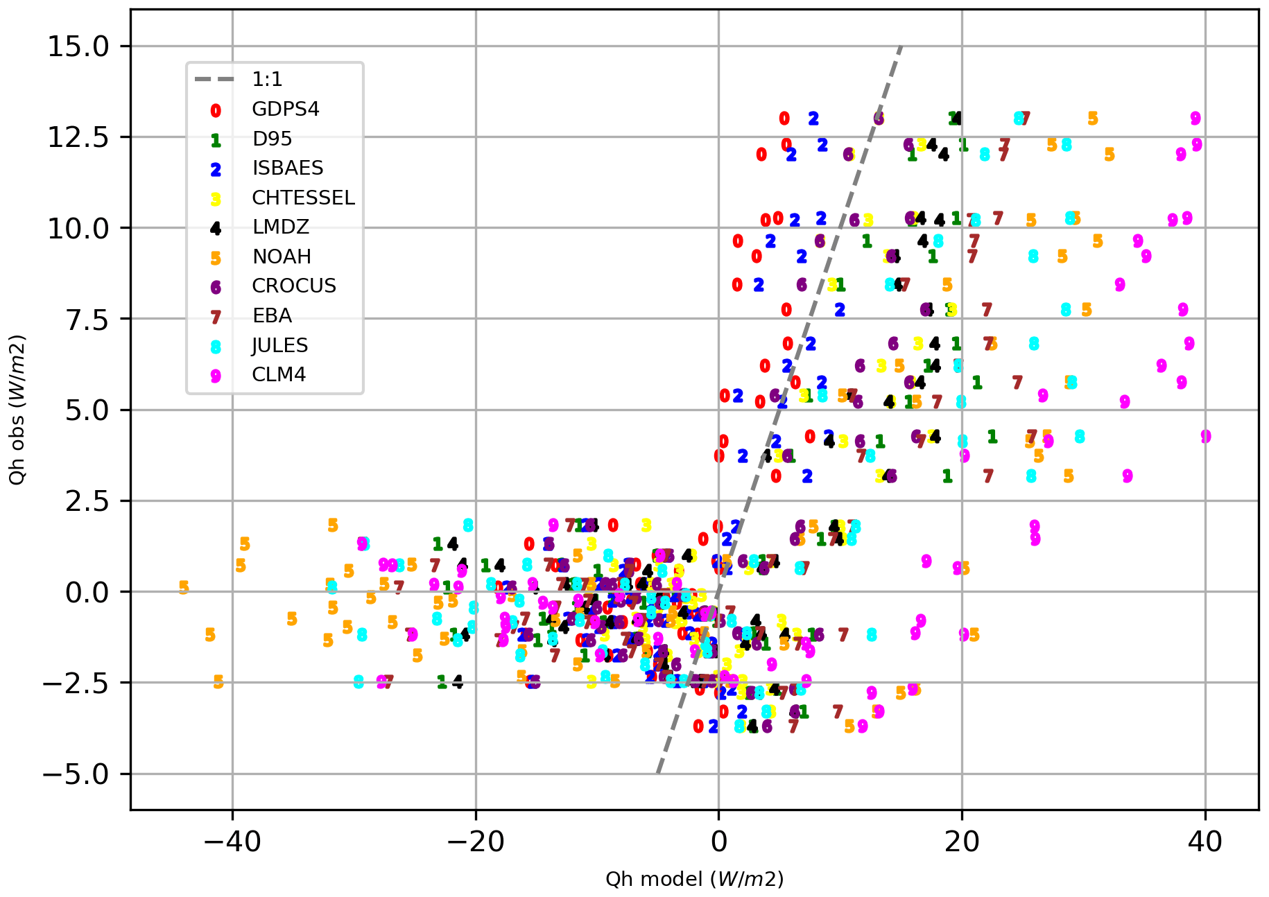
Figure 9Scatterplot of sensible heat flux simulated (x axis) and measured (y axis). The dashed gray line represents the 1:1 line.
In the same way, Fig. 10 allows us to compare Qle, the hourly latent heat flux simulated by the different models, with the observations. The first lesson that can be learned from this plot is that for all models except NOAH, the latent heat fluxes are lower than the values measured by the eddy covariance. Second, there is a separation around 5 W m−2 for the observed Qle which corresponds to daytime for the higher values and nighttime and day/night transition for the lower values. At night, the modeled values are low between −2 and +4 W m−2 and during the day between 2 and 5 W m−2 for most models except for CLM4 and NOAH which exhibit higher values. Figures 9 and 10 compare Qh and Qle, the hourly sensible and latent heat flux, respectively, simulated by the different models, with the observations. We see at first that the measured latent heat flux is abnormally high. Indeed, as shown by King et al. (2006), this flux can only be of the order of a few W m−2 at Dome C, and that the closure of the energy balance has a high uncertainty. Thus, the reconstruction of heat fluxes from the eddy covariance measurements is likely to be subject to error, and comparisons made here should be done with caution.
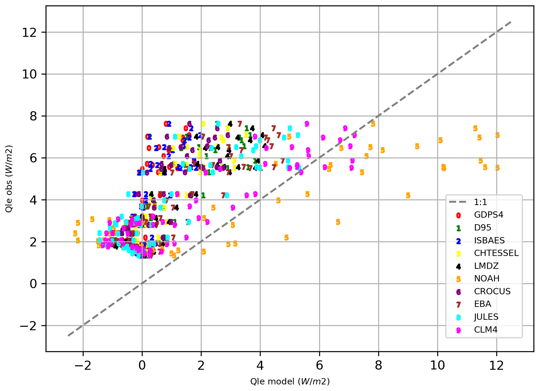
Figure 10Scatterplot of latent heat flux simulated (x axis) and measured (y axis). The dashed gray line represents the 1:1 line.
We are now interested in the variations of Qh for the different models. The measured sensible heat flux is written:
where ρ is the air density, Cp is the heat capacity at constant pressure, and is the average correlation between the vertical velocity and potential temperature fluctuations. Qh is modeled by its Bulk form as follows:
where Ch is the turbulent exchange coefficient, Ua and Ta are the wind speed and air temperature, respectively, and Ts is the temperature at the snow surface.
Each model solves its own energy balance and calculates in particular the surface temperature, a variable which is at the heart of the resolution of this balance. The variability of the models in terms of surface temperature will directly impact the variability in terms of sensible heat flux. Similarly, the atmospheric conditions near the surface, i.e., temperature and wind speed, modulate the calculation of the Qh flux. Equation (6) also involves Ch which depends on the dynamic and thermal roughness lengths as well as the stability of the air characterized by the bulk Richardson number Ri, except for the GDPS, CLM4, and NOAH models, for which the calculation of Ch is iterative and based on Monin–Obukhov's theory.
The bulk Richardson number is expressed as:
where g is the acceleration of gravity, 〈T〉 the average virtual temperature, and Δθ and ΔU the gradients of virtual potential temperature and wind speed of the considered layer of thickness Δz. The very low humidity of the air allows to assimilate the average virtual temperature and the virtual potential temperature to the average temperature and the average potential temperature.
Figure 11a shows how Ch, normalized by its value at neutrality (i.e., when Ri=0), varies as a function of Ri for all models that provided values. that the curves do not collapse into a single universal one, and which highlights the fact that most models have tuned their stability function from the universal one. We note a strong dispersion in the representation of the normalized exchange coefficient depending on the model. Values can be twice as large in some cases, such as in convective conditions when Ri is equal to −3. On the other hand, the values are very low for the stable atmosphere cases, i.e., when Ri is positive, which is in good agreement with weaker turbulent exchanges or even almost zero in these conditions. To highlight the disparities in the Ch coefficient, the temporal evolution of Ch has been plotted in Fig. 11b for all models, as well as the value of this coefficient calculated from the observations. Figure 11b shows that Ch is simulated rather well for low turbulence conditions (low Ch) but is overestimated for the GDPS4, CLM4, and NOAH models. On the other hand, when the turbulence increases (13 December), these models simulate Ch quite well; however, the variability of the simulated Ch is then much greater.

Figure 11Turbulent exchange coefficient for heat Ch normalized by its value under neutral conditions as a function of the Richardson number (a), and Ch as a function of time (b).
3.5 Temperature profile in the snow
Some of the models are multilayered and simulate the evolution of the profile of the variables that characterize the snowpack (density, temperature, enthalpy, etc.). Thus, the JULES, ISBAES, CROCUS, and LMDZ models have an identical vertical discretization of the snowpack in 19 layers as recommended by the experimental protocol, while CLM4 has a discretization in 5 layers. Few observed data are available to make comparisons with the simulations, except for snow temperature. The snow temperature profiles of the multilayer models were therefore evaluated over the 15 d period by comparison with measurements made at different depths. In order to make an identical comparison for all models, a vertical interpolation of the observed and simulated profiles was performed on a fine grid with a resolution of 1 cm. The first statement concerns the results of CLM4, which are very different from the other models, with an unrealistic tendency to overheat the snow. (The results are therefore not presented here.) Figure 12 shows the deviations in the temperature profiles from observations over time. (The temporal evolution of the observed temperature profile is shown in Fig. A2 in Appendix A.)
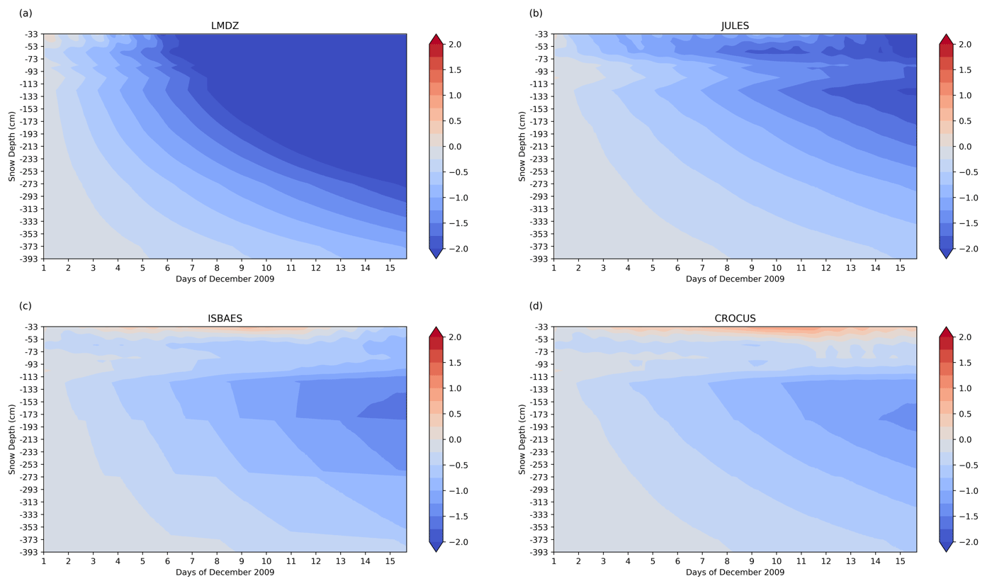
Figure 12Temporal evolution of deviations from observations of the temperature profile in snow.
It can be seen that the initialization of the vertical temperature profile is identical and correctly configured for all four models. The temporal evolution differs significantly from one model to another, except between ISBAES and CROCUS which have a large number of parameterizations in common. The LMDZ model tends to overcool the snowpack and this cooling appears at the surface and propagates into the deeper layers generating a generalized cold bias over the whole snowpack and reaching −2 K. The configuration of the LMDZ model for this intercomparison is particular since the model is not really a snow model but rather a soil model with the characteristics of snow. Sensitivity experiments on the coupled GABLS4 case revealed that the default value of the snow thermal inertia set over Antarctica in LMDZ was way too high (close to a typical pure ice value). This parameter was therefore calibrated to a more realistic value after the GABLS4 exercise, leading to significant improvements of the temperature diurnal cycle (not shown here; see Vignon et al., 2017b). For the remaining three models, similar behaviors can be observed for snow layers deeper than 1 m, but a different response is observed between JULES and the two other models for the layers closest to the surface, between 33 cm and 1 m deep. Indeed, over time JULES tends to generate a cold bias reaching 2 K at the end of the period in the first meter, while ISBAES and CROCUS let heat penetrate more easily and the differences with observations vary between −0.5 and +0.5 K. At the end of the period, CROCUS is the model with the lowest bias, of the order of −1 K at 153 cm, which is a very good score, while this bias is −1.5 and −2 K for ISBAES and JULES, respectively, indicating that these two models also perform well.
The study showed that the simple models performed well as long as the surface albedo and heat capacity were well prescribed. This is a very relevant finding for numerical weather prediction models because not all of them use very sophisticated snow models. Indeed, single-layer models are often preferred because multilayer models represent a non-negligible cost in numerical weather prediction (NWP) models (even if the cost of surface schemes is only a few percentage of the total model cost) and also because they significantly increase the complexity of the data assimilation schemes. However, multilayer models, which are more complex and have more advanced physics, can offer better performance. They are essential to study the internal dynamics of the snowpack and the penetration of the heat wave. One of the key variables for these models is the optical diameter of the snow used to characterize the snow microstructure which modulates the spectral albedo and has a direct impact on all snowpack processes, but unfortunately observations are rare and anyway difficult to use in an NWP context.
It was found that the intercomparison of snow models at Dome C was very valuable in several ways. First of all, the environmental conditions on the Antarctic plateau are extreme and testing the models under these conditions is very beneficial, especially for detecting their limitations. The results showed the good capacity of all models to represent correctly the temporal evolution of the surface temperature. The simplest as well as the most complex models are able to simulate the surface temperature thanks to a good simulation of the energy balance and all the better as the surface parameters are realistic. Indeed, the models are very sensitive to surface parameters such as albedo and surface roughness, and a large part of the intermodel variability comes from the disparity between these parameters in the models. Moreover, complex multilayer models have shown their ability to represent not only the surface exchanges but also the thermodynamics of the snowpack. This aspect is very important when it comes to coupling these surface schemes with the atmosphere, as for example in climate models, which are used to study, among other things, the impact of climate change on the snow cover and ice caps, with particular attention to the ice melting at the poles. This study has largely focused on snow models that are used within global models and have not been specifically optimized for polar conditions. However, it is important to note that work has been done to develop snow and firn models optimized for polar conditions for use in regional NWP and climate models, such as Polar WRF (Hines and Bromwich, 2008), MAR (Agosta et al., 2019), and RACMO2 (van Wessem et al., 2018).
We chose to reconstruct the missing atmospheric forcing data using the ERA-Interim reanalysis data to avoid interpolation of the measurements, which would lead to uncertainty. The magnitude of the temperature difference between ERA-Interim and the measurements over the 15 d period reaches 4 K during the day and 2 K at night. This is a fairly large difference, which was identified by Fréville et al. (2014), who found an overestimation of the turbulent mixing near the surface due to the parameterization of surface fluxes and a too large turbulent exchange coefficient. This was further investigated in Dutra et al. (2015), and the effective snow depth was even more important than the sensible heat flux.
However, snow has a low heat capacity and therefore the duration of the impact of such a difference was small. Other simulations (not shown) to study the impact of spin-up on heat wave penetration also confirm this. And this is important because the golden day selected for GABLS4 and the coupled surface–atmosphere simulations follows this period of missing data.
Surface flux comparisons are also subject to debate. Indeed, on the one hand, measurements by eddy covariance present large uncertainties, and on the other hand, the calculation by models, using the MOST theory, is not necessarily adapted to very stable conditions. Indeed, the surface parameterizations in stable cases have long been deficient and atmospheric models have had difficulty in representing cases of high stability. For example, in this study, the turbulent exchange coefficient for heat is overestimated by all models compared with that diagnosed from observations (not shown). However, these measurements, even if they are subject to error, are invaluable in understanding the processes and in the possibility of comparing the results of the models with observations. Moreover, these observations are rather rare, and having more measured and quality-controlled data would be great progress. In the end, the temperatures simulated by these forced models are relatively good, and an evaluation of the models in coupled mode is the logical continuation of this work, which also requires good-quality observation data sets.
We consider the observed snow temperature profiles at two distinct times t1 and tn and the open time interval ]t1,tn[ during which the observations are missing. Moreover, for each snow layer, we know the temperatures simulated by CROCUS for each time of the interval [t1,tn] and we calculate the temperature TOBS′(tk) which would be observed at time tk for a given layer if the temporal evolution of the temperature profile were that of CROCUS. We calculate the value D(tk) to be added or subtracted at time tk to the CROCUS temperature to find the observed value:
The sign prime indicates that it is an interpolated value and not the real observed value. For this, it is assumed that for each snow layer, D(tk) varies linearly between D(t1) and D(tn) which verify:
and
where TOBS(t1), TOBS(tn), TCRO(t1), and TCRO(tn) are the values of the temperatures observed and simulated by CROCUS at times t1 and tn for the layer j considered. It follows that:
where
Figure A1 highlights the principle of the observed temperature reconstruction method.
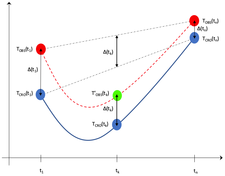
Figure A1Schematic diagram of the method of filling in the missing values observed from a numerical simulation with the CROCUS model.
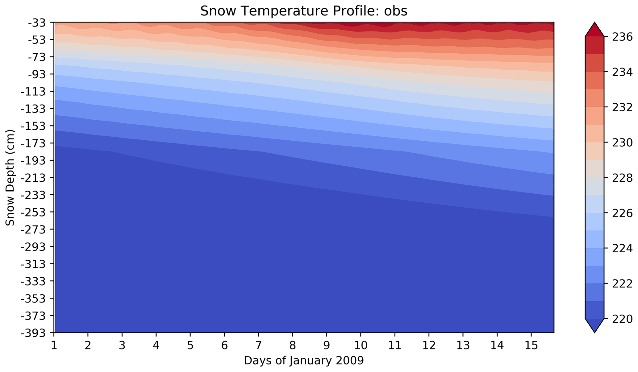
Figure A2Temperatures in snow as a function of time for the 15 d period in December 2009, interpolated to a fine vertical grid.
Figure A2 shows the temperature profile in the snowpack reconstructed from the measurements and completed by the temperatures interpolated by using the time variability of the simulated CROCUS temperatures for the different layers using the algorithm described above. This field was then interpolated on a 1 cm resolution vertical grid in order to make comparisons with the detailed models which do not have the same vertical discretization.
The data used in the figures, i.e., forcing data, simulations results, observations, and the Python scripts used to process the data, can be downloaded here: https://doi.org/10.5281/zenodo.5814726 (Le Moigne, 2022).
PLM and EB designed the experiments, and AC, AZ, ED, EV, IS, JME, PLM, and WZ carried them out. WM and OT provided the in situ measurements and surface fluxes. PLM prepared the manuscript with contributions from all co-authors.
The contact author has declared that neither they nor their co-authors have any competing interests.
Publisher's note: Copernicus Publications remains neutral with regard to jurisdictional claims in published maps and institutional affiliations.
The first author warmly thanks Eric Brun for the support given to this study and for the configuration of the CROCUS model, and Eric Brun, Aaron Boone, and Bertrand Decharme for the constructive discussions on the snow models.
This paper was edited by Masashi Niwano and reviewed by Richard L. H. Essery and John King.
Agosta, C., Amory, C., Kittel, C., Orsi, A., Favier, V., Gallée, H., van den Broeke, M. R., Lenaerts, J. T. M., van Wessem, J. M., van de Berg, W. J., and Fettweis, X.: Estimation of the Antarctic surface mass balance using the regional climate model MAR (1979–2015) and identification of dominant processes, The Cryosphere, 13, 281–296, https://doi.org/10.5194/tc-13-281-2019, 2019.
Andreas, E. L.: Parametrizing scalar transfer over snow and ice: a review, J. Hydrometeorol., 3, 417–432, https://doi.org/10.1175/1525-7541(2002)003<0417:PSTOSA>2.0.CO;2, 2002.
Armstrong, R. L. and Brun, E.: Snow and Climate: Physical Processes, Surface Energy Exchange and Modeling, Cambridge University Press, ISBN 9780521854542, 2008.
Bazile, E., El Haiti, M., Bogatchev, A., and Spiridonov, V.: Improvement of the snow parametrisation in ARPEGE/ALADIN, in: Proceedings of SRNWP/HIRLAM Workshop on surface processes, turbulence and mountain effects, 22–24 October 2001, Madrid, HIRLAM 5 Project, 14–19, 2002.
Bazile, E., Couvreux, F., Le Moigne, P., Genthon, C., Holtslag, A. A. M., and Svensson, G.: GABLS4: An intercomparison case to study the stable boundary layer over the Antarctic Plateau, Global Energy and Water Exchanges News, 24, https://www.gewex.org/gewex-content/files_mf/1432213914Nov2014.pdf (last access: 2 June 2022), 2014.
Best, M. J., Pryor, M., Clark, D. B., Rooney, G. G., Essery, R. L. H., Ménard, C. B., Edwards, J. M., Hendry, M. A., Porson, A., Gedney, N., Mercado, L. M., Sitch, S., Blyth, E., Boucher, O., Cox, P. M., Grimmond, C. S. B., and Harding, R. J.: The Joint UK Land Environment Simulator (JULES), model description – Part 1: Energy and water fluxes, Geosci. Model Dev., 4, 677–699, https://doi.org/10.5194/gmd-4-677-2011, 2011.
Blanc, T. V.: Variation of Bulk-Derived Surface Flux, Stability, and Roughness Results Due to the Use of Different Transfer Coefficient Schemes, J. Phys. Oceanogr., 15, 650–669, 1985.
Blyth, E. M., Dolman, E. J., and Wood, N: Effective resistance to sensible- and latent-heat flux in heterogeneous terrain, Q. J. Roy. Meteor. Soc., 119, 423–442, https://doi.org/10.1002/qj.49711951104, 1993.
Boone, A. and Etchevers, P.: An Intercomparison of Three Snow Schemes of Varying Complexity Coupled to the Same Land Surface Model: Local-Scale Evaluation at an Alpine Site, J. Hydrometeorol., 2, 374–394, https://doi.org/10.1175/1525-7541(2001)002<0374:AIOTSS>2.0.CO;2, 2001.
Boone, A., Habets, F., Noilhan, J., Clark, D., Dirmeyer, P., Fox, S., Gusev, Y., Haddeland, I., Koster, R., Lohmann, D., Mahanama, S., Mitchell, K., Nasonova, O., Niu, G.-Y., Pitman, A., Polcher, J., Shmakin, A. B., Tanaka, K., van den Hurk, B., Vérant, S., Verseghy, D., Viterbo, P., and Yang, Z.-L.: The Rhône-Aggregation Land Surface Scheme Intercomparison Project: An Overview, J. Climate, 17, 187–208, https://doi.org/10.1175/1520-0442(2004)017<0187:TRLSSI>2.0.CO;2, 2004.
Bosveld, F. C., Baas, P., Steeneveld, G.-J., Holtslag, A. A. M., Wangevine, W. M., Bazile, E., de Bruijn, E. I. F., Deacu, D., Edwards, J. M., Ek, M., Larson, V. E., Pleim, J. E., Raschendorfer, M., and Svensson, G.: The third GABLS intercomparison case for evaluation studies of boundary-layer models, Part B: results and process understanding, Bound.-Lay. Meteorol., 152, 157–187, 2014.
Boussetta, S., Balsamo, G., Beljaars, A., Panareda, A.-A., Calvet, J.-C., Jacobs, C., van den Hurk, B., Viterbo, P., Lafont, S., Dutra, E., Jarlan, L., Balzarolo, M., Papale, D., and van der Werf, G.: Natural land carbon dioxide exchanges in the ECMWF integrated forecasting system: Implementation and offline validation, J. Geophys. Res.-Atmos., 118, 5923–5946, https://doi.org/10.1002/jgrd.50488, 2013.
Bowling, L. C., Lettenmaier, D. P., Nijssen, B., Phil Graham, L., Clark, D. B., El Maayar, M., Essery, R., Goers, S., Gusev, Y. M., Habets, F., van den Hurk, B., Jin, J., Kahan, D., Lohmann, D., Ma, X., Mahanama, S., Mocko, D., Nasonova, O., Niu, G.-Y., Samuelsson, P., Shmakin, A. B., Takata, K., Verseghy, D., Viterbo, P., Xia, Y., Xue, Y., and Yang, Z.-L.: Simulation of high-latitude hydrological processes in the Torne–Kalix basin: PILPS Phase 2(e): 1: Experiment description and summary intercomparisons, Global Planet. Change, 38, 1–30, https://doi.org/10.1016/S0921-8181(03)00003-1, 2003.
Brucker, L., Picard, G., Arnaud, L., Barnola, J.-M., Schneebeli, M., Brunjail, H., Lefebvre, E., and Fily, M.: Modeling time series of microwave brightness temperature at Dome C, Antarctica, using vertically resolved snow temperature and microstructure measurements, J. Glaciol., 57, 171–182, https://doi.org/10.3189/002214311795306736, 2011.
Brun, E., Martin, E., Simon, V., Gendre, C., and Coleou, C.: An Energy and Mass Model of Snow Cover Suitable for Operational Avalanche Forecasting, J. Glaciol., 35, 121, 333–342, https://doi.org/10.3189/S0022143000009254, 1989.
Brun, E., Six, D., Picard, G., Vionnet, V., Arnaud, L., Bazile, E., Boone, A., Bouchard, A., Ghenton, C., Guidard, V., Le Moigne, P., Rabier, F., and Seity, Y.: Snow/atmosphere coupled simulation at Dome C, Antarctica, J. Glaciol., 57, 721–736, https://doi.org/10.3189/002214311797409794, 2011.
Cheruy, F., Ducharne, A., Hourdin, F., Musat, I., Vignon, É., Gastineau, G., Bastrikov, V., Vuichard, N., Diallo, B., Dufresne, J.-L., Ghattas, J., Grandpeix, J.-Y., Idelkadi, A., Mellul, L., Maignan, F., Ménégoz, M., Ottlé, C., Peylin, P., Servonnat, J., Wang, F., and Zhao, Y.: Improved near-surface continental climate in IPSL-CM6A-LR by combined evolutions of atmospheric and land surface physics, J. Adv. Model. Earth Sy., 12, e2019MS002005, https://doi.org/10.1029/2019MS002005, 2020.
Couvreux, F., Bazile, E., Rodier, Q., Maronga, B., Matheou, G., Chinita, M. J., Edwards, J., van Stratum, B. J. H., van Heerwaarden, C. C., Huang, J., Moene, A. F., Cheng, A., Fuka, V., Basu, S., Bou-Zeid, E., Canut, G., and Vignon, E.: Intercomparison of Large-Eddy Simulations of the Antarctic Boundary Layer for Very Stable Stratification, Bound.-Lay. Meteorol., 176, 369–400, https://doi.org/10.1007/s10546-020-00539-4, 2020.
Cuxart, J., Holtslag, A. A. M., Beare, R. J., Bazile, E., Beljaars, A., Cheng, A., Conangla, L., Ek, M., Freedman, F., Hamdi, R., Kerstein, A., Kitagawa, H., Lenderink, G., Lewellen, D., Mailhot, J., Mauritsen, T., Perov, V., Schayes, G., Steenveld, G.-J., Svensson, G., Taylor, P., Weng, W., Wunsch, S., and Xu, K.-M.: Single-column model intercomparison for a stably stratified atmospheric boundary layer, Bound.-Lay. Meteorol., 118, 273–303, https://doi.org/10.1007/s10546-005-3780-1, 2006.
Deardorff, J. W.: Dependence of air-sea transfer coefficients on bulk stability, J. Geophys. Res., 73, 2549–2557, https://doi.org/10.1029/JB073i008p02549, 1968.
Decharme, B., Brun, E., Boone, A., Delire, C., Le Moigne, P., and Morin, S.: Impacts of snow and organic soils parameterization on northern Eurasian soil temperature profiles simulated by the ISBA land surface model, The Cryosphere, 10, 853–877, https://doi.org/10.5194/tc-10-853-2016, 2016.
Dee, D. P., Uppala, S. M., Simmons, A. J., Berrisford, P., Poli, P., Kobayashi, S., Andrae, U., Balmaseda, M. A., Balsamo, G., Bauer, P., Bechtold, P., Beljaars, A. C. M., van de Berg, I., Biblot, J., Bormann, N., Delsol, C., Dragani, R., Fuentes, M., Greer, A. J., Haimberger, L., Healy, S. B., Hersbach, H., Holm, E. V., Isaksen, L., Kallberg, P., Kohler, M., Matricardi, M., McNally, A. P., Mong-Sanz, B. M., Morcette, J.-J., Park, B.-K., Peubey, C., de Rosnay, P., Tavolato, C., Thepaut, J. N., and Vitart, F.: The ERA-Interim reanalysis: Configuration and performance of the data assimilation system, Q. J. Roy. Meteor. Soc., 137, 553–597, https://doi.org/10.1002/qj.828, 2011.
Douville, H., Royer, J. F., and Mahfouf, J. F.: A new snow parameterization for the Météo-France climate model, Clim. Dynam., 12, 21–35, https://doi.org/10.1007/BF00208760, 1995.
Dutra, E., Balsamo, G., Viterbo, P., Miranda, P. M. A., Beljaars, A., Schär, C., and Elder, K.: An improved snow scheme for the ECMWF land surface model: description and offline validation, J. Hydrometeorol., 11, 899–916, https://doi.org/10.1175/2010JHM1249.1, 2010.
Dutra, E., Sandu, I., Balsamo, G., Beljaars, A., Freville, H., Vignon, E., and Brun, E.: Understanding the ECMWF surface temperature biases over Antarctica, ECMWF Technical memorandum, 762, https://doi.org/10.21957/77ohp5te, 2015.
Essery, R., Martin, E., Douville, H., Fernandez, A., and Brun, E.: A comparison of four snow models using observations from an alpine site, Clim. Dynam., 15, 583–593, https://doi.org/10.1007/s003820050302, 1999.
Essery, R., Rutter, N., Pomeroy, J., Baxter, R., Stähli, M., Gustafsson, D., Barr, A., Bartlett, P., and Elder, K.: SNOWMIP2: An Evaluation of Forest Snow Process Simulations, B. Am. Meteorol. Soc., 90, 1120–1135, https://doi.org/10.1175/2009BAMS2629.1, 2009.
Etchevers, P., Martin, E., Brown, R., Fierz, C., Lejeune, Y., Bazile, E., Boone, A., Dai, Y.-J., Essery, R., Fernandez, A., Gusev, Y., Jordan, R., Koren, V., Kowalczyk, E., Nasonova, N. O., Pyles, R. D., Schlosseer, A., Shmakin, A. B., Smirnova, T. G., Strasser, U., Verseghy, D., Yamazaki, T., and Yang, Z.-L.: Validation of the surface energy budget simulated by several snow models (SnowMIP project), Ann. Glaciol., 38, 150–158, https://doi.org/10.3189/172756404781814825, 2004.
Fierz, C., Riber, P., Adams, E. E., Curran, A. R., Föhn, P. M. B., Lehning, M., and Plüs, C. Evaluation of snow-surface energy balance models in alpine terrain, J. Hydrol., 282, 76–94, https://doi.org/10.1016/S0022-1694(03)00255-5, 2003.
Frei, A. and Robinson, D. A.: Evaluation of snow extent and its variability in the Atmospheric Model Intercomparison Project, J. Geophys. Res.-Atmos., 103, 8859–8871, https://doi.org/10.1029/98JD00109, 1998.
Frei, A., Brown, R., Miller, J. A., and Robinson, D. A.: Snow Mass over North America: Observations and Results from the Second Phase of the Atmospheric Model Intercomparison Project, J. Hydrometeorol., 6, 681–695, https://doi.org/10.1175/JHM443.1, 2005.
Fréville, H.: Observation et simulation de la température de surface en Antarctique: application à l'estimation de la densité superficielle de la neige, Océanographie, Université Paul Sabatier – Toulouse III, Français, NNT: 2015TOU30368, https://tel.archives-ouvertes.fr/tel-01512722 (last access: 2 June 2022), 2015.
Fréville, H., Brun, E., Picard, G., Tatarinova, N., Arnaud, L., Lanconelli, C., Reijmer, C., and van den Broeke, M.: Using MODIS land surface temperatures and the Crocus snow model to understand the warm bias of ERA-Interim reanalyses at the surface in Antarctica, The Cryosphere, 8, 1361–1373, https://doi.org/10.5194/tc-8-1361-2014, 2014.
Gallet, J.-C., Domine, F., Arnaud, L., Picard, G., and Savarino, J.: Vertical profile of the specific surface area and density of the snow at Dome C and on a transect to Dumont D'Urville, Antarctica – albedo calculations and comparison to remote sensing products, The Cryosphere, 5, 631–649, https://doi.org/10.5194/tc-5-631-2011, 2011.
Genthon, C., Six, D., Scarchilli, C., Ciardini, V., and Frezzotti, M.: Meteorological and snow accumulation gradients across Dome C, East Antarctic plateau, Int. J. Climatol., 36, 455–466, https://doi.org/10.1002/joc.4362, 2016.
Genthon, C., Veron, D., Vignon, E., Six, D., Dufresne, J.-L., Madeleine, J.-B., Sultan, E., and Forget, F.: 10 years of temperature and wind observation on a 45 m tower at Dome C, East Antarctic plateau, Earth Syst. Sci. Data, 13, 5731–5746, https://doi.org/10.5194/essd-13-5731-2021, 2021.
Gustafsson, D., Stähli, M., and Jansson, P. E.: The surface energy balance of a snow cover: comparing measurements to two different simulation models, Theor. Appl. Climatol., 70, 81–96, https://doi.org/10.1007/s007040170007, 2001.
Henderson-Sellers, A., Pitman, A. J., Love, P. K., Irannejad, P., and Chen, T. H.: The Project for Intercomparison of Land Surface Parameterization Schemes (PILPS): Phases 2 and 3, B. Am. Meteorol. Soc., 76, 489–504, https://doi.org/10.1175/1520-0477(1995)076<0489:TPFIOL>2.0.CO;2, 1995.
Hines, K. M. and Bromwich, D. H.: Development and Testing of Polar Weather Research and Forecasting (WRF) Model. Part I: Greenland Ice Sheet Meteorology, Mon. Weather Rev., 136, 1971–1989, https://doi.org/10.1175/2007MWR2112.1, 2008.
Holtslag, A. A. M., Svensson, G., Baas, P., Basu, S., Beare, B., Beljaars, A. C. M., Bosveld, F. C., Cuxart, J., Lindvall, J., Steeneveld, G.-J., Tjernström, M., and van de Wiel, B. J. H.: Stable atmospheric boundary layers and diurnal cycles: Challenges for Weather and Climate Models, B. Am. Meteorol. Soc., 94, 1691–1706, https://doi.org/10.1175/BAMS-D-11-00187.1, 2013.
Hudson, S. R., Warren, S. G., Brandt, R. E., Grenfell, T. C., and Six, D.: Spectral bidirectional reflectance of Antarctic snow: Measurements and parameterization, J. Geophys. Res.-Atmos., 111, 1–19, https://doi.org/10.1029/2006JD007290, 2006.
Jin, J., Gao, X., Yang, Z.-L., Bales, R., Sorooshian, S., Dickinson, R. E., Sun, S.-F., and Wu, G.-X.: Comparative Analyses of Physically Based Snowmelt Models for Climate Simulations, J. Climate, 12, 2643–2657, https://doi.org/10.1175/1520-0442(1999)012<2643:CAOPBS>2.0.CO;2 1999.
King, J. C. and Connolley, W. M.: Validation of the Surface Energy Balance over the Antarctic Ice Sheets in the U.K. Meteorological Office Unified Climate Model, J. Climate, 10, 1273–1287, https://doi.org/10.1175/1520-0442(1997)010<1273:VOTSEB>2.0.CO;2, 1997.
King, J. C., Argentini, S. A., and Anderson, P. S.: Contrast between the summertime surface energy balance and boundary layer structure at Dome C and Halley stations, Antarctica, J. Geophys. Res.-Atmos., 111, 1–13, https://doi.org/10.1029/2005JD006130, 2006.
Koivusalo, H. and Heikinheimo, M.: Surface energy exchange over a boreal snowpack: comparison of two snow energy balance models, Hydrol. Process., 13, 2395–2408, https://doi.org/10.1002/(SICI)1099-1085(199910)13:14/15<2395::AID-HYP864>3.0.CO;2-G, 1999.
Kondo, J.: Air-sea bulk transfer coefficients in diabatic conditions, Bound.-Lay. Meteorol., 9, 91–112, https://doi.org/10.1007/BF00232256, 1975.
Krinner, G., Derksen, C., Essery, R., Flanner, M., Hagemann, S., Clark, M., Hall, A., Rott, H., Brutel-Vuilmet, C., Kim, H., Ménard, C. B., Mudryk, L., Thackeray, C., Wang, L., Arduini, G., Balsamo, G., Bartlett, P., Boike, J., Boone, A., Chéruy, F., Colin, J., Cuntz, M., Dai, Y., Decharme, B., Derry, J., Ducharne, A., Dutra, E., Fang, X., Fierz, C., Ghattas, J., Gusev, Y., Haverd, V., Kontu, A., Lafaysse, M., Law, R., Lawrence, D., Li, W., Marke, T., Marks, D., Ménégoz, M., Nasonova, O., Nitta, T., Niwano, M., Pomeroy, J., Raleigh, M. S., Schaedler, G., Semenov, V., Smirnova, T. G., Stacke, T., Strasser, U., Svenson, S., Turkov, D., Wang, T., Wever, N., Yuan, H., Zhou, W., and Zhu, D.: ESM-SnowMIP: assessing snow models and quantifying snow-related climate feedbacks, Geosci. Model Dev., 11, 5027–5049, https://doi.org/10.5194/gmd-11-5027-2018, 2018.
Le Moigne, P.: GABLS4, snow model intercomparison (Version 001), Zenodo [data set], https://doi.org/10.5281/zenodo.5814726, 2022.
Leroux, C. and Fily, M.: Modeling the effect of sastrugi on snow reflectance, J. Geophys. Res.-Planet., 103, 25779–25788, https://doi.org/10.1029/98JE00558, 1998.
McTaggart-Cowan, R., Vaillancourt, P. A., Zadra, A., Chamberland, S. , Charron, M., Corvec, S., Milbrandt, J. A., Paquin-Ricard, D., Patoine, A., Roch, M., Separovic, L., and Yang, J.: Modernization of atmospheric physics parameterization in Canadian NWP, J. Adv. Model. Earth Syst., 11, 3593–3635, https://doi.org/10.1029/2019MS001781, 2019.
Mitchell, K.: The community Noah land surface model (LSM) – User's guide public release version 2.7.1., https://ral.ucar.edu/sites/default/files/public/product-tool/unified-noah-lsm/Noah_LSM_USERGUIDE_2.7.1.pdf (last access: 2 June 2022), 2005.
Monin, A. S. and Obukhov, A. M.: Basic laws of turbulent mixing in the surface layer of the atmosphere, Contrib. Geophys. Inst. Acad. Sci. USSR, https://mcnaughty.com/keith/papers/Monin_and_Obukhov_1954.pdf (last access: 2 June 2022), 1954 (in Russian).
Oleson, K. W., Lawrence, D. M., Gordon, B., Flanner, M. G., Kluzek, E., Peter, J., Levis, S., Swenson, S. C., Thornton, E., Feddema, J., Heald, C. L., Lamarque, J.-F., Niu,G.-Y., Qian, T., Running, S., Sakaguchi, K., Yang, L., Zeng, X., Zeng, X., and Decker, M.: Technical Description of version 4.0 of the Community Land Model (CLM) (No. NCAR/TN-478+STR), University Corporation for Atmospheric Research, https://doi.org/10.5065/D6FB50WZ, 2010.
Pedersen, C. A. and Winther, J.-G.: Intercomparison and validation of snow albedo parameterization schemes in climate models, Clim. Dynam., 25, 351–362, https://doi.org/10.1007/s00382-005-0037-0, 2005.
Picard, G., Arnaud, L., Caneill, R., Lefebvre, E., and Lamare, M.: Observation of the process of snow accumulation on the Antarctic Plateau by time lapse laser scanning, The Cryosphere, 13, 1983–1999, https://doi.org/10.5194/tc-13-1983-2019, 2019.
Raleigh, M. S., Lundquist, J. D., and Clark, M. P.: Exploring the impact of forcing error characteristics on physically based snow simulations within a global sensitivity analysis framework, Hydrol. Earth Syst. Sci., 19, 3153–3179, https://doi.org/10.5194/hess-19-3153-2015, 2015.
Schlosser, C. A., Slater, A. G., Robock, A., Pitman, A. J., Vinnikov, K. Y., Henderson-Sellers, A., Speranskaya, N. A., Mitchell, K., and The PILPS2d Contributors: Simulations of a Boreal Grassland Hydrology at Valdai, Russia: PILPS Phase 2(d), Mon. Weather Rev., 128, 301–321, https://doi.org/10.1175/1520-0493(2000)128<0301:SOABGH>2.0.CO;2, 2000.
Slater, A. G., Schlosser, C. A., Desborough, C. E., Pitman, A. J., Henderson-Sellers, A., Robock, A., Vinnikov, K. Ya, Entin, J. , Mitchell, K., Chen, F., Boone, A., Etchevers, P., Habets, F., Noilhan, J., Braden, H., Cox, P. M., de Rosnay, P., Dickinson, R. E., Yang, Z-L., Dai, Y-J., Zeng, Q., Duan, Q., Koren, V., Schaake, S., Gedney, N., Gusev, Ye M., Nasonova, O. N., Kim, J., Kowalczyk, E. A., Shmakin, A. B., Smirnova, T. G., Verseghy, D., Wetzel, P., and Xue, Y.: The representation of snow in land surface schemes: Results from PILPS 2(d), J. Hydrometeorol., 2 , 7–25, 2001.
Svensson, G., Holtslag, A. A. M., Kumar, V., Mauritsen, T., Steenveld, G.-J., Angevine, W. M., Bazile, E., Beljaars, A., de Bruijn, E. I. F., Cheng, A., Conangla, L., Cuxart, J., Ek, M., Falk, M. J., Freedman, F., Kitagawa, H., Larson, V. E., Lock, A., Mailhot, J., Masson, V., Park, S., Pleim, J., Soderberg, S., Weng, W., and Zampieri, M.: Evaluation of the diurnal cycle in the atmospheric boundary layer over land as represented by a variety of single- column models: the second GABLS experiment, Bound.-Lay. Meteorol., 140, 177–206, 2011.
Van den Broeke, M., Van As, D., Reijmer, C., and Van der Wal, R.: Sensible heat exchange at the Antarctic snow surface: a study with automatic weather stations, Int. J. Climatol., 25, 1081–1101, https://doi.org/10.1002/joc.1152, 2005.
van Wessem, J. M., van de Berg, W. J., Noël, B. P. Y., van Meijgaard, E., Amory, C., Birnbaum, G., Jakobs, C. L., Krüger, K., Lenaerts, J. T. M., Lhermitte, S., Ligtenberg, S. R. M., Medley, B., Reijmer, C. H., van Tricht, K., Trusel, L. D., van Ulft, L. H., Wouters, B., Wuite, J., and van den Broeke, M. R.: Modelling the climate and surface mass balance of polar ice sheets using RACMO2 – Part 2: Antarctica (1979–2016), The Cryosphere, 12, 1479–1498, https://doi.org/10.5194/tc-12-1479-2018, 2018.
Vignon, E., Genthon, C., Barral, H., Amory, C., Picard, G., Gallée, H., Casasanta, G., and Argentini, S.: Momentum- and Heat-Flux Parametrization at Dome C, Antarctica: A Sensitivity Study, Bound.-Lay. Meteorol., 162, 341–367, https://doi.org/10.1007/s10546-016-0192-3, 2017a.
Vignon, E., Hourdin, F., Genthon, C., Gallée, H., Bazile, E., Lefebvre, M.-P., Madeleine, J.-B., and Van de Wiel, B. J. H.: Antarctic boundary layer parametrization in a general circulation model: 1-D simulations facing summer observations at Dome C, J. Geophys. Res.-Atmos., 122, 6818–6843, https://doi.org/10.1002/2017JD026802, 2107b.
Vionnet, V., Brun, E., Morin, S., Boone, A., Faroux, S., Le Moigne, P., Martin, E., and Willemet, J.-M.: The detailed snowpack scheme Crocus and its implementation in SURFEX v7.2, Geosci. Model Dev., 5, 773–791, https://doi.org/10.5194/gmd-5-773-2012, 2012.
Warren, S. G.: Optical properties of snow, Rev. Goephys., 20, 67–89, https://doi.org/10.1029/RG020i001p00067, 1982.
World Meteorological Organization: Intercomparison of models of snowmelt runoff, Operational Hydrology Report 23, ISBN 92-63-10646-0, 1986.
Zheng, W., Ek, M., Mitchell, K., Wei, H., and Meng, J.: Improving the Stable Surface Layer in the NCEP Global Forecast System, Mon. Weather Rev., 145, 3969–3987, https://doi.org/10.1175/MWR-D-16-0438.1, 2012.