the Creative Commons Attribution 4.0 License.
the Creative Commons Attribution 4.0 License.
 | 09 Jun 2022
Potential of X-band polarimetric synthetic aperture radar co-polar phase difference for arctic snow depth estimation
Joëlle Voglimacci-Stephanopoli
Anna Wendleder
Hugues Lantuit
Alexandre Langlois
Samuel Stettner
Andreas Schmitt
Jean-Pierre Dedieu
Achim Roth
Alain Royer
Changes in snowpack associated with climatic warming has drastic impacts on surface energy balance in the cryosphere. Yet, traditional monitoring techniques, such as punctual measurements in the field, do not cover the full snowpack spatial and temporal variability, which hampers efforts to upscale measurements to the global scale. This variability is one of the primary constraints in model development. In terms of spatial resolution, active microwaves (synthetic aperture radar – SAR) can address the issue and outperform methods based on passive microwaves. Thus, high-spatial-resolution monitoring of snow depth (SD) would allow for better parameterization of local processes that drive the spatial variability of snow. The overall objective of this study is to evaluate the potential of the TerraSAR-X (TSX) SAR sensor and the wave co-polar phase difference (CPD) method for characterizing snow cover at high spatial resolution. Consequently, we first (1) investigate SD and depth hoar fraction (DHF) variability between different vegetation classes in the Ice Creek catchment (Qikiqtaruk/Herschel Island, Yukon, Canada) using in situ measurements collected over the course of a field campaign in 2019; (2) evaluate linkages between snow characteristics and CPD distribution over the 2019 dataset; and (3) determine CPD seasonality considering meteorological data over the 2015–2019 period. SD could be extracted using the CPD when certain conditions are met. A high incidence angle () with a high topographic wetness index (TWI) (>7.0) showed correlation between SD and CPD (R2 up to 0.72). Further, future work should address a threshold of sensitivity to TWI and incidence angle to map snow depth in such environments and assess the potential of using interpolation tools to fill in gaps in SD information on drier vegetation types.
- Article
(9533 KB) - Full-text XML
- BibTeX
- EndNote


Snow cover is a key component of the cryosphere which plays an essential role for ecological processes and hydrological dynamics. In arctic ecosystems, those processes include species survival (Dolant et al., 2018; Poirier et al., 2019), thermal ground regime (Goodrich, 1982; Gouttevin et al., 2012; Stieglitz et al., 2003), or vegetation colonization and growth (Berteaux et al., 2017; Kankaanpää et al., 2018; Myers-Smith et al., 2011a). In the past 40 years, we observed a pan-arctic reduction in the snow cover duration of 2–4 d per decade (AMAP, 2017), and maximum arctic snow depth trends have shown a consistent decrease since 1980 (AMAP, 2017; IPCC, 2019). These trends will undeniably change the arctic landscape. For instance, the duration of snow patches impacts vegetation phenology (Kankaanpää et al., 2018) and controls shrubs' growth (Myers-Smith et al., 2011b; Pomeroy et al., 2006). Hence, patterns of vegetation densification (also called greening) arise, and dense vegetation such as shrubs impact the snowpack physical properties. Twigs induce a decrease in snow density and an increase in depth hoar formation (Domine et al., 2016; Gouttevin et al., 2018; Sturm et al., 2001). By protruding above the snowpack surface, shrubs reduce surface albedo and advance the snowmelt timing (Sturm et al., 2001). Coupled to a decreasing trend in maximum snow depth and snow cover duration observed (AMAP, 2017; IPCC, 2019), the greening of the arctic is likely to lead to a drastic modification of the snowpack. A recent update on the classification of Sturm et al. (1995) suggested by Royer et al. (2021) demonstrates a positive feedback on climate warming owed to snow–vegetation interaction. High-resolution land cover classification is therefore needed to address changes in the snowpack in a warming climate.
Current snow modules used in Earth system models are based on coarse spatial resolution of tens of kilometers (Bokhorst et al., 2016). Coarse spatial resolution hampers our efforts to understand the dynamics driving snowpacks at the landscape scale. Indeed, snow is characterized by a high spatial and temporal heterogeneity (e.g., Rutter et al., 2014; Thompson et al., 2016; Wilcox et al., 2019). Traditional approaches using in situ measurement can provide very detailed spatial information on snow properties but cannot be deployed over large areas. There is therefore a strong need to bridge these two scales and provide means to monitor the temporal and spatial variability in the snowpack over larger areas.
Earth observation satellites can provide frequent measurements over larger areas. Spaceborne platforms are widely used to monitor snow on local, regional and global scales. Yet, they also suffer from strong limitations. Optical sensors allow measurements on surface characteristics of snow but do not provide direct measurements of the properties of the snowpack and are often limited by cloud cover. Passive microwave monitoring methods are operational and provide continuous data but suffer from the coarse spatial resolution of satellite observations (e.g., Frei et al., 2012). Active microwave observations with synthetic aperture radar (SAR) can overcome these issues by providing high-resolution frequent snow measurements over large areas.
SAR can “see” through clouds while being independent from solar illumination. SAR sensors are interesting to collect data from the snowpack because they can, on the one hand, transmit and receive microwaves in horizontal (H) and vertical (V) polarization, and on the other hand, their microwaves can interact with and penetrate into the observed material.
The objective of this paper is therefore to evaluate the potential of the polarimetric-method co-polar phase difference (CPD) produced with the X-band satellite TerraSAR-X (TSX) to retrieve snow depth (SD) from an arctic snowpack where vegetation is highly variable. This general objective requires a complete characterization of the snowpack from field data to fully understand the sensitivity of CPD to various snow characteristics. This requirement motivates the following three specific objectives: (1) investigate SD variability between different vegetation classes in the Ice Creek catchment (Qikiqtaruk/Herschel Island, Yukon, Canada) using in situ measurements collected over the course of a field campaign in 2019, (2) evaluate linkages between snow characteristics and CPD distribution over the 2019 dataset, and (3) determine CPD seasonality considering meteorological data over the 2015–2019 period.
2.1 Arctic snow properties
Snow cover in the arctic is mostly characterized by two main layers (Domine et al., 2016; Royer et al., 2021; Sturm et al., 2008). The upper layer, the wind slab, is very compact as it is subject to sustained winds and cold temperatures that promote cohesion of snow grains (Domine et al., 2018b; Sturm et al., 2008). The basal layer generally consists of depth hoar (DH) grains that develop under a kinetic metamorphic regime in dry snow conditions with a sustained strong temperature gradient (Domine et al., 2016). Kinetic growth refers to the formation of depth hoar crystals within the snowpack induced by a strong thermal gradient.
The snowpack is driven by two types of metamorphic regimes, namely wet and dry snow metamorphism (Bernier et al., 2016). These regimes develop according to the temperature gradient in the snowpack and to its liquid water content (Colbeck, 1973). Wet snow metamorphism, with liquid water available in the snowpack, will lead to different metamorphic processes for saturated and unsaturated conditions (Colbeck, 1982). As a result, there will be a major impact on microwave radiative transfer given that wet snow acts as a blackbody in such frequencies (e.g., Rott and Matzler, 1987). In the case of an arctic snowpack, a regime of dry snow metamorphism is generally found when sustained cold temperatures last during most of the winter (Domine et al., 2018a). Schneebeli and Sokratov (2004) found that snow crystals are highly anisotropic (dependency on a direction of an object), which is correlated with snow metamorphism (Calonne and al., 2014; Gouttevin and al., 2018). As such, over time, snow crystals become elongated to a vertical direction after and during the constructive snow metamorphosis in the snowpack.
The geometrical structure of the snow will characterize the electromagnetic wave propagation through the snowpack by scattering and absorption processes within each layer (Mätzler, 1987). Given the dry nature of the arctic snowpack, the main source of backscattering should occur at the snow–ground interface for frequencies in X-band (χ=3.1 cm), as used in this study, or below as dry snow can be considered as a homogeneous, “non-scattering” and non-absorbing volume (Leinss et al., 2014). This said, inhomogeneous layers such as ice layers, melt–freeze crust and any strong vertical change in dielectric properties (i.e., density, wetness) can also affect the signal.
2.2 Co-polar coherence
The co-polar coherence (CCOH) indicates the correlation coefficient of HH and VV phase centers. The magnitude of the CCOH ranges between 0 and 1, in which a weak correlation (<0.5 as defined by Leinss et al., 2014) indicates a low scattering with more chaotic and random phase shifts between HH and VV waves and is hence omitted. Such weak correlations will occur when HH and VV waves have different phase centers and different scattering targets (see Fig. 1 with the phase shift Δρ). A decrease in correlation can also be induced by a strong surface scattering caused by rough or wet surfaces or volume scattering during winter or during snow-free conditions in which vegetation is exposed (Fig. 1). The equation of CPD is only valid when no volume scattering occurs (Leinss et al., 2014) since an increase in volume scattering will lead to a decrease in the CCOH.
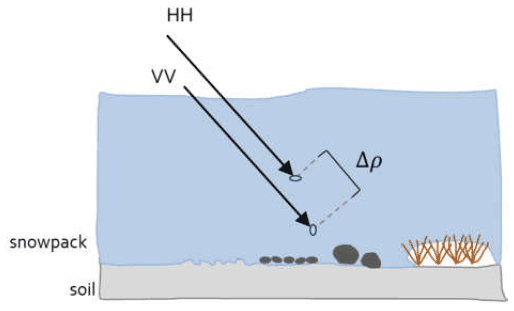
Figure 1Phase shift (Δρ) can also be caused by scattering effects within the snowpack or by surface roughness (including vegetation) (credit: Anna Wendleder).
2.3 Co-polar phase difference
CPD is a polarimetric method using the difference in the phase between HH and VV polarization channels. The phase difference refers to the difference in the propagation speed of a wavelength in a material as a function of polarization, which then causes a phase difference in the electromagnetic wave between polarizations. The phase of a single polarization is assumed to have a uniform distribution over [−π, π] (Leinss et al., 2014; Patil et al., 2020).
A relationship was found between CPD and snowfall by Chang et al. (1996) and Leinss et al. (2014) which induces a propagation delay among horizontal and vertical phases due to horizontal alignments of fresh snow crystals. Recent studies focused on the boreal region (Leinss et al., 2014, 2016) or were applied in arctic regions with no or sparse vegetation (Dedieu et al., 2018), so the application of the CPD method in the arctic remains poorly documented. It could be hypothesized that the CPD can describe the entire snowpack in such cold and dry environments. Strong vertical changes in density and grain size could also lead to a decrease in coherence so that the use of CPD information might not be suitable (i.e., when CCOH <0.5; see Fig. 1).
3.1 Study site
Qikiqtaruk/Herschel Island (69∘35′ N, 139∘06′ W) is located about 2 km off the Yukon Coast in the northwestern Canadian arctic (Fig. 2). With an approximate area of 108 km2, this island has a rolling topography (max. altitude: 183 m a.s.l.), dissected by numerous geomorphological forms such as gullies, valleys and polygonal soils (Short et al., 2011; Stettner et al., 2018). The permafrost on Qikiqtaruk/Herschel Island is continuous with a high ice content. Ground ice can be observed on the island in the form of ice wedges, ice lenses, or buried snowbanks, as observed by Pollard (1990). Results from Wolter et al. (2016) suggested that geomorphological processes, such as permafrost degradation, are strongly related to vegetation composition on Qikiqtaruk/Herschel. The active layer thickness varies from 45 to 90 cm in marine deposits (silty diamicton) and can reach over 110 cm in porous deposits (Lantuit and Pollard, 2008; Smith et al., 1989). A thickening of the active layer by 15 to 25 cm was documented on the island during the period from 1985 to 2005, as well as an increase in the mean annual air temperature by 2.7 ∘C between 1970 and 2005 (Burn and Zhang, 2009).
The spatial distribution of snow on the island is primarily based on topography due to the low tundra-type vegetation (Burn and Zhang, 2009). The snow is blown away from the uplands and accumulates in topographic depressions such as valleys and hummocky terrain (Burn and Zhang, 2009). The dominant wind direction is northwest with frequent storms in late August and September (Solomon, 2005). A study by Myers-Smith et al. (2011) indicates an increase in the canopy and vegetation height over the last century that can be expected to have an impact on the snow cover structure.
In this paper, we performed our measurements in the Ice Creek catchment (area of 1.54 km2) located at the eastern end of the island (Fig. 2). The digital elevation models (DEMs) from ArcticDEM (2 m resolution) indicate average slopes of 2.9∘ with maximums of 13.2∘ at altitudes ranging from 5 to 94 m (Porter et al., 2018).

Figure 2(a) Location of the study site in the arctic. (b) Visual extent of TerraSAR-X passages on Qikiqtaruk/Herschel Island. (c) Ice Creek study site including the location of measurements. The black crosses were revisited during each TerraSAR-X acquisitions (imagery provided by Worldview 01.01.1001, true color). The meteorological station belongs to Environment and Climate Change Canada (ECCC). AOI signifies area of interest.
3.2 Snow distribution over Ice Creek
3.2.1 Snow measurements
Two sampling strategies were used for the snowpit characterization (Table 1). First, detailed snowpit measurements were conducted along predefined locations at an average distance of 200 m between each site (Fig. 2c). The snowpit locations in the center of the Ice Creek catchment, as well as locations at the outlet of the catchment, were revisited during each TerraSAR-X (TSX; see Sect. 3.3) acquisition so that soil characteristics remain unchanged between snow sampling and satellite measurements. Snow depths were measured using a GPS snow depth probe around the snowpits, ensuring the representativeness of the snowpit location. This was conducted by measuring depths in a growing circle moving away from the snowpit location until an approximate diameter of 30 m was reached, which is typically the area required to ensure representativeness in tundra environments (Clark et al., 2011). Snowpits and SD measurements were then distributed spatially elsewhere in the catchment to refine the characterization of snow within the catchment. Additionally, two SD transects were conducted across the catchment to analyze the SD distribution in the study site. Both transects were established from the west side to the east side of the Ice Creek catchment. These transects were acquired on 1 May 2019 (Transect #2) and 4 May 2019 (Transect #1).
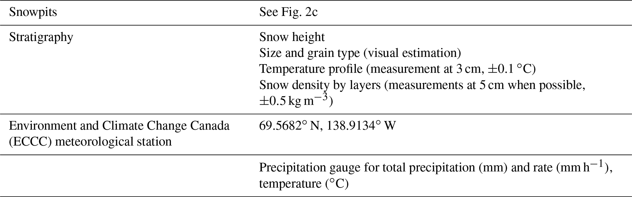
Detailed snow profiles were acquired in spring 2019 (mid-April to early May). In each site, we dug snowpits in a way to avoid direct solar illumination of the snow wall. High-resolution vertical profiles of density, temperature, grain size and type were conducted according to Fierz et al. (2009; see Table 1). Specifically, layered density profiles were obtained by extracting snow samples from each identified layer using a 100 cm3 density cutter and weighed using a Pesola light series scale. Temperature profiles were measured at 3 cm intervals using a Cooper digital thermometer, and profile measurements included shadowed surface temperature, as well as soil–snow interface.
From the above observations, each layer was classified according to their density and snow grain type across six classes following Fierz et al. (2009): (1) depth hoar, (2) wind slab, (3) surface hoar, (4) fresh snow, (5) melt–freeze crust and (6) ice layer. The snow depth and mean density of each layer classified were compiled for later linear regression analysis with TSX data from the same period. Regression analysis will be used to reach objective (2) of this paper.
3.2.2 Vegetation units
The classification of the different vegetation units was obtained from Eischeid (2015) following the initial definition developed by Smith et al. (1989). The classification was determined by the soil type, vegetation observed and geomorphological features. The dataset used in this study was derived from 2015 GeoEye satellite data (resolution: 1.65 m) (Eischeid, 2015). For the specific needs of this paper, we focused on the following specific classes: Arctic Willow and Dryas Vetch (hereinafter referred as Dryas), Arctic Willow and Lupine (Lupine), Shrub Zone (Shrub), and Willow Saxifrage Coltsfoot (Coltsfoot). These classes were selected given that they are physically and spatially different (see Fig. 3d), which is of primary importance from a snow microstructure and radar backscattering perspective.
The Lupine class is associated with an irregular and hummocky terrain (Eischeid, 2015, see Fig. 3d). The high variability in microtopography results in equally heterogeneous SD at a similar scale (Sturm and Holmgren, 1994). Erosion rates and moisture content will vary greatly following terrain instability (Eischeid, 2015). The Coltsfoot class is common in wetlands, where the ground is generally saturated and composed of shrubs (Eischeid, 2015). This vegetation class is located at the bottom of valleys, which is suitable for snow accumulation (Burn and Zhang, 2009). The Shrub class was added by Eischeid (2015) to the original classification by Smith et al. (1989) to reflect the growing importance of shrubs on the island. It is characterized by non-hydrophilic vegetation with lower soil moisture. Finally, the Dryas class is common on the gently undulating upland slopes (Smith et al., 1989). The associated soil type is a moderately well-drained Turbic Cryosol, which shows evidence of cryoturbation, as well as bare soil. Each snowpit characteristic and SD measurement were grouped by vegetation units to extract means and standard deviation by vegetation classes. The snowpits made along the two transects were grouped when they were at a distance less than 30 m, and statistics of distribution (average and standard deviation) were extracted to complete the data analysis.
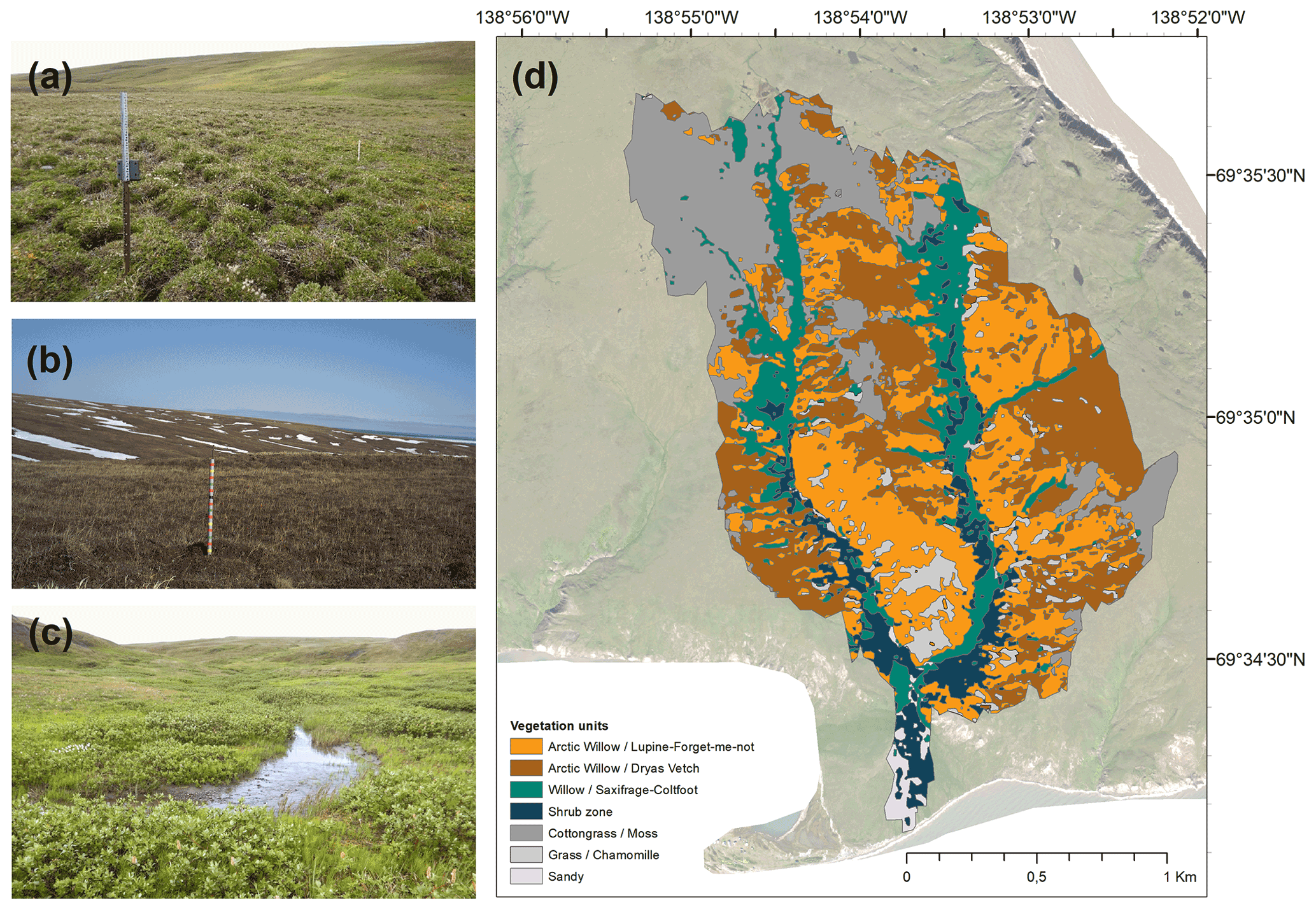
Figure 3Vegetation classes occurring in the Ice Creek catchment: (a) irregular and hummocky terrain observed in Lupine class (credit: Michael Fritz), (b) low vegetation in well-drained areas (such as Dryas) (photo by the authors), and (c) shrub and wetland (such as Coltsfoot class) (credit: Michael Fritz). (d) Vegetation unit's distribution in the study area (from Obu et al., 2017) as defined initially by Smith et al. (1989). The classes in grey are not included in the analysis.
3.3 Snow–SAR relationship
3.3.1 SAR acquisition and preprocessing
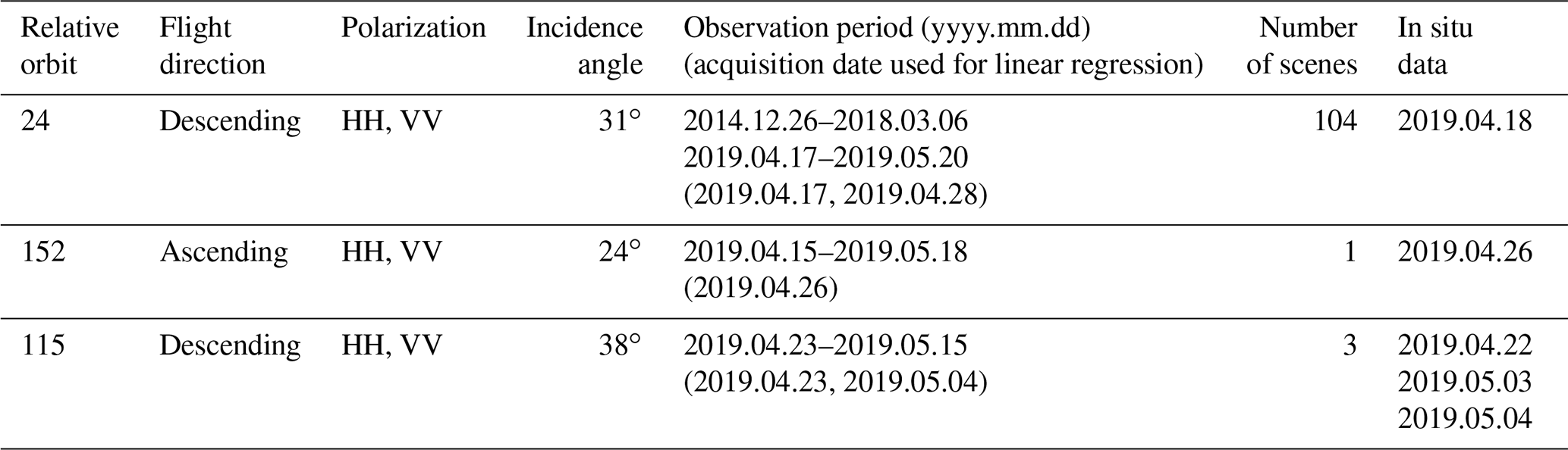
A total of five TSX acquisitions in HH and VV polarizations over three different orbits were obtained during spring 2019, encompassing areas where snow measurements and vegetation information was available (Table 2). Snowpits and SD measurements taken before and after (±2 d) each TSX acquisition were included in the analysis as no precipitation occurred and air temperature was stable during the field campaign. Additionally, a time series of TSX acquisitions for the 2015–2019 period (orbit 24, θ=31∘) was analyzed to evaluate the interannual variability in snow conditions on the island. The full TSX dataset was first processed at the DLR (German Aerospace Center). The preprocessing is described in Schmitt et al. (2015) and includes the determination of the Kennaugh elements, their radiometric calibration and orthorectification. The images were georeferenced in UTM (Universal Transverse Mercator) with a ground sampling distance of 5 m. To reduce speckle noise, we used the multi-scale multi-looking algorithm developed by Schmitt (2016) and Schmitt et al. (2015). CPD and CCOH can directly be derived from the radiometric and geometrically calibrated Kennaugh elements. The Kennaugh matrix describes the polarimetric information and allows us to differentiate the physical scattering mechanisms (e.g., double bounce, volume and surface scattering) affecting the signal, which in turn can be linked to snow characteristics. The following Kennaugh elements were used in the CPD equation:
where K7 is the phase shift between HH and VV phase center described as
and where K3 is the scattering difference between surface to double bounce:
To reduce the loss of coherence, a threshold was applied to CPD pixels in which CCOH was less than 0.5, following Leinss et al. (2014). Again, the Kennaugh elements were used in the CCOH equation.
Note that the notation of the Kennaugh matrix is labeled according to Schmitt et al. (2015). A total of 32 pixels had a CCOH less than 0.5, hence showing a random phase shift between waves which is not optimal for CPD applications. These pixels were therefore removed from the analysis. To discard the potential effect of slope on crystal grains orientation, 5 pixels with a slope greater than 10∘ were subsequently extracted (3 in the Dryas class, 2 in the Lupine class). To assess the temporal variability in the CPD signal, pixels were divided by vegetation class for the period 2015–2019.
Table 2TSX acquisition on Qikiqtaruk/Herschel Island. All orbits were used for linear regression with in situ snow measurements. Orbit 24 has a sufficient time series and was used to extract temporal evolution of CPD.
3.3.2 Linking snow depth to CPD
Implication of snow geometry
We focused on the SD variability between vegetation classes. We also evaluated depth hoar fraction (DHF) given that King et al. (2018) found that X-band backscattering is highly sensitive to depth hoar grains. DHF is the depth hoar ratio within the total depth of a snowpit. This allowed us to assess if any discrepancies in SD retrieval can be linked to large grain size. In addition, horizontal structures such as ice layers and melt–freeze crusts were identified for the same purpose of testing the SD retrieval capabilities in different stratigraphic contexts. Dedieu et al. (2018) showed that the attenuation of the SAR signal was caused by ice layers of 3 to 5 cm thickness, but lingering uncertainties remain with regards to the contribution of thinner ice lenses such as the ones found on Qikiqtaruk/Herschel Island.
Topographic wetness index
SD retrieval is challenging because it is impacted by snow surface properties. SD retrieval with CPD may be impacted by the dielectric properties of the snow surface, since the main backscatter signal is expected at the snow–ground interface. High moisture content at the soil surface would potentially improve the performance of SD retrieval given that the penetration of the signal into the soil would be limited by the high dielectric constant of the soil. The topographic wetness index (TWI) was chosen to analyze the variance between vegetation groups as a potential indicator of variability. Given the high sensitivity of microwaves to wetness, the high variability in TWI between each vegetation class will lead to different responses in backscattering through changes in the dielectric constant of the soil. The TWI was first developed by Beven and Kirkby (1979) within the runoff model TOPMODEL using the following equation:
where tan β is the local slope, and a is the upslope area per unit which is obtained with the upslope area (the cells contributing to the runoff to the cells of interest, A) and the contour length (L) following . The upslope area calculated is based on the D8 flow direction algorithm (O'Callaghan and Mark, 1984), and the TWI values were computed based on the ArcticDEM constructed from the DigitalGlobe Constellation (Porter et al., 2018; resolution: 2 m). Each TWI value derived from the catchment was combined to vegetation classes and CPD cells as described above.
Analysis
The Shapiro–Wilk test was used to test the normality of distributions for SD and TWI. Since TWI and SD distributions did not respect a normal distribution, the variance in TWI and SD between each group was tested with the non-parametric test Welch's ANOVA in conjunction with a post hoc Games–Howell test. Welch's ANOVA allows testing at first if the differences between the groups are statistically significant, while the post hoc Games–Howell test highlights the differences between specific groups. It may be possible that some groups show no statistically significant difference of the means. For instance, we could expect no difference of the means on the SD and TWI between the groups Coltsfoot and Shrub as both vegetation units are located in areas well suited for snow and water accumulation. We use the Games–Howell test as it does not assume equal variances and sample sizes (Games and Howell, 1976).
We evaluated the correlation between snow characteristics and CPD using a linear regression analysis. The median value was extracted when more than one snow measurement was found in the same TSX pixel (5 m). Thus, a total of 371 pixels were used in the analysis (average number of snow measurements per pixel: 1.7). The median SDs by pixels were grouped by vegetation classes and orbit. The Durbin–Watson test and the Breusch–Pagan test were used to assess autocorrelations and homoscedasticity of distribution data. Significance for all tests was calculated with α=0.05.
4.1 Snow distribution
4.1.1 Snow depth and depth hoar fraction along transects
Measurements of SD from Transect #1 (Fig. 4) varied between 20 and 250 cm where the peak was measured at the valley bottom. Further west, SD values decreased substantially on the slope with values between 20 and 50 cm. The highest DHFs along the transect were found on the west side of the transect and on the slopes with an average of 0.76, while an average of 0.39 was observed on the east side of the catchment. Along Transect #2 (Fig. 4), snow cover was also deeper at the bottom of the valley (from 120 up to 200 cm) and decreased significantly on slopes and higher elevation areas (30 to 50 cm).
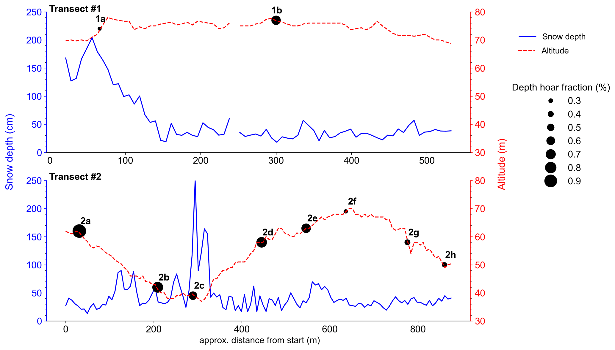
Figure 4Snow depth (SD) transects surveyed in the Ice Creek catchment. Transect #1 and Transect #2 show snow depth (solid line) and altitude (m.a.s.l., dashed line) along transect. Mean depth hoar fractions (DHFs) are indicated along transects by proportional size. Points 1a, 1b and 2c contain one observation. See Fig. 2c for their location in the catchment.
4.1.2 Snow characteristics by vegetation classes
Snow depth
The average SD within Ice Creek catchment was 47.4 cm ± 9.6 cm. The range of variability was substantial, with minimum value at 8.0 cm and a maximum at 212.0 cm. The standard deviation of the snow depth was variable yet strong among all classes (Table 3). The largest standard deviation measured was over Lupine (22.3 cm or 57 % of the mean SD) followed by Coltsfoot (67.6 cm or 54 % of the mean SD). Coltsfoot was by far characterized by a greater SD than any other class.
Despite the great deviation around the mean for each class, Welch's ANOVA (Table 4) shows that SD is significantly different between all vegetation groups (p value = 5−13). Games–Howell post hoc revealed that the Coltsfoot SD measurement is significantly different from the other classes, as well as Dryas. The difference between Lupine and Shrub is not significant.
Topographic wetness index
The average TWI was 6.1±1.6. The minimum and the maximum ranged between 2.5 and 14.7, while the average by vegetation classes ranged between 7.4 and 5.5 with a weak deviation around the means (Table 3). Coltsfoot showed the highest TWI which is consistent with its location in the valley (Fig. 3) and its vegetation group type, characterized by hydrophilic vegetation. Welch's ANOVA shows that the wetness index extracted with TWI is significantly different between all vegetation groups with a p value <0.001 (p value = 6−14), which again is expected to lead to different responses from TSX. The Games–Howell post hoc test revealed that the difference in TWI is not significant between Coltsfoot and Shrub units and between Dryas and Lupine (Table 5).
Depth hoar fraction
The DHF of the snowpack was larger than 0.5 for all vegetation classes. However, standard deviations of classes with shallow snow such as Lupine and Dryas were greater, whereas the standard deviation was lower than 0.1 for Coltsfoot for which the SD is the highest. At least one horizontal structure (ice layer or melt–freeze crust layer) was found in each snowpit. The average thickness of each ice or melt–freeze crust layer was 1.6 cm ± 0.7 cm, and the cumulative thickness average by snowpit was 4.5 cm ± 2.8 cm. The maximum ice thickness (4 cm) was found at the station downstream, which would suggest that the sensitivity of the CPD to ice layers should be generally lower than what was found by Dedieu et al. (2018). The high stratification otherwise may attenuate the signal.
Table 3Averaged SD and DHF for each of the vegetation classes.
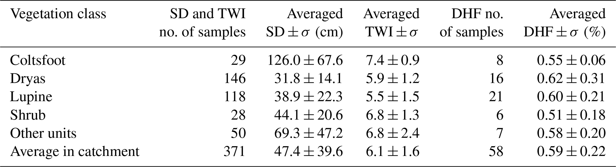
Table 4Post hoc analysis with Games–Howell for snow depth in vegetation classes (non-parametric test). Each row presents the variance between snow depth means from two different groups. All vegetation groups were tested on each other.
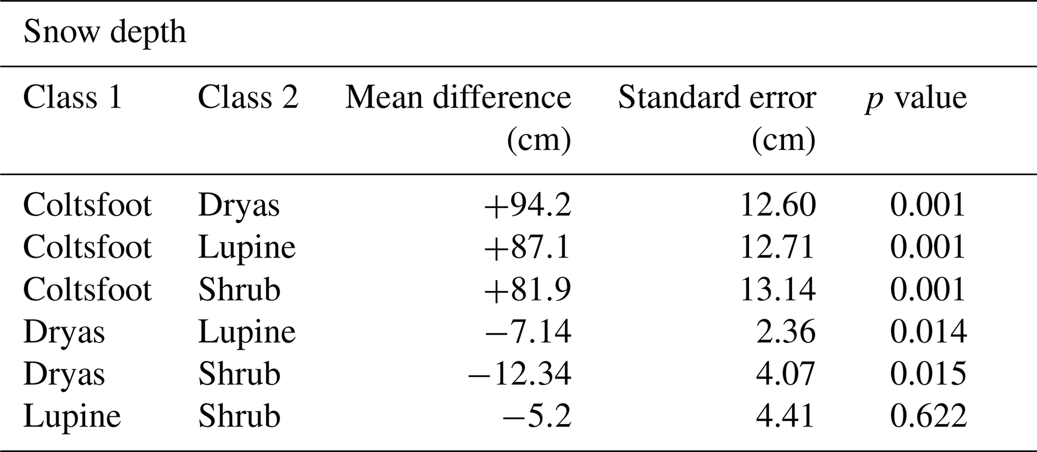
Table 5Post hoc analysis with Games–Howell for the TWI (non-parametric test). Each row presents the variance between TWI means from two different groups. All vegetation groups were tested on each other.

4.2 TerraSAR-X results
4.2.1 Spatial and temporal evolution of CPD
Figure 5a and b show the averaged temporal evolution of CPD and CCOH with descending orbit 24 (incidence angle = 31∘) for each vegetation class, as well as the confidence interval (95 %). The period with the presence of snow was set between mid-September and mid-May based on prior observations (Burn and Zhang, 2009; Stettner et al., 2018). Figure 5c shows the monthly average temperature and cumulative monthly precipitation on Qikiqtaruk/Herschel Island.
A periodicity was observed with the CPD signal with, on one side, the period of snow-free conditions in which the signal oscillates around zero and, on the other side, the period with snow in which the signal decreased over the season, suggesting an influence from the snowpack. For the 2014–2019 period, the mean CPD value during the snow was −8.59∘. The means of each winter are ranging between 13.41∘ (2014–2015) and −6.42∘ (2017–2018). During the snow-free condition, the average CPD over the same period increased to −0.87∘ (2014–2019). Maximum and minimum values during snow-free conditions ranged between −0.44∘ (2015) and −1.32∘ (2015–2016). The decrease generally started in January, when the average air temperature is at its coldest (−20 ∘C) except during the snow season of 2016–2017, when a warming occurred, increasing the average temperature by 5 ∘C for that year. The two classes with taller vegetation type (Coltsfoot and Shrub) stood out during the winters of 2014–2015 and 2016–2017. There the CPD decreased to −60∘ towards the end of the winter. The decrease in the CPD was therefore similar between the vegetation classes and is about −15∘.
Overall, the coherence stayed greater than the 0.5 threshold over the 2014–2019 period with an average of 0.71 ± 0.11. The signal was lower during the snow-free period when the average is 0.63 ± 0.11. The coherence then increased around 0.76 ± 0.08 during the winter. Coltsfoot and Shrub classes showed greater variation in the coherence over the seasons and the years compared to Lupine and Dryas classes. The average CCOH by vegetation classes ranged between 0.69 ± 0.07 (for Coltsfoot) and 0.72 ± 0.07 (for Dryas).
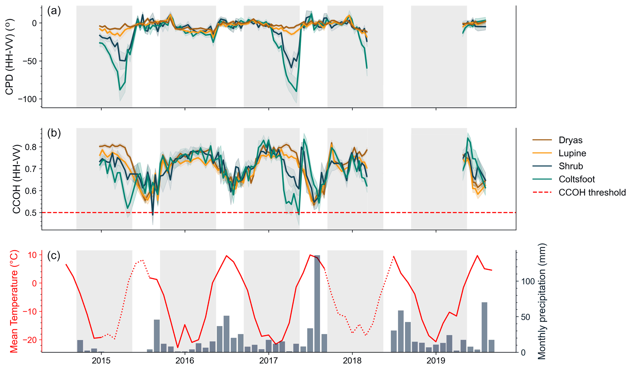
Figure 5(a) Average CPD and (b) average CCOH by vegetation class with interval of confidence (95 %) for orbit 24 (31∘, descending). Values were extracted from the GPS dataset (see Fig. 2c), in which NColtsfoot=33, NDryas=140, NLupine=118 and NShrub=29. The winter period (mid-September to mid-May) is shown in the shaded area. The window over which vegetation class information was extracted is the same size as a TSX pixel (5×5 m). (c) Meteorological data from Qikiqtaruk/Herschel Island station (dataset from Environment Canada, 2021). The meteorological station is not equipped with a telemetry system, and since the island is inaccessible during the winter, the lack of data during the winters of 2014–2015 and 2017–2018 was caused by a malfunction at the station. Air temperatures during these periods were gap-filled using Komakuk Beach meteorological station and are shown by the dotted red line. Please refer to Appendix A for further details on the method.
4.2.2 Retrieving SD per vegetation class using CPD
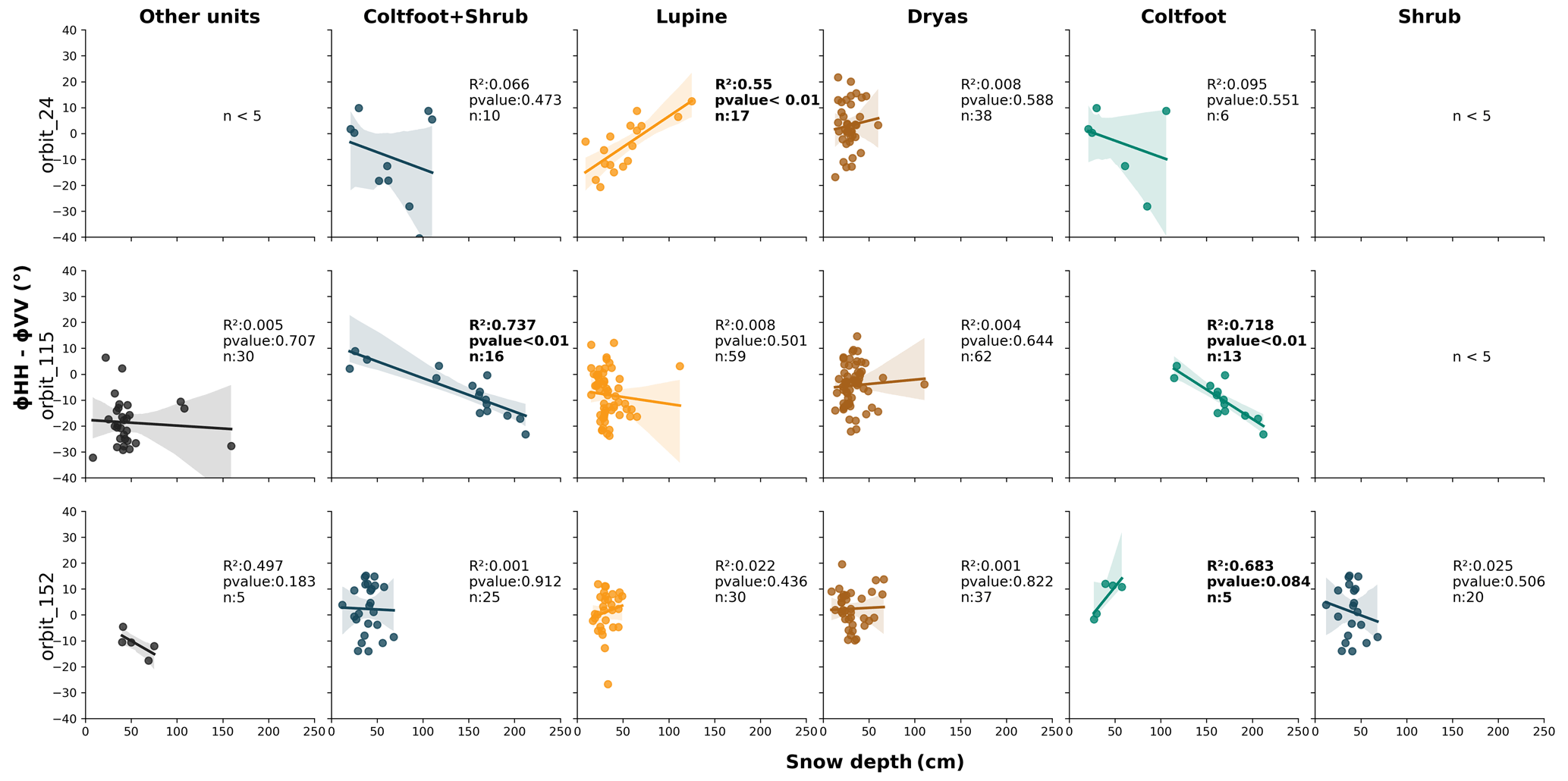
The dataset from 2019 was used to perform a simple linear regression analysis allowing us to assess whether there is a statistically significant relationship between snow measurements (layer depth of the depth hoar, wind slab, melt–freeze crust and ice layers and mean density of each layer) and CPD. No significant correlation was found other than SD, or the samples contained fewer than 10 observations, which resulted in elusive correlations (see Appendix A for more details). The best correlations between SD and CPD were found with Lupine (orbit 24, descending, incidence angle 31∘) and Coltsfoot (orbit 115, descending, incidence angle 38∘) (Table 6).
The Coltsfoot and Shrub classes were characterized by similar TWI mean values, as well as low TWI variance. These two classes were combined to be compared with other classes (named Coltsfoot + Shrub in Table 6). This grouping led to an improvement in the coefficient of determination of 0.044, as well as a decrease in p value and standard deviation. Samples with a coefficient of determination greater than 0.50 met the assumptions of homoscedasticity, as well as the absence of autocorrelation, except for the sample located in Coltsfoot + Shrub in orbit 115 and samples located in Coltsfoot in ascending orbit 152 (See Table B1 for further details). These results show clearly that CPD can be used to retrieve SD, albeit not in all vegetation classes.
Table 6R2, p value and standard deviation (R2±SD and p value ± SD in bold) results from linear regression analysis between SD and CPD obtained by vegetation classes and by orbits. The confidence interval was measured using the “bootstrap with replacement” resampling technique (Nbootstrap=1000). The standard deviation of R2 and the p value obtained by the technique are indicated in the results whose variance is explained to more than 50 %.
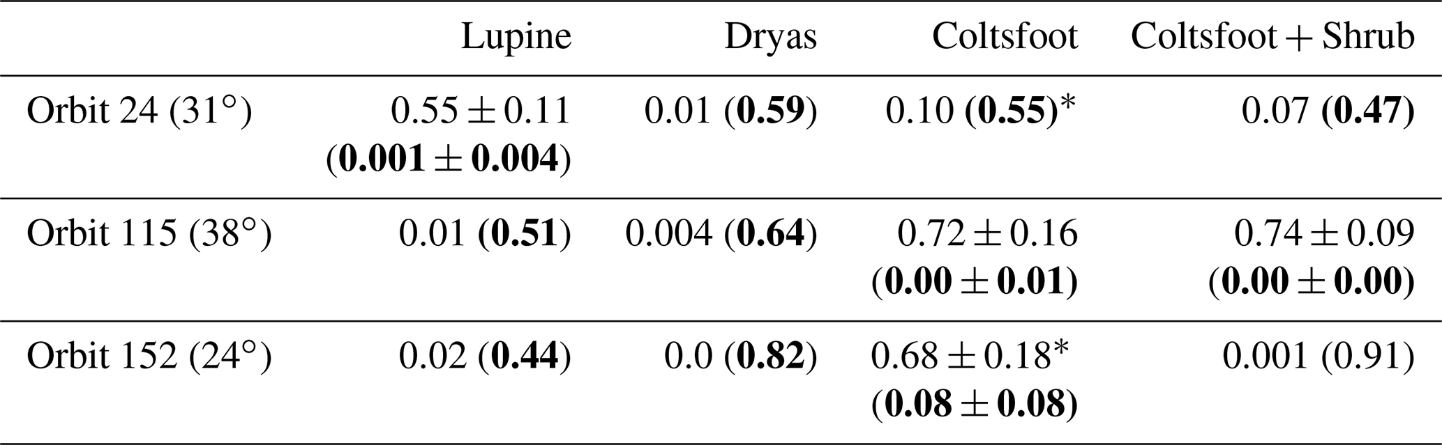
* Fewer than 10 observations.
5.1 Snow distribution on Qikiqtaruk/Herschel Island
5.1.1 Snow depth
On the study site, snow gets quickly redistributed across the landscape by winds. Burn and Zhang (2009) showed that SD distribution patterns were primarily driven by topography in close vicinity to the Ice Creeks. Our observations (Fig. 4) concur and expand on those from Burn and Zhang (2009) by highlighting the effect of microtopography and of vegetation in controlling SD. The SD was greater (>100 cm) in areas characterized by shrubs and wetlands (Coltsfoot), which are mainly associated with valley bottom locations. There is a significant difference in SD between Coltsfoot and any other class, which shows that snow gets blown away on high points and slopes and accumulates in spatially constrained areas at the valley bottom (Fig. 3d and c). By contrast, grass-type or shallow vegetation, such as Dryas and Lupine, is found in wind-exposed areas. Deeper snow was found over Lupine compared to Dryas. The microtopography may play a role in this difference, as the standard deviation of SD is greater in the Lupine class. There is greater variability in SD between the troughs and the top of hummocks, as documented by Wilcox et al. (2019). Thus, we can relate in this study that the distribution of snow in the Ice Creek catchment is driven primarily by vegetation and topography.
5.1.2 Depth hoar fraction
We suggest that the DHF is strongly driven by microtopography. During winter 2019, the DHF amounted to an average of 59 % of the snowpack (n=58). There is a greater standard deviation in these measurements in vegetation classes for which the average SD is lower (less than 40 cm average depth) such as Lupine and Dryas. The effect of microtopography allows snow capture in hummock hollows early in the season, and the thermal gradient from the ground to the surface varies accordingly (King et al., 2018; Wilcox et al., 2019). Depth hoar develops when a strong thermal gradient occurs between the ground and the snow surface. There are two situations when a strong gradient occurs: (1) when the SD is low and (2) when the soil is warm and the snow surface is cold. Sturm and Holmgren (1994) have shown that the depressions in tussocks or hummock are warmer than the top. The thermal gradient found in this type of vegetation class may therefore explain the large standard deviation of DHF found in Lupine class. Thus, the soil wetness should be higher in the hollows, but that effect might not be captured by the TWI used in this paper as its spatial resolution relies on a 2 m resolution DEM.
5.2 CPD spatiotemporal evolution and SD correlation
The high-resolution vegetation classification used in this paper allowed us to show that CPD varies greatly according to seasons and vegetation class (Fig. 5). Overall, the CPD signal decreased during winter and increased rapidly during melt. This concurs with observations from Leinss et al. (2014, 2016) made in Sodankylä, Finland. According to the model developed by Leinss (2014, 2016), the strong CPD decrease observed in the 2015 and 2017 winters over shrub areas could be explained by fresh snow accumulation or dominance of horizontal structures. However, the snow distribution analysis showed that the Shrub class has shallow snow, making it, SD-wise, significantly different from the Coltsfoot class, meaning the result does not show that the measured CPD signal is entirely governed by the snowpack. The CPD evolution over different vegetation classes is significantly different between two distinct groups: tall vegetation zones (Coltsfoot and Shrub) and low vegetation zones (Lupine and Dryas). The small decrease observed for Lupine and Dryas classes during the snow season (Fig. 5) could indicate an influence from the ground as the snow depth measured is less than 30 cm and highly stratified. However, the effect from inhomogeneities within the snowpack does not support this case as the CCOH is greater than 0.5 for each pixel. Dryas is characterized by the lowest TWI, which could lead to less backscattering at the snow–ground interface and hence decrease the change in the snow season. High DHF in Lupine vegetation class indicates a potential of higher TWI in the tussock's hollow, which might not be captured by the TWI. Hence, the TWI variability within a TSX pixel at this vegetation class area could also explain the low decrease in CPD observed in Fig. 5.
Although the snowpack was highly stratified, each ice layer or melt–freeze crust was on average less than 2 cm thick, which is thinner than the ice layers in the snowpacks studied by Dedieu et al. (2018). It may explain why the linear regression analysis of CPD shows the best results with the total SD (i.e., less sensitive to small crusts), which has never been observed before.
A high level of moisture in the ground will lead to major dielectric contrast at the snow–soil interface, hence limiting the penetration depth of the radar signal (Duguay et al., 2015). Thus, the sensitivity of the signal to ground conditions decreases. Duguay et al. (2015) also showed a strong saturation of TSX signal in the areas with shrubs greater than 50 cm. Warmer ground temperatures were previously observed in permafrost (e.g., Myers-Smith and Hik, 2013; Domine et al., 2016), which could delay the freezing process and enhance the contrast at the snow–ground interface. In the case of the study area, Myers-Smith et al. (2019) report an increase in the canopy where the measured shrubs at the bottom of the valley were more than a meter.
The TWI variance analysis shows that there is no significant variance between Coltsfoot and Shrub classes and between Lupine and Dryas classes, which could explain the strong decrease in the signal observed in mid-winter (Fig. 5). A high TWI indicates a high water accumulation potential and hence a higher saturation of the soil. In the microwave range, soil saturation increases the dielectric properties of the soil. The sensitivity of the X-band radar signal is then higher, which allows the interface between the snowpack and the ground to be well discriminated. Thus, CPD captures snow accumulation well across winter in areas with a higher potential of soil moisture, while soils with a lower potential of moisture are likely to contribute to the CPD signal and thus reduce the correlation between snow depth and CPD signal.
We suggest the increase in the R2 depends on the soil moisture because there is less contribution from the ground to the backscatter signal. A higher incidence angle (>30∘) improves the results, agreeing with Leinss et al. (2014). The use of the TWI is promising for the snow-SAR dynamics as it is easy to compute and relies on topographic datasets that are now widely available for the entire arctic. Furthermore, no correlation was found between retrieval performance of SD and DHF, suggesting that the poor performance over the Dryas class is explained by soil contributions. The relatively conclusive results for the Lupine class at orbit 24 show an inverse correlation (Fig. 6) which contradicts Leinss et al. (2014). We hypothesize that the tussock depressions are preferential areas for the formation of depth hoar, caused by the effect of microtopography. Thus, vertical structures are dominant in the snowpack, which could explain an increase in vertical structure in which the snowpack is deeper in this vegetation class. Further analysis should be done on the soil moisture and on the effect of the depth hoar distribution to better capture the wetness of hummocky areas and how it can improve retrievals of SD.
This study was the first to investigate the potential of co-polar phase difference (CPD) derived from TerraSAR-X data in combination with snowpit characterization over Qikiqtaruk/Herschel Island. We were able to find a variability in SD and TWI depending on vegetation classes extracted from a high-resolution map of vegetation cover. Classifying snowpits by vegetation classes on Qikiqtaruk/Herschel Island shows respectable results, helping to demonstrate the effect of topography and hence the moisture rate of the ground on the CPD signal. The 2019 dataset shows a high heterogenous snowpack with different ice layers and with a DHF representing on average more than half of the snowpack.
Despite this complex snowpack, we demonstrate a correlation between the CPD and the SD when certain conditions are met. With a high incidence angle (>30∘) and a high TWI (>7.0), a significant correlation between SD and CPD can be found with an R2 of 0.72. CPD cannot be used to extract the fresh snow in an arctic context as the penetration of the electromagnetic wave tends to go through the entire snowpack.
The in situ data used for the present study do not cover the entire winter on Qikiqtaruk/Herschel Island, which brings uncertainties on snow depth characterization with CPD. The lack of consistent stratigraphy measurement over the winter is still a major limit in snow studies. Consistent stratigraphy measurement over the winter would improve the understanding of the snowpack metamorphism regime.
The maritime climate of Qikiqtaruk/Herschel Island may advance the snowmelt period and provoke a shift to a wet metamorphism regime in the snowpack. To address the remaining question about the specific climate of the study site, we compared our statistics to the classification proposed by Royer et al. (2021) and observed a good fit with the herbaceous and low shrub tundra snow class (Table B2). The snow characteristics observed over the Ice Creek catchment are consistent with the literature.
The standard deviations of the mean snow depth from our study site and from the Royer et al. (2021) classification are both greater than 80 %. The local topography inherited from the last glaciation (Late Wisconsin) is specific to Qikiqtaruk/Herschel Island and could explain higher snow depth and therefore higher SWE (snow water equivalent) and density. The maritime effect observed on Qikiqtaruk (Cray and Pollard, 2015) could also explain the warmer mean temperature during winter. All study sites used in the Royer et al. (2021) classification are in the east of Canada. Further studies and datasets from the western part of Canada would greatly improve the snow classification.
A focus of future studies could be the threshold sensitivity to TWI and the incidence angle of snow depth retrievals to map snow depth in such environments and to evaluate the potential of using interpolation tools to cover the gaps in SD information over vegetation types. SD variability within a TSX pixel should be studied further, especially in hummocky areas where the highest variability was found, which could suggest a variability in the TWI as well. Statistical approaches using the coefficient of variation of snow depths (CVsd), as suggested by Winstral and Marks (2014) and Liston (2004), could be an interesting avenue in the development of a representative mapping of the terrain. Meloche et al. (2022) demonstrated recently the effectiveness of CVsd to improve passive microwave SWE retrievals in a similar environment to that found on Herschel Island (i.e., arctic snowpack with tundra vegetation type).
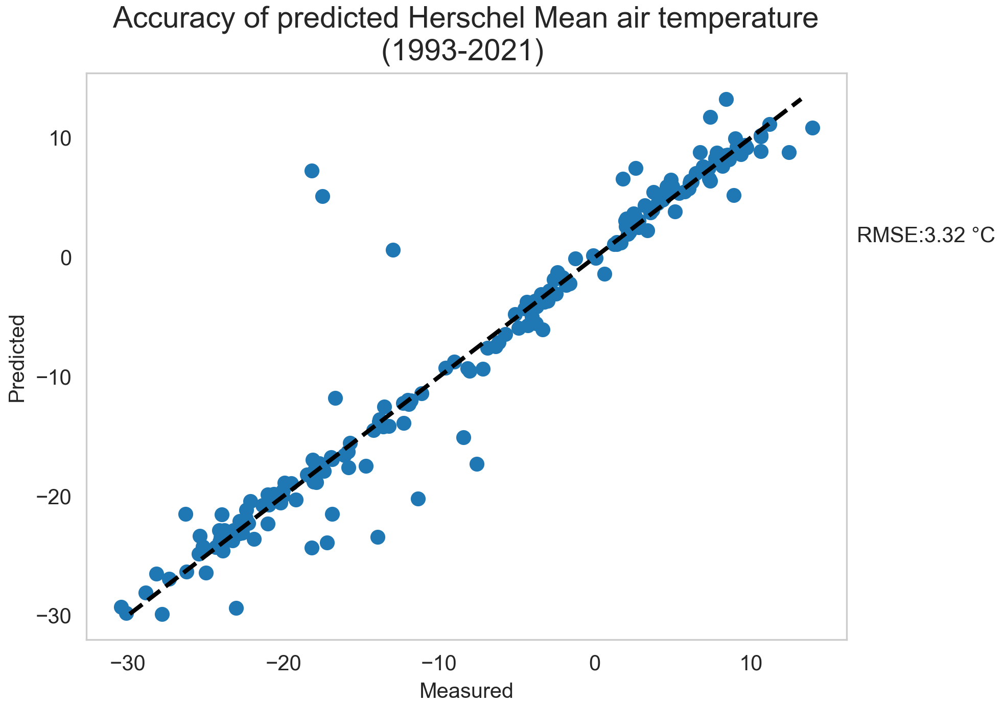
Figure A1Result from linear regression between air temperature measured on Herschel Island and predicted value using the Burn and Zhang (2009) equation.
The meteorological station is not equipped with a telemetry system, and since the island is inaccessible during the winter, the lack of data during the winters of 2014–2015 and 2017–2018 was caused by a malfunction at the station. Air temperatures during these periods were gap-filled using Komakuk Beach meteorological station as performed by Burn and Zhang (2009). The following equation was applied on the Komakuk Beach dataset:
where Th is the monthly mean air temperature at Herschel Island and Tk at Komakuk Beach. Predicted values showed good correlation (R2: 0.93; p value = <0.001) with RMSE of 3.32 ∘C (Fig. A1).
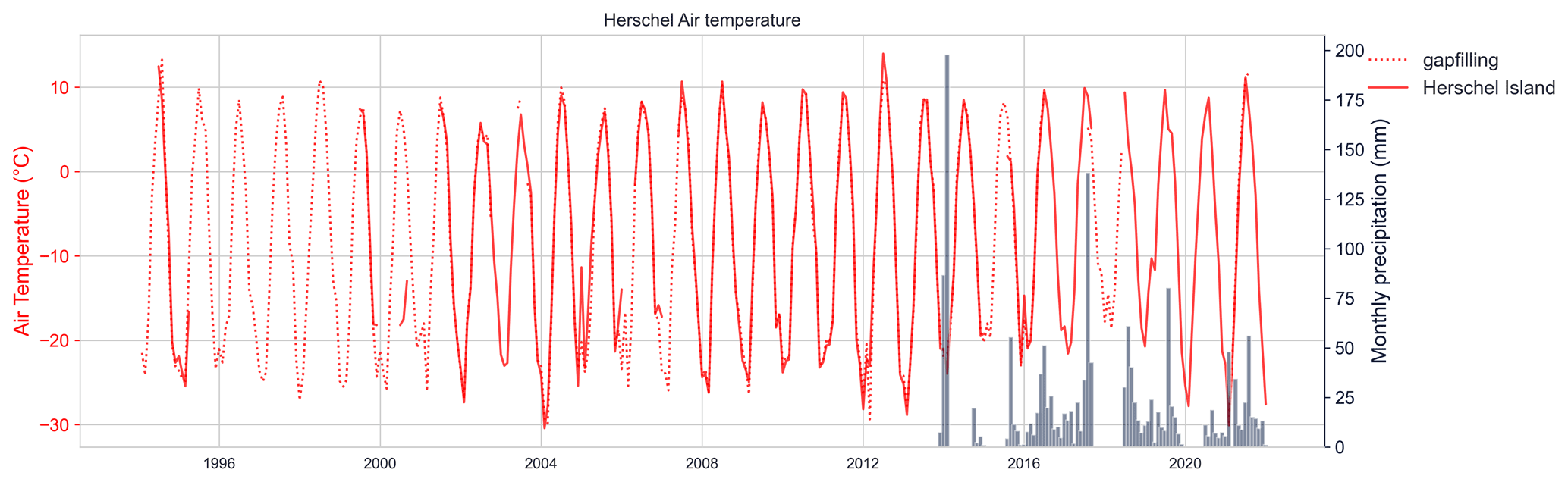
Figure A2Comparison during 1994–2022 of air temperature measured on Herschel Island and predicted value using the Burn and Zhang (2009) equation.
Figure A2 shows a visual comparison between the air temperature predicted and measured along the time series. Unfortunately, no precipitation datasets were available at Komakuk Beach station.
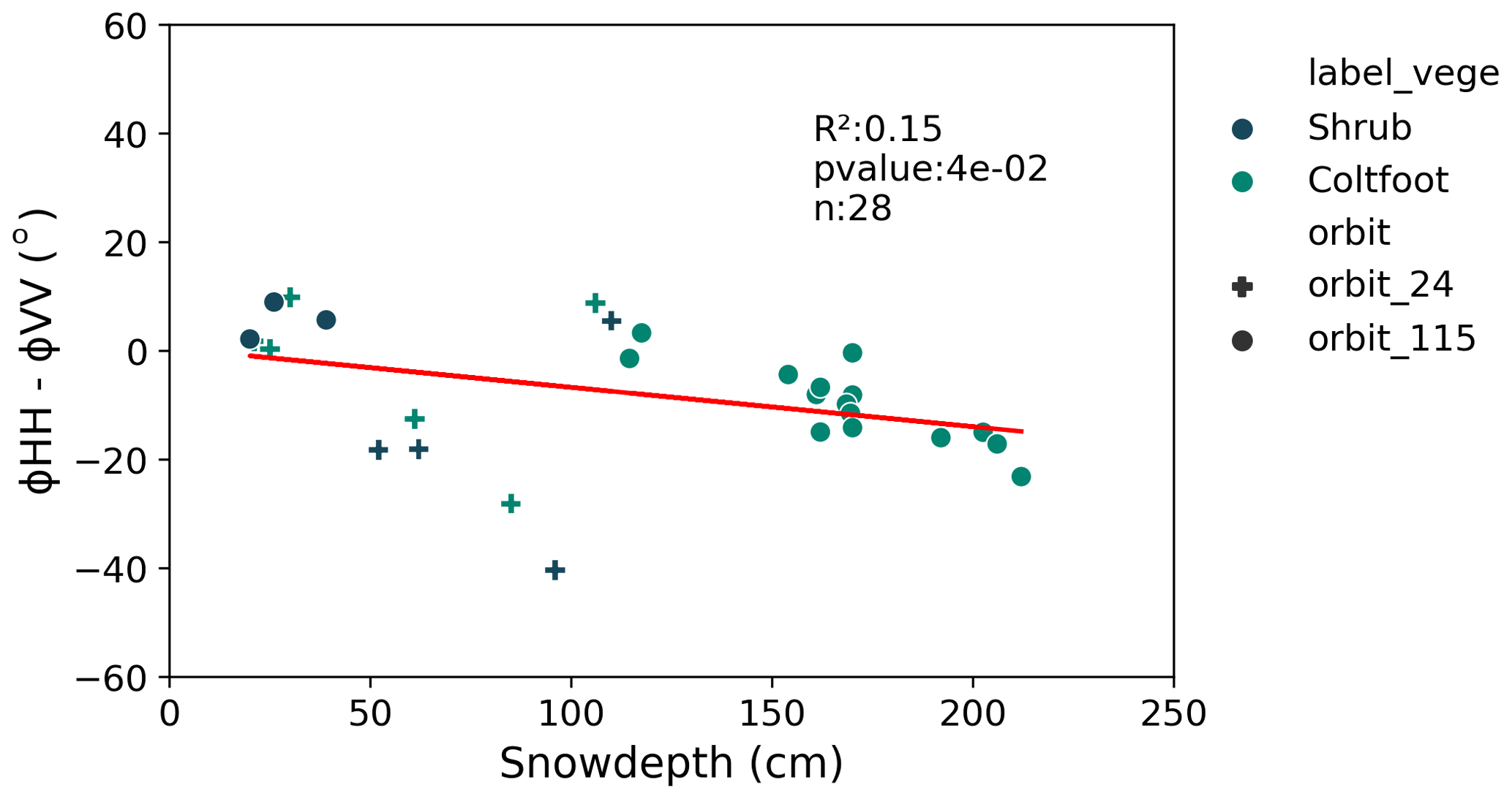
Figure B1Linear regression between CPD and snow depth on descending orbit (orbits 24 and 115) without TWI threshold.
Table B1Complementary results retrieved during the linear regression analysis. The standard deviation with bootstrap is not show as the results with R2 greater than 0.5 have samples with fewer than eight observations.
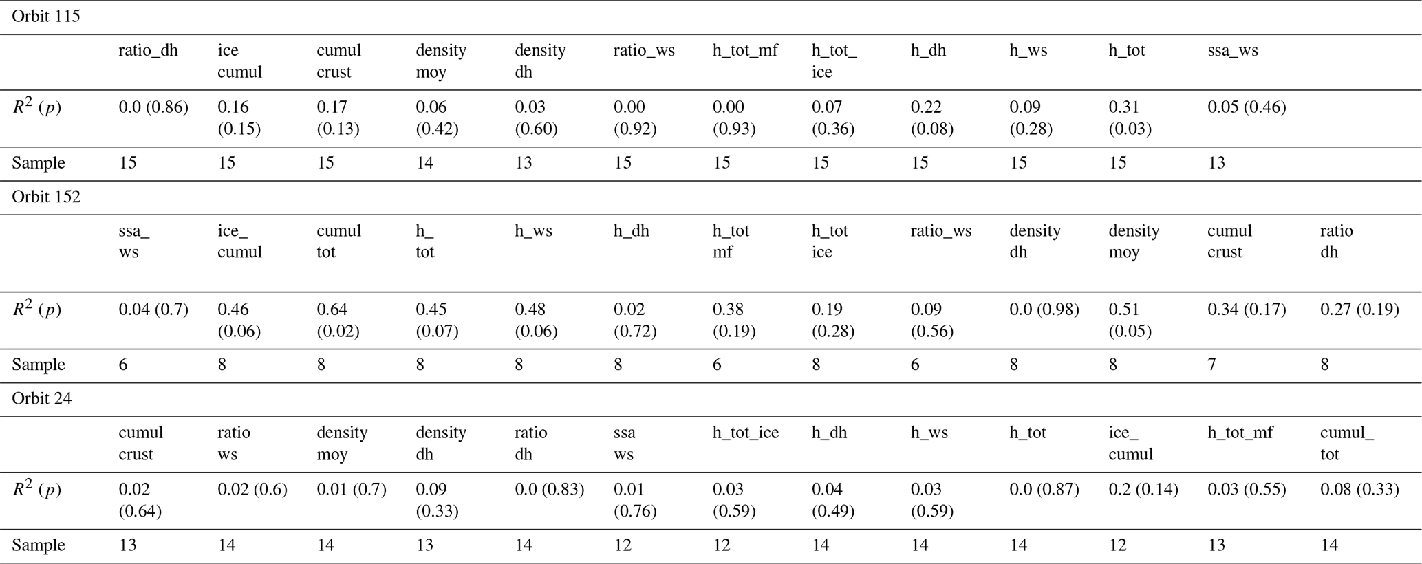
Table B2Comparison of snow characteristics with the Royer et al. (2021) classification. Mean temperature was extracted from the 1974–2019 meteorological station from Qikiqtaruk/Herschel Island and for the winter season (December to March as defined by Royer et al., 2021).
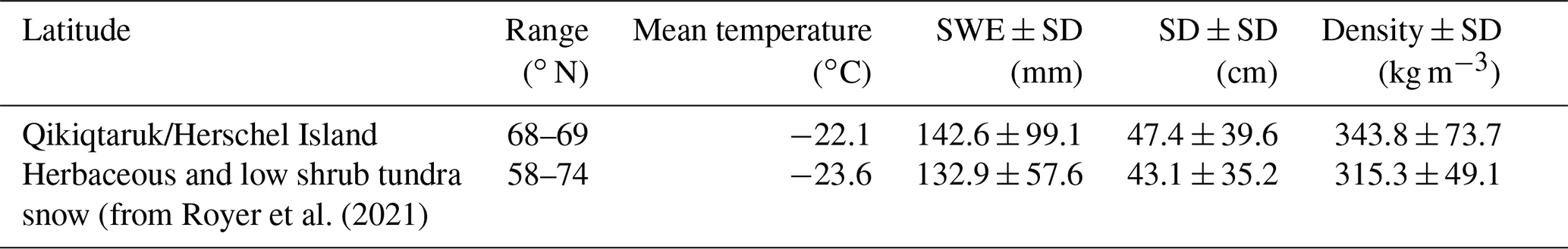
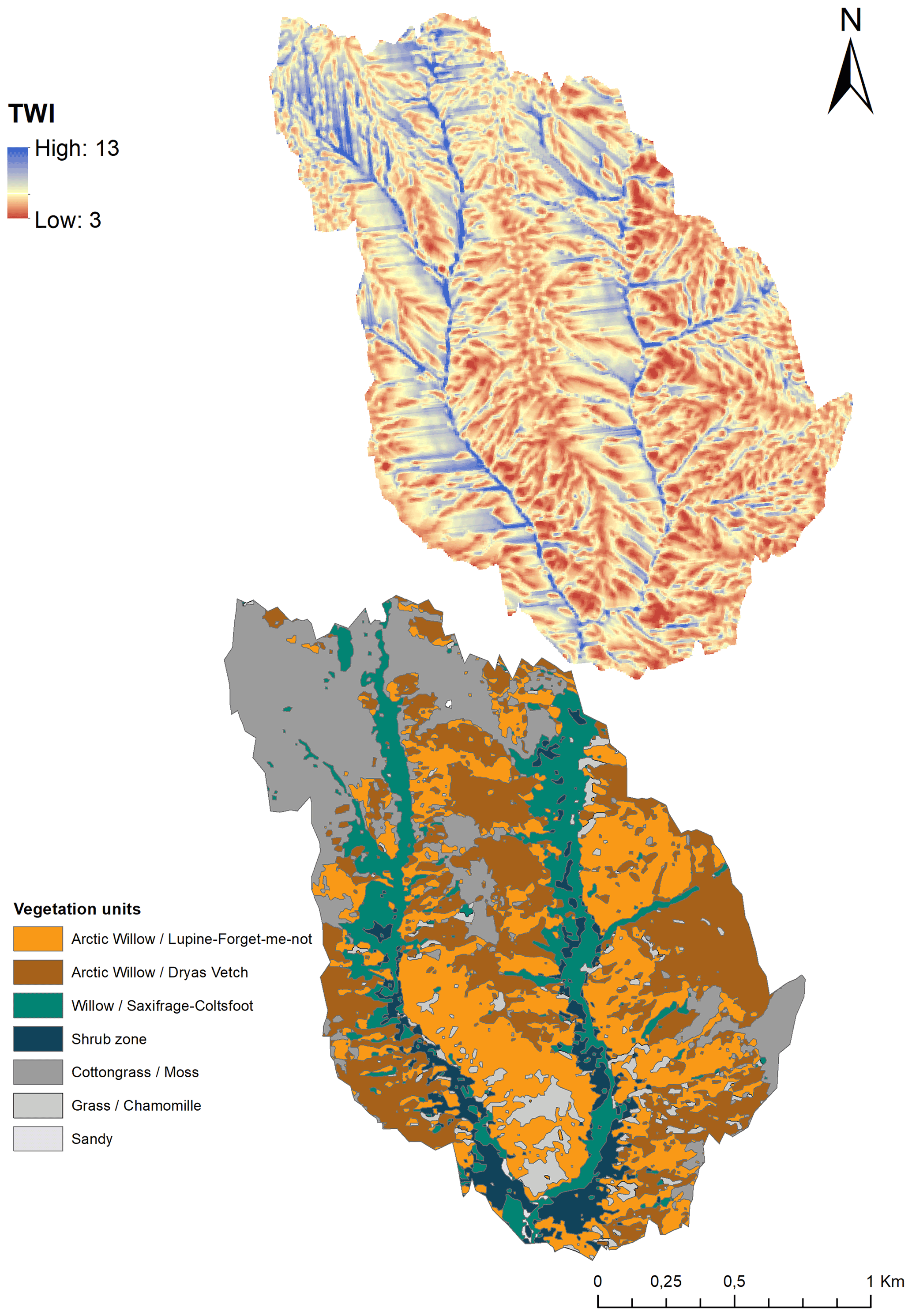
Figure B2Topographic wetness index (TWI) map compared to vegetation units located on Qikiqtaruk/Herschel Island.
Table B1 shows the complementary results retrieved during the linear regression analysis between CPD and every snow variable measured on the field. Results with R2 greater than or equal to 0.5 are shown in bold. The samples may vary when a measurement was not possible during the field campaign.
Each variable describes a characteristic sampled in the snowpit.
-
H_tot: snow depth (cm)
-
H_ws: wind slab height (cm)
-
H_dh: depth hoar height (cm)
-
H_tot_ice: snow height to the first ice layer observed in the snowpit (cm) and ice layer thickness greater than 2 cm
-
H_tot_mf: snow height to the first melt–freeze crust (cm)
-
Density_moy: average snow density (kg m−3)
-
Density_dh: average density for the depth hoar layer (kg m−3)
-
Ssa_ws: average snow surface area measured in the wind slab layer
-
Ratio_df: depth hoar fraction in the snowpit (%)
-
Cumul_tot: cumulative thickness of horizontal layers (melt–freeze crust, ice lens, in cm)
-
Ice_cumul: cumulative thickness of ice lens (cm)
-
Cumul_crust: cumulative thickness of melt–freeze crust (cm)
-
Ratio_ws: wind slab ratio in the snowpit (%).
C1 Homoscedasticity
Linear least squares regression assumes that the residuals come from a population in which the variance is constant. When heteroscedasticity is present, the result is therefore unreliable. The Breusch–Pagan statistical test evaluates the assumption of homoscedasticity, i.e., the consistency of the error variance in a linear regression model.
Table C1Statistical test results for CPD and snow depth correlation analysis. Each model represents a divided sample in function of vegetation class and TSX orbit. Results with an R2 greater than 0.5 are shown. The Durbin–Watson test (DW) and the Breusch–Pagan test (LMS, Lagrange multiplier statistic) were selected to assess the autocorrelation for the first and the homoscedasticity for the latter.
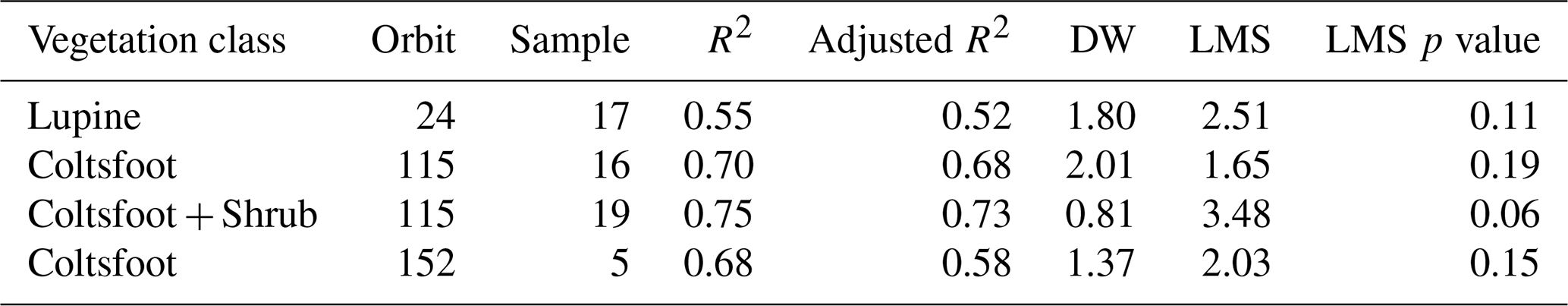
The assumptions are as follows.
-
Null hypothesis (H0). Homoscedasticity is present.
-
Alternative hypothesis (Ha). Homoscedasticity is not present (heteroscedasticity is present).
If the p value of the Lagrange multiplier statistic (LMS) is greater than 0.05, the probability of homoscedasticity is greater than 5 %. The null hypothesis is therefore retained. In the opposite case (p value < 0.05), the probability of homoscedasticity is less than 5 %. The alternative hypothesis is then adopted.
C2 Autocorrelation
The Durbin–Watson test (DW) is used to test the autocorrelation of residuals in linear regression models. It assesses whether the residuals are independent.
The assumptions are as follows.
-
H0. There is no correlation between the residuals.
-
Ha. The residuals are autocorrelated.
The results are expected between 0 and 4. Values between 1.5 and 2.5 indicate no autocorrelation. Results near 0 show positive autocorrelation, while results near 4 show negative autocorrelation.
Data and code are made available upon request to the corresponding author.
JVS performed this study as part of her master thesis project, co-supervised by AL and HL. JVS, SS, AL, AW and HL designed the methodology. JVS wrote the code and performed the field measurements and the analysis. The original idea and method were developed by JVS, AL and HL. AW and AS performed the SAR preprocessing, AlR, AcR, AW, AL, AS and JPD supported the SAR analysis. The manuscript was written by JVS and edited by all the co-authors.
The contact author has declared that neither they nor their co-authors have any competing interests.
Publisher's note: Copernicus Publications remains neutral with regard to jurisdictional claims in published maps and institutional affiliations.
The authors acknowledge the use of the ArcticDEM (© 2019 Polar Geospatial Center) and the TerraSAR-X data (© DLR 2019). We would like to thank the Aurora Research Institute, the Yukon Territorial Government and Yukon Parks (Herschel Island Qikiqtaruk Territorial Park) for administrational and logistical support, as well as the Inuvialuit people for the opportunity to conduct research on their traditional lands. Joëlle Voglimacci-Stephanopoli would like to thank Vincent Sasseville for the fieldwork support and Silvan Leinss for the many exchanges and discussions on the CPD method. The authors would like to thank Georg Fisher, the reviewers and the editor, Carrie Vuyovich, for their help in improving this paper.
This research has been supported by the Horizon 2020 (grant no. Nunataryuk (773421)), Mitacs Globalink and Polar Knowledge Canada.
This paper was edited by Carrie Vuyovich and reviewed by two anonymous referees.
AMAP: Snow, Water, Ice and Permafrost in the Arctic (SWIPA) 2017, ISBN 978-82-7971-101-8, https://www.amap.no/documents/doc/snow-water-ice-and-permafrost-in-the-arctic-swipa-2017/1610 (last access: 27 May 2022), 2017.
Berteaux, D., Gauthier, G., Domine, F., Ims, R. A., Lamoureux, S. F., Lévesque, E., and Yoccoz, N.: Effects of changing permafrost and snow conditions on tundra wildlife: critical places and times, Arct. Sci., 3, 65–90, https://doi.org/10.1139/as-2016-0023, 2017.
Beven, K. J. and Kirkby, M. J.: A physically based, variable contributing area model of basin hydrology, Hydrol. Sci. Bull., 24, 43–69, https://doi.org/10.1080/02626667909491834, 1979.
Bokhorst, S., Pedersen, S. H., Brucker, L., Anisimov, O., Bjerke, J. W., Brown, R. D., Ehrich, D., Essery, R. L. H., Heilig, A., Ingvander, S., Johansson, C., Johansson, M., Jónsdóttir, I. S., Inga, N., Luojus, K., Macelloni, G., Mariash, H., McLennan, D., Rosqvist, G. N., Sato, A., Savela, H., Schneebeli, M., Sokolov, A., Sokratov, S. A., Terzago, S., Vikhamar-Schuler, D., Williamson, S., Qiu, Y., and Callaghan, T. V: Changing Arctic snow cover: A review of recent developments and assessment of future needs for observations, modelling, and impacts, Ambio, 45, 516–537, https://doi.org/10.1007/s13280-016-0770-0, 2016.
Burn, C. R. and Zhang, Y.: Permafrost and climate change at Herschel Island (Qikiqtaruq), Yukon Territory, Canada, J. Geophys. Res.-Earth, 114, 1–16, https://doi.org/10.1029/2008JF001087, 2009.
Calonne, N., Flin, F., Geindreau, C., Lesaffre, B., and Rolland du Roscoat, S.: Study of a temperature gradient metamorphism of snow from 3-D images: time evolution of microstructures, physical properties and their associated anisotropy, The Cryosphere, 8, 2255–2274, https://doi.org/10.5194/tc-8-2255-2014, 2014.
Chang, P. S., Mead, J. B., Knapp, E. J., Sadowy, G. A., Davis, R. E. and Mcintosh, R. E.: Polarimetric Backscatter from fresh and metamorphic snowcover at millimeter wavelengths, IEEE T. Antenn. Propag., 44, 58–73, https://doi.org/10.1109/8.477529, 1996.
Clark, M. P., Hendrikx, J., Slater, A. G., Kavetski, D., Anderson, B., Cullen, N. J., Kerr, T., Örn Hreinsson, E., and Woods, R. A.: Representing spatial variability of snow water equivalent in hydrologic and land-surface models: A review, Water Resour. Res., 47, W07539, https://doi.org/10.1029/2011WR010745, 2011.
Colbeck, S. C.: Theory of metamorphism of wet snow, United States Army Corps of Engineers, Hanover, NH, USACRREL Report 73, 1–11, 1973.
Colbeck, S. C.: An overview of seasonal snow metamorphism, Rev. Geophys., 20, 45–61, https://doi.org/10.1029/RG020i001p00045, 1982.
Cray, H. A. and Pollard, W. H.: Vegetation recovery patterns following permafrost disturbance in a Low Arctic setting: Case study of Herschel Island, Yukon, Canada, Arctic, Antarct. Alp. Res., 47, 99–113, https://doi.org/10.1657/AAAR0013-076, 2015.
Dedieu, J., Negrello, C., Jacobi, H., Duguay, Y., Boike, J., Bernard, E., Westermann, S., Gallet, J., and Wendleder, A.: Improvement of snow physical parameters retrieval using SAR data in the Arctic (Svalbard), in International Snow Science Workshop, Innsbruck, Austria, 303–307, https://hal.archives-ouvertes.fr/hal-01963077/file/Bernard_20ISSW2018.pdf (last access: 27 May 2022), 2018.
Dolant, C., Montpetit, B., Langlois, A., Brucker, L., Zolina, O., Johnson, C. A., Royer, A., and Smith, P.: Assessment of the Barren Ground Caribou Die-off During Winter 2015–2016 Using Passive Microwave Observations, Geophys. Res. Lett., 45, 4908–4916, https://doi.org/10.1029/2017GL076752, 2018.
Domine, F., Barrere, M., and Morin, S.: The growth of shrubs on high Arctic tundra at Bylot Island: impact on snow physical properties and permafrost thermal regime, Biogeosciences, 13, 6471–6486, https://doi.org/10.5194/bg-13-6471-2016, 2016.
Domine, F., Picard, G., Morin, S., and Barrere, M.: Major Issues in Simulating some Arctic Snowpack Properties Using Current Detailed Snow Physics Models, Consequences for the Thermal Regime and Water Budget of Permafrost, J. Adv. Model. Earth Sys., 11, 34–44, https://doi.org/10.1029/2018MS001445, 2018a.
Domine, F., Belke-Brea, M., Sarrazin, D., Arnaud, L., Barrere, M., and Poirier, M.: Soil moisture, wind speed and depth hoar formation in the Arctic snowpack, J. Glaciol., 64, 990–1002, https://doi.org/10.1017/jog.2018.89, 2018b.
Duguay, Y., Bernier, M., Lévesque, E., and Tremblay, B.: Potential of C and X band SAR for shrub growth monitoring in sub-arctic environments, Remote Sens., 7, 9410–9430, https://doi.org/10.3390/rs70709410, 2015.
Eischeid, I.: Mapping of soil organic carbon and nitrogen in two small adjacent Arctic watersheds on Herschel Island, Yukon Territory, University of Hohenheim, https://doi.org/10.013/epic.47347.d001, 2015.
Fierz, C., Armstrong, R., Durand, Y., Etchevers, P., Greene, E., McClung, D., Nishimura, K., Satyawali, P., and Sokratov, S.: The International Classification for Seasonal Snow on the Ground (ICSSG), Tech. Rep., IHP-VII Technical Documents in Hydrology, No. 83, IACS Contribution No. 1, UNESCO-IHP, https://unesdoc.unesco.org/ark:/48223/pf0000186462 (last access: 27 May 2022), 2009.
Frei, A., Tedesco, M., Lee, S., Foster, J., Hall, D. K., Kelly, R., and Robinson, D. A.: A review of global satellite-derived snow products, Adv. Sp. Res., 50, 1007–1029, https://doi.org/10.1016/j.asr.2011.12.021, 2012.
Games, P. A. and Howell, J. F.: Statistics Key words: Multiple Comparisons; iances; Unequal Sample Sizes Means; Heterogeneous Games and Howell, J. Educ. Stat., 1, 113–125, 1976.
Goodrich, L. E.: The influence of snow cover on the ground thermal regime, Can. Geotech. J., 19, 421–432, https://doi.org/10.1139/t82-047, 1982.
Gouttevin, I., Menegoz, M., Dominé, F., Krinner, G., Koven, C., Ciais, P., Tarnocai, C., and Boike, J.: How the insulating properties of snow affect soil carbon distribution in the continental pan-Arctic area, J. Geophys. Res.-Biogeo., 117, 1–11, https://doi.org/10.1029/2011JG001916, 2012.
Gouttevin, I., Langer, M., Löwe, H., Boike, J., Proksch, M., and Schneebeli, M.: Observation and modelling of snow at a polygonal tundra permafrost site: spatial variability and thermal implications, The Cryosphere, 12, 3693–3717, https://doi.org/10.5194/tc-12-3693-2018, 2018.
IPCC: The Ocean and Cryosphere in a Changing Climate, A Special Report of the Intergovernmental Panel on Climate Change, Intergov. Panel Clim. Chang., https://www.ipcc.ch/srocc/chapter/summary-for-policymakers/ (last access: 27 May 2022), 2019.
Kankaanpää, T., Skov, K., Abrego, N., Lund, M., Schmidt, N. M., and Roslin, T.: Spatiotemporal snowmelt patterns within a high Arctic landscape, with implications for flora and fauna, Arctic, Antarct. Alp. Res., 50, 1–17, https://doi.org/10.1080/15230430.2017.1415624, 2018.
King, J., Derksen, C., Toose, P., Langlois, A., Larsen, C., Lemmetyinen, J., Marsh, P., Montpetit, B., Roy, A., Rutter, N., and Sturm, M.: The influence of snow microstructure on dual-frequency radar measurements in a tundra environment, Remote Sens. Environ., 215, 242–254, https://doi.org/10.1016/j.rse.2018.05.028, 2018.
Lantuit, H. and Pollard, W. H.: Fifty years of coastal erosion and retrogressive thaw slump activity on Herschel Island, southern Beaufort Sea, Yukon Territory, Canada, Geomorphology, 95, 84–102, https://doi.org/10.1016/j.geomorph.2006.07.040, 2008.
Leinss, S., Parrella, G., and Hajnsek, I.: Snow height determination by polarimetric phase differences in X-band SAR data, IEEE J. Sel. Top. Appl. Earth Obs. Remote Sens., 7, 3794–3810, 2014.
Leinss, S., Löwe, H., Proksch, M., Lemmetyinen, J., Wiesmann, A., and Hajnsek, I.: Anisotropy of seasonal snow measured by polarimetric phase differences in radar time series, The Cryosphere, 10, 1771–1797, https://doi.org/10.5194/tc-10-1771-2016, 2016.
Liston, G. E.: Representing Subgrid Snow Cover Heterogeneities in Regional and Global Models, J. Climate, 17, 1381–1397, https://doi.org/10.1175/1520-0442(2004)017<1381:RSSCHI>2.0.CO;2, 2004.
Mätzler, C.: Applications of the interaction of microwaves with the natural snow cover, Remote Sens. Rev., 2, 259–387, https://doi.org/10.1080/02757258709532086, 1987.
Meloche, J., Langlois, A., Rutter, N., Royer, A., King, J., Walker, B., Marsh, P., and Wilcox, E. J.: Characterizing tundra snow sub-pixel variability to improve brightness temperature estimation in satellite SWE retrievals, The Cryosphere, 16, 87–101, https://doi.org/10.5194/tc-16-87-2022, 2022.
Myers-Smith, I., Grabowski, M. M., Thomas, H. J. D., Bjorkman, A. D., Cunliffe, A. M., Assmann, J. J., Boyle, J., Mcleod, E., Mcleod, S., Joe, R., Lennie, P., Arey, D., and Gordon, R.: Eighteen years of ecological monitoring reveals multiple lines of evidence for tundra vegetation change, Ecol. Monogr., 89, e01351, https://doi.org/10.1002/ecm.1351, 2019.
Myers-Smith, I. H. and Hik, D. S.: Shrub canopies influence soil temperatures but not nutrient dynamics: An experimental test of tundra snow560 shrub interactions, Ecol. Evol., 3, 3683–3700, https://doi.org/10.1002/ece3.710, 2013.
Myers-Smith, I. H., Hik, D. S., Kennedy, C., Cooley, D., Johnstone, J. F., Kenney, A. J., and Krebs, C. J.: Expansion of canopy-forming willows over the twentieth century on Herschel Island, Yukon Territory, Canada, Ambio, 40, 610–623, https://doi.org/10.1007/s13280-011-0168-y, 2011a.
Myers-Smith, I. H., Forbes, B. C., Wilmking, M., Hallinger, M., Lantz, T., Blok, D., Tape, K. D., MacIas-Fauria, M., Sass-Klaassen, U., Lévesque, E., Boudreau, S., Ropars, P., Hermanutz, L., Trant, A., Collier, L. S., Weijers, S., Rozema, J., Rayback, S. A., Schmidt, N. M., Schaepman-Strub, G., Wipf, S., Rixen, C., Ménard, C. B., Venn, S., Goetz, S., Andreu-Hayles, L., Elmendorf, S., Ravolainen, V., Welker, J., Grogan, P., Epstein, H. E., and Hik, D. S.: Shrub expansion in tundra ecosystems: Dynamics, impacts and research priorities, Environ. Res. Lett., 6, 045509, https://doi.org/10.1088/1748-9326/6/4/045509, 2011b.
O'Callaghan, J. F. and Mark, D. M.: The extraction of drainage networks from digital elevation data, Comput. Vision, Graph. Image Process., 28, 323–344, https://doi.org/10.1016/0734-189X(89)90053-4, 1984.
Patil, A., Singh, G. and Rüdiger, C.: Retrieval of snow depth and snow water equivalent using dual polarization SAR data, Remote Sens., 12, 1–11, https://doi.org/10.3390/rs12071183, 2020.
Poirier, M., Gauthier, G., and Domine, F.: What guides lemmings movements through the snowpack?, J. Mammal., 100, 1416–1426, https://doi.org/10.1093/jmammal/gyz129, 2019.
Pollard, W.: The nature and origin of ground ice in the herschel island area, Yukon Territory, Nordicana, 54, 23–30, 1990.
Pomeroy, J. W., Bewley, D. S., Essery, R. L. H., Hedstrom, N. R., Link, T., Granger, R. J., Sicart, J. E., Ellis, C. R., and Janowicz, J. R.: Shrub tundra snowmelt, Hydrol. Process., 20, 923–941, https://doi.org/10.1002/hyp.6124, 2006.
Porter, C., Morin, P., Howat, I., Noh, M.-J., Bates, B., Peterman, K., Keesey, S., Schlenk, M., Gardiner, J., Tomko, K., Willis, M., Kelleher, C., Cloutier, M., Husby, E., Foga, S., Nakamura, H., Platson, M., Wethington Michael, J., Williamson, C., Bauer, G., Enos, J., Arnold, G., Kramer, W., Becker, P., Doshi, A., D'Souza, C., Cummens, P., Laurier, F., and Bojesen, M.: ArcticDEM [dataset], https://doi.org/10.7910/DVN/OHHUKH, 2018.
Rott, H. and Matzler, C.: Possibilities and limits of synthetic aperture radar for snow and glacier surveying, Ann. Glaciol., 9, 195–199, https://doi.org/10.1071/SRB04Abs021, 1987.
Royer, A., Domine, F., Roy, A., Langlois, A., Davesne, G., Royer, A., Domine, F., Roy, A. and Langlois, A.: New northern snowpack classification linked to vegetation cover on a latitudinal mega-transect across northeastern Canada, Écoscience, 28, 1–18, https://doi.org/10.1080/11956860.2021.1898775, 2021.
Rutter, N., Sandells, M., Derksen, C., Toose, P., Royer, A., Montpetit, B., Langlois, A., Lemmetyinen, J., and Pulliainen, J.: Snow stratigraphic heterogeneity within ground-based passive microwave radiometer footprints: Implications for emission modeling, J. Geophys. Res.-Earth, 119, 550–565, https://doi.org/10.1002/2013JF003017, 2014.
Schmitt, A.: Multiscale and Multidirectional Multilooking for SAR Image Enhancement, IEEE T. Geosci. Remote, 54, 5117–5134, https://doi.org/10.1109/TGRS.2016.2555624, 2016.
Schmitt, A., Wendleder, A., and Hinz, S.: The Kennaugh element framework for multi-scale, multi-polarized, multi-temporal and multi-frequency SAR image preparation, ISPRS J. Photogramm. Remote Sens., 102, 122–139, https://doi.org/10.1016/j.isprsjprs.2015.01.007, 2015.
Schneebeli, M. and Sokratov, S. A.: Tomography of temperature gradient metamorphism of snow and associated changes in heat conductivity, Hydrol. Process., 18, 3655–3665, https://doi.org/10.1002/hyp.5800, 2004.
Short, N., Brisco, B., Couture, N., Pollard, W., Murnaghan, K., and Budkewitsch, P.: A comparison of TerraSAR-X, RADARSAT-2 and ALOS-PALSAR interferometry for monitoring permafrost environments, case study from Herschel Island, Canada, Remote Sens. Environ., 115, 3491–3506, https://doi.org/10.1016/j.rse.2011.08.012, 2011.
Smith, C. A. S., Kennedy, C. E., Hargrave, A. E., and McKenna, K. M.: Soil and vegetation of Herschel Island, Yukon territory, Yukon Soil Surv. Rep., 111 pp., 1989.
Solomon, S. M.: Spatial and temporal variability of shoreline change in the Beaufort-Mackenzie region, northwest territories, Canada, Geo-Mar. Lett., 25, 127–137, https://doi.org/10.1007/s00367-004-0194-x, 2005.
Stettner, S., Lantuit, H., Heim, B., Eppler, J., Roth, A., Bartsch, A., and Rabus, B.: TerraSAR-X time series fill a gap in spaceborne Snowmelt Monitoring of small Arctic Catchments-A case study on Qikiqtaruk (Herschel Island), Canada, Remote Sens., 10, 1155, https://doi.org/10.3390/rs10071155, 2018.
Stieglitz, M., Déry, S. J., Romanovsky, V. E., and Osterkamp, T. E.: The role of snow cover in the warming of arctic permafrost, Geophys. Res. Lett., 30, 1721, https://doi.org/10.1029/2003GL017337, 2003.
Sturm, M. and Holmgren, J.: Effects of microtopography on texture, temperature and heat flow in Arctic and sub-Arctic snow, Ann. Glaciol., 19, 63–68, https://doi.org/10.1017/s0260305500010995, 1994.
Sturm, M., Holmgren, J., and Liston, G. E.: A seasonal snow cover classification system for local to global applications, J. Climate, 8, 1261–1283, https://doi.org/10.1175/1520-0442(1995)008<1261:ASSCCS>2.0.CO;2, 1995.
Sturm, M., McFadden, J. P., Liston, G. E., Stuart Chapin, F., Racine, C. H., and Holmgren, J.: Snow-shrub interactions in Arctic Tundra: A hypothesis with climatic implications, J. Climate, 14, 336–344, https://doi.org/10.1175/1520-0442(2001)014<0336:SSIIAT>2.0.CO;2, 2001.
Sturm, M., Derksen, C., Liston, G., Silis, A., Solie, D., Holmgren, J., Huntington, H., and Liston, G.: A Reconnaissance Snow Survey across Northwest Territories and Nunavut, Canada, April 2007, Erdc/Crrel, (April 2007), http://oai.dtic.mil/oai/oai?verb=getRecord&metadataPrefix=html&identifier=ADA476959 (last access: 27 May 2022), 2008.
Thompson, A., Kelly, R., and Marsh, P.: Spatial variability of snow at Trail Valley Creek, NWT, in 73rd Eastern Snow Conference, Columbus, Ohio, USA, 101–108, 2016.
Wilcox, E. J., Keim, D., de Jong, T., Walker, B., Sonnentag, O., Sniderhan, A. E., Mann, P., and Marsh, P.: Tundra shrub expansion may amplify permafrost thaw by advancing snowmelt timing, Arct. Sci., 5, 202–217, https://doi.org/10.1139/as-2018-0028, 2019.
Winstral, A. and Marks, D.: Long-term snow distribution observations in a mountain catchment: Assessing variability, time stability, and the representativeness of an index site, Water Resour. Res., 50, 293–305, https://doi.org/10.1002/2012WR013038, 2014.
Wolter, J., Lantuit, H., Fritz, M., Macias-Fauria, M., Myers-Smith, I., and Herzschuh, U.: Vegetation composition and shrub extent on the Yukon coast, Canada, are strongly linked to ice-wedge polygon degradation, Polar Res., 35, https://doi.org/10.3402/polar.v35.27489, 2016.
- Abstract
- Introduction
- Background: co-polar phase difference – snow structure
- Data and methods
- Results
- Discussion
- Conclusions
- Appendix A: Meteorological data gap-filling
- Appendix B: Complementary results
- Appendix C: Statistical analysis assumptions and results
- Code and data availability
- Author contributions
- Competing interests
- Disclaimer
- Acknowledgements
- Financial support
- Review statement
- References