the Creative Commons Attribution 4.0 License.
the Creative Commons Attribution 4.0 License.
 | 01 Jun 2022
Estimating a mean transport velocity in the marginal ice zone using ice–ocean prediction systems
Graig Sutherland
Victor de Aguiar
Lars-Robert Hole
Jean Rabault
Mohammed Dabboor
Øyvind Breivik
Understanding the transport of objects and material in the marginal ice zone (MIZ) is critical for human operations in polar regions. This can be the transport of pollutants, such as spilled oil, or the transport of objects, such as drifting ships and search and rescue operations. For emergency response, the use of environmental prediction systems are required which predict ice and ocean parameters and are run operationally by many centres in the world. As these prediction systems predict both ice and ocean velocities, as well as ice concentration, it must be chosen how to combine these data to best predict the mean transport velocities. In this paper we present a case study of four drifting buoys in the MIZ deployed at four distinct ice concentrations. We compare short-term trajectories, i.e. up to 48 h lead times, with standard transport models using ice and ocean velocities from two operational prediction systems. A new transport model for the MIZ is developed with two key features aimed to help mitigate uncertainties in ice–ocean prediction systems: first, including both ice and ocean velocities and linearly weighting them by ice concentration, and second, allowing for a non-zero leeway to be added to the ice velocity component. This new transport model is found to reduce the error by a factor of 2 to 3 for drifters furthest in the MIZ using ice-based transport models in trajectory location after 48 h.
- Article
(2527 KB) - Full-text XML
- BibTeX
- EndNote


The works published in this journal are distributed under the Creative Commons Attribution 4.0 License. This licence does not affect the Crown copyright work, which is re-usable under the Open Government Licence (OGL). The Creative Commons Attribution 4.0 License and the OGL are interoperable and do not conflict with, reduce or limit each other.
© Crown copyright 2022
Estimating the transport of objects and material in the marginal ice zone (MIZ) is a crucial aspect of polar operations. This can be related to search and rescue operations (Rabatel et al., 2018), as well as the transport of oil and other contaminants (French-McCay et al., 2017; Nordam et al., 2019). The requirement of accurate transport estimates for these processes is exacerbated by the remoteness of these regions. Thus, accurate predictions up to at least 48 h are required to provide sufficient time to coordinate response efforts. Due to the numerous transient processes in the ocean, these short-term predictions can be particularly difficult to predict accurately (Christensen et al., 2018).
The first step in predicting transport in the MIZ is accurate predictions of ice, water, and wind velocities, and in the Arctic there are a few products which provide forecast data of at least 48 h. A couple examples of such Arctic systems are the Regional Ice Ocean Prediction System (RIOPS) in Canada (Dupont et al., 2015) and the TOPAZ system as part of the Copernicus Marine Environment Monitoring Service (CMEMS) (Sakov et al., 2012). These prediction systems will predominantly have the ocean and ice components coupled, and in general do not include forcing from surface waves. Rarely are they coupled with the atmosphere, but one example of an ice–ocean–atmosphere coupled model is the Canadian Arctic Prediction System (CAPS), which is the RIOPS system two-way coupled with the GEM (Global Environmental Multiscale) atmospheric model (Côté et al., 1998a, b; Girard et al., 2014). The ice models used in these prediction systems assume a continuous ice cover and a viscous–plastic rheology, which is typically derived from principles introduced by Hibler (1979). For ice concentrations of less than 80 %, the ice is assumed to be in “free drift” as the rheology is expected to have a minimal impact on the dynamics (Hibler, 1979). While free-drift models exist, and they perform quite well when compared with observations, they do require data in order to tune the drag coefficients (Schweiger and Zhang, 2015), which can be difficult to obtain in the Arctic.
It is common for the short-term prediction of drifting objects to include a leeway term, which is a fraction of the wind that is added to the predicted water velocity. This has been common for a long time in search and rescue (Breivik et al., 2011) and oil spill trajectory modelling (Spaulding, 2017). These leeway values can represent direct wind forcing on the object (Kirwan et al., 1975) and/or wind-dependent physics which are not included in the ice–ocean prediction system. As most ice–ocean prediction systems do not include surface waves it is common to include the Stokes drift (Breivik and Christensen, 2020) which can be approximated by a leeway coefficient (Breivik et al., 2011; Sutherland et al., 2020). In addition, material at the surface, such as oil but also ice, will strongly attenuate surface waves, creating an additional force on the material (Weber, 2001). Oil and ice also impact the “roughness” of the surface: slicks in the case of oil which reduce the roughness (Wu, 1983) and the presence of form drag in the MIZ which can increase roughness (Lüpkes et al., 2012; Tsamados et al., 2014). For oil, it has long been established that the competing wind and wave effects combine for a net leeway of about 3 % of the velocity (Wu, 1983). For sea ice it is not clear whether a leeway term should be included in the drift; however, ice–ocean prediction systems such as CAPS and TOPAZ do not explicitly include processes associated with surface waves or form drag due to the ice roughness. Therefore, a non-zero leeway term in the MIZ may be necessary.
There are only a few examples of using a leeway coefficient with the drift of sea ice, and these are typically restricted to cases in which there are no ocean current measurements available, and the ice speed is modelled as solely a function of the wind. Wilkinson and Wadhams (2003) observed an ice leeway which was dependent on ice concentration. The leeway values ranged from 3.9 % for ice concentrations less than 25 % to 2.2 % for ice concentrations greater than 75 %. More recently, Lund et al. (2018) observed that the wind and sea ice motion are not always well correlated and that ice leeway coefficients can span a large range of values, from 3.5 % to 5 %, across a range of ice concentrations in the Arctic MIZ. In these papers, it is possible that some of the ice motion was due to tidal and/or inertial motions which will not directly scale with the instantaneous wind and would lead to uncertainties in the above estimates.
While typically leeway coefficients are determined for particular objects using detailed field measurements (Breivik et al., 2011), recently it was shown by Sutherland et al. (2020) that leeway coefficients can also be predicted using environmental prediction systems. The mean leeway coefficients using the model data input were found to be consistent with observations and independent of the choice of environmental prediction system. However, these principles have only been applied in open-ocean conditions and have not been tested in the presence of sea ice. It would seem that there are certain analogues with the open ocean that would warrant the use of a leeway coefficient in the MIZ. First, most ice–ocean prediction systems do not include surface waves, which are not uncommon to the MIZ and will impact the drift (Weber, 1987; Squire, 2020). In addition, in the MIZ where ice concentrations are typically less than 80 %, the ice is said to be in free drift, and the ice motion will depend strongly on a accurate parameterization of the drag coefficient (Cole et al., 2017) and will be less sensitive to the internal ice stress (Hibler, 1979). Form drag due to sea ice is also another physical process which will effect the ice motion and has a strong effect in the MIZ (Lüpkes et al., 2012).
In this paper we use field observations from four ice drifters, deployed at four distinct ice concentrations within the MIZ, to compare various transport models forced by two operational ice–ocean prediction systems in the Arctic. The study focuses on the short-term prediction of drift trajectories, on the order of 48 h, that are the most relevant for emergency response. A new transport model, which allows for the inclusion of a distinct leeway coefficient within the ice, is compared with available transport models that are used in the MIZ. The outline of the paper is as follows. Transport models used in the MIZ, along with the introduction of a more general transport model for the MIZ, are described in Sect. 2. Section 3 describes the data, the ice–ocean prediction systems, and the methodology used in calculating and verifying the leeway coefficients. Results and a discussion are presented in Sect. 4, followed by the conclusions.
Ice and ocean surface velocities in the MIZ are strongly coupled. In the dynamical models of ice–ocean prediction systems, this is through the relative friction between the ocean and ice components. Most ice–ocean prediction systems will have the ice and ocean components two-way coupled. Differences between ice and ocean surface velocities can arise due to ice inertia, which is generally negligible in the MIZ, and internal stresses within the ice, which are also negligible for ice concentrations less than 80 % (Hibler, 1979). So the ice and ocean surface velocities in the MIZ are predominantly in a steady-state free-drift mode, with the magnitude, as predicted by ice–ocean prediction systems, being dependent on the drag coefficients and the ice concentration.
Given the uncertainties associated with modelling velocities in the MIZ, it could be beneficial to use both ice and ocean velocities to derive a general transport velocity. This is precisely the approach used for oil spill modelling in ice-covered waters (Nordam et al., 2019), where a mean transport velocity is calculated and the ice and surface ocean components are weighted by a function of ice concentration. The model used by the oil spill community uses some empirical estimates for the weighting function, as well as for the leeway. We will use this idea of a mean transport model as a template but will make it more general for a wider use. First, we will go through the oil transport equations and then develop a more general model for transport in the MIZ.
2.1 Oil transport equation in the MIZ
The basic equation for the advection velocity in ice-covered water used by the oil spill community (Nordam et al., 2019) is
where uo is the oil velocity, uw is the water velocity, ui is the ice velocity, U10 is the wind velocity at 10 m, αw is a leeway coefficient for oil in water which is typically about 3 % (Spaulding, 2017; Nordam et al., 2019), and ki is the ice transfer coefficient and a function of ice concentration A. Often ki is presented as a piece-wise linear function of ice concentration (Nordam et al., 2019), commonly referred to as the “” rule, and defined as
The arguments for the rule originated from observations by Venkatesh et al. (1990) and are qualitative in nature. Venkatesh et al. (1990) observed that for sea ice concentrations greater than 80 % the oil appeared to drift with the surrounding ice. For ice concentrations less than 30 %, the oil drifted with the water. In between these two limits a linear weighting is assumed. The functional form of Eq. (2) has not been investigated in detail (French-McCay et al., 2017; Nordam et al., 2019), but any form for ki will inevitably be a monotonically increasing function of ice concentration with the limits ki=0 when A=0 (no ice) and ki=1 when A=1 (all ice).
2.2 General transport equation in the MIZ
For the transport of objects and material in the MIZ we propose a more general equation than Eq. (1) that allows for a non-zero leeway coefficient in the ice,
where αi is the leeway coefficient in the ice. As mentioned previously, ki in Eq. (3) can be any monotonically increasing function of ice concentration A that has the limits ki=0 at A=0 and ki=1 at A=1. The simplest parameterization of ki that satisfies these conditions is the linear relation ki=A, and this will be used for this study.
The inclusion of a leeway coefficient in the sea ice has certain analogues with the open ocean. First, most ice–ocean prediction systems do not include surface waves, which are not uncommon to the MIZ and will impact the drift (Weber, 1987; Squire, 2020). There are also advantages to using both the ice and ocean components for transport. One potential advantage is that the wind stress in coupled ice–ocean prediction systems (Sakov et al., 2012; Dupont et al., 2015), as well as for wave models (Masson and LeBlond, 1989; Rogers et al., 2016; Liu et al., 2020), is partitioned as a linear function of ice concentration, and therefore, biases in the ice concentration could lead to biases in the ice and ocean velocities. Using a weighted mean ice–ocean velocity ensures that all of the wind-generated currents will be present, and biases can be adjusted via the leeway coefficient. Essentially, the assumption is that we will formulate a transport model which assumes that a weighted average of the ice and ocean velocities in the MIZ, along with a corresponding leeway coefficient to be determined, will provide a more accurate estimate for transport velocities than using either the ocean or the ice velocities separately. This is analogous to how third-generation wave models solve the wave action equation in the MIZ; that is they weight the source terms by ice concentration and calculate one mean wave spectrum for both the ice and water components combined.
3.1 Ice drifters
Four ice drifters, designed to measure wave–ice interactions (Rabault et al., 2020), were deployed on various ice floes in the MIZ approximately 250 km north of Svalbard on 19 September 2018. The initial location for each drifter was chosen to sample a broad range of ice conditions ranging from solitary floes (approximately 10 % ice coverage) to more densely packed sea ice (approximately 90 % ice coverage) in a transect perpendicular to the ice edge (Fig. 1). The ice floes were relatively flat with no visible signs of ridging and an estimated thickness between 50 and 75 cm. The diameter for each was estimated to be 10–15 m for the lowest ice concentration and 20–25 m for the next two higher-concentration floes. For the ice floe in the highest ice concentration it was difficult to estimate the floe diameter due to the compactness.
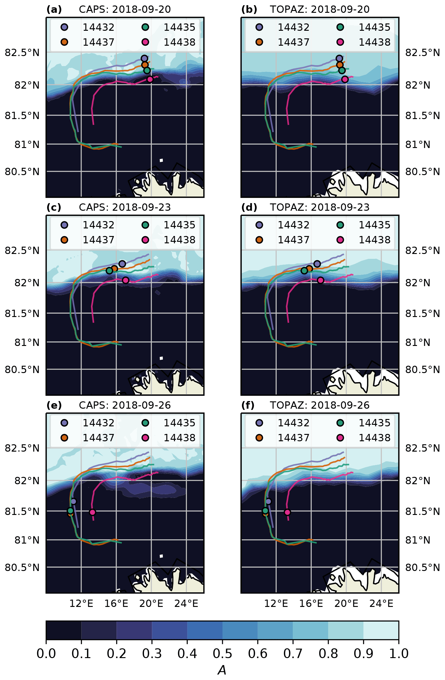
Figure 1Drifter tracks (–) and locations (o) at three different times during their respective trajectories. Filled contours of ice concentration are shown as calculated by CAPS (a, c, e) and TOPAZ (b, d, f). Drifter IDs, from furthest in the ice to nearest to ocean, are 14432 (blue), 14437 (orange), 14435 (green), and 14438 (red). Drifters exit the MIZ on approximately 25 September 2018 at 00:00 UTC.
The drifters are equipped with an inertial motion unit to measure the directional wave spectra and a GPS sensor which provides accurate measurements of the geographic location and time. The data are recorded on each drifter and sent via Iridium approximately every 3 h. The drifter velocities were calculated using the forward difference in geographic locations.
The drifters began transmitting data on 19 September 2018. Two drifters survived until 1 October 2018 (14435 and 14437), while the other two (14432 and 14438) stopped reporting on approximately 26 September 2018. From the available data it appears that each of the drifters stopped transmitting when they had left the MIZ (Fig. 1).
3.2 Ice–ocean prediction systems
The Canadian Arctic Prediction System (CAPS) is a coupled atmosphere–ice–ocean prediction system, with separate analyses for the atmosphere, ice, and ocean components, and a 48 h forecast is run four times a day at Environment and Climate Change Canada (ECCC) as part of the Year of Polar Prediction. The ice–ocean component is a ∘ coupled NEMO–CICE configuration as in Dupont et al. (2015). The ice–ocean component is coupled with an atmospheric model on a higher-resolution (3 km) grid. The dynamical core of the atmospheric component of CAPS is GEM (Global Environmental Multiscale), a non-hydrostatic model which solves the fully compressible Euler equations (Côté et al., 1998a, b; Girard et al., 2014).
TOPAZ is a coupled ice–ocean data assimilation system covering the North Atlantic and Arctic oceans (Sakov et al., 2012). TOPAZ represents the Arctic component of the Copernicus Marine Environment Monitoring Service (CMEMS) system (http://marine.copernicus.eu, last access: 20 May 2022). Atmospheric forcing is provided by the European Centre for Medium-range Weather Forecasting (ECMWF). The ocean component of TOPAZ is the Hybrid Coordinate Ocean Model (HYCOM), which is a hybrid model consisting of z-level vertical coordinates in the upper (mixed) layer and isopycnal coordinates below. The horizontal resolution is 12.5 km on a polar stereographic projection. The ocean model is coupled with a single thickness category ice model with elastic–viscous–plastic (EVP) rheology. Details can be found in Sakov et al. (2012) and Xie et al. (2017).
For all simulations, the wind forcing from CAPS is used. The CAPS model has a grid resolution of roughly 3 km, includes data assimilation, and is freely available. TOPAZ is forced by ECMWF IFS (Integrated Forecasting System) forecast data which have a spatial resolution of 0.1∘ (≃9 km) on a regular latitude–longitude grid (https://catalogue.marine.copernicus.eu/documents/PUM/CMEMS-ARC-PUM-002-ALL.pdf, last access: 20 May 2022). The choice of using only one of the wind forcing data sets is partially motivated by the ECMWF IFS forecast data requiring a licence but also allows for a simpler analysis to focus on the ice–ocean systems.
Snapshots of the ice concentration field (Fig. 1), as well as the along-track time series of ice concentration (Fig. 2), are calculated for both CAPS and TOPAZ. A consistent feature between the two ice concentrations is that after approximately 25 September 2018 both CAPS and TOPAZ predict that there is no ice at the drifter locations. This will allow us to test the model of Eq. (3) for an object that travels between ice and open water. There are also clearly some differences between the predicted ice concentrations which are most likely due to the different assimilation cycles of each model. While the analysis of the ice field in CAPS is updated for each forecast (every 12 h) the TOPAZ fields have a weekly analysis cycle, which could lead to the differences, especially for the two drifters which begin in lower ice concentrations (drifters 14435 and 14438).
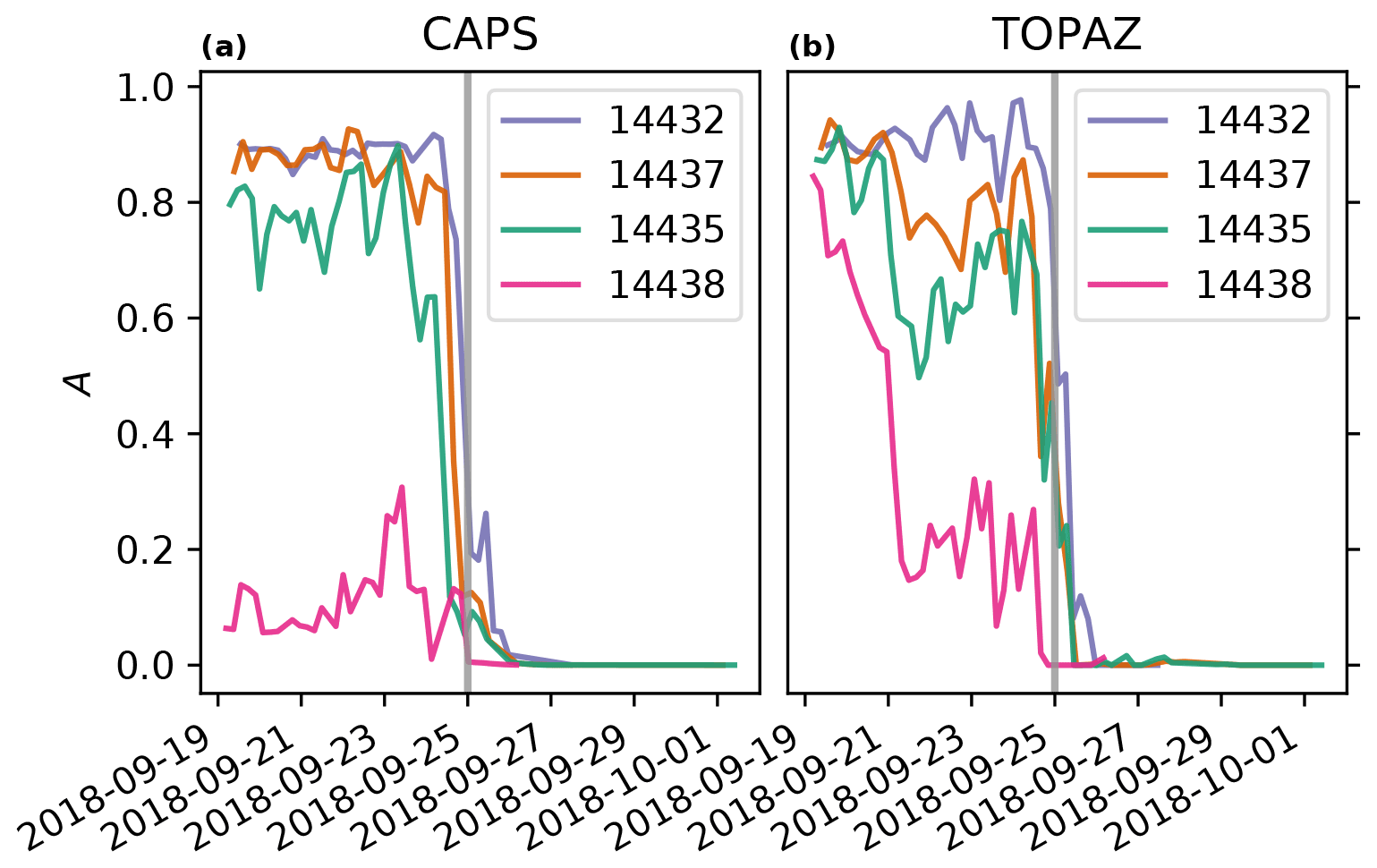
Figure 2Ice concentration interpolated to drifter tracks as calculated by (a) CAPS and (b) TOPAZ. The vertical grey line shows the approximate time (25 September 2018, 00:00 UTC) that the drifters leave the MIZ.
A comparison of the model and observed velocities for each drifter is shown in Fig. 3. Time series for ice, water, and wind (2 %) velocities, interpolated in time and space to available drifter observations, are shown. It is apparent from Fig. 3 that the observed drifter velocities are nearly always greater than either of the ice and water velocities from CAPS or TOPAZ. Ice and ocean velocities in CAPS vary in magnitude and direction more than those from TOPAZ. This is most likely due to ocean tides being included in CAPS, while these are not in TOPAZ as this region is known to have large diurnal tidal currents due to near-resonant, forced-topographic waves propagating around the Yermak Plateau (Hunkins, 1986; Padman et al., 1992).
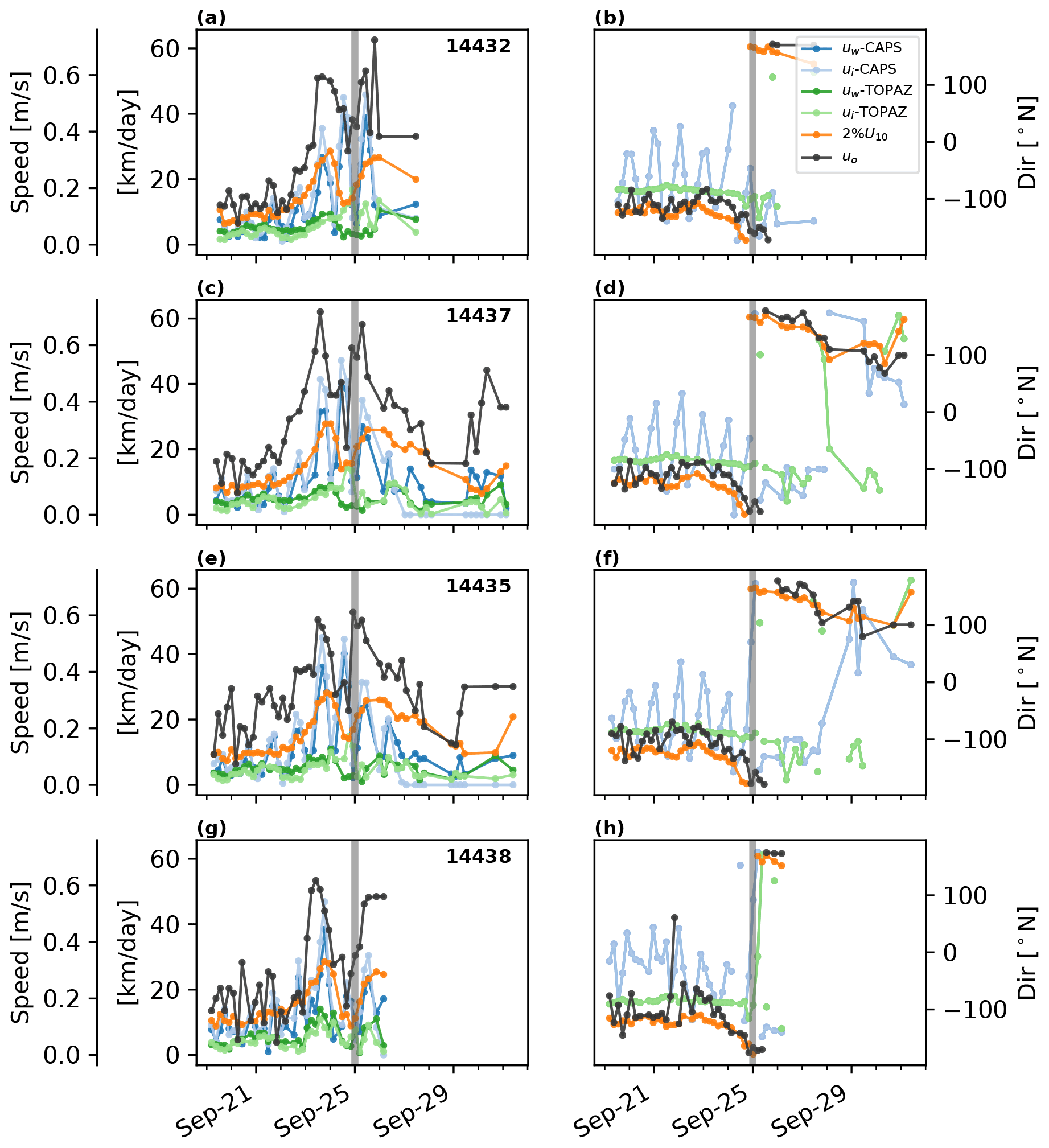
Figure 3Magnitude and direction of observed drifter velocities (uo, black) and predicted wind velocity (2 %; U10, orange), as well as ice (ui) and water velocities (uw), from CAPS (blue) and TOPAZ (green) interpolated to the drifter locations. The strong diurnal tidal current is clearly observed in CAPS but is absent from TOPAZ as this model does not include tides. The vertical grey line shows the approximate time when the drifters exit the MIZ.
3.3 Calculating leeway coefficients
As the drifters were deployed on ice floes, it is assumed that the drift of these ice floes in the MIZ can be given by Eq. (3). Ice drifters have been previously used by French-McCay et al. (2017) and Babaei and Watson (2020) in comparing transport equations with the drift of ice floes. However, even for ice floes over a wide range of ice concentrations, the weighting of Eq. (3) states that the ice floe will drift more like the water in low ice concentrations and more like the ice in high ice concentrations. The primary assumption for using the ice floes as a proxy for general transport is that the ice floe is small enough that inertial forces are negligible. Results using Eq. (3) will be compared with results using Eq. (1), as well as an ocean–leeway model (ki=0, αw=0.03) and an ice-only model (ki=1, αi=0).
The optimal leeway coefficients to be used in Eq. (3) are determined by minimizing the mean absolute error (MAE) between the observed and predicted velocities. The leeway coefficients are assumed to be constant in time and are a vector with both a downwind and crosswind component. It is also important to assess the sensitivity to these leeway coefficients, which is not trivial as the calculated MAE is a function of four variables since αi and αw are both vectors. To look at the sensitivity, 2-D slices are made through the 4-D MAE field to show the relative sensitivity for αi for a fixed αw and vice versa for αw for a fixed αi. The fixed points for these 2-D slices are selected from averaging the optimal leeway values for all the drifters and ice–ocean prediction systems.
3.4 Comparison of transport models in the MIZ
To compare the various transport models we simulate a series of 48 h trajectories for each drifter, transport model, and choice of ice–ocean prediction system. Lagrangian trajectories are simulated with MLDPn (Modèle Lagrangien de Dispersion de Particules d'ordre n), a Lagrangian dispersion model developed at ECCC (D'Amours et al., 2015) and adapted for aquatic use (Paquin et al., 2020). Virtual trajectories were launched every 12 h along the observed trajectory between 20 and 25 September 2018. This provides 44 virtual trajectories for each choice of transport model and ice–ocean prediction system.
Four different transport models are compared. First, the classic drift equation given by Eq. (1) with and leeway coefficients αw=0.03 and αi=0. These leeway coefficients are chosen for the method as they are typical values used in the MIZ (Nordam et al., 2019). Second is the more general Eq. (3) with the linear transfer function ki=A along with estimates for αw and αi from available data. The last two transport models consist of an ice-only (ki=1, αi=0) and an ocean-only transport model (ki=0, αw=0.03). The inclusion of a leeway term in the ocean-only model is to ensure consistency with Eq. (1) in the limiting case of no ice.
4.1 Ice and water leeway coefficients
The MAE between the observed drifter velocity and the model velocity from Eq. (3) is minimized for each drifter and choice of ice–ocean prediction system. The optimal leeway coefficients, as well as the MAE (in km d−1), are located in Table 1 for using the CAPS forcing and Table 2 for the TOPAZ forcing. To demonstrate the relative sensitivity to the choice of leeway coefficients, 2-D slices of the MAE contours are made through a fixed leeway coefficient; that is, the downwind and crosswind contours for the ice leeway are presented for a fixed water leeway and vice versa. Optimal leeway values are found to be approximately αw=0.03 and , and these are used for the constant leeway coefficients used for the MAE slices. No leeway angle is used for αw, but for αi an angle of −30∘ is found in which the negative implies clockwise rotation relative to the wind as we are using complex notation for our vectors. The MAEs for these fixed leeway coefficients are also shown in Tables 1 and 2, denoted MAE* in each table, and the difference is less than 1.5 km d−1 for each. Although not shown here, the MAE contours are qualitatively similar for different choices of fixed leeway coefficients with the primary difference being in the magnitude of the MAE.
Table 1Best fit for leeway coefficients using the CAPS forcing. MAE* is the mean absolute error using leeway values of and αw=0.03. Negative angles imply clockwise direction relative to wind.
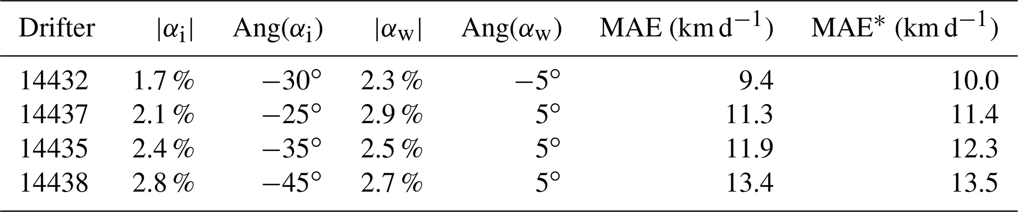
Table 2Best fit for leeway coefficients using the TOPAZ forcing. MAE* is the mean absolute error using leeway values of and αw=0.03. Negative angles imply clockwise direction relative to wind.
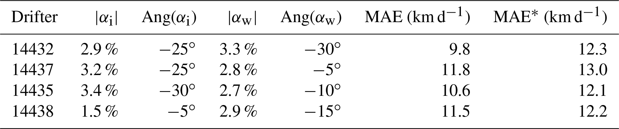

Figure 4Filled contours of MAE (in km d−1) between observed drift velocities and Eq. (3) for the along- and cross-wind components of αi with αw=0.03. The left column uses the CAPS forcing, and the right column uses TOPAZ forcing. The black dot shows the location of the MAE minimum, and the black contour line shows the MAE value within 1 km d−1 of the minimum. Each row is for an individual drifter in order from high ice concentration at the top to low ice concentration at the bottom. Sensitivity to the choice of αi is much greater in the high ice concentration than the low.
Filled contours of MAE for αi, with αw=0.03, for the downwind and crosswind components are shown in Fig. 4. The MAE contours for each drifter are very similar when using the CAPS data or the TOPAZ data. There is a clear sensitivity related to the ice concentration as the drifter furthest in the ice (14432) has the sharpest contour gradients in MAE and the drifter at the ice edge (14438) shows very little change in MAE for different values of αi. Not including drifter 14438, the optimal value for αi is approximately 0.02 and 30∘ to the right of the wind using the CAPS data and 0.03 and 30∘ to the right of the wind using the TOPAZ data. The difference between 0.02 and 0.03 is within the 1 km d−1 MAE contour, which is less than 10 % of the total MAE.
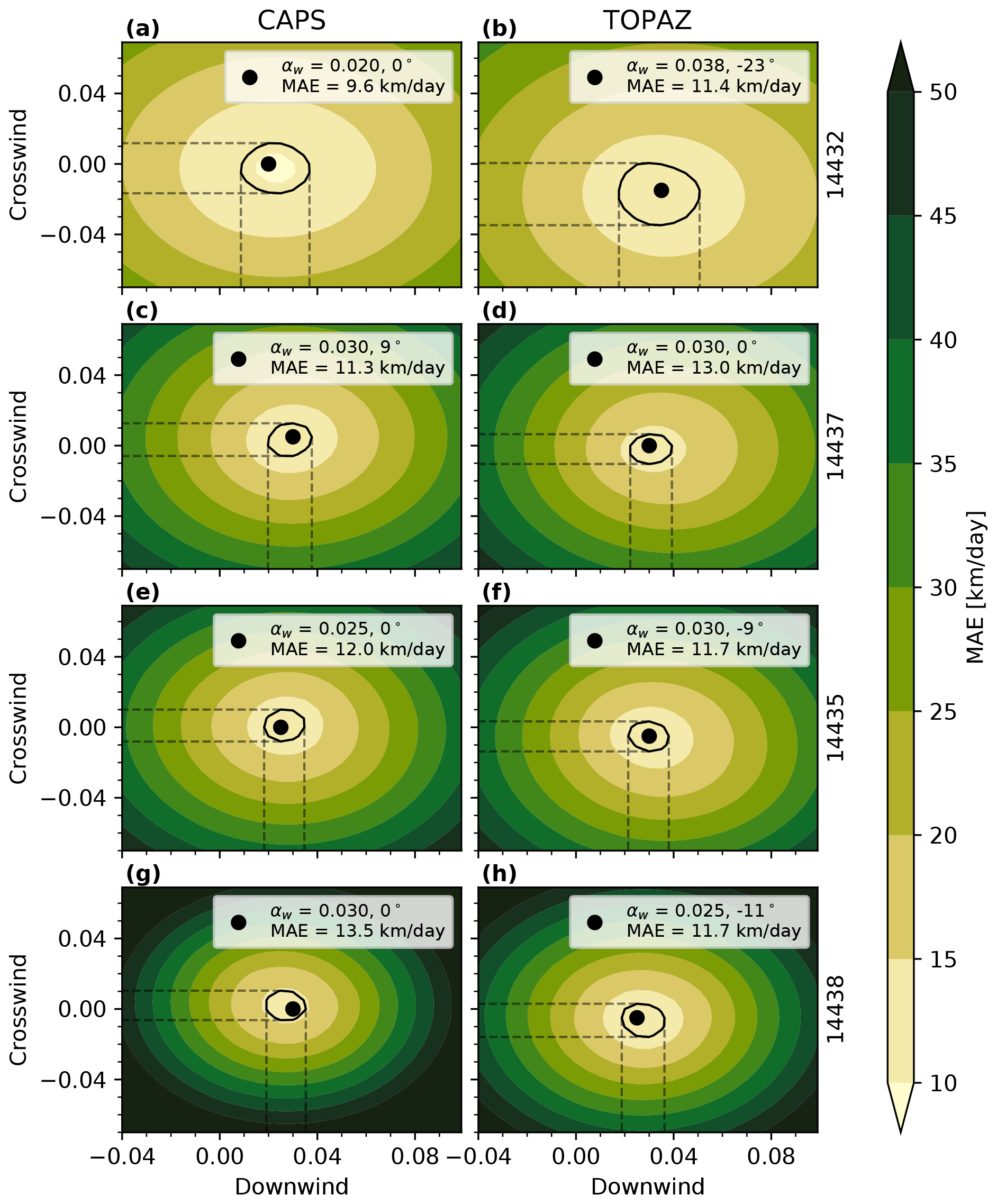
Figure 5Filled contours of MAE (in km d−1) between observed drift velocities and Eq. (3) for the along- and cross-wind components of αw with . The left column uses CAPS forcing, and the right column uses TOPAZ forcing. The black dot shows the location of the MAE minimum, and the black contour line shows the MAE value within 1 km d−1 of the minimum. Each row is for an individual drifter in order from high ice concentration at the top to low ice concentration at the bottom. Sensitivity to choice of αw is opposite to that of αi in Fig. 4 with less sensitivity in high ice concentration relative to low.
Filled contours of MAE for αw, with , for the downwind and crosswind components are shown in Fig. 5. Not surprisingly, the MAE contours in Fig. 5 have the opposite sensitivity as those in Fig. 4, with sharper contour gradients in MAE for the lowest ice concentration and MAE showing minimal sensitivity to the choice of αw in high ice concentration. Also, similar to Fig. 4, the MAE values in Fig. 5 are similar in magnitude when using either CAPS or TOPAZ data and range between 10 and 14 km d−1.
4.2 Short-term trajectory predictions
A few examples of the observed and modelled trajectories for each drifter can be found in Fig. 6. A more detailed presentation of the separation distance d after 48 h between the observed and modelled trajectories as a function of trajectory start time is located in Fig. 7. A summary of the mean and standard deviation of the separation distance d can be found in Table 3).
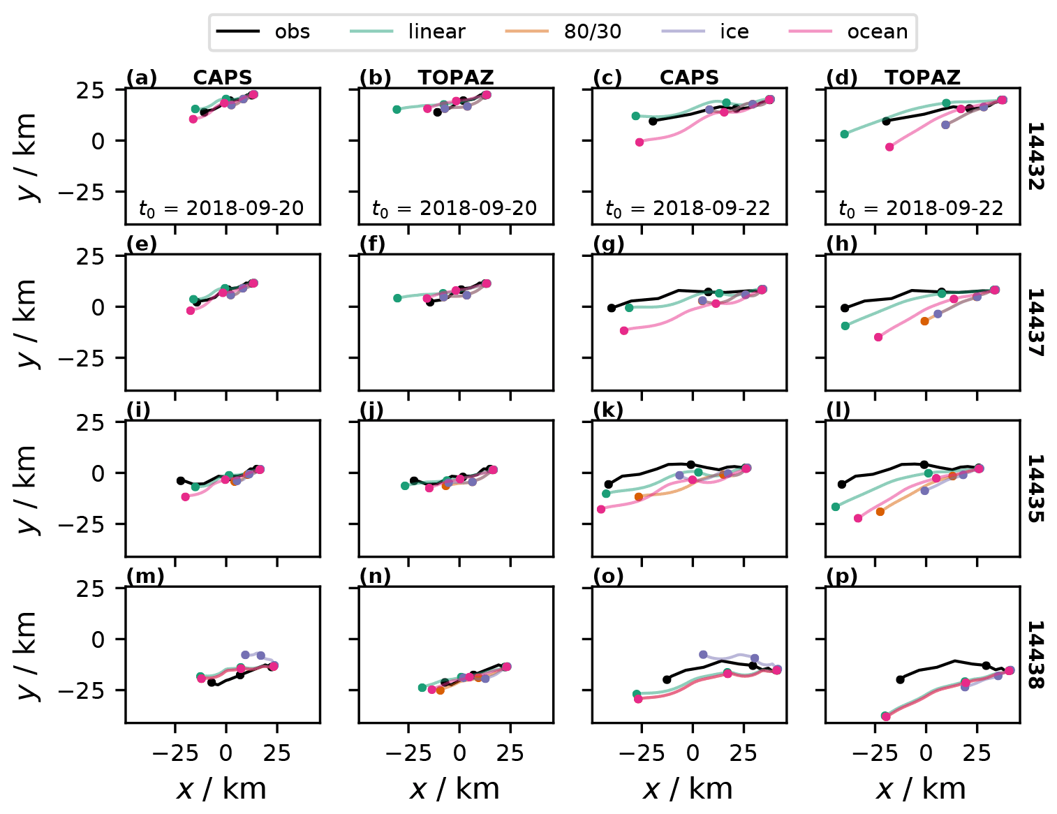
Figure 6Examples of observed and modelled 48 h trajectories. Each column corresponds to a combination of unique starting time and choice of ice–ocean forcing. Each row corresponds to a unique drifter. The dots represent locations at 24 h intervals. The x and y axes are in kilometers, and the choice of origin is arbitrary. The different predicted tracks are linear using Eq. (3), using Eq. (1), ice which uses only the ice velocities, and ocean which uses the ocean velocities plus 3 % leeway.
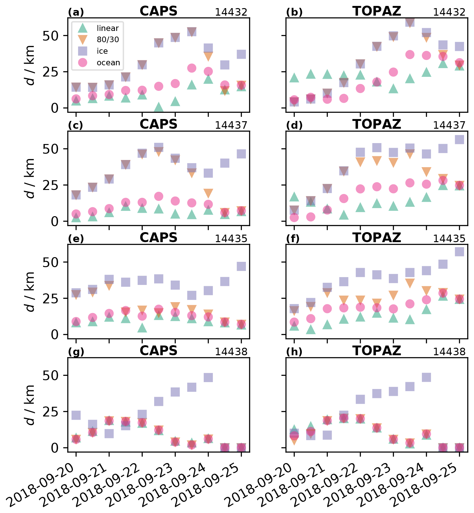
Figure 7Drifter separation (d in km) after 48 h. The horizontal axis denotes the start times for each simulation so that d is measured at 48 h after the time shown on the axis. The linear model corresponds to Eq. (3) and the model to (1), ice corresponds to the prediction with just ice velocities with no leeway, and ocean corresponds to the prediction with just ocean velocities plus 3 % leeway. The solid horizontal lines show the mean separation distance for each respective drift model. The inclusion of a leeway coefficient does reduce separation distance between observed and predicted trajectories, with the linear weighted model providing the best results.
Table 3Mean and standard deviation of separation distance d after 48 h (in km) from Fig. 7 for each drifter, forcing, and drift model.
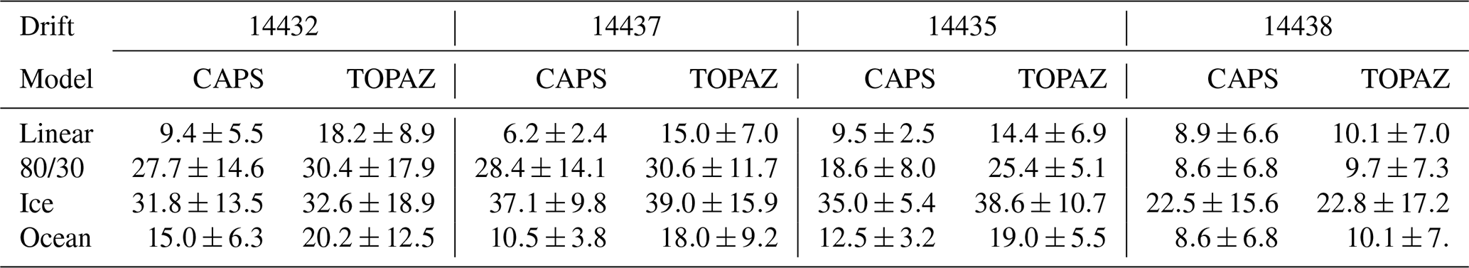
For the drifter furthest in the ice, 14432, and the drifter second furthest in the ice, 14437, the separation distance after 48 h is the smallest for forecasts beginning before 21 September, and this does not vary much with the choice of transport model or ice–ocean forcing (Fig. 7a and b). This changes rapidly after 21 September when the predicted trajectories using the and ice-only transport models perform poorly (large separation distance), while the linear model and ocean–leeway models do not produce such a dramatic change (Fig. 7a and b). The time when the transport models diverge corresponds with the increase in wind speed (Fig. 3a). As the ice-only and transport models do not have a leeway term (these two transport models are identical for A>0.8), the leeway term can improve 48 h trajectories when using ice–ocean prediction systems.
Drifter 14435, which is in an intermediate ice concentration, has a slightly different response than the previous two drifters in higher ice concentration. Similar to the other drifters, the leeway models (ocean–leeway, linear) have smaller trajectory errors than the non-leeway models (ice-only, for A>0.8). Where drifter 14435 is different is that the intermediate ice concentrations associated with this drifter trajectory, approximately 60 %–80 %, create two distributions in which the separation distances are sometimes similar to the ice-only model (Fig. 7e, before 21 September) and in which the distributions are more similar to those of the ocean–leeway model (Fig. 7e, after 21 September).
For the drifter in the lowest ice concentration, 14438, the , linear, and ocean–leeway models all have essentially the same trajectory error. As the ice concentrations, as provided by the model, are less than 0.3 (with the exception of TOPAZ before 21 September), it is expected that these three transport models should reproduce the same trajectory.
In general, the linear model using the best-fit leeway coefficients produces the smallest separation distance, as well as the least amount of variation as a function of simulation start time (Table 3). The ice-only transport model had the largest trajectory errors even though we are using drifters on ice floes as our proxy for transport in the MIZ. The ocean–leeway model had errors comparable to the linear model, and the model did not perform well in high ice concentration but did perform well in low ice concentration. These results were generally independent of the choice of CAPS or TOPAZ for the ice–ocean forcing. It would be interesting to expand the analysis to other ice–ocean prediction systems, for example, GOFS 3.1 (https://www7320.nrlssc.navy.mil/GLBhycomcice1-12/, last access: 20 May 2022), but this is beyond the scope of the current paper and is left to future research.
Presented here is a general equation to improve the transport of objects and material in waters with a mix of ice and ocean using ice–ocean prediction systems. The equation is a generalized leeway model and assumes a linear weighting of the ice and ocean velocities based on ice concentration and allows for a non-zero leeway, which can vary in both magnitude and direction, in both the ice and ocean components. Optimal leeway coefficients are calculated by minimizing the error between available observed drifter velocities in the MIZ and the model velocities calculated using ice–ocean velocities provided by two different coupled ice–ocean prediction systems: CAPS and TOPAZ. This general leeway model is inspired by the leeway model used for oil transport in ice-covered waters (Nordam et al., 2019), but we allow for a non-zero ice leeway to account for missing physics and uncertainties in the ice model.
By minimizing the error between the available observed and modelled trajectories, optimal values for the water and ice leeway coefficients, αw and αi, respectively, were determined. Optimal values for αw were found in the range , and for αi they were with a mean direction of 30∘ to the right of the wind. There are slightly larger values for αi using the TOPAZ data compared to the CAPS data. For αw, this range of values is consistent with 3 % required for the prediction of surface drifters (Sutherland et al., 2020) and oil spill modelling (Nordam et al., 2019). The αi values are curiously consistent with canonical values used for icebergs of about 2 % of the wind and 30∘ to the right (Leppäranta, 2011).
To assess the quality of the general leeway model we compared the trajectory difference between several transport models for a series of short-term (48 h) forecasts using the two different ice–ocean prediction systems (CAPS and TOPAZ). The general leeway model with the linear ki=A is used with the optimal leeway values of αw=0.03 and αi=0.02 and 30∘ to the right of the wind direction. This is compared with the transport equation used by the oil spill community, as well as an ice-only transport (ki=1, αi=0) and an ocean–leeway model (ki=0, αw=0.03). Results did not vary greatly between the two ice–ocean forcings. The linear general leeway model consistently had the smallest trajectory error for all four of the drifters. Somewhat surprisingly the ocean–leeway model consistently had the second smallest errors, even for the drifter in the highest ice concentration (14432). This is most likely due to the ice–ocean prediction systems being coupled so that the respective velocities will be strongly correlated in the MIZ when the internal ice stresses are small. The inclusion of the leeway is also key as it will compensate for missing physics, notably from surface waves which are not included in the ice–ocean prediction systems, and can compensate as well for any biases in the respective drag coefficients in the atmosphere–ice–ocean system. The model had mixed results and generally had smaller prediction errors for smaller ice concentrations than for large. This is most likely due to the lack of a leeway coefficient in the ice. The ice-only prediction had the largest errors, further emphasizing the importance of a leeway coefficient for the accurate short-term prediction of drift in the MIZ.
It is not obvious why the errors associated with calculating the leeway coefficients are similar between the CAPS and TOPAZ forcing (Figs. 4 and 5), while the separation errors are much smaller for CAPS than TOPAZ (Fig. 7). One likely explanation is due to the drifter observations being available every 3 h; hence velocities calculated using forward differences are also every 3 h, while CAPS and TOPAZ provide currents every hour. While averaging the CAPS and TOPAZ forcing would most likely reduce the magnitude of the MAE, it is not expected that this averaging would affect the relative sensitivity; i.e. the optimal leeway coefficients should not change. As CAPS includes tides and therefore has more variability at these frequencies than TOPAZ (Fig. 3), impacts on the magnitude of the MAE will probably be greater for CAPS than TOPAZ. However, simulation of the trajectories do not require the observed drifter velocities and should therefore be more accurate, i.e. the results in Fig. 7 and summarized in Table 3.
The inclusion of a leeway coefficient in the ice reduces the prediction error for our drifter trajectories. However, there is not enough information to ascertain whether this is due to missing physics in the prediction systems or correcting for biases that are correlated with the wind. More data would be welcome, and dedicated experiments which provide high-resolution observations, preferably hourly, are excellent for investigating short-term dynamics in the MIZ. Data sources, such as the International Arctic Buoy Program (IABP) (https://iabp.apl.uw.edu, last access: May 2022), could be another source of data for drift in the MIZ, but as these buoys are deployed in the pack ice they are dependent on the sea ice dynamics to reach the MIZ, provided they survive the journey, as well as other data products to determine whether they are in the MIZ or not. Attempting to use IABP could prove useful for understanding short-term dynamics, but given the unknowns mentioned above it is beyond the scope of this paper.
The likely physical explanation for including a leeway in the ice is due to surface waves, which are not uncommon in the MIZ (Rabault et al., 2020). The waves affect the motion of sea ice in two ways: first, there is an additional Lagrangian drift due to the presence of waves (the Stokes drift) and second, there is an additional force due to the attenuation of the surface waves, often called the radiation stress (Weber, 1987). This force will be in the direction of wave propagation, so since the waves are generally entering the ice from the ocean, this can cause the ice edge to compact (Sutherland and Dumont, 2018). There are also large uncertainties associated with the drag coefficients (Heorton et al., 2019) that could also be part of the leeway coefficient. It should also be emphasized that while the use of an ice leeway improved predictions in the MIZ, there is little reason to expect that this would be the case in the pack ice where internal stresses significantly impact the drift. In such a case, a more sophisticated expression for αi which depends on ice concentration such that αi→0 as A→1 would most likely be required and which also preserves some of the improvements shown in the MIZ.
The drifter data can be accessed at https://doi.org/10.21343/9p70-4q69 (Rabault, 2021). TOPAZ forecasts are available on the Copernicus Marine Environment Monitoring Service FTP server (https://resources.marine.copernicus.eu, last access: May 2022) at https://doi.org/10.48670/moi-00001 (CMEMS, 2022). CAPS ice–ocean forecasts and the atmospheric forecasts are available at https://doi.org/10.5281/zenodo.6576844 (Sutherland, 2022). Full forecast fields are available upon request from the corresponding author or the Meteorological Service of Canada at ec.dps-client.ec@canada.ca.
This article was written by GS with input from all co-authors. GS conceived of the idea, with feedback from all co-authors, and wrote the software for data analysis and production of figures. VdA, LRH, and MD contributed to preliminary data analysis. JR designed the drifters and was responsible for data collection and quality control. JR, LRH, and ØB contributed to drifter deployment.
The contact author has declared that neither they nor their co-authors have any competing interests.
Publisher's note: Copernicus Publications remains neutral with regard to jurisdictional claims in published maps and institutional affiliations.
Graig Sutherland and Mohammed Dabboor thank the Ocean Protection Plan (OPP) for funding and support of this work. Jean Rabault, Victor de Aguiar, Lars-Robert Hole, and Øyvind Breivik thank the Norwegian Research Council under the Nansen Legacy project (Arven etter Nansen) project for contributing to the development and deployment of the wave loggers. Jean Rabault thanks the Norwegian Research Council under the PETROMAKS2 scheme (project DOFI, grant number 28062) for funding. Lars-Robert Hole and Victor de Aguiar would also like to thank the Fram Centre MIKON Flagship program for support through the OSMICO project. Our warmest thanks go to the crew of R/V Kronprins Haakon for the time spent on the boat during the cruise and their help in deploying the drifters.
This research has been supported by the Norges Forskningsråd (grant no. 28062), the Environment and Climate Change Canada (Ocean Protection Plan), and the Norges Forskningsråd (grant no. 276730).
This paper was edited by Christian Haas and reviewed by two anonymous referees.
Babaei, H. and Watson, D.: A preliminary computational surface oil spill trajectory model for ice-covered waters and its validation with two oil spill events: A field experiment in the Barents Sea and an accidental spill in the Gulf of Finland, Mar. Pollut. Bull., 161, 111786, https://doi.org/10.1016/j.marpolbul.2020.111786, 2020. a
Breivik, Ø. and Christensen, K. H.: A combined Stokes drift profile under swell and wind sea, J. Phys. Oceanogr., 50, 2819–2833, 2020. a
Breivik, Ø., Allen, A. A., Maisondieu, C., and Roth, J. C.: Wind-induced drift of objects at sea: The leeway method, Appl. Ocean Res., 33, 100–109, 2011. a, b, c
Christensen, K. H., Breivik, Ø., Dagestad, K.-F., Röhrs, J., and Ward, B.: Short-Term Predictions of oceanic drift, Oceanography, 31, 59–67, 2018. a
CMEMS: Arctic Ocean Physics Analysis and Forecast (ARCTIC_ANALYSIS_FORECAST_PHYS_002_001_a), CMEMS [data set], https://doi.org/10.48670/moi-00001, last access: May 2022, updated daily. a
Cole, S. T., Toole, J. M., Lele, R., Timmermans, M.-L., Gallagher, S. G., Stanton, T. P., Shaw, W. J., Hwang, B., Maksym, T., Wilkinson, J. P., Ortiz, M., Graber, H., Rainville, L., Petty, A. A., Farrell, S. L., Richter-Menge, J. A., and Haas, C.: Ice and ocean velocity in the Arctic marginal ice zone: Ice roughness and momentum transfer, Elementa: Science of the Anthropocene, 5, 55, https://doi.org/10.1525/elementa.241, 2017. a
Côté, J., Desmarais, J.-G., Gravel, S., Méthot, A., Patoine, A., Roch, M., and Staniforth, A.: The operational CMC–MRB global environmental multiscale (GEM) model. Part II: Results, Mon. Weather Rev., 126, 1397–1418, 1998a. a, b
Côté, J., Gravel, S., Méthot, A., Patoine, A., Roch, M., and Staniforth, A.: The operational CMC–MRB global environmental multiscale (GEM) model. Part I: Design considerations and formulation, Mon. Weather Rev., 126, 1373–1395, 1998b. a, b
D'Amours, R., Malo, A., Flesch, T., Wilson, J., Gauthier, J.-P., and Servranckx, R.: The Canadian Meteorological Centre's atmospheric transport and dispersion modelling suite, Atmosphere-Ocean, 53, 176–199, 2015. a
Dupont, F., Higginson, S., Bourdallé-Badie, R., Lu, Y., Roy, F., Smith, G. C., Lemieux, J.-F., Garric, G., and Davidson, F.: A high-resolution ocean and sea-ice modelling system for the Arctic and North Atlantic oceans, Geosci. Model Dev., 8, 1577–1594, https://doi.org/10.5194/gmd-8-1577-2015, 2015. a, b, c
French-McCay, D. P., Tajalli-Bakhsh, T., Jayko, K., Spaulding, M. L., and Li, Z.: Validation of oil spill transport and fate modeling in Arctic ice, Arctic Sci., 4, 71–97, 2017. a, b, c
Girard, C., Plante, A., Desgagné, M., McTaggart-Cowan, R., Côté, J., Charron, M., Gravel, S., Lee, V., Patoine, A., Qaddouri, A., Roch, M., Spacek, L., Tanguay, M., Vaillancourt, P. A., and Zadra, A.: Staggered vertical discretization of the Canadian Environmental Multiscale (GEM) model using a coordinate of the log-hydrostatic-pressure type, Mon. Weather Rev., 142, 1183–1196, 2014. a, b
Heorton, H. D., Tsamados, M., Cole, S., Ferreira, A. M., Berbellini, A., Fox, M., and Armitage, T. W.: Retrieving sea ice drag coefficients and turning angles from in situ and satellite observations using an inverse modeling framework, J. Geophys. Res.-Oceans, 124, 6388–6413, 2019. a
Hibler III, W.: A dynamic thermodynamic sea ice model, J. Phys. Oceanogr., 9, 815–846, 1979. a, b, c, d
Hunkins, K.: Anomalous diurnal tidal currents on the Yermak Plateau, J. Mar. Res., 44, 51–69, 1986. a
Kirwan Jr., A., McNally, G., Chang, M., and Molinari, R.: The effect of wind and surface currents on drifters, J. Phys. Oceanogr., 5, 361–368, 1975. a
Leppäranta, M.: The drift of sea ice, Springer Berlin, Heidelberg, https://doi.org/10.1007/978-3-642-04683-4, 2011. a
Liu, Q., Rogers, W. E., Babanin, A., Li, J., and Guan, C.: Spectral modeling of ice-induced wave decay, J. Phys. Oceanogr., 50, 1583–1604, 2020. a
Lund, B., Graber, H. C., Persson, P., Smith, M., Doble, M., Thomson, J., and Wadhams, P.: Arctic sea ice drift measured by shipboard marine radar, J. Geophys. Res.-Oceans, 123, 4298–4321, 2018. a
Lüpkes, C., Gryanik, V. M., Hartmann, J., and Andreas, E. L.: A parametrization, based on sea ice morphology, of the neutral atmospheric drag coefficients for weather prediction and climate models, J. Geophys. Res.-Atmos., 117, D13112, https://doi.org/10.1029/2012JD017630, 2012. a, b
Masson, D. and LeBlond, P.: Spectral evolution of wind-generated surface gravity waves in a dispersed ice field, J. Fluid Mech., 202, 43–81, 1989. a
Nordam, T., Beegle-Krause, C., Skancke, J., Nepstad, R., and Reed, M.: Improving oil spill trajectory modelling in the Arctic, Mar. Pollut. Bull., 140, 65–74, 2019. a, b, c, d, e, f, g, h, i
Padman, L., Plueddemann, A. J., Muench, R. D., and Pinkel, R.: Diurnal tides near the Yermak Plateau, J. Geophys. Res.-Oceans, 97, 12639–12652, 1992. a
Paquin, J.-P., Lu, Y., Taylor, S., Blanken, H., Marcotte, G., Hu, X., Zhai, L., Higginson, S., Nudds, S., Chanut, J., Smith, G. C., Bernier, N., and Dupont, F.: High-resolution modelling of a coastal harbour in the presence of strong tides and significant river runoff, Ocean Dynamics, 70, 365–385, 2020. a
Rabatel, M., Rampal, P., Carrassi, A., Bertino, L., and Jones, C. K. R. T.: Impact of rheology on probabilistic forecasts of sea ice trajectories: application for search and rescue operations in the Arctic, The Cryosphere, 12, 935–953, https://doi.org/10.5194/tc-12-935-2018, 2018. a
Rabault, J.: Sea ice drifter trajectories from the Arven Etter Nansen Physical Process Cruise 2018, Norwegian Meteorological Institute [data set], https://doi.org/10.21343/9p70-4q69, 2021. a
Rabault, J., Sutherland, G., Gundersen, O., Jensen, A., Marchenko, A., and Breivik, Ø.: An open source, versatile, affordable waves in ice instrument for scientific measurements in the Polar Regions, Cold Reg. Sci. Technol., 170, 102955, https://doi.org/10.1016/j.coldregions.2019.102955, 2020. a, b
Rogers, W. E., Thomson, J., Shen, H. H., Doble, M. J., Wadhams, P., and Cheng, S.: Dissipation of wind waves by pancake and frazil ice in the autumn Beaufort Sea, J. Geophys. Res.-Oceans, 121, 7991–8007, 2016. a
Sakov, P., Counillon, F., Bertino, L., Lisæter, K. A., Oke, P. R., and Korablev, A.: TOPAZ4: an ocean-sea ice data assimilation system for the North Atlantic and Arctic, Ocean Sci., 8, 633–656, https://doi.org/10.5194/os-8-633-2012, 2012. a, b, c, d
Schweiger, A. J. and Zhang, J.: Accuracy of short-term sea ice drift forecasts using a coupled ice-ocean model, J. Geophys. Res.-Oceans, 120, 7827–7841, 2015. a
Spaulding, M. L.: State of the art review and future directions in oil spill modeling, Mar. Pollut. Bull., 115, 7–19, 2017. a, b
Squire, V. A.: Ocean wave interactions with sea ice: a reappraisal, Annual Rev. Fluid Mech., 52, 37–60, 2020. a, b
Sutherland, G.: graig-sutherland/transport-miz-tc: Software and Data for MIZ Transport by Sutherland et al., TC, 2022 (Version v1), Zenodo [data set], https://doi.org/10.5281/zenodo.6576844, 2022. a
Sutherland, G., Soontiens, N., Davidson, F., Smith, G. C., Bernier, N., Blanken, H., Schillinger, D., Marcotte, G., Röhrs, J., Dagestad, K.-F., Christensen, K. H., and Breivik, Ø.: Evaluating the Leeway Coefficient of Ocean Drifters Using Operational Marine Enviornmental Prediction Systems, J. Atmos. Ocean. Tech., 37, 1943–1954, 2020. a, b, c
Sutherland, P. and Dumont, D.: Marginal ice zone thickness and extent due to wave radiation stress, J. Phys. Oceanogr., 48, 1885–1901, 2018. a
Tsamados, M., Feltham, D. L., Schroeder, D., Flocco, D., Farrell, S. L., Kurtz, N., Laxon, S. W., and Bacon, S.: Impact of variable atmospheric and oceanic form drag on simulations of Arctic sea ice, J. Phys. Oceanogr., 44, 1329–1353, 2014. a
Venkatesh, S., ElTahan, H., Comfort, G., and Abdelnour, R.: Modelling the behavior of oil spills in ice-infested waters, Atmosphere-Ocean, 28, 303–329, 1990. a, b
Weber, J. E.: Wave attenuation and wave drift in the marginal ice zone, J. Phys. Oceanogr., 17, 2351–2361, 1987. a, b, c
Weber, J. E.: Virtual wave stress and mean drift in spatially damped surface waves, J. Geophys. Res.-Oceans, 106, 11653–11657, 2001. a
Wilkinson, J. and Wadhams, P.: A salt flux model for salinity change through ice production in the Greenland Sea, and its relationship to winter convection, J. Geophys. Res.-Oceans, 108, 3147, https://doi.org/10.1029/2001JC001099, 2003. a
Wu, J.: Sea-surface drift currents induced by wind and waves, J. Phys. Oceanogr., 13, 1441–1451, 1983. a, b
Xie, J., Bertino, L., Counillon, F., Lisæter, K. A., and Sakov, P.: Quality assessment of the TOPAZ4 reanalysis in the Arctic over the period 1991–2013, Ocean Sci., 13, 123–144, https://doi.org/10.5194/os-13-123-2017, 2017. a