the Creative Commons Attribution 4.0 License.
the Creative Commons Attribution 4.0 License.
 | 17 May 2022
The sensitivity of landfast sea ice to atmospheric forcing in single-column model simulations: a case study at Zhongshan Station, Antarctica
Fengguan Gu
Qinghua Yang
Frank Kauker
Changwei Liu
Guanghua Hao
Chao-Yuan Yang
Jiping Liu
Petra Heil
Xuewei Li
Bo Han
Single-column sea ice models are used to focus on the thermodynamic evolution of the ice. Generally, these models are forced by atmospheric reanalysis in the absence of atmospheric in situ observations. Here we assess the sea ice thickness simulated by a single-column model (ICEPACK) with in situ observations obtained off Zhongshan Station for the austral winter of 2016. In the reanalysis, the surface air temperature is about 1 ∘C lower, the total precipitation is about 2 mm d−1 greater, and the surface wind speed is about 2 m s−1 higher compared to the in situ observations. We designed sensitivity experiments to evaluate the simulation bias in sea ice thickness due to the uncertainty in the individual atmospheric forcing variables. Our results show that the unrealistic precipitation in the reanalysis leads to a bias of 14.5 cm in sea ice thickness and 17.3 cm in snow depth. In addition, our data show that increasing snow depth works to gradually inhibit the growth of sea ice associated with thermal blanketing by the snow due to changing the vertical heat flux. Conversely, given suitable conditions, the sea ice thickness may grow suddenly when the snow load gives rise to flooding and leads to snow-ice formation. However, there are still uncertainties related to the model results because superimposed ice and snowdrift are not implemented in the version of the ice model used and because snow-ice formation might be overestimated at locations with landfast sea ice.
- Article
(2298 KB) - Full-text XML
- BibTeX
- EndNote


Sea ice plays an essential role in the global climate system by reflecting solar radiation and regulating the heat, moisture, and gas exchanges between the ocean and the atmosphere. In contrast to the rapid decline of sea ice extent and volume in the Arctic (Stroeve et al., 2012; Lindsay and Schweiger, 2015), satellite observations have shown a slight increase in the yearly mean area of Antarctic sea ice since the late 1970s (Parkinson and Cavalieri, 2012) followed by a rapid decline from 2014 (Parkinson, 2019) and a renewed increase in the most recent years (Chemke and Polvani, 2020). Although the sudden decline in Antarctic sea ice is yet to be attributed (Parkinson, 2019), the spatial pattern of Antarctic sea ice changes is suggested to be primarily caused by changes in the atmospheric forcing. For example, the rapid ice retreat in the Weddell Sea from 2015 to 2017 has been associated with the intensification of northerly wind (Turner et al., 2017), while the phase of the southern annular mode (SAM) significantly modulates the sea ice in the Ross Sea and elsewhere, especially in November 2016 (Stuecker et al., 2017; Schlosser et al., 2018; G. Wang et al., 2019).
Landfast sea ice, the immobile fraction of the sea ice, is mainly located near coastal regions of Antarctica, and its change is assumed to be indicative of the evolution of total Antarctic sea ice (Heil et al., 1996; Heil, 2006; Lei et al., 2010; Q. Yang et al., 2016). Unlike drifting sea ice, the change in landfast sea ice is dominated by thermodynamic processes which single-column sea ice models can capture well (Heil et al., 1996; Lei et al., 2010; Y. Yang et al., 2016; Zhao et al., 2017; Liu et al., 2022). Furthermore, a single-column sea ice model is a useful tool to evaluate the impacts of different atmospheric forcings on the sea ice evolution because of the relatively simple structure of the physical processes (Cheng et al., 2013; C. Wang et al., 2019; Merkouriadi et al., 2020). In this study, a state-of-the-art single-column sea ice model, ICEPACK, is chosen to investigate the sensitivity of landfast sea ice to atmospheric forcing for the region off Zhongshan Station in Prydz Bay, East Antarctica (Fig. 1).
Due to the lack of in situ observations, the majority of sea ice studies, especially for the Antarctic, rely on numerical models. Realistic atmospheric forcing is critical for reliable model simulations. Although being criticized for significant deviations from in situ observations (Bromwich et al., 2007; Vancoppenolle et al., 2011; Wang et al., 2016; Barthélemy et al., 2018), atmospheric reanalysis data are assumed to offer reasonable atmospheric forcing for large-scale sea ice models for the Antarctic (Zhang, 2007; Massonnet et al., 2011; Zhang, 2014; Barthélemy et al., 2018). Previous studies reported a large spread between four global atmospheric reanalysis products and in situ observations in the Amundsen Sea Embayment (Jones et al., 2016). Moreover, studies showed that directly using atmospheric reanalysis as forcing for models causes significant biases in the Arctic sea ice simulations (Lindsay et al., 2014; C. Wang et al., 2019). Similar results, accentuated by the sparseness of atmospheric observations entering the reanalysis, can be foreseen for Antarctica. Therefore, the atmospheric forcing needs to be evaluated carefully before simulating Antarctic sea ice. To our knowledge, few studies have given a quantitative evaluation of the effect of different atmospheric forces on sea ice simulations in Antarctica.
The coastal landfast sea ice in Prydz Bay is generally first-year ice. It usually fractures and is exported or melts out completely between December and the following February, and refreeze occurs from late February onwards (Lei et al., 2010). This seasonal cycle is representative of Antarctic landfast sea ice. This study aims to evaluate the contributions of the various atmospheric forcing variables on landfast sea ice growth. The snow cover exerts influence on the evolution of the vertical sea ice–snow column via a number of mechanisms, including the formation of snow ice added by flooding (Leppäranta, 1983), superimposed ice (Kawamura et al., 1997), and insulating impact (Massom et al., 2001). Understanding the snow depth is a primary concern here.
Two sets of atmospheric forcing have been chosen. The first is spatially interpolated ERA5 onto the location of the observation site, and the second is using in situ atmospheric observations. It is well known that the simulation biases of numerical models are introduced through many shortcomings, including unrealistic surface boundary conditions (here: atmospheric forcing), imperfect physical process formulations, and computational errors. Understanding the uncertainty in sea ice simulations, as well as the sea ice response pattern to atmospheric forcing due to imperfect surface boundaries, is a prerequisite for successful simulations and needs to be assessed first.
This study is arranged as follows: the in situ observations, the numerical model, and the reanalysis are introduced in Sect. 2. The main results are given in Sect. 3, focusing on different kinds of atmospheric forcing on sea ice and snow. Shortcomings, discussions, and conclusions follow in Sects. 4, 5, and 6.
2.1 Meteorological observations
The site of sea ice observations is located in the coastal area off Zhongshan Station (69∘22′ S, 76∘22′ E; Fig. 1), East Antarctica. The meteorological data were collected at a year-round manned weather observatory run at Zhongshan Station in 2016, which is 1 km inland from the sea ice observation site and 15 m above sea level. Snowfall is measured every 12 h at the Russian Progress II station (located ∼1 km to the southeast of Zhongshan Station). The short- and longwave radiation fluxes were measured every minute with a net radiometer mounted 1.5 m above the surface on a tripod (Q. Yang et al., 2016). Other meteorological variables are available as hourly data, including 2 m air temperature (T2 m), surface pressure (Pa), specific humidity (calculated from dew-point temperature and Pa), potential temperature (calculated from T2 m and Pa), air density (calculated by T2 m and Pa), and 10 m wind speed (U10) (Hao et al., 2019, 2020; Liu et al., 2020).

Figure 1Location of landfast sea ice surface measurements near Zhongshan Station. The solid triangle denotes the observation site, and the solid circle marks Zhongshan Station. The color on the left represents the terrain.
2.2 Sea ice thickness measurement
A thermistor-chain unit developed by Taiyuan University of Technology (TY) was used to measure sea ice thickness in austral winter 2016. This unit is composed of two parts: the control unit and the thermistor chain. The controller initiates data acquisitions and records and stores the temperature measurements. The thermistor chain is 3 m long with 250 equidistant thermistors. Their sensitivity is 0.063 ∘C, and the measurement accuracy is ±0.1 ∘C. The thermistor chain simultaneously records the vertical temperature profile across the near-surface atmosphere, snow cover, sea ice, and surface seawater. The measurement frequency is hourly. Details about the instruments can be found in Hao et al. (2019).
Snow thickness close to the thermistor unit is measured weekly using a ruler with an accuracy of ±0.2 cm. Sea ice thickness is measured with a ruler through a drill hole (5 cm diameter) weekly. The measurement accuracy is ±0.5 cm. The average thickness obtained from three close-by sites is retained. Sea-surface temperature and sea-surface salinity are measured in the drill holes weekly using a Cond 3210 SET1 (Hao et al., 2019).
2.3 Atmospheric reanalysis data
The European Centre for Medium-range Weather Forecasts (ECMWF) released ERA5, the new reanalysis product, in 2017, which is updated in near real time (Hersbach and Dee, 2016; Hersbach et al., 2020). The complete ERA5 data set, extending back to 1950, has been available to the end of 2019 during this study. Compared with the popular ERA-Interim reanalysis, there are several significant improvements in ERA5, including much higher resolutions (both spatially and temporally). ERA5 has global coverage with a horizontal resolution of 31 km by 31 km at the Equator and 10 km by 31 km at the latitude of Zhongshan Station. The ERA5 resolves the vertical atmosphere profile using 137 vertical pressure levels from the surface up to a geopotential height of 0.01 hPa. ERA5 provides hourly analysis and forecast fields and applies a four-dimensional variational data assimilation system (4D-var). ERA5 includes various reprocessed quality-controlled data sets, for example, the reprocessed version of the Ocean and Sea Ice Satellite Application Facilities (OSI SAF) sea ice concentration (Hersbach and Dee, 2016; Hersbach et al., 2020).
For comparison and evaluation against the observations in this study, gridded data from ERA5 has been bilinearly interpolated to the observation site (detailed in Sect. 2.1). Directly using atmospheric forcing from coarse grid cells to interpolate to the observation site, although widely accepted in previous studies (e.g., Urraca et al., 2018; C. Wang et al., 2019), may cause errors. We have checked the performance of ERA5 and found that the spatial difference of surface atmospheric variables around the observation site is relatively small, indicating the choice of interpolation techniques will not affect the conclusion of this study.
2.4 ICEPACK
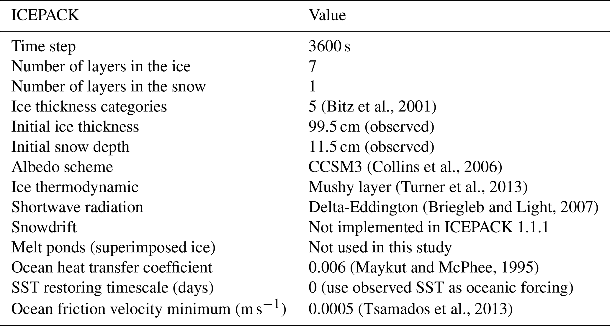
ICEPACK is a column-physics component of the Los Alamos Sea Ice Model (CICE) V6 and is maintained by the CICE Consortium. ICEPACK incorporates column-based physical processes that affect the area and thickness of sea ice. It includes several options for simulating sea ice thermodynamics, mechanical redistribution (ridging), and associated area and thickness changes. In addition, the model supports several tracers, including ice thickness, enthalpy, ice age, first-year ice area, deformed ice area and volume, melt ponds, and biogeochemistry (Hunke et al., 2019). ICEPACK Version 1.1.1 was used in this study, and detailed options of physical parameterizations and model settings for ICEPACK are summarized in Table 1. We employ ICEPACK to distribute the initial ice thickness to each ice thickness category using a distribution function:
where h is the initial ice thickness, Hi is the prescribed ice thickness category (0–0.6, 0.6–1.4, 1.4–2.4, 2.4–3.6, and above 3.6 m; same as for Arctic simulations), and N is the number of ice thickness categories.
Table 1Detailed options of physical parameterizations and model settings for ICEPACK. SST signifies sea surface temperature.
The atmospheric forcing for the ICEPACK model consists of observations of downward short- and longwave radiation, 2 m air temperature, specific humidity, total precipitation, potential temperature, 2 m air density, and 10 m wind speed. The oceanic forcing includes sea surface temperature, sea surface salinity, and oceanic mixed layer depth. The period concerned in this study is from 22 April, when observed sea ice generally starts to grow, to 22 November 2016. Since there are no observations of the ocean's mixed-layer depth, we set it to 10 m based on a previously published study (Zhao et al., 2019).
3.1 Surface atmospheric conditions near the observation site
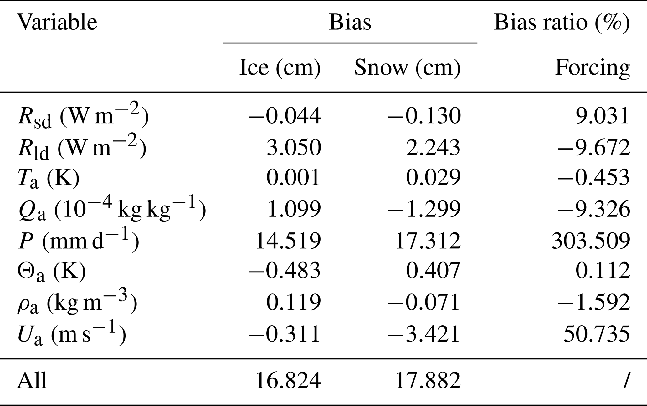
First, we compare the eight atmospheric variables used to force ICEPACK (surface downward shortwave radiation (Rsd), surface downward longwave radiation (Rld), surface air temperature (Ta), specific humidity (Qa), precipitation (P), air potential temperature (Θa), air density (ρa), and wind speed (Ua) with the respective in situ observations). Table 2 lists the bias (reanalysis minus observation), bias ratio (ratio between the bias and the observation value), the mean value of the in situ observations (Mean_Obs), the correlation coefficient (Corr.), and the root-mean-square deviation (RMSD) between the interpolated ERA5 data and the observations. In general, all eight variables from the two sources closely follow each other (Corr. >0.85), except for P and Ua. In this study, the main attention is on the atmospheric variables Ta, P, and Ua for three reasons. (1) Previous studies (Cheng et al., 2008; Wang et al., 2015) have shown that from all atmospheric forcing variables, uncertainties in Ta, P, and Ua exert a significant impact on the sea ice thickness (Cheng et al., 2008). (2) Surface wind may affect the snow cover in two ways: sublimation due to surface turbulent heat flux (Fairall et al., 2003; Gascoin et al., 2013) and the snowdrift process (Thiery et al., 2012). (3) P and Ua from the reanalysis have the largest bias ratio compared to the in situ observations.
The timing of daily variations in Ta is well represented by ERA5, especially for strong cooling events (Fig. 2a). However, ERA5 tends to underestimate warm events by a few degrees, as well as cold events during which differences exceeding 10 ∘C may occur (Fig. 2d). During the entire observation period in 2016, Ta from ERA5 was 1.2 ∘C lower than the in situ observations. Also, previous studies reported similar disagreement in Ta between observations and reanalysis in Antarctica (Bracegirdle and Marshall, 2012; Fréville et al., 2014). The cold bias of Ta in the reanalysis was suggested to be caused by the ice surface schemes that cannot accurately describe the ice–atmosphere interactions of strongly stable stratified boundary layers that are frequent in Antarctica.
Table 2Comparison of atmospheric forcing between ERA5 reanalysis and in situ observations.

The reanalyzed variable with the largest bias ratio from the observations is precipitation (Fig. 2b). Hourly precipitation from ERA5 was accumulated into daily data and compared with the nearest available daily precipitation records from the Progress II station. The maximum daily mean precipitation can reach 19.1 mm d−1 (11 July 2016), with an average of 0.66 mm d−1 from 29 April to 22 November 2016. While ERA5 captures the main precipitation events, it significantly overestimated the magnitude of precipitation events, especially in July. In this month, the mean precipitation rate from ERA5 is 5.83 mm d−1, while the observed is only 1.42 mm d−1. From April to November, the accumulated precipitation from ERA5 is about 300 % larger than that in the in situ observations. Nevertheless, using precipitation from Progress II for Zhongshan Station may be questioned because of the distance of about 1 km to Zhongshan Station. Moreover, the snowdrift due to strong surface wind can affect the precipitation observations and the local accumulated snow mass, which may further cause a significant bias in snow depth between simulation and observations.

Figure 2Time series of daily (a) surface air temperature, (b) precipitation rate, and (c) wind speed (10 m above the surface). The ERA5 reanalysis data are indicated as red lines. Observations are marked by black lines. Panels (d–f) show the difference (marked by “D”) between ERA5 and the observations (ERA5-observation). The differences are marked by blue lines. The gray lines denote the zero line.
The observed Ua varied from 0.01 to 12.3 m s−1 with an average of 4.2 m s−1 (Fig. 2c). ERA5 captured well the daily and seasonal variation in Ua, but an overestimation of 2.1 m s−1 should be noted, mainly when observed Ua>5 m s−1. One explanation for such an overestimation is that the numerical model underlying ERA5 cannot represent the surface roughness and the katabatic wind in a region with complex orography (Tetzner et al., 2019; Vignon et al., 2019).
3.2 Simulation forced by observed in situ atmospheric variables
The simulation bias of sea ice thickness and snow depth is impacted by many aspects, including unrealistic atmospheric and oceanic forcing and shortcomings in the applied numerical model. In this study, we mainly focus on the influence of imperfect atmospheric forcing.
The sea ice thickness (Obs) measured through a drill hole increases from 29 April (100±2 cm) to 25 October (172±2 cm), remaining level from there on (Fig. 3a). The ice thickness deduced from the TY (Obs_TY) thermistor-chain buoy shows a similar result: sea ice thickness increased from 106 cm on 22 April to 171 cm on 17 November. In November, the sea ice thickness (Obs and Obs_TY) is stationary, indicating a thermodynamic equilibrium between heat loss to the atmosphere and heat gain from the ocean (Q. Yang et al., 2016; Hao et al., 2019).
When forced by atmospheric in situ observations (Sim_Obs), the simulated sea ice thickness agrees well with the observed thickness with a mean bias of less than 1 cm over the growing season. We attribute the excellent simulation result to the fact that the seasonal evolution of landfast sea ice is driven mainly by thermal processes, which ICEPACK captures well.
The average snow depth from observations is 17 cm during the ice-growth season, with low snow depth measured before 11 July (Fig. 3b). After that, the snow depth increases rapidly up to about 37 cm, associated with a precipitation event arising from a single synoptic system. Then it decreases below the seasonal mean (Obs_mean), followed by two secondary maxima (>25 cm) on 8 September and 18 October.
The snow depth in Sim_Obs tracks the observations closely before 2 August (Fig. 3b). Then, the observed snow depth decreased quickly from about 30 cm to about 10 cm, while the Sim_Obs snow depth continued to increase gradually until the onset of surface melting in November. We attribute the observed quick decrease in snow depth to the effect of the snowdrift because the surface wind stayed above 5 m s−1 for most of August (Fig. 2c), giving rise to snowdrift, a process not implemented in the version of ICEPACK used here. The snowdrift might cause a significant spatial difference in accumulated snow patterns (Liston et al., 2018), which may be responsible for the large deviation in snow depth between Sim_Obs and observations. In addition, Sim_Obs underestimated the snow depth on 11 July. As discussed above, using nonlocal observed precipitation from Progress II should be questioned.
Using observed meteorological variables as atmospheric forcing in ICEPACK produced unreliable snow depth, while the sea ice thickness was in reasonably good agreement. In other words, the enormous bias in snow depth seems to have little effect on the sea ice thickness in the simulation. This counter-intuitive finding is of great interest to us because it disobeys the general realization that the snow layer significantly modifies the energy exchange on top of the sea ice. Potential causes for this result will be discussed later.
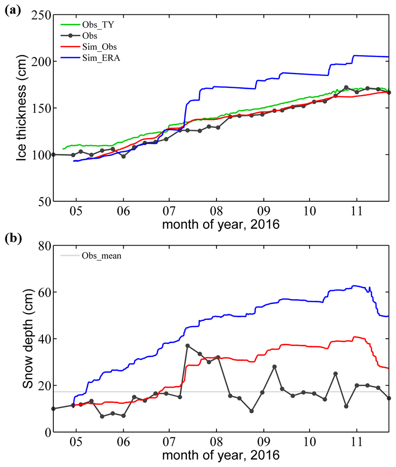
Figure 3Time series of (a) sea ice thickness and (b) snow depth during the freezing season. Solid black lines with black points show the observations from the drill hole (Obs). Solid green lines show the ice thickness derived from the TY buoy (Obs_TY). Solid red lines show the simulation results under in situ atmospheric forcing (Sim_Obs), and solid blue lines are simulation results under ERA5 forcing (Sim_ERA). In (b), the solid gray line shows the seasonal mean snow depth observations (Obs_mean).
3.3 Simulation forced by ERA5 atmospheric variables
When forced by ERA5 (Sim_ERA), the simulated sea ice thickness shows significant deviations from observations (Fig. 3a). The deviation is only about 1 cm before 11 July, when a heavy precipitation event (∼19 mm d−1) happened. After the precipitation episode, the offset in the sea ice thickness between Sim_ERA and observations was almost constant, about 33 cm.
In contrast to sea ice thickness, the precipitation from ERA5 causes an overestimation in snow depth for the entire simulation period. The snow depth from Sim_ERA is much greater than observations, even before 11 July (Fig. 3b). During the heavy precipitation event (Fig. 2b), the observed snow depth increased from 20 cm to about 40 cm. Although the precipitation rate from ERA5 (∼40 mm d−1) is 2 times larger than the observations, it caused little response in the simulated snow depth. The snow depth increase is near-linear, from about 10 cm to almost 60 cm.
3.4 Sensitivity analysis
To determine which atmospheric variables, including Ta, P, and Ua, are the most crucial in the sea ice simulation, we designed a set of sensitivity simulation experiments named SEN1. The simulation under the forcing from the in situ observed atmospheric variables is the control experiment and is named Sim_Obs. In each experiment of SEN1, one atmospheric variable is replaced by the corresponding variable from ERA5, while all others are identical to those of the control experiment. In Table 3, the averaged bias between the simulation and the observations of the outputs (ice thickness and snow depth) and the bias ratio of forcing atmospheric variables are listed separately.
Table 3Bias of ice thickness, snow depth, and bias ratio for each forcing variable from Table 2. “All” means using the full set of ERA5 atmospheric forcing.
To determine the sensitivity of sea ice and snow depth near Zhongshan Station to atmospheric forcing, we designed a set of numerical experiments named SEN2. In the control run, the forcing of the simulation directly used the means of observed atmospheric variables (Mean_Obs in Table 4). For a specific atmospheric variable, we build a set of sensitive runs. The focused atmospheric variable changed from its mean (Range in Table 4), and other variables are the same as the control run. Considering the actual range of each observed variable on an interannual scale (M. Van Den Broeke et al., 2004; Jakobs et al., 2020; Roussel et al., 2020), we set the maximum change in Ta, Θa, and ρa to 2 % and other atmospheric variables to 50 %. Then, we concluded the sensitivity of sea ice and snow to each atmospheric forcing from its corresponding sensitive runs. Because sea ice and snow depth show a quasi-linear response to the change in each specific atmospheric forcing (not shown), the choice of the variable's range will not alter the sensitivity results.
Table 4The atmospheric forcing (Mean_Obs for the control run and Range for the sensitive run) and sensitivity from SEN2.

Comparing the individual biases in Table 3, it turns out that P and Rld from ERA5 contribute to the bias in sea ice thickness most strongly. For snow depth, P, Ua, and Rld contribute the most. In Table 4, the sensitivity of ice thickness and snow depth to each atmospheric variable are listed. Comparing the individual sensitivity, it turns out that the sea ice thickness and snow depth are most sensitive to Ta and Θa. However, Ta from ERA5 is close to the in situ observations, so the simulated sea ice thickness and snow depth are hardly impacted (Table 3). The results from SEN1 reveal that the overestimation of P in ERA5 is the primary source of the overestimation of sea ice thickness and snow depth, even with less sensitivity to precipitation (Table 4).
To clarify the effect of specific forcing further, we replaced the x forcing in Sim_Obs with the corresponding ERA5 variable and named it Sim_ERA_x. Compared with Sim_Obs, Sim_ERA_P overestimates the snow depth from May onwards (Fig. 4b) and shows a significant positive bias in sea ice thickness after 11 July (Fig. 4a). Before 11 July, the sea ice thickness from Sim_ERA_P was even smaller than that from Sim_Obs.
To find out why the snow and sea ice behave differently, we first investigate the net heat flux into the snow surface HN (positive downward):
where Rn, Hs, and Hl are the net surface radiation flux, the sensible heat flux, and the latent heat flux, respectively. All energy fluxes are defined as being positive downward. Because the simulated snow layer in SIM_ERA_P is much deeper than in SIM_Obs, the difference in HN reflects the modification of the surface energy flux due to the changed snow layer. From Fig. 4d, it can be deduced that the overestimation of snow depth in SIM_ERA_P results in a positive anomaly of HN before 11 July, which hampers the sea ice growth. Later the difference in HN becomes relatively small. The dependence of HN on the snow depth is significant when the snow layer is shallow (<20 cm in this study). If the snow layer is deep enough, its impact on the net surface heat flux ceases.
After 11 July, the difference in sea ice thickness between the two simulations increases quickly from ∼0 to >40 cm (Fig. 4a). We attribute that to flooding with subsequent snow-ice formation (Powell et al., 2005). The continuously deepening snow layer reduces the sea ice freeboard. When heavy snowfall occurs, which frequently happens after 11 July, the snow load pushes the sea ice surface below sea level, and seawater floods onto the sea ice surface, causing the overlying snow to freeze. This snow-ice formation process will form flood ice (snow-ice thickness) at the sea ice surface and rapidly increase the total sea ice thickness (Fig. 4a). The difference (∼100 cm) in accumulated flood ice (Fig. 4c) between Sim_Obs (0.8 cm) and Sim_ERA_P (105.5 cm) is much greater than the difference (∼40 cm) in simulated sea ice thickness (Fig. 4a), while the net surface heat flux compares well after 11 July (Fig. 4d). This difference may be because, as the snow-ice process occurs, the increase in sea ice thickness will reduce the heat loss from the ice cover and inhibit the basal growth of sea ice in winter (Fig. 4e). The flooding-induced snow-ice formation happens at a rate larger than 0.5 cm per hour after 11 July. The snowfall (Fig. 2b) is converted to new snow depth at the top surface (Fig. 4f) using a snow density of 330 kg m−3 in ICEPACK (Hunke et al., 2019). Comparing Fig. 4b with Fig. 4f, we find that the change in actual snow depth (11 cm) is much lower than the expected accumulated snowfall (57 cm), indicating that the flooding process reduces about four-fifths of snow depth over sea ice.
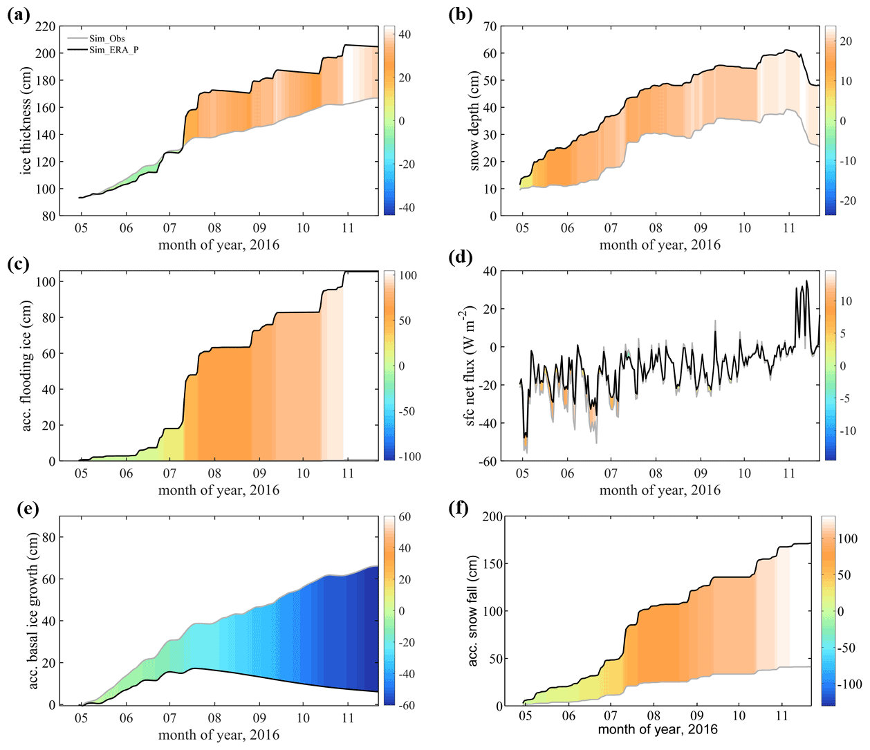
Figure 4Times series of (a) sea ice thickness, (b) snow depth, (c) accumulated flood ice, (d) net surface heat flux, (e) accumulated basal ice growth, and (f) accumulated snowfall. The gray line represents the simulation using precipitation from observations (Sim_Obs). The black line represents the simulation using precipitation from ERA5 (Sim_ERA_P). The color bar represents their difference (Sim_ERA_P − Sim_Obs).
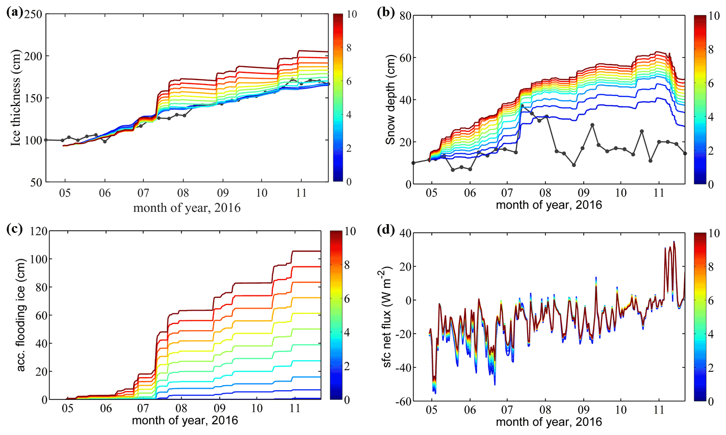
Figure 5Time series of the simulated (a) sea ice thickness, (b) snow depth, (c) accumulated flood ice, and (d) net surface heat flux in the n experiments of SEN3. The solid black point lines show the in situ observations (Obs). The 11 colored lines denote the 11 sensitivity experiments. When n=0, precipitation is from the in situ observations. When n=10, precipitation is from ERA5.
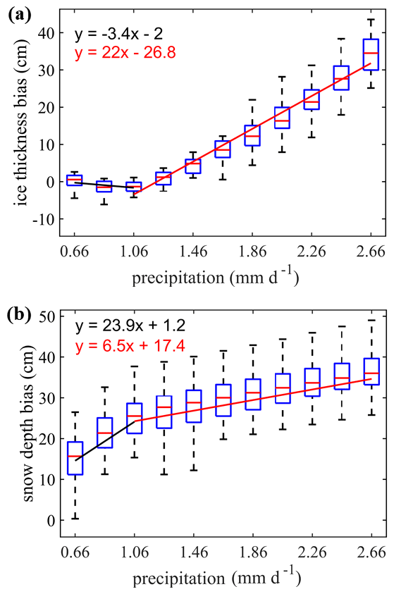
Figure 6Box plot of simulation bias (simulation minus observation) of (a) sea ice thickness and (b) snow depth over the daily mean precipitation in the different sensitivity experiments (n increases from left to right). On the x axis, 0.66 mm refers to the experiment with n=0 (in situ precipitation), and 2.66 mm refers to the n=10 experiment (ERA5 precipitation). Two linear regression lines (black and red) are derived for x≤1.06 mm and x>1.06 mm based on the mean of ice thickness and snow depth.
3.5 Additional sensitivity simulations on the precipitation bias
The precipitation from ERA5 shows the most significant deviation compared to the in situ observations and contributes the largest sea ice and snow simulation bias. To determine the cause of differences in the sea ice and snow response to precipitation, we set up 10 sensitivity experiments named SEN3 (Fig. 5). In the nth experiment, n×10 % of the daily difference between P from ERA5 and the in situ observations is added to the observed P on that day. This procedure gradually increases the magnitude of the precipitation in the experiments, while the timing of the daily precipitation events remains almost unchanged.
We define the bias as the difference between simulations and observations from 27 July to the end of November. Different start or end dates of this period do not change this result. The bias of both sea ice thickness and snow depth linearly grows with increasing precipitation (Fig. 6). The simulation bias of the sea ice thickness is relatively small before the precipitation increases by about 1 mm per day. We suggested that the snow-ice formation is small (Fig. 5c), and the insulation of the snow layer (Fig. 5d) hampers the sea ice growth. In fact, the simulated sea ice thickness even decreases (at a rate of −3.4 cm (mm d−1)−1) when the added precipitation is <1 mm d−1. When the added precipitation is >1 mm d−1, the simulated sea ice thickness quickly increases at a rate of 22 cm (mm d−1)−1.
In contrast, the simulated snow depth increases rapidly at 23.9 cm (mm d−1)−1 when the enforced precipitation remains small but at a rate of 6.5 cm when the added precipitation is large. This is because more snow is converted into flood ice, and the snow-ice formation process strongly overrules the larger insulation effect from the snow layer, promoting sea ice growth.
The snow-ice process is based on Archimedes' principle. Therefore, the threshold value (1 mm d−1) is related to the density value of ice, snow, and water in the model parameterization, as well as the sea ice thickness and snow depth. If sea ice, snow density, and initial snow depth decrease, or seawater density and initial ice thickness increase, the threshold will increase, and vice versa. These different effects of increases in precipitation on the snow and sea ice growth are illustrated in Fig. 7, emphasizing the role of flooding via snow-ice formation. When the snow layer is shallow, increases in precipitation will quickly deepen the snow layer and inhibit the growth of sea ice thickness due to the insulation of snow. The decrease in the surface net heat flux is the dominant factor. While the snow layer is deep and a lot of precipitation is present, the flooding process induces snow-ice formation, and the sea ice grows quickly, while the snow depth increases only slowly.
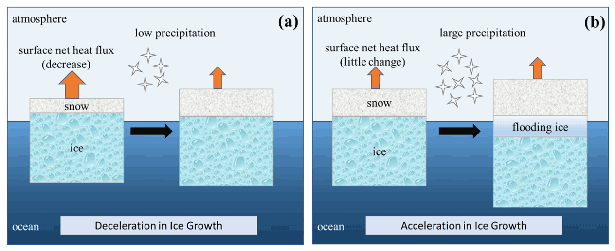
Figure 7Schematic diagram for (a) low precipitation and (b) large precipitation events illustrating the precipitation effect on sea ice growth. The orange arrows represent surface net heat flux, and different colored boxes indicate the layer of snow, flood ice, and sea ice.
The simulated ice thickness and snow depth deviate from the observations in this study (Fig. 3). We list the shortcomings that could affect the simulation: (1) superimposed ice is not considered in this study; (2) the snow-ice formation might be overestimated on the landfast sea ice in ICEPACK; and (3) the snowdrift process has not been involved in the version of ICEPACK used here.
Superimposed ice is present in early autumn when the snow starts to melt (Kawamura et al., 1997) and contributes significantly to sea ice growth (up to 20 % of mass) (Granskog et al., 2004). Superimposed ice usually corresponds to liquid precipitation or melted snow that permeates downward to form a fresh slush layer and refreezes. The superimposed ice is implemented in ICEPACK via the melt pond parametrization but has not been considered in this study. Therefore, the simulation may underestimate sea ice thickness and overestimate snow depth compared to the observations in November (Fig. 3a). We will apply the melt pond scheme in follow-up research work.
Flooding-induced snow-ice formation is common in the Antarctic Ocean because of the thin ice and heavy snowfall (Kawamura et al., 1997). It can contribute to considerable ice mass (12 %–36 %) and reduce the snow depth by up to 42 %–70 %, depending on the season and location (Jeffries et al., 2001). The parameterization of the flooding process in ICEPACK is based on Archimedes' principle for the pack ice, which might be problematic for the coastal landfast sea ice. With a much larger volume and shallower seawater around than the pack sea ice, part of the coastal landfast sea ice might contact the sea bed rather than float in the sea. Thus, the flooding should be much weaker even with weighted snow cover. Moreover, the change in density of ice due to the flooding process is significant (Saloranta, 2000) but not well considered in ICEPACK. For example, a slushy layer of 10 cm depth would refreeze within 3 d from observations (Provost et al., 2017), while the process only needs 1 d in ICEPACK. Hence, the landfast sea ice growth due to snow-ice formation needs improvement in ICEPACK, especially when the input precipitation is significantly exaggerated, e.g., the ERA5 forcing.
Surface drifting snow particles play an essential role in the surface mass balance (M. R. Van den Broeke et al., 2004). Figure 3b shows that the observed snow depth has quickly decreased from 32 cm on 2 August to 15.5 cm on 10 August, which should be attributed to the snowdrift because the surface wind is >8 m s−1 in most of this period (Fig. 2c). Friction velocity becomes sufficiently high to overcome the gravity and bonds between snow particles in this strong wind and raise the snow particles from the surface (van den Broeke et al., 2006; Thiery et al., 2012; Tanji et al., 2021). However, the mean surface wind in ERA5 is convergent around the observation site during the intense wind period (Fig. 8), which might not be expected for snow depth to decrease due to snowdrift. The coarse resolution of the atmospheric reanalysis might not produce a realistic surface wind field, which is primarily determined by the local topography (Van Den Broeke et al., 1999; Frezzotti et al., 2005). In addition, surface sublimation of drifting snow particles, which is most significant in warm, dry, and windy weather (Thiery et al., 2012), plays an important role in surface mass balance (M. R. Van den Broeke et al., 2004) but has not been involved in ICEPACK yet.
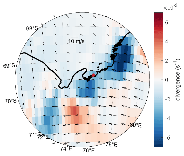
Figure 8The mean ERA5 surface wind and divergence from 2 to 10 August. The black line represents the coastline, and the red point represents the observation site.
The surface wind can affect the snow depth by changing the surface heat fluxes (Fairall et al., 2003). Compared with Sim_Obs, Sim_ERA_W gives a W m−2 lower latent heat flux (positive downward) on average (Fig. 9b), i.e., a larger sublimation (Fig. 9c), and a reduction of about −3.4 cm of the snow depth (Fig. 9a). Therefore, the overestimation in the surface wind from ERA5 partly neutralizes the effect of overestimated precipitation.
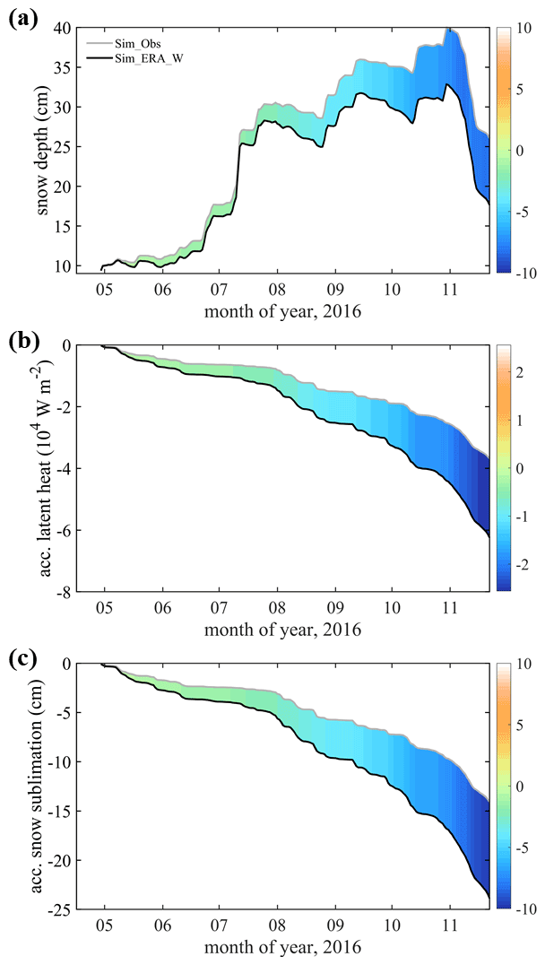
Figure 9Times series of (a) snow depth, (b) accumulated latent heat flux, and (c) accumulated snow sublimation. The gray line represents the simulation using wind from the observations (Sim_Obs). The black line represents the simulation using wind from ERA5 (Sim_ERA_W). The color bar represents their difference (Sim_ERA_W − Sim_Obs).
The oceanic forcing also plays an essential role in sea ice evolution (Uotila et al., 2019). Heat flux from the ocean boundary layer changes the sea ice energy balance (Maykut and Untersteiner, 1971). The ocean heat flux is mainly impacted by summer insolation through open leads, thin ice, melt ponds (Perovich and Maykut, 1990), and upward heat transfer through vertical turbulent mixing (McPhee et al., 1999). Because the oceanic observations under sea ice are challenging, most sea ice models directly use some empirical values, like the default value in CCSM3, to build the ocean boundary condition (e.g., Y. Yang et al., 2016; Turner and Hunke, 2015). Although some oceanic variables, like the water temperature and salinity, are from observations, others refer to previous studies, like the mixed layer depth. The uncertainty in oceanic forcing might be as important as the atmospheric ones, which will be focused on in our coming work.
This work uses the single-column sea ice model ICEPACK forced by the ERA5 atmospheric reanalysis and atmospheric in situ observations to simulate snow depth and sea ice thickness at Zhongshan Station, Antarctic. We find that forced by atmospheric variables from in situ observations, ICEPACK can reasonably simulate the sea ice thickness evolution, but it significantly overestimates the snow depth after the heavy snowfall on 11 July. When using atmospheric forcing from ERA5, sea ice thickness simulation is close to observations before 11 July but suddenly increases after the snowfall event.
From the sensitivity experiments, we find that the significant deviation in the precipitation of ERA5 contributes to the largest bias in both sea ice thickness and snow depth even though the precipitation is moderately sensitive to sea ice thickness (−0.032 cm %−1) and snow depth (0.135 cm %−1). On average, about 2 mm d−1 more precipitation in ERA5 is found during the observation period, which produces about 14.5 cm excess sea ice thickness and 17.3 cm more snow depth.
We further explore the physical mechanism of the effect of precipitation on ice thickness. Snow-ice formation can be triggered by a heavy snowfall episode, like on 11 July. It efficiently produces ice at the sea ice surface, decelerates the snow accumulation, and inhibits sea ice's basal growth. When the snowfall is weak, the snow layer thickens quickly and hampers the sea ice growth through its insulation effect. When the snowfall increases to a certain degree (∼1 mm d−1), it will trigger a continuous flooding process, accelerating the sea ice growth and slowing down the snow layer thickening.
ERA5 reanalysis atmospheric data were released by the European Centre for Medium-range Weather Forecasts (ECMWF; https://doi.org/10.24381/cds.adbb2d47, Hersbach et al., 2018). Sea ice observed data are available upon request to the corresponding author.
QY and BH conceptualized this study and designed the numerical experiments. FG carried out the numerical experiments and wrote the manuscript. BH, FK, CL, and QY helped analyze the results and revised the manuscript. GH provided and helped process the sea ice observation data. CYY, JL, PH, and XL assisted during the writing progress and critically discussed the contents.
At least one of the (co-)authors is a member of the editorial board of The Cryosphere. The peer-review process was guided by an independent editor, and the authors also have no other competing interests to declare.
Publisher's note: Copernicus Publications remains neutral with regard to jurisdictional claims in published maps and institutional affiliations.
The authors would like to thank ECMWF for the ERA5 reanalysis data set and the Russian meteorological station Progress II for the precipitation observations. We are grateful to the CICE Consortium for sharing ICEPACK and its documentation (https://github.com/CICE-Consortium/Icepack, last access: 23 October 2020).
This research has been supported by the National Natural Science Foundation of China (grant nos. 41941009, 41922044, and 42105072), the Guangdong Basic and Applied Basic Research Foundation (grant nos. 2020B1515020025 and 2021A1515012209), the Southern Marine Science and Engineering Guangdong Laboratory (Zhuhai) (grant no. SML2020SP007), and CAS “Light of West China” Program (grant nos. E129030101, Y929641001). Petra Heil was supported by AAS (grant no. 4506).
This paper was edited by David Schroeder and reviewed by three anonymous referees.
Barthélemy, A., Goosse, H., Fichefet, T., and Lecomte, O.: On the sensitivity of Antarctic sea ice model biases to atmospheric forcing uncertainties, Clim. Dynam., 51, 1585–1603, https://doi.org/10.1007/s00382-017-3972-7, 2018.
Bitz, C. M., Holland, M. M., Weaver, A. J., and Eby, M.: Simulating the ice-thickness distribution in a coupled climate model, J. Geophys. Res.-Oceans, 106, 2441–2463, https://doi.org/10.1029/1999JC000113, 2001.
Bracegirdle, T. J. and Marshall, G. J.: The reliability of Antarctic tropospheric pressure and temperature in the latest global reanalyses, J. Climate, 25, 7138–7146, https://doi.org/10.1175/JCLI-D-11-00685.1, 2012.
Briegleb, B. P. and Light, B.: A Delta-Eddington multiple scattering parameterization for solar radiation in the sea ice component of the Community Climate System Model, NCAR Tech. Note NCAR/TN-472+ STR, 1-108, https://github.com/CICE-Consortium/CICE/blob/master/doc/PDF/BL_NCAR2007.pdf (last access: 14 May 2022), 2007.
Bromwich, D. H., Fogt, R. L., Hodges, K. I., and Walsh, J. E.: A tropospheric assessment of the ERA-40, NCEP, and JRA-25 global reanalyses in the polar regions, J. Geophys. Res.-Atmos., 112, D10111, https://doi.org/10.1029/2006JD007859, 2007.
Chemke, R. and Polvani, L. M.: Using multiple large ensembles to elucidate the discrepancy between the 1979–2019 modeled and observed Antarctic sea ice trends, Geophys. Res. Lett., 47, e2020G–e88339G, https://doi.org/10.1029/2020GL088339, 2020.
Cheng, B., Zhang, Z., Vihma, T., Johansson, M., Bian, L., Li, Z., and Wu, H.: Model experiments on snow and ice thermodynamics in the Arctic Ocean with CHINARE 2003 data, J. Geophys. Res.-Oceans, 113, C9020, https://doi.org/10.1029/2007JC004654, 2008.
Cheng, B., Mäkynen, M., Similä, M., Rontu, L., and Vihma, T.: Modelling snow and ice thickness in the coastal Kara Sea, Russian Arctic, Ann. Glaciol., 54, 105–113, https://doi.org/10.3189/2013AoG62A180, 2013.
Collins, W. D., Bitz, C. M., Blackmon, M. L., Bonan, G. B., Bretherton, C. S., Carton, J. A., Chang, P., Doney, S. C., Hack, J. J., and Henderson, T. B.: The community climate system model version 3 (CCSM3), J. Climate, 19, 2122–2143, https://doi.org/10.1175/JCLI3761.1, 2006.
Fairall, C. W., Bradley, E. F., Hare, J. E., Grachev, A. A., and Edson, J. B.: Bulk parameterization of air–sea fluxes: Updates and verification for the COARE algorithm, J. Climate, 16, 571–591, https://doi.org/10.1175/1520-0442(2003)016<0571:BPOASF>2.0.CO;2, 2003.
Fréville, H., Brun, E., Picard, G., Tatarinova, N., Arnaud, L., Lanconelli, C., Reijmer, C., and van den Broeke, M.: Using MODIS land surface temperatures and the Crocus snow model to understand the warm bias of ERA-Interim reanalyses at the surface in Antarctica, The Cryosphere, 8, 1361–1373, https://doi.org/10.5194/tc-8-1361-2014, 2014.
Frezzotti, M., Pourchet, M., Flora, O., Gandolfi, S., Gay, M., Urbini, S., Vincent, C., Becagli, S., Gragnani, R., and Proposito, M.: Spatial and temporal variability of snow accumulation in East Antarctica from traverse data, J. Glaciol., 51, 113–124, https://doi.org/10.3189/172756505781829502, 2005.
Gascoin, S., Lhermitte, S., Kinnard, C., Bortels, K., and Liston, G. E.: Wind effects on snow cover in Pascua-Lama, Dry Andes of Chile, Adv. Water Resour., 55, 25–39, https://doi.org/10.1016/j.advwatres.2012.11.013, 2013.
Granskog, M. A., Leppäranta, M., Kawamura, T., Ehn, J., and Shirasawa, K.: Seasonal development of the properties and composition of landfast sea ice in the Gulf of Finland, the Baltic Sea, J. Geophys. Res.-Oceans, 109, C02020, https://doi.org/10.1029/2003JC001874, 2004.
Hao, G., Yang, Q., Zhao, J., Deng, X., Yang, Y., Duan, P., Zhang, L., Li, C., and Cui, L.: Observation and analysis of landfast ice arounding Zhongshan Station, Antarctic in 2016, Haiyang Xuebao, 9, 26–39, https://doi.org/10.3969/j.issn.0253-4193.2019.09.003, 2019.
Hao, G., Pirazzini, R., Yang, Q., Tian, Z., and Liu, C.: Spectral albedo of coastal landfast sea ice in Prydz Bay, Antarctica, J. Glaciol., 67, 1–11, https://doi.org/10.1017/jog.2020.90, 2020.
Heil, P.: Atmospheric conditions and fast ice at Davis, East Antarctica: A case study, J. Geophys. Res.-Oceans, 111, C5009, https://doi.org/10.1029/2005JC002904, 2006.
Heil, P., Allison, I., and Lytle, V. I.: Seasonal and interannual variations of the oceanic heat flux under a landfast Antarctic sea ice cover, J. Geophys. Res.-Oceans, 101, 25741–25752, https://doi.org/10.1029/96JC01921, 1996.
Hersbach, H. and Dee, D.: ERA5 reanalysis is in production, ECMWF Newsletter 147, https://www.ecmwf.int/en/newsletter/147/news/era5-reanalysis-production (last access: 29 April 2020), 2016.
Hersbach, H., Bell, B., Berrisford, P., Biavati, G., Horányi, A., Muñoz Sabater, J., Nicolas, J., Peubey, C., Radu, R., Rozum, I., Schepers, D., Simmons, A., Soci, C., Dee, D., and Thépaut, J.-N.: ERA5 hourly data on single levels from 1979 to present, Copernicus Climate Change Service (C3S) Climate Data Store (CDS) [data set], https://doi.org/10.24381/cds.adbb2d47, 2018.
Hersbach, H., Bell, B., Berrisford, P., Hirahara, S., Horányi, A., Muñoz Sabater, J., Nicolas, J., Peubey, C., Radu, R., and Schepers, D.: The ERA5 global reanalysis, Q. J. Roy. Meteor. Soc., 146, 1999–2049, https://doi.org/10.1002/qj.3803, 2020.
Hunke, E., Allard, R., Bailey, D. A., Blain, P., Craig, T., Dupont, F., DuVivier, A., Grumbine, R., Hebert, D., Holland, M., Jeffery, N., Lemieux, J., Rasmussen, T., Ribergaard, M., Roberts, A., Turner, M., and Winton, M.: CICE-Consortium/Icepack: Icepack1.1.1, Zenodo [code], https://doi.org/10.5281/zenodo.3251032, 2019.
Jakobs, C. L., Reijmer, C. H., Smeets, C. P., Trusel, L. D., Van De Berg, W. J., Van Den Broeke, M. R., and Van Wessem, J. M.: A benchmark dataset of in situ Antarctic surface melt rates and energy balance, J. Glaciol., 66, 291–302, https://doi.org/10.1017/jog.2020.6, 2020.
Jeffries, M. O., Krouse, H. R., Hurst-Cushing, B., and Maksym, T.: Snow-ice accretion and snow-cover depletion on Antarctic first-year sea-ice floes, Ann. Glaciol., 33, 51–60, https://doi.org/10.3189/172756401781818266, 2001.
Jones, R. W., Renfrew, I. A., Orr, A., Webber, B., Holland, D. M., and Lazzara, M. A.: Evaluation of four global reanalysis products using in situ observations in the Amundsen Sea Embayment, Antarctica, J. Geophys. Res.-Atmos., 121, 6240–6257, https://doi.org/10.1002/2015JD024680, 2016.
Kawamura, T., Ohshima, K. I., Takizawa, T., and Ushio, S.: Physical, structural, and isotopic characteristics and growth processes of fast sea ice in Lützow-Holm Bay, Antarctica, J. Geophys. Res.-Oceans, 102, 3345–3355, https://doi.org/10.1029/96JC03206, 1997.
Lei, R., Li, Z., Cheng, B., Zhang, Z., and Heil, P.: Annual cycle of landfast sea ice in Prydz Bay, east Antarctica, J. Geophys. Res.-Oceans, 115, C2006, https://doi.org/10.1029/2008JC005223, 2010.
Leppäranta, M.: A growth model for black ice, snow ice and snow thickness in subarctic basins, Hydrol. Res., 14, 59–70, https://doi.org/10.2166/nh.1983.0006, 1983.
Lindsay, R. and Schweiger, A.: Arctic sea ice thickness loss determined using subsurface, aircraft, and satellite observations, The Cryosphere, 9, 269–283, https://doi.org/10.5194/tc-9-269-2015, 2015.
Lindsay, R., Wensnahan, M., Schweiger, A., and Zhang, J.: Evaluation of seven different atmospheric reanalysis products in the Arctic, J. Climate, 27, 2588–2606, https://doi.org/10.1175/JCLI-D-13-00014.1, 2014.
Liston, G. E., Polashenski, C., Rösel, A., Itkin, P., King, J., Merkouriadi, I., and Haapala, J.: A distributed snow-evolution model for sea-ice applications (SnowModel), J. Geophys. Res.-Oceans, 123, 3786–3810, https://doi.org/10.1002/2017JC013706, 2018.
Liu, C., Gao, Z., Yang, Q., Han, B., Wang, H., Hao, G., Zhao, J., Yu, L., Wang, L., and Li, Y.: Measurements of turbulence transfer in the near-surface layer over the Antarctic sea-ice surface from April through November in 2016, Ann. Glaciol., 61, 12–23, https://doi.org/10.1017/aog.2019.48, 2020.
Liu, C., Hao, G., Li, Y., Zhao, J., Lei, R., Cheng, B., Gao, Z., and Yang, Q.: The sensitivity of parameterization schemes in thermodynamic modeling of the landfast sea ice in Prydz Bay, East Antarctica, J. Glaciol., 1–16, https://doi.org/10.1017/jog.2022.8, 2022.
Massom, R. A., Eicken, H., Hass, C., Jeffries, M. O., Drinkwater, M. R., Sturm, M., Worby, A. P., Wu, X., Lytle, V. I., and Ushio, S.: Snow on Antarctic sea ice, Rev. Geophys., 39, 413–445, https://doi.org/10.1029/2000RG000085, 2001.
Massonnet, F., Fichefet, T., Goosse, H., Vancoppenolle, M., Mathiot, P., and König Beatty, C.: On the influence of model physics on simulations of Arctic and Antarctic sea ice, The Cryosphere, 5, 687–699, https://doi.org/10.5194/tc-5-687-2011, 2011.
Maykut, G. A. and McPhee, M. G.: Solar heating of the Arctic mixed layer, J. Geophys. Res.-Oceans, 100, 24691–24703, https://doi.org/10.1029/95JC02554, 1995.
Maykut, G. A. and Untersteiner, N.: Some results from a time-dependent thermodynamic model of sea ice, J. Geophys. Res., 76, 1550–1575, https://doi.org/10.1029/JC076i006p01550, 1971.
McPhee, M. G., Kottmeier, C., and Morison, J. H.: Ocean Heat Flux in the Central Weddell Sea during Winter, J. Phys. Oceanogr., 29, 1166–1179, https://doi.org/10.1175/1520-0485(1999)029<1166:OHFITC>2.0.CO;2, 1999.
Merkouriadi, I., Liston, G. E., Graham, R. M., and Granskog, M. A.: Quantifying the potential for snow-ice formation in the Arctic Ocean, Geophys. Res. Lett., 47, e2019GL085020, https://doi.org/10.1029/2019GL085020, 2020.
Parkinson, C. L.: A 40-y record reveals gradual Antarctic sea ice increases followed by decreases at rates far exceeding the rates seen in the Arctic, P. Natl. Acad. Sci. USA, 116, 14414–14423, https://doi.org/10.1073/pnas.1906556116, 2019.
Parkinson, C. L. and Cavalieri, D. J.: Antarctic sea ice variability and trends, 1979–2010, The Cryosphere, 6, 871–880, https://doi.org/10.5194/tc-6-871-2012, 2012.
Perovich, D. K. and Maykut, G. A.: Solar heating of a stratified ocean in the presence of a static ice cover, J. Geophys. Res.-Oceans, 95, 18233–18245, https://doi.org/10.1029/JC095iC10p18233, 1990.
Powell, D. C., Markus, T., and Stössel, A.: Effects of snow depth forcing on Southern Ocean sea ice simulations, J. Geophys. Res.-Oceans, 110, C6001, https://doi.org/10.1029/2003JC002212, 2005.
Provost, C., Sennéchael, N., Miguet, J., Itkin, P., Rösel, A., Koenig, Z., Villacieros Robineau, N., and Granskog, M. A.: Observations of flooding and snow-ice formation in a thinner Arctic sea-ice regime during the N-ICE2015 campaign: Influence of basal ice melt and storms, J. Geophys. Res.-Oceans, 122, 7115–7134, https://doi.org/10.1002/2016JC012011, 2017.
Roussel, M.-L., Lemonnier, F., Genthon, C., and Krinner, G.: Brief communication: Evaluating Antarctic precipitation in ERA5 and CMIP6 against CloudSat observations, The Cryosphere, 14, 2715–2727, https://doi.org/10.5194/tc-14-2715-2020, 2020.
Saloranta, T. M.: Modeling the evolution of snow, snow ice and ice in the Baltic Sea, Tellus A, 52, 93–108, https://doi.org/10.3402/tellusa.v52i1.12255, 2000.
Schlosser, E., Haumann, F. A., and Raphael, M. N.: Atmospheric influences on the anomalous 2016 Antarctic sea ice decay, The Cryosphere, 12, 1103–1119, https://doi.org/10.5194/tc-12-1103-2018, 2018.
Stroeve, J. C., Serreze, M. C., Holland, M. M., Kay, J. E., Malanik, J., and Barrett, A. P.: The Arctic's rapidly shrinking sea ice cover: a research synthesis, Clim. Change, 110, 1005–1027, https://doi.org/10.1007/s10584-011-0101-1, 2012.
Stuecker, M. F., Bitz, C. M., and Armour, K. C.: Conditions leading to the unprecedented low Antarctic sea ice extent during the 2016 austral spring season, Geophys. Res. Lett., 44, 9008–9019, https://doi.org/10.1002/2017GL074691, 2017.
Tanji, S., Inatsu, M., and Okaze, T.: Development of a snowdrift model with the lattice Boltzmann method, Prog. Earth Planet. Sci., 8, 1–16, https://doi.org/10.1186/s40645-021-00449-0, 2021.
Tetzner, D., Thomas, E., and Allen, C.: A Validation of ERA5 Reanalysis Data in the Southern Antarctic Peninsula–Ellsworth Land Region, and Its Implications for Ice Core Studies, Geosciences, 9, 289, https://doi.org/10.3390/geosciences9070289, 2019.
Thiery, W., Gorodetskaya, I. V., Bintanja, R., Van Lipzig, N. P. M., Van den Broeke, M. R., Reijmer, C. H., and Kuipers Munneke, P.: Surface and snowdrift sublimation at Princess Elisabeth station, East Antarctica, The Cryosphere, 6, 841–857, https://doi.org/10.5194/tc-6-841-2012, 2012.
Tsamados, M., Feltham, D. L., and Wilchinsky, A. V.: Impact of a new anisotropic rheology on simulations of Arctic sea ice, J. Geophys. Res.-Oceans, 118, 91–107, https://doi.org/10.1029/2012JC007990, 2013.
Turner, A. K. and Hunke, E. C.: Impacts of a mushy-layer thermodynamic approach in global sea-ice simulations using the CICE sea-ice model, J. Geophys. Res.-Oceans, 120, 1253–1275, https://doi.org/10.1002/2014JC010358, 2015.
Turner, A. K., Hunke, E. C., and Bitz, C. M.: Two modes of sea-ice gravity drainage: A parameterization for large-scale modeling, J. Geophys. Res.-Oceans, 118, 2279–2294, https://doi.org/10.1002/jgrc.20171, 2013.
Turner, J., Phillips, T., Marshall, G. J., Hosking, J. S., Pope, J. O., Bracegirdle, T. J., and Deb, P.: Unprecedented springtime retreat of Antarctic sea ice in 2016, Geophys. Res. Lett., 44, 6868–6875, https://doi.org/10.1002/2017GL073656, 2017.
Uotila, P., Goosse, H., Haines, K., Chevallier, M., Barthélemy, A., Bricaud, C., Carton, J., Fučkar, N., Garric, G., and Iovino, D.: An assessment of ten ocean reanalyses in the polar regions, Clim. Dynam., 52, 1613–1650, https://doi.org/10.1007/s00382-018-4242-z, 2019.
Urraca, R., Huld, T., Gracia-Amillo, A., Martinez-de-Pison, F. J., Kaspar, F., and Sanz-Garcia, A.: Evaluation of global horizontal irradiance estimates from ERA5 and COSMO-REA6 reanalyses using ground and satellite-based data, Sol. Energy, 164, 339–354, https://doi.org/10.1016/j.solener.2018.02.059, 2018.
Vancoppenolle, M., Timmermann, R., Ackley, S. F., Fichefet, T., Goosse, H., Heil, P., Leonard, K. C., Lieser, J., Nicolaus, M., and Papakyriakou, T.: Assessment of radiation forcing data sets for large-scale sea ice models in the Southern Ocean, Deep-Sea Res., Pt. II, 58, 1237–1249, https://doi.org/10.1016/j.dsr2.2010.10.039, 2011.
Van Den Broeke, M. R., Winther, J., Isaksson, E., Pinglot, J. F., Karlöf, L., Eiken, T., and Conrads, L.: Climate variables along a traverse line in Dronning Maud Land, East Antarctica, J. Glaciol., 45, 295–302, https://doi.org/10.3189/S0022143000001799, 1999.
Van Den Broeke, M., Reijmer, C., and Van De Wal, R.: Surface radiation balance in Antarctica as measured with automatic weather stations, J. Geophys. Res.-Atmos., 109, D09103, https://doi.org/10.1029/2003JD004394, 2004.
van den Broeke, M., van de Berg, W. J., van Meijgaard, E., and Reijmer, C.: Identification of Antarctic ablation areas using a regional atmospheric climate model, J. Geophys. Res.-Atmos, 111, D18110, https://doi.org/10.1029/2006JD007127, 2006.
Van Den Broeke, M. R., Reijmer, C. H., and Van De Wal, R. S.: A study of the surface mass balance in Dronning Maud Land, Antarctica, using automatic weather stations, J. Glaciol., 50, 565–582, https://doi.org/10.3189/172756504781829756, 2004.
Vignon, é., Traullé, O., and Berne, A.: On the fine vertical structure of the low troposphere over the coastal margins of East Antarctica, Atmos. Chem. Phys., 19, 4659–4683, https://doi.org/10.5194/acp-19-4659-2019, 2019.
Wang, C., Cheng, B., Wang, K., Gerland, S., and Pavlova, O.: Modelling snow ice and superimposed ice on landfast sea ice in Kongsfjorden, Svalbard, Polar Res., 34, 20828, https://doi.org/10.3402/polar.v34.20828, 2015.
Wang, C., Graham, R. M., Wang, K., Gerland, S., and Granskog, M. A.: Comparison of ERA5 and ERA-Interim near-surface air temperature, snowfall and precipitation over Arctic sea ice: effects on sea ice thermodynamics and evolution, The Cryosphere, 13, 1661–1679, https://doi.org/10.5194/tc-13-1661-2019, 2019.
Wang, G., Hendon, H. H., Arblaster, J. M., Lim, E., Abhik, S., and van Rensch, P.: Compounding tropical and stratospheric forcing of the record low Antarctic sea-ice in 2016, Nat. Commun., 10, 1–9, https://doi.org/10.1038/s41467-018-07689-7, 2019.
Wang, Y., Zhou, D., Bunde, A., and Havlin, S.: Testing reanalysis data sets in Antarctica: Trends, persistence properties, and trend significance, J. Geophys. Res.-Atmos., 121, 12–839, https://doi.org/10.1002/2016JD024864, 2016.
Yang, Q., Liu, J., Leppäranta, M., Sun, Q., Li, R., Zhang, L., Jung, T., Lei, R., Zhang, Z., and Li, M.: Albedo of coastal landfast sea ice in Prydz Bay, Antarctica: Observations and parameterization, Adv. Atmos. Sci., 33, 535–543, https://doi.org/10.1007/s00376-015-5114-7, 2016a.
Yang, Y., Zhijun, L., Leppäranta, M., Cheng, B., Shi, L., and Lei, R.: Modelling the thickness of landfast sea ice in Prydz Bay, East Antarctica, Antarct. Sci., 28, 59–70, https://doi.org/10.1017/S0954102015000449, 2016b.
Zhang, J.: Increasing Antarctic sea ice under warming atmospheric and oceanic conditions, J. Climate, 20, 2515–2529, https://doi.org/10.1175/JCLI4136.1, 2007.
Zhang, J.: Modeling the impact of wind intensification on Antarctic sea ice volume, J. Climate, 27, 202–214, https://doi.org/10.1175/JCLI-D-12-00139.1, 2014.
Zhao, J., Cheng, B., Yang, Q., Vihma, T., and Zhang, L.: Observations and modelling of first-year ice growth and simultaneous second-year ice ablation in the Prydz Bay, East Antarctica, Ann. Glaciol., 58, 59–67, https://doi.org/10.1017/aog.2017.33, 2017.
Zhao, J., Cheng, B., Vihma, T., Yang, Q., Hui, F., Zhao, B., Hao, G., Shen, H., and Zhang, L.: Observation and thermodynamic modeling of the influence of snow cover on landfast sea ice thickness in Prydz Bay, East Antarctica, Cold Reg. Sci. Technol., 168, 102869, https://doi.org/10.1016/j.coldregions.2019.102869, 2019.