the Creative Commons Attribution 4.0 License.
the Creative Commons Attribution 4.0 License.
 | 13 May 2022
Kara and Barents sea ice thickness estimation based on CryoSat-2 radar altimeter and Sentinel-1 dual-polarized synthetic aperture radar
Juha Karvonen
Eero Rinne
Heidi Sallila
Petteri Uotila
Marko Mäkynen
We present a method to combine CryoSat-2 (CS2) radar altimeter and Sentinel-1 synthetic aperture radar (SAR) data to obtain sea ice thickness (SIT) estimates for the Barents and Kara seas. From the viewpoint of tactical navigation, along-track altimeter SIT estimates are sparse, and the goal of our study is to develop a method to interpolate altimeter SIT measurements between CS2 ground tracks. The SIT estimation method developed here is based on the interpolation of CS2 SIT utilizing SAR segmentation and segmentwise SAR texture features. The SIT results are compared to SIT data derived from the AARI ice charts; to ORAS5, PIOMAS and TOPAZ4 ocean–sea ice data assimilation system reanalyses; to combined CS2 and Soil Moisture and Ocean Salinity (SMOS) radiometer weekly SIT (CS2SMOS SIT) charts; and to the daily MODIS (Moderate Resolution Imaging Spectroradiometer) SIT chart. We studied two approaches: CS2 directly interpolated to SAR segments and CS2 SIT interpolated to SAR segments with mapping of the CS2 SIT distributions to correspond to SIT distribution of the PIOMAS ice model. Our approaches yield larger spatial coverage and better accuracy compared to SIT estimates based on either CS2 or SAR data alone. The agreement with modelled SIT is better than with the CS2SMOS SIT. The average differences when compared to ice models and the AARI ice chart SIT were typically tens of centimetres, and there was a significant positive bias when compared to the AARI SIT (on average 27 cm) and a similar bias (24 cm) when compared to the CS2SMOS SIT. Our results are directly applicable to the future CRISTAL mission and Copernicus programme SAR missions.
- Article
(4083 KB) - Full-text XML
- BibTeX
- EndNote


The goal of this study is to use Sentinel-1 (S-1) C-band SAR data to interpolate CryoSat-2 (CS2) sea ice thickness (SIT) estimates to spatially cover the whole Barents Sea and Kara Sea (BKS) area (see Fig. 1). We have chosen this study area because we have collected S-1 data over BKS since 2015 and also generated daily S-1 mosaics covering the area. Using a combination of the CS2 and S-1 data, it is possible to estimate SIT with much finer resolution and much larger spatial coverage than using only the CS2, or another altimeter data. The interpolated CS2 SIT is assigned for classified SAR segments, i.e. locally uniform sea ice areas in the SAR imagery. In this way we are able to provide accurate boundaries of different ice areas and provide a typical SIT for each of these areas based on the CS2 SIT data conducted within the areas themselves or nearby similar areas.
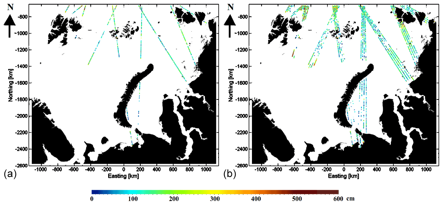
Figure 1CryoSat-2 sea ice thickness measurements during 1 d (a) and 1 week (b) before 21 February 2017.
SIT is one of the essential climate variables. It is a key parameter, together with sea ice concentration (SIC), for estimating total ice volume over any given area of interest. Accurate estimates of SIT are important for ice navigation, off-shore engineering and construction (IMarEST, 2015), climate studies, and sea ice and weather forecasting (Jung et al., 2014). The ocean–atmosphere heat, mass, momentum and gas exchanges are controlled by the SIT distribution in the polar oceans. Thin ice with a thickness of less than half a metre produces strong heat and salt fluxes and affects the weather and deep water circulation in the polar oceans (McPhee, 2008). Thick ice insulates the relatively warm ocean from the cold atmosphere maintaining the polar conditions and is mainly responsible for the proportion of ice that persists through the summer melt period, which is particularly important for the summer radiation budget.
Estimation of SIT with SAR data has been studied before. In the Baltic Sea, SIT estimation of deformed ice under dry snow conditions is possible through a statistical relationship between the ice freeboard and the radar backscatter (Simila et al., 2010). The standard deviation of the average large-scale surface roughness increases with increasing average surface roughness, and, as the average surface roughness increases, the backscatter also increases. In Simila et al. (2010) an exponential empirical model was derived for estimating average surface roughness from the backscattering coefficient (σ0) and dominant thickness of level ice. A good correlation between the L- and C-band co-polarization ratio and SIT of undeformed ice in the Sea of Okhotsk has been found (Nakamura et al., 2006). The co-polarization ratio has little sensitivity to ice surface roughness and is related to variations in salinity, i.e. ice surface dielectric constant, that can be caused by changes in SIT (Wakabayashi et al., 2004). Toyota et al. (2011) found good correlation between ALOS/PALSAR L-band HH-polarization σ0 and SIT (R = 0.86) and surface roughness (R = 0.70) in the seasonal ice zone (SIZ) and derived linear relation between σ0 and SIT (SIT from 0.2 to 0.6 m). They suggested that satellite L-band σ0 data allow the estimation of SIT distribution in the SIZ, where surface roughness is closely related with the SIT distribution through deformation processes. Airborne C-band polarimetric SAR (POLSAR) data together with a theoretical backscattering model have been used to estimate SIT in the 0–10 cm range (Kwok et al., 1995). Zhang et al. (2016) derived a SIT estimation method for undeformed first-year ice under dry snow conditions based on a sea ice thermodynamic model and forward scattering model for C-band compact polarimetric (CP) SAR images. Using simulated CP imagery from RADARSAT-2 POLSAR, SIT estimation was possible up to 80 cm thickness. SAR data have also been used to estimate SIT of pancake ice from the way in which the pancake ice changes the dispersion relation of the waves, dampens the wave amplitude and causes dissipation of the energy of the waves; i.e. it changes the wavelength of ocean waves as they enter the ice (Wadhams et al., 2018). SIT retrieval methods based only on the SAR data are still experimental, and no operational solutions are yet available.
As indicated by these earlier studies, SAR, especially C-band SAR (S-1), alone is not capable of accurately estimating Arctic SIT. Thus, complementary data are required for reasonable Arctic SIT estimation. In this paper we try to overcome this deficiency by proposing a method to utilize CS2 SIT as complementary data to SAR data to estimate Arctic SIT.
Detection of thin ice and its thickness estimation can be done using satellite thermal infrared (TIR) imagery, e.g. from Moderate Resolution Imaging Spectroradiometer (MODIS). Satellite-based ice surface temperature (Ts) is combined with atmospheric forcing data through the ice surface heat balance equation for the SIT estimation (Yu and Rothrock, 2016). Unfortunately, this method is restricted by cloud cover and quality of cloud masking in polar conditions (Frey at al., 2008). A daily MODIS SIT chart combined from swath SIT charts, which mitigates the cloud problem, has been developed in Makynen and Karvonen (2017a). In addition, daily cloud-cover-corrected MODIS SIT composites for polynya monitoring in the Arctic and Antarctic have been produced utilizing several days of swath data (Paul et al., 2015; Preußer et al., 2016).
Thin-ice detection and its SIT estimation in winter conditions are also possible with microwave radiometer data. Thin-ice thickness retrieval algorithms have been developed for low-frequency L-band brightness temperature (TB) data from SMOS and Soil Moisture Active Passive (SMAP) missions (Kaleschke et al., 2012; Tian-Kunze et al., 2014; Huntemann et al., 2014; Kaleschke et al., 2016; Schmitt and Kaleschke, 2018). With the SMOS data SIT can be estimated for up to 0.5–1.5 m thick ice (Kaleschke et al., 2016). The drawback of the SMOS data is their poor spatial resolution, 35–50 km, which does not allow the detection of leads and smaller polynyas. For high-frequency radiometer data (36 and 90 GHz), thin-ice SIT retrieval algorithms have also been developed (e.g. Martin et al., 2004; Iwamoto et al., 2014; Nakata et al., 2019). The thin-ice SIT can be typically estimated up to 20 cm, and the SIT data are used for polynya monitoring (e.g. Onshima et al., 2016).
Estimation of ice thickness from radar and laser altimeter data has been studied extensively in recent years. Altimeters on board several satellites have provided estimates of sea ice thickness and volume time series and trends for the Arctic and Antarctic oceans for recent decades. Such methods have been applied and evaluated in Laxon et al. (2003), Giles et al. (2008), Kwok and Cunningham (2008), Kwok et al. (2009), Armitage et al. (2015), Zygmuntowska et al. (2014), Tilling et al. (2015, 2018), Xia and Xie (2018), Yi et al. (2018), Xu et al. (2020), and Petty et al. (2020), for example. Traditionally satellite altimeters, including CS2, cannot estimate thickness of thin ice (< 0.5 m) with reasonable certainty (Wingham et al., 2006). However, the recently launched ICESat-2 improves thin-ice estimation, giving reasonable uncertainties down to SIT of approximately 0.2 m (Petty et al., 2020).
In this study we use the CS2 radar altimeter SIT data (Wingham et al., 2006). Due to the nature of altimeter measurements and the orbit pattern of the platform, CS2 gives spatially and temporally sparse SIT information on temporal scales from 1 d to a few weeks. Examples of all available CS2 ice thickness estimates during the period of 1 d and 1 week over our Barents Sea and Kara Sea study area are shown in Fig. 1. Especially for tactical navigation, these estimates are sparse. Thus, our goal is to develop a method to interpolate altimeter SIT estimates between CS2 ground tracks.
SIT estimation algorithms combining CS2 and other sources of information, e.g. the SMOS (Soil Moisture and Ocean Salinity) mission with the MIRAS (Microwave Imaging Radiometer using Aperture Synthesis) instrument, exist (Ricker et al., 2017). However, these algorithms still have relatively poor spatial and temporal resolution (25 km, weekly estimates updated daily). Therefore, algorithms fusing CS2 data with data from instruments with higher spatial and temporal resolution are needed for timely high-resolution SIT estimates. Such SIT estimates can then be used in navigation and data assimilation to high-resolution ocean–sea ice forecast models.
The structure of this paper is as follows: the study area, time period and weather conditions are described in Sect. 2. Then the data sets used in the study are described in Sect. 3, followed by the description of the data preprocessing and the proposed SIT estimation method combining CS2 SIT and SAR data in Sect. 4. The proposed SIT interpolation is based on pairwise similarity of segments and their pairwise distance and time difference. The texture similarity is measured by similarity of several segmentwise SAR texture features. The texture features and the similarity criteria are described in detail in Sect. 4. The estimation results and their evaluation are presented in Sect. 5. For evaluation we have used sea ice model data and ice chart data and also included comparisons to the SIT charts based on CS2 and the ESA SMOS radiometer data (Ricker et al., 2017) and to the MODS SIT charts (Makynen and Karvonen, 2017a). Finally, discussion and conclusions are provided in Sect. 6.
Our study covers the Kara and Barents seas; see Fig. 2. Seasonal sea ice is found over most of our study area. In the far north, however, multi-year ice (MYI) is present year-round (Johannessen et al., 2007). The average dates for the ice formation over the area vary from 10 September in the north to mid-November in the southern Kara Sea and southeastern Barents Sea (Pechora Sea) and March–April in the central Barents Sea (west of Novaya Zemlya) (Johannessen et al., 2007). Melting season begins in late April in the marginal ice zone of the Barents Sea. By the end of June the central Barents Sea and the Pechora Sea are usually ice-free. In August the ice edge reaches Svalbard and Franz Josef Land. In the Kara Sea, melting gradually begins in May and continues through July and August. Most of the Kara Sea is ice-free between mid-July and mid-August. In the Kara Sea, the ice season lasts for 6–9 months depending on the location and seasonal conditions. We have only used wintertime data (January–April, October–December) for two calendar years, 2016 and 2017. Currently, radar altimeter SIT retrieval is only possible in dry snow winter conditions (Kern et al., 2020). During the melt season the radar wave penetration in snow pack is ambiguous and surface type classification often fails due to melt ponds which give similar radar waveforms as the leads.
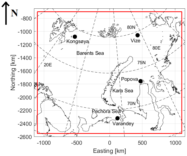
Figure 2The Barents Sea and Kara Sea study area in the used polar stereographic projection. Air temperature data from four coastal weather stations shown with black dots are used in this study. © FMI.
Throughout our study we use the coordinate system (CS) based on polar stereographic projection with a centre longitude of 55∘ E, reference latitude (latitude of the correct scale) of 70∘ N and the WGS84 datum. The upper left (UL) and lower right (LR) coordinates, i.e. the polar stereographic CS northing and easting in metres, are UL = (−700 000, −1 100 000) and LR = (−2 550 000, 1 100 000). The size of the study area is 2200 km (easting) by 1850 km (northing).
Average daily air temperature data (Ta) from four coastal weather stations (Kongsøya, Vize, Im. M.V. Popova and Varandey) shown in Fig. 2 are used to evaluate the weather conditions and periods of cold and warm weather, during our study period: January–April and October–December in 2016 and 2017. The (Ta) data from the four stations are shown in Fig. 3. Here we set ∘C to represent dry snow cold conditions, and Ta>0 ∘C for moist/wet snow conditions when the snowpack, if it exists, prevents or significantly attenuates radar returns from sea ice. Between these Ta limits, the state of the snowpack is ambiguous as it depends on Ta history and time of the CS2 and S-1 data acquisition, e.g. early morning vs. late afternoon. The Ta data will not be used to classify the CS2 and S-1 into different weather condition classes, but to support analysis on the accuracy of SIT from the combined CS2 and S-1 data. It is noted that the Ta limits above are only approximations.
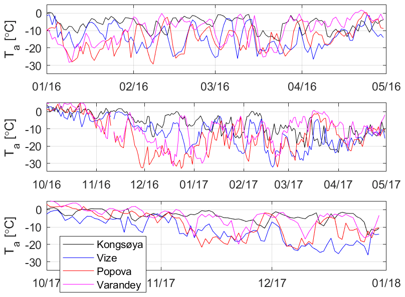
Figure 3Average daily air temperature during the period 2016–2017 from four coastal weather stations shown in Fig. 1.
During first part of our 2-year study period, from January to April 2016, our analysis of the (Ta) data from the four weather stations suggests that this time period represents typically cold dry snow conditions in our study area. The second part of the study period, from October 2016 to April 2017, covers one winter sea ice season. Our analysis shows the CS2 and S-1 data from the beginning of October to roughly mid-November are typically affected by wet or moist snow conditions, depending on the diurnal acquisition time and location in our study area (more probable in the Barents and Pechora seas). Data acquired from mid-November 2016 to April 2017 mostly represent cold winter conditions. The third, and the last, part of the study period is from October to December 2017 and represents sea ice freeze-up and early winter conditions. It seems that in the Kara Sea the time period after the first week of November 2017 can be assumed to represent mostly cold winter conditions. In the Barents and Pechora seas in November and December there are also periods of cold winter conditions, but sometimes Ta is between −5 and 0 ∘C, when there could have been moist snow effects on the radar signatures.
In this section we present the data sets used in our study.
3.1 CryoSat-2 data
CS2’s primary payload is the Synthetic Aperture Interferometric Radar Altimeter operating in the Ku-band (13.6 GHz), which allows a much smaller sampling footprint (about 300 m in the satellite along-track direction; Scagliola, 2013) than traditional pulse-limited altimeters. Over sea ice, CS2 echoes are assumed to scatter from the interface between the ice surface and the layer of overlying snow (Laxon et al., 2013), thus enabling freeboard, denoted by F here, estimation, and further SIT calculation assuming known snow depth and density and sea ice density (e.g. climatologically derived).
The quantity altimeters measure is surface elevation, from which freeboard can be derived. Assuming hydrostatic equilibrium and known sea ice density (ρi), snow density (ρs) and thickness (hs), and water density (ρw) the following equation can be formed for the SIT (hi) estimation:
In dry snow conditions, the radar scattering and backscattering penetrate the snow cover, and the backscattering comes from the ice surface; i.e. the ice freeboard is measured by a radar altimeter. In dry snow conditions hi can be estimated from the ice freeboard Fi:
As can be seen from equations above, the hs estimate has a large effect on retrieved SIT. In the case of radar altimeters, such as CS2 used here, hs is also required for wave propagation speed correction in deriving F. A more detailed analysis on the effect of snow can be found in Kern et al. (2015). In this study, like in many other CS2-based sea ice thickness products, climatological snow depth and density based on the Warren climatology (Warren et al., 1999) are used.
In this study we have computed SIT with FMI implementation of the Python sea ice radar altimetry toolbox (pysiral available in https://github.com/shendric/pysiral, last access: 10 May 2022). The primary input has been the European Space Agency's CS2 Baseline-D Level-1B product. The processing follows the algorithm of Ricker et al. (2014) and Hendricks et al. (2021a). For auxiliary data we have used the DTU15 mean sea surface height product, EUMETSAT OSISAF sea ice concentration and sea ice type, and Warren et al. (1999) snow depth and density data with the 50 % reduction over first-year ice first proposed by Kurtz and Farrell (2011).
3.2 Sentinel-1 SAR
All the available Copernicus S-1 C-band dual-polarized extra wide (EW) swath mode level 1 ground-range-detected medium-resolution (GRDM) SAR data with the HH–HV polarization channels over the BKS study area and period (January–April and October–December 2016 and January–April and October–December 2017) were used in this study. The S-1 SAR data are publicly available through the European Space Agency (ESA) Copernicus Science Hub (https://scihub.copernicus.eu/, last access: 10 May 2022). The S-1 EW SAR images cover a region of 410 km by 400 km in size, with a pixel size of 40 m and a spatial resolution of 95–91 m by 90 m (range by azimuth), and they have θ0 variation from 19 to 47∘.
3.3 Reference data
In our study we use the Russian Arctic–Antarctic Research Institute (AARI) ice charts, Ocean Reanalysis System 5 (ORAS5), Pan-Arctic Ice-Ocean Modeling and Assimilation System (PIOMAS), and TOPAZ4 ice model ocean–sea ice reanalyses SIT data, CS2SMOS SIT data (Ricker et al., 2017), and MODIS daily SIT charts (Makynen and Karvonen, 2017a) as reference data. They are used to evaluate the performance of our CS2-SAR SIT estimation method. The TOPAZ4 SIT model data are also used to remap the CryoSat-2 training data set based on cumulative SIT distributions.
3.3.1 AARI ice charts
The Arctic and Antarctic Research Institute (AARI) produces weekly ice charts for many Arctic regions, including the Barents and Kara seas (AARI, 2018; Afanasyeva et al., 2019). These charts are currently widely used for a variety of scientific and practical tasks. The main input data for the ice chart generation is remote sensing data from various optical, thermal infrared and microwave satellite sensors, including MODIS, AVHRR (Advanced Very-High-Resolution Radiometer), S-1 SAR and Sentinel-3 OLCI (Ocean and Land Colour Instrument). The regional ice charts are based on satellite imagery collected over a period of 2–3 d. The more recent information has priority. In the case of absence of up-to-date information, the data for the previous day are used. The ice charts are generated by skilled ice experts using an ArcGIS workstation. The ice analyst defines homogeneous sea ice zones, polygons on georeferenced satellite imagery, and assigns various sea ice attributes, e.g. sea ice concentration, to the polygons. In this process auxiliary data, e.g. operational monitoring of sea ice drift using satellite data and observations from hydrometeorological stations of Roshydromet, are also utilized. The main purpose of a regional weekly ice chart is to show the spatial distribution and characteristics of sea ice. The AARI weekly ice charts are in the digital SIGRID-3 vector file format (JCOMM Expert Team on Sea Ice, 2014b). The AARI ice charts are available at http://wdc.aari.ru/datasets/d0004/ (last access: 10 May 2022).
The ice charts convey their information in codes that are explained in JCOMM Expert Team on Sea Ice (2014a). The charts show total concentration (code CT) and partial concentrations of the first, second and third thickest ice (codes CA, CB and CC) along with their respective stages of development (SA, SB and SC) and form of ice (FA, FB, FC) for polygonal areas of variable sizes. The concentrations are shown with intervals of either 110 or 210 wide. The stage of development is defined as ice thickness intervals. Following thickness ranges are used: nilas (< 10 cm), young ice (10–30 cm), grey ice (10–15 cm), grey-white ice (15–30 cm), thin first-year ice (FYI) (30–70 cm), medium FYI (70–120 cm), thick FYI (≧ 120 cm), FYI in general (≧ 30 cm) and old ice (≧ 120 cm). The form of ice carries information on ice floe size or occurrence of landfast ice, for example. Some polygons only have one or two stage of development classes assigned to them (i.e. polygons are more homogeneous).
In the stage of development, i.e. SIT range, estimation of fast ice thickness measured at a hydrometeorological station serves as a reference (Afanasyeva et al., 2019). Looking at a satellite image, the ice expert matches brightness of drifting ice outside the shore to brightness of landfast ice with known thickness. Further, monitoring SIT at a seashore station allows the estimation of the rate of ice growth in remote areas. Here we interpret the AARI SIT as the thickness of level ice in the area – analogous to the thermodynamically grown fast ice.
For validation, polygons from the AARI ice charts were interpolated to a 1 km by 1 km grid covering our study area. Then for each AARI ice chart polygon a mid-range SIC and mid-range SIT or upper or lower SIT values of the first, second, and third thickest ice types were assigned. However, for FYI general type (SIT ≧ 30 cm), a SIT value of 95 cm is used (same as for thick FYI). An average SIT for each chart polygon was calculated as a sum of the SIT values for the three ice types weighted with their concentrations. Finally, the gridded charts for the Barents and Kara seas were combined; see an example in Fig. 8c. This processing of the AARI charts has been used previously by Makynen and Karvonen (2017a). The total number of the AARI weekly charts used in the validation was 37 (time span from 4 January until 26 December, excluding the summer period) for both the Barents and Kara seas.
3.3.2 CS2SMOS weekly SIT chart
The SMOS L-band brightness temperature data are currently used estimate SIT for thin-ice areas (< 1 m) (Kaleschke et al., 2012), while CS2 data allow the estimation of SIT for thicker ice (> 1 m) (Ricker et al., 2017). The CS2SMOS SIT product merges the SMOS and CS2 SIT data, which are complementary to each other. The CS2 SIT used in the merging is a weekly averaged product, and the daily SMOS SIT product is likewise averaged to a weekly temporal scale. Optimal interpolation similar to Böhme and Send (2005) and McIntosh (1990) is used to merge the data sets into the regular product grid.
3.3.3 Model reanalysis data
TOPAZ4
TOPAZ4 is a coupled ocean–sea ice model with an advanced data assimilation system for the North Atlantic Ocean and Arctic (Sakov et al., 2012). The data assimilation is based on the use of an ensemble Kalman filter (Evensen, 1994). The resolution of the TOPAZ4 model grid is 12–16 km. TOPAZ4 is operationally available in CMEMS (Copernicus Marine Environment Monitoring Service) funded by the European Commission. In this study we have used the TOPAZ4 daily reanalysis ice thickness values (CMEMS product ARCTIC_REANALYSIS_PHY_002_003) (Hackett et al., 2020). The CS2SMOS thickness (Ricker et al., 2017), based on fusion of CS2 and SMOS SIT, is assimilated to the TOPAZ4 reanalysis SIT product during wintertime, from end of October to early April. The modelled sea ice thickness provided by the TOPAZ4 CMEMS product is a diagnostic variable based on prognostically calculated sea ice volume divided by sea ice concentration for each model grid cell. Accordingly, it provides the mean sea ice thickness for the portion of grid cell that is covered by sea ice.
ORAS5
As TOPAZ4 seems to underestimate the Arctic ice thickness (Xie et al., 2018), we also used the ORAS5 (Ocean Reanalysis System 5) reanalysis SIT data (Zuo et al., 2017, 2019). Tietsche et al. (2017) calculated the root-mean-square difference between ORAS5, the prototype of ORAS5 and ICESat sea ice thicknesses to be 1.0 m, comparable to the PIOMAS product (Schweiger et al., 2011); see also Sect. 3.3.6. The ORAS5 data are produced by the European Centre for Medium-Range Weather Forecasts (ECMWF) in 0.25∘ nominal resolution in a stretched global tri-polar grid with the poles in northern Canada, Eurasia and the South Pole. This grid has a resolution of about 5–15 km in the Arctic. A feature of ORAS5 is that in the open-water part of a grid cell sea ice forms at a certain initial thickness of the order of H0=0.5 m (Tietsche et al., 2017). Such a treatment of initial sea ice is common in geophysical sea ice models (Lemieux et al., 2018). The initial thickness H0 is, coincidentally, close to the thinnest ice CS2 is able to reliably measure. Like TOPAZ4, the ORAS5 product provides the diagnostic sea ice thickness for each grid cell that has been calculated by dividing the modelled sea ice volume by concentration.
PIOMAS
Additionally we utilized the PIOMAS model (Pan-Arctic Ice Ocean Modeling and Assimilation System) (Zhang and Rothrock, 2003) SIT data, which have a coarser resolution than TOPAZ4 and ORAS5. Despite the coarse resolution, PIOMAS sea ice volume agrees well with the ICESat estimates (Schweiger et al., 2011). The PIOMAS model grid is a stretched generalized orthogonal curvilinear coordinate (GOCC) system. A GOCC system allows a coordinate transformation that displaces the pole of the model grid. The PIOMAS model data are in the GOCC grid with the northern grid pole displaced into Greenland. The PIOMAS resolution in our study area is around 40 km. Unlike TOPAZ4 and ORAS5, PIOMAS provides sea ice volume per unit area, which was divided by the PIOMAS sea ice concentration to obtain sea ice thickness per grid cell. Because of the coarse resolution of the PIOMAS data, we did not use it in direct comparisons, but we utilize it in defining the mapping of CS2 thicknesses to model-compliant thicknesses in Sect. 3.
3.3.4 MODIS daily SIT chart
Daily MODIS ice thickness (hiM) charts for our study area have been processed for two winters, from November 2015 to April 2017. All the details on the daily chart processing can be found in Makynen and Karvonen (2017a). The daily charts are based on all available Aqua and Terra MODIS hiM swath charts. Charts for very cloudy days were manually excluded. The total number of the daily charts is 317.
The MODIS-based SIT charts have a pixel size of 1 km, but the cloud mask has a 10 km pixel size. The daily hiM chart shows daily median hiM () for pixels which had at least two hiM samples from the swath charts. The requirement for having at least two valid hiM samples decreases the errors due to the misdetected clouds in the swath charts. has following thickness categories (1) 0–0.3 m; (2) 0.31–0.5 m, which corresponds to thin FYI of the first stage in the WMO sea ice nomenclature (JCOMM Expert Team on Sea Ice, 2014a); and (3) > 0.5 m. The first category is given as centimetres in the MODIS SIT chart. For the second category the value 40 cm is given in the SIT maps, and for the third category the value 50 cm is given in the SIT chart.
The MODIS hiM swath charts are based on ice surface temperature from the MODIS/Terra or Aqua Sea Ice Extent 5-Min L2 Swath 1km product (MOD29/MYD29) and ERA-Interim atmospheric forcing data. The processing method of the hiM swath chart is described in detail in Makynen et al. (2013). Cloud masking for the swath hiM charts was conducted using fully automatic methods (Makynen and Karvonen, 2017a). As the uncertainty of the retrieved hiM increases with increasing air temperature Ta, the hiM retrieval with the MODIS swath data was not conducted when Ta > −5 ∘C. The typical maximum reliable hiM (max 50 % uncertainty) is 0.35–0.50 m (Makynen et al., 2013).
3.4 S-1 preprocessing
We georectified and sampled the S-1 SAR data into a 100 m pixel size. The calibration to provide the backscattering coefficients ( and for HH and HV channels) at the image location (pixel i) was performed according to the following equation (Bourbigot et al., 2016):
DNi is the original image pixel value at location i, ni is the provided noise data at location i, and Ai is the provided calibration coefficient at location i.
The S1 data were preprocessed by applying a linear incidence angle correction (Makynen and Karvonen, 2017b) to the HH channel and a combined incidence angle and noise floor correction to the HV channel; for details, see Karvonen (2017). The HH channel incidence angle correction has been tuned for sea ice. This leads to reduced performance on open water because of the varying backscatter by ocean waves. After incidence angle and noise floor corrections the image data were georectified into the polar stereographic projection specified in Sect. 2. After georectification the images were down-sampled to 500 m resolution, and finally the daily mosaics were constructed by overlaying the newer images over the older ones such that at each mosaic grid cell (pixel) the newest SAR data prior to the mosaic time label, which was defined to be 12:00 UTC, were available.
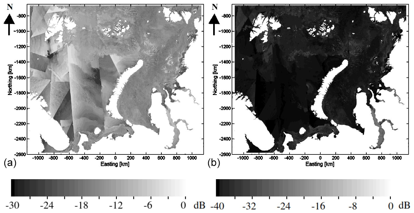
Figure 4Sentinel-1 HH (a) and HV (b) mosaic σ0 segment median on 21 February 2017.

Figure 5Cropped area of the HH (a) and HV (b) segment median images of Fig. 4.
The mosaic was initialized only in the beginning of the mosaicking (in this case in the beginning January 2016). In practice the data at a given grid cell location were never older than 3 d from the mosaic time label. Separate mosaics for the HH and HV channels were constructed. Finally, a land mask based on the Global Self-consistent, Hierarchical, High-resolution Geography Database (GSHHG) coastline (Wessel and Smith, 1996) was applied to the mosaics. The SAR mosaics of 21 February 2017 for the HH and HV channels are shown in Fig. 4 and small parts of the mosaics (more details visible) in Fig. 5.
SAR images were processed to 8 bits-per-pixel images by scaling the σ0 between 1 and 255 (0 representing background). The scaling for the HH channel is such that −30 dB corresponds to the pixel value of 1 and 0 dB corresponds to the pixel value of 255. For the HV channel the decibel values are −40 and 0, respectively. For segmentation the meanshift (MS) algorithm (Fukunaga and Hostetler, 1975) was first applied to locate the modes of the two-dimensional (HH and HV) SAR data. The meanshift algorithm has been empirically adjusted so that about 10–15 modes will be produced after convergence. The initial 10–15 categories based on MS were then used as a starting point for iterated conditional mode (ICM) segmentation (Besag, 1986).
We also identify the low-SIC areas (SAR segments with SIC < 50 %) and exclude them from the SIT estimation procedure. The algorithm utilizing both SAR and AMSR2 microwave radiometer data of Karvonen (2017) is used to locate the low-SIC areas.
In the first sub-section we describe the SAR processing including calibration, resampling to the desired projection and cropping to the study area, and building daily SAR mosaics. Interpolation of the CS2 SIT is then described in the following subsection. This interpolation consists of several steps, including SAR segmentation and computing segmentwise SAR texture features used in the matching of the SAR segments used to define the SIT value to be assigned to each SAR segment. In the third subsection we describe the remapping of the SIT applied here to better correspondence between the estimated SIT and modelled SIT.
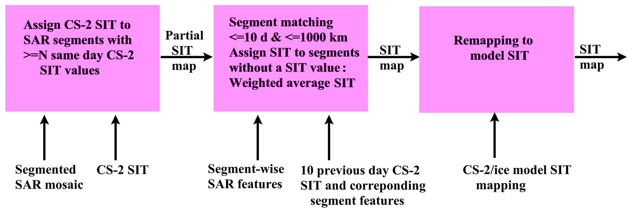
Figure 6Algorithm block diagram for the sea ice thickness estimation using combination of the CryoSat-2 sea ice thickness data and Sentinel-1 SAR imagery. We have used N=7 in this study.
A block diagram of the SIT estimation algorithm is presented in Fig. 6. In the first phase the CS2 SIT values are assigned to segments of the segmented SAR mosaic. Only the segments with a large enough number of CS2 SIT measurements (≥N) within them get a SIT directly assigned. The SIT value assigned to the segments is the median of the CS2 SIT values within the segment. In the next phase a difference function to other segments with CS2 SIT measurements and with a predefined distance and time range is computed for all the segments without an assigned SIT value yet. The difference function describes the pairwise segment similarity, which is small for similar segments and larger for different segments. In the following phase a SIT is interpolated to the segments without a SIT value based on the CS2 SIT values within the similar segments. For one segment the SIT values of the segments ordered by ascending similarity (difference function) with respect to the segment are used to interpolate the SIT for the segment. The CS2 SIT values of the most similar segments are included until the number of SIT values exceeds the threshold value N. The average of these included CS2 SIT values weighted by the inverse of the segment difference is then assigned to the segment. For the remapped estimates a mapping based on histograms of the estimated SIT and PIOMAS ice model SIT for training data is performed to get reduced bias with respect to the reference data. These steps are described in more detail in the following subsections.
4.1 Interpolation of CS2 SIT using S-1 SAR
In this subsection we describe the mapping and interpolation of the CS2 SIT to SAR segments. SAR segments represent uniform areas in the SAR image, and each SAR segment is here assumed to have a uniform SIT value derived from the CS2 SIT values within the segment or interpolated from the CS2 SIT values of other SAR segments with CS2 SIT values in case there are not enough CS2 SIT values within a SAR segment.
As we want to provide SIT estimates for uniform areas of the SAR mosaics, i.e. SAR segments, the mosaics first need to segmented. After segmentation the CS2 SIT values are mapped to SAR segments where enough single CS2 SIT measurements are available. The SIT value assigned to these segments is the median value of the CS2 SIT values within the segment. Then the SIT is estimated (interpolated) for the rest of the segments by utilizing a difference function describing the similarity of the segments and pairwise distance of each pair of segments in time and space. The difference function includes difference of several SAR texture features in addition to the temporal and spatial pairwise distance of the segments. The data of January–April and October–December 2016 were used for training the algorithm and January–April and October–December 2017 data were used for evaluating the algorithm performance.
The SAR features were computed within a round-shaped window with a radius R. In this study we have used R=5 pixels. The median of the feature values within each segment was then assigned to the segments as segmentwise texture features. The features used in this study are as follows.
-
HH backscattering coefficient ( in decibels)
-
HV backscattering coefficient ( in decibels)
-
HH entropies (EHH)
-
HV entropies (EHV)
-
HH local autocorrelations ()
-
HV local autocorrelations ()
-
HH/HV channel cross-correlation (Cc)
-
HH local variogram slopes ()
-
HV local variogram slopes ()
-
HH coefficient of variations ()
-
HV coefficient of variations ()
-
HH edge point densities ()
-
HV edge point densities ()
-
HH corner point densities ()
-
HV corner point densities ()
The feature computation windows were overlapping by half of the window size (i.e. window radius) in both coordinate directions.
Entropy E (Shannon, 1948) was computed as
where pk values are the proportions of each grey tone k within each computation window. Auto-correlation CA (Box and Jenkins, 1976) was computed as
where I(k,l) is the pixel value at image location (k,l). Mean over the horizontal, vertical and diagonal directions i.e. , , and , was used to accomplish directional independence. The computation window is here denoted by W. σW and μW are the mean and standard deviation within the window, respectively.
The cross-correlation Cc (Knapp and Carter, 1976) between the SAR polarization channels (HH and HV), here denoted by X (HH) and Y (HV), is
where k and l refer to the row and column coordinates of the window centre image pixel, respectively; σx and μx are the mean and standard deviation, respectively, of the window in X; and σy and μy are the mean and standard deviation, respectively, of the window in Y. Np is the number of pixels within the window denoted by W.
We also computed texture features based on local variograms. The variograms were locally estimated in a window with a radius of 5 pixels. Assuming a stationary and isotropic process, the variogram γ is (locally) dependent on the inter-distance, here denoted by d, only (Cressie, 1993) and can be estimated as
where zi and zj are the pixel values at locations i and j, whose distance is d; Nd is the set of pixels with the mutual distance d; and is the number of these pixels within the window. We have computed the length of an approximately linear part of the variogram as a function of h and the slope of a linear fit of this linear part. These are referred to here as features and , where ch (channel) is either HH or HV.
The coefficient of variation is computed as
where σ and μ are the standard deviation and mean within the window w. Cv is computed separately for the HH and HV channels, respectively; i.e. we have and .
Edge and corner points represent the locations with large sudden change in σ0, i.e. where high local gradients appear. Corner points are the points where the edge direction abruptly changes. The edge and corner point counts (Ne and Nc) were extracted for each segment using local binary patterns (Ojala et al., 1996) in a similar way as presented in Karvonen (2016). The proportion of the number of edge and corner points with respect to each segment area (in pixels) was computed for both polarization channels, and they were used as texture features. These features are denoted here by , , and .
Based on the segmentation result and the SAR texture features complemented by and , the segmentwise median values of each texture feature and channelwise SAR backscattering coefficients were calculated, resulting in a total of 15 SAR features (13 texture features and two backscattering coefficients) for each segment. As an example, segmented SAR mosaics with and medians assigned to SAR segments on 21 February 2017 are shown in Fig. 4, and details of these HH and HV mosaics are shown in Fig. 5. We use the SIT estimation and reference SIT data of this day as an example in the following sections.
The segment difference function T was defined as the linear combination of the SAR feature differences and temporal and spatial distance between a segment pair:
Δt is the (absolute) time difference in days, ΔD is the distance difference between the centres of the segments and Δfk is the difference between a SAR feature fk (k=1, …, 15) in the two segments. The 2016 CS2 thickness and SAR mosaics (training data) were used in defining the coefficients ct, cd and ck, using a non-negative least-squares (LS) fit. Non-negative LS was used because all the absolute differences should have an increasing effect on T.
According to our analysis the SIT difference between two segments was mainly explained by the absolute difference, i.e. L1 difference, of a few features. , HV entropy and HH edge density and the spatial distance between segment means were the most significant features based on a least-squares fit of the training data. However, other features also had a minor effect (small but non-zero coefficients based on the LS). For this reason we have used all the above-mentioned features in our difference function because the number of features did not produce any computational problems with respect to execution time or hardware resources on a common desktop personal computer. Because the training data set consisted of data of a whole year with CS2 SIT data (January–April, October–December), we consider this to be a representative training data set and assume there is no significant overfitting.
As training data we used the CS2 SIT values assigned to the segments. Each 2016 training data SAR segment with an assigned SIT was included, and the neighbouring assigned SIT values and the corresponding segment pairwise feature differences were used in the LS fit; i.e. each segment pair with an assigned CS2 SIT was utilized.
SIT for a segment (S) without a SIT value was obtained as follows: T between S and all the other segments within a predefined time and distance range was computed, and the segments were ordered by ascending T. Then the CS2 SIT values of the other segments, in addition to possible CS2 SIT values with segment S (less than N values), were included in a set of SIT values, until the number of the values in the list exceeds the threshold value N (strictly equal to N or more than N). The SIT assigned to S was the weighted average of the SIT values of the collected SIT value set. The weights used in the averaging are relative to the inverse values of T corresponding to the segment from which the SIT values come. The possible (less than N) CS2 SIT values of the segment itself are included with the same weight as the CS2 SIT values within the segment with the smallest non-zero value of T. We have used parameter values of N=7 in this study.
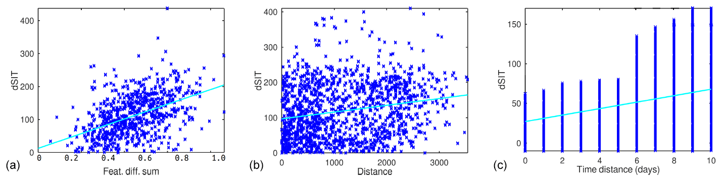
Figure 7(a) Dependence of the SIT difference on the pairwise SAR segment texture difference, (b) dependence of the SIT difference on the pairwise SAR segment distance and (c) dependence of the SIT difference on the pairwise SAR segment time difference. The cyan lines in the figures represent the linear least-squares regression.
In Fig. 7 the dependence of the SIT difference on the SAR feature linear combination, pairwise segment distance and pairwise segment time difference is shown for the 2016 data. Here the time difference is restricted to be less than 1 d (i.e. using only the same day data) and distance less than 500 pixels (250 km) for Fig. 7a, describing the dependence on the pairwise segment texture difference. For Fig. 7b, describing the dependence of the SIT difference on the pairwise segment distance, and Fig. 7c, describing the dependence of the SIT difference on the segment time difference, the normalized pairwise texture difference is restricted to be under 0.1. For Fig. 7b the time difference less than 1 d, and for Fig. 7c the distance difference is restricted to be less than 250 km. It can be seen that there is a clear correlation between the linear combination of the texture feature differences and the SIT difference. There is quite a large deviation; however, the correlation is around 0.5. For the pairwise segment distance and the pairwise segment time difference, correlations are smaller (0.28 and 0.22, respectively), but there is still a visible trend. Based on the slopes of the linear fits, the average increase in SIT difference is 2.9 cm (100 km)−1 and 2.1 cm d−1.
4.2 Ice chart and model-compliant CS2 product
After defining the coefficients ct, cd and ck in Eq. (9) using the training data, we tested the SIT estimation for the 2016 training data. It was observed that SIT is significantly overestimated in the 2016 training data when compared to the modelled and AARI SIT. Therefore, we introduce a mapping based on the PIOMAS model reanalysis SIT data to reduce this SIT overestimation. The CS2 SIT measurements are now further mapped based on the training data and the corresponding PIOMAS reanalysis SIT. The coarser-resolution PIOMAS data were selected for this purpose because ORAS5 does not give reasonable SIT values for SIT less than 50 cm (Tietsche et al., 2017). The adapted SIT histogram mapping is based on the normalized histograms and minimizing the Kolmogorov–Smirnov distance (i.e. mapping the cumulative histograms) of the CS2/S-1 SIT and the TOPAZ4 reanalysis SIT. The Kolmogorov–Smirnov distance, Dm, for a variable x is defined as
where supx is the supremum within the range of x (SIT in our case), and Ft(x) and Fc(x) are the cumulative probability density functions (CDFs) of the PIOMAS SIT and CS2 SIT computed for the 2016 training data set. In our case we have quantized the SIT into integer centimetres with 16 bits, and the SIT histograms are used as approximations of probability density functions (PDFs).
This mapping based on the 2016 training data CS2 SIT and PIOMAS model SIT is shown in Fig. 8 as a green curve, For reference the AARI ice chart SIT, ORAS5 model SIT and TOPAZ4 model SIT (blue curve) matching results are also shown in Fig. 8. It can be seen that TOPAZ4 reanalysis SIT mapping is at a significantly lower level than the mapping for the other two models.
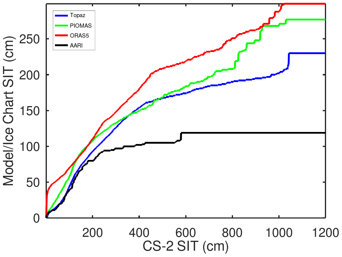
Figure 8The correspondence of the CryoSat-2 SIT to AARI ice chart SIT and modelled SIT from the three models studied based on histogram matching.
5.1 Measures used in evaluation of the results
We have compared the SIT values produced by the CS2/S-1 algorithm to the SIT based on the AARI ice charts, ORAS5, PIOMAS and TOPAZ4 reanalysis to evaluate the algorithm performance. In the comparisons we have used the following measures of difference between the CS2/S-1 SIT estimates and the reference SIT:
Ns refers to the number of samples (number of grid points involved) used in the comparison, and Xi (i=1, …, Ns) represents the estimated values of SIT and represents the values of the reference SIT data at the same location as Xi. C is the correlation, DL1 is the L1 difference and Dsgn is the signed L1 difference giving the estimation bias, with positive bias indicating overestimation and negative bias indicating underestimation. DRMS is the root-mean-square difference. μ and μref are the means of the estimated SIT and reference SIT, and σ and σref are the standard deviations of the estimated SIT and reference SIT, respectively. All the difference measures were computed in the resolution of each reference data set; i.e. the CS2 SIT assigned to SAR segments and interpolated, given in a high-resolution grid, were down-sampled to each reference data set resolution. This approach was not applicable to the single CS2 SIT measurements, and for them the difference measures were computed directly, using the nearest reference data set grid point SIT for each measurement as the reference SIT.
As the CS2 SIT data cover only the time period from October to April, the weather conditions were mostly with dry snow conditions; i.e. Ta was mainly below 0∘ for the time range studied. Only in the early winter (October–November) there were some periods with Ta above zero and the potential to have wet snow on sea ice. In this study we do evaluate the effect of wet snow on the SIT estimation. For reliable estimation of the effect of wet snow conditions on estimation, more data acquired during the melting period would be required.
5.2 Difference statistics between the estimates and reference data
The statistics from the comparisons between the CS2/S-1 SIT, without and with the proposed histogram mapping, and the different reference SIT data sets are shown in Tables 1–4. The correlations between different SIT data sets for each 2017 winter month and their averages and standard deviations are shown in Table 1, the corresponding biases in Table 2, the L1 differences in Table 3 and the RMSDs in Table 4. For reference, the average difference measures and correlations between the different reference SIT data sets are shown in Table 5.
Table 1Monthly average cross-correlations between the SIT estimates studied with respect to the reference data set SIT. SIT refers to the proposed algorithm SIT, RSIT refers to the proposed algorithm SIT with remapping based on the histogram mapping with model data, CS2 refers to the CS2 values assigned to the SAR segments (without inter- or extrapolation), A refers to the SIT derived from the AARI ice charts, T refers to the TOPAZ4 model reanalysis SIT, and O refers to the ORAS5 model SIT.

Table 2Monthly average bias in centimetres between the different SIT estimates with respect to the SIT reference data sets. The symbols are the same as in Table 1.
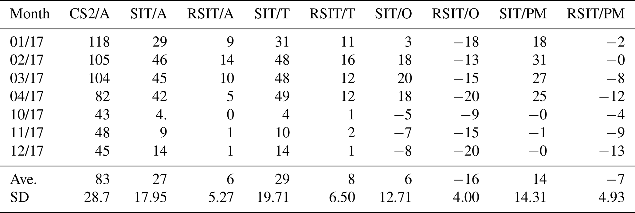
Table 3Monthly average L1 difference in centimetres between the different SIT estimates with respect to the reference SIT data sets. The symbols are the same as in Table 1.
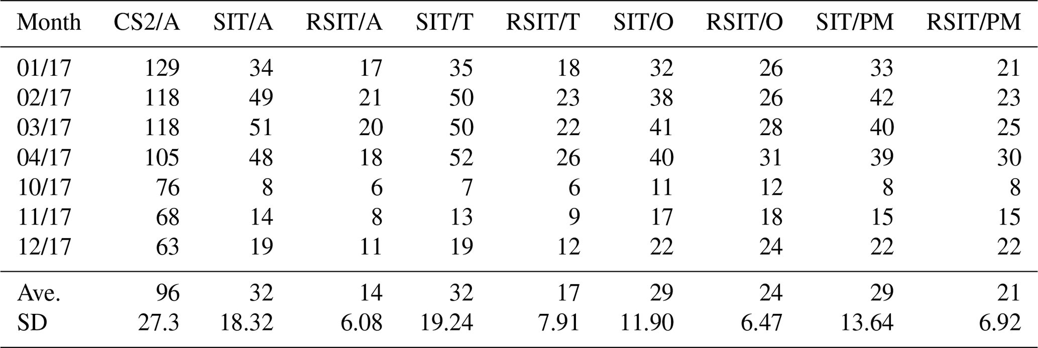
Table 4Monthly average RMSD in centimetres between the different SIT estimates with respect to the reference SIT data sets. The symbols are the same as in Table 3.
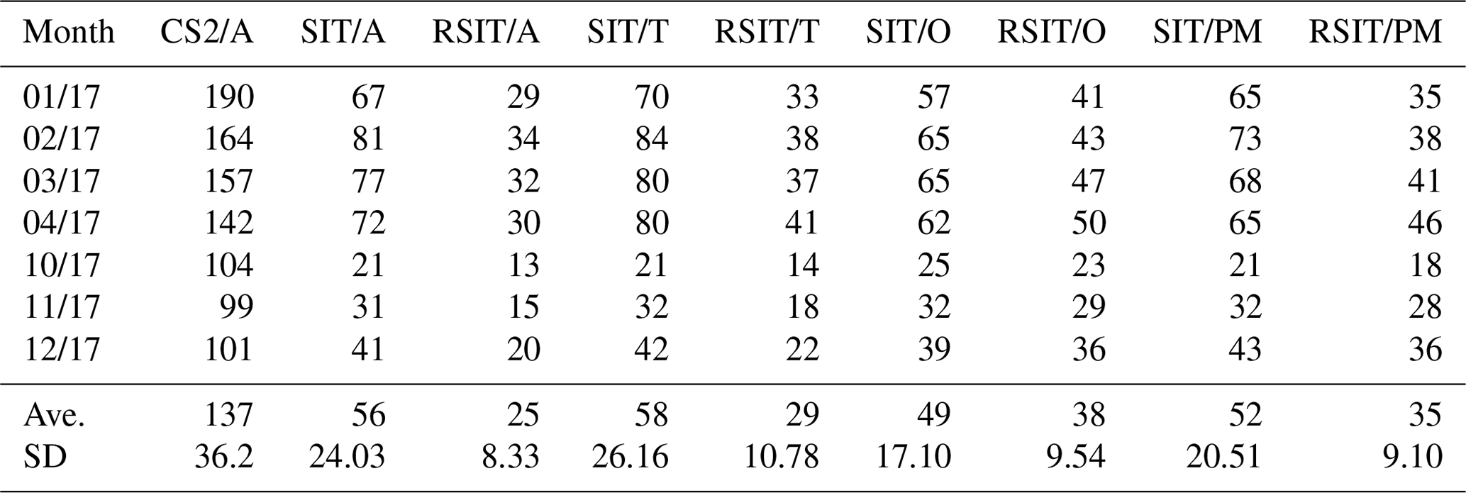
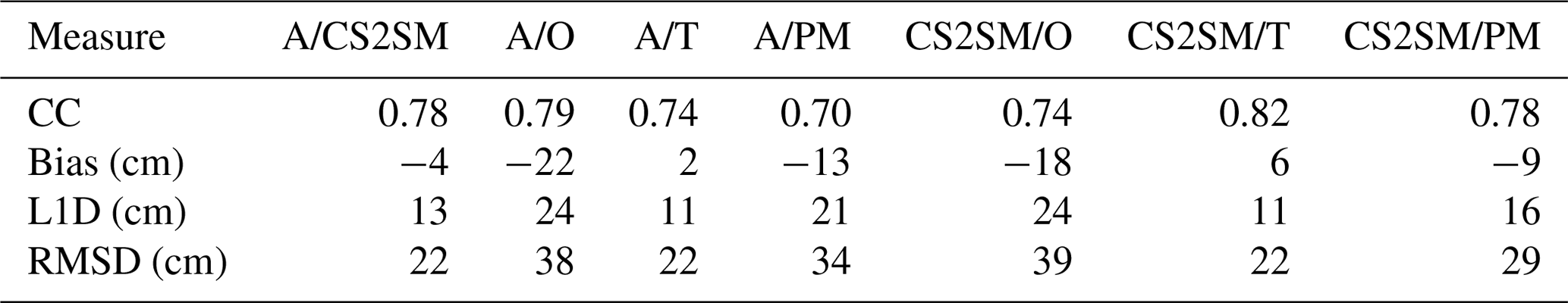
Table 5Average difference measures between the AARI ice chart SIT (A), CS2SMOS SIT (CS2SM) and SIT of the three ice models. O refers to ORAS5, T refers to TOPAZ4 and PM refers to PIOMAS.
On average the correlation between the non-interpolated CS2 SIT estimates and the AARI ice chart SIT was very small, only 0.15. There was a significant bias, CS2 SIT being on average 83 cm larger than the AARI chart SIT. This also reflects the high L1 differences and RMSDs between the CS2 and AARI SITs. The statistics of the CS2 SIT with respect to the AARI SIT are given in the first columns of Tables 1–4. The numbers were similar with respect to the three ice models, showing small correlations and large positive bias (overestimation by CS2). Because of their similarity these values were not included to the tables.
The correlations for the interpolated CS2 SIT assigned to the SAR segments was significantly higher, around 0.64. The monthly correlations between the interpolated CS2/S-1 SIT and the remapped interpolated CS2/S-1 SIT with respect to the AARI SIT were similar and in the range 0.52–0.76. The highest values were reached in April and October. There CS2/S-1 SIT correlations were quite similar with respect to the model data for all the studied models.
The monthly signed L1 difference in Table 2 also increases for the estimated SIT with respect to both the AARI SIT and model reanalysis SIT as the ice gets thicker, indicating significant overestimation. For the remapped interpolated SIT, bias remains at a lower level for all the studied months. With respect to ORAS5 there was even small underestimation on average, but with respect to TOPAZ4 reanalysis SIT there was some overestimation. The averages and maximum biases for the interpolated SIT with respect to the AARI SIT were 27 and 46 cm (maximum reached in March). The corresponding values with respect to the AARI SIT for the remapped interpolated SIT were 6 and 14 cm (maximum underestimation in April). The corresponding values with respect to the TOPAZ4 reanalysis SIT were 29 and 49 cm and 8 and 16 cm, respectively. The corresponding values with respect to the ORAS5 SIT were 6 and 20 cm and −15 and −20 cm, i.e. slight underestimation. For the PIOMAS model data the corresponding figures were 14 and 31 cm and −7 and −13 cm.
The monthly L1 differences in Table 3 were smaller for the freeze-up period and higher for the winter months, starting to decrease in April. The L1 differences with respect to the AARI SIT and TOPAZ4, ORAS5 and PIOMAS reanalysis SIT were smaller for the remapped estimated SIT, which was expected as the target of the remapping was to reduce the relatively large positive bias. The average and maximum L1 differences with respect to AARI SIT were 32 and 51 cm for the interpolated SIT and 14 and 21 cm for the remapped interpolated SIT. The maximum values were reached in January and March. The corresponding values with respect to TOPAZ reanalysis were 32 and 52 cm and 17 and 26 cm, with respect to ORAS5 SIT 29 and 41 cm and 24 and 31 cm, and with respect to PIOMAS SIT 29 and 42 cm and 21 and 30 cm. The difference maxima were reached in February–April for all the cases.
The RMSDs in Table 4 have a similar behaviour as the L1 differences. RMSD also increases as the average ice thickness increases in the course of the winter, and the smallest RMSD values were reached during the freeze-up months (October–December). The average and monthly maximum RMSD values for the estimated SIT with respect to the AARI SIT were 56 and 81 cm, and the corresponding values for the remapped estimated SIT were 25 and 34 cm. The corresponding values with respect to the TOPAZ4 reanalysis SIT were 58 and 84 cm for the interpolated SIT and 29 and 41 cm for the remapped interpolated SIT. The corresponding values with respect to the ORAS5 SIT were 49 and 65 cm for the estimated SIT and 38 and 50 cm for the remapped interpolated SIT. The corresponding values with respect to PIOMAS SIT were the 52 and 73 cm for the estimated SIT and 35 and 46 cm for the remapped interpolated SIT. The average maxima were again reached during the winter months (January–April).
For the CS2 SIT the difference measures shown in Tables 2–4 indicate large positive biases (overestimation) and large L1D and RMSD with respect to the AARI SIT, TOPAZ4, ORAS5 and PIOMAS reanalysis SIT. These values are highest for the winter months with the thickest ice and smaller for the freeze-up/early winter (October–December). The cross-correlations with respect to all reference data sets were low, significantly lower than for the interpolated CS2/S-1 SIT.
It should be noted that the reference SIT data sets also differ from each other; see Table 5. The average cross-correlations between the reference data sets were in the range 0.54–0.60. The TOPAZ4 and AARI SIT values were on average quite close to each other, having only low bias, but the ORAS5 SIT was then on average 35–40 cm above them. Furthermore, it is noted that in our evaluation the compared randomly sampled points were located in highly dissimilar regions, characteristic for the different data sets, with different sizes and shapes (such as ice model grid points, SAR segments, ice chart polygons).
In order to assess how far from the assigned CS2 measurement the SIT can be interpolated and still give usable estimates, we studied the effect of distance and time on the SIT difference (or in other words, estimation error) using our training data set. We used the assigned CS2 SIT values as reference and searched for sets of segments with either constant time difference or constant distance and defined the increase in SIT difference as a function of the difference in the other. The average increase in estimation error for the training data set as a function of time was 2.1 cm d−1 and of distance was 2.9 cm (100 km)−1. This indicates that the contribution of distance difference to the total difference is at a maximum (corresponding to the search range boundaries) around 14 cm for the 1000 pixel (500 km) spatial search range and 21 cm for the 10 d temporal search range.
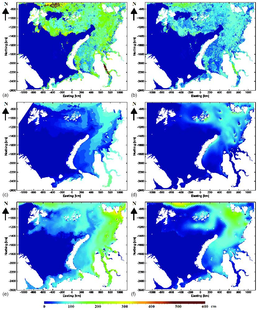
Figure 9(a) CS2/S-1 SIT, (b) remapped CS2/S-1 SIT, (c) AARI ice chart SIT, (d) TOPAZ4 ice model reanalysis SIT, (e) ORAS5 model ice model SIT and (f) CS2/SMOS SIT for 21 February 2017.
An example of the SIT estimation on 21 February 2017 without and with the histogram remapping can be seen in Fig. 9. For reference the AARI SIT and TOPAZ4, ORAS5 reanalysis SIT, and CS2SMOS SIT have also been included in Fig. 9. This figure represents a typical case of the thinner and thicker ice fields generally in agreement with the reference data but still indicating differences due to the details of the local SIT distribution, given at a higher level of detail in the estimated CS2/S-1 SIT.
Table 6Comparison between the CS2 SIT assigned to SAR mosaic segments and CS2SMOS SIT.
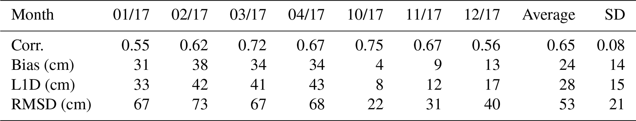
Table 7Comparison between the CS2 assigned to SAR mosaic segments with the mapping and CS2SMOS SIT.
We also included a comparison of the proposed SIT estimates (interpolated and remapped versions) to the CS2SMOS SIT data (Ricker et al., 2017) for our 2017 test data set. These comparison results are shown in Tables 6 and 7. The results are discussed more in the following subsection.
5.3 Difference maps and estimation uncertainty
We also provide difference maps of the unmapped and remapped SIT with respect to the AARI ice chart SIT in Fig. 10 for the 21 February 2021 case and for the 2017 test data set on average. It can be seen that the unmapped interpolated SIT overestimates SIT with respect to the AARI ice chart SIT, for both the 21 February 2017 case and the average in many areas. For the remapped interpolated SIT estimates the overestimation is significantly smaller with respect to the AARI ice chart SIT for both the case of 21 February 2017 and on average.
Figure 10(a) Difference of the proposed (unmapped) SIT for 21 February 2017 and AARI ice chart SIT, (b) difference of the proposed remapped SIT and AARI ice chart SIT for 21 February 2017, (c) average difference of the proposed (unmapped) SIT and the AARI ice chart SIT for the 2017 data, and (d) average difference of the proposed remapped SIT and the AARI ice chart SIT for the 2017 data.
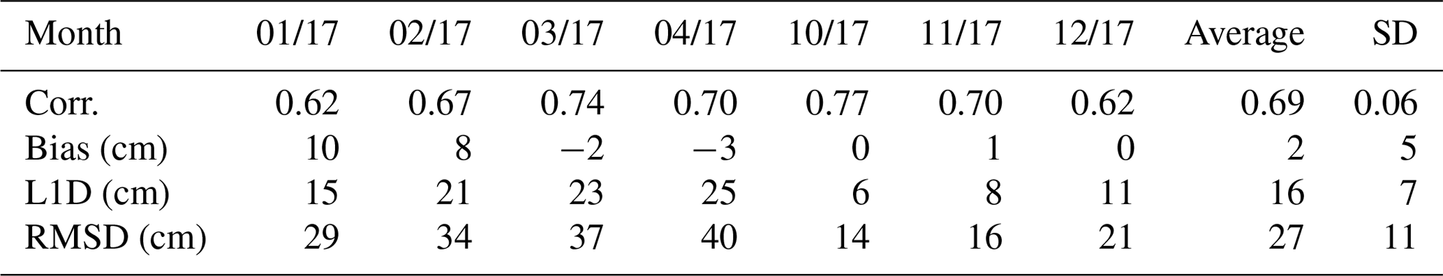
Figure 11(a) Difference of the proposed (unmapped) SIT and CS2SMOS SIT for the 21 February 2017 case, (b) difference of the proposed remapped SIT and CS2SMOS SIT for the 21 February 2017 case, (c) average difference of the proposed (unmapped) SIT and the CS2SMOS SIT for the 2017 data, and (d) average difference of the proposed remapped SIT and the CS2SMOS SIT for the 2017 data.
SIT difference charts with respect to the CS2SMOS SIT on 21 February 2017 and the average difference charts for 2017 are shown in Fig. 11. It can be seen that the SIT differences are quite similar to the differences with respect to the AARI ice charts. There is some more underestimation in the northeastern part of the study area compared to the difference maps with the AARI SIT. This comparison also indicates that the interpolated SIT estimates deem to overestimate SIT, and the remapped interpolated SIT values are less biased.
As we are using a (segment) difference function for each segment, this value corresponds to the mapping and the larger it is the larger the uncertainty of the SIT estimation can be considered. We have scaled the difference T values to the range 0–100 (based on the training data difference function values), and in Fig. 12 the scaled difference function for 21 February 2017 is shown. The highest uncertainty is found at the ice edge and in the Ob River delta area. The uncertainly could probably also be used for iteratively re-estimating the SIT of segments with the highest uncertainties.
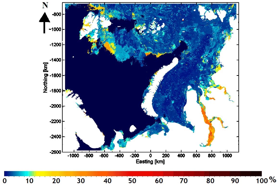
Figure 12Segment difference (T) as a measure of uncertainty of the SIT estimates. This is the segment difference for the 21 February 2017 case. The values of T have been scaled to the range 0–100, based on the variation in T in the training data. The black area is open water.
5.4 Comparison to MODIS SIT
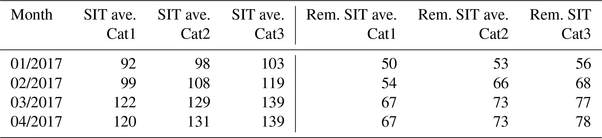
We also performed comparisons of the interpolated CS2/S-1 SIT estimates against the daily MODIS SIT charts. The MODIS product only gives thin-ice thicknesses, and the thicker ice thicknesses are only roughly categorized: SIT in the 1–30 cm range and then one category for SIT of 31–50 cm and another for SIT over 50 cm. The monthly correlations between the thin MODIS SIT (1–30 cm) and the SIT estimated by the proposed method varied between 0.15 and 0.25. We also computed the averages of the estimated SIT for the three MODIS SIT categories for each month and for the estimated SIT and estimated remapped SIT. These are presented in Table 8. It can be seen that the averages increase towards a thicker MODIS thickness category for both the estimates, but the increases are quite small and the averages are high for both the methods, some less for the remapped estimate. It can also be seen that the averages increase as a function of time, i.e. as ice gets thicker in the course of time. Based on this experiment we can conclude that the SIT estimates, even with the proposed remapping, tend to overestimate SIT, specifically for thin ice.
Table 8Monthly averages of estimated SIT (SIT) and remapped SIT (Rem. SIT) for the MODIS daily SIT chart categories. All values are in centimetres. The MODIS SIT categories are 1–30 cm (Cat1), 31–50 cm (Cat2) and over 50 cm (Cat3).
For visual evaluation and comparison to the SIT estimates of Fig. 9, we also show the MODIS SIT collage for 21 February 2017 in Fig. 13. For better visual appearance the colour scale is different from that of Fig. 9. Because in a daily MODIS SIT chart SIT can typically be computed only for small areas due to cloud cover, the collage is composed of 2 weeks of MODIS SIT charts with the most recent available MODIS SIT value at each grid point. The areas with no data during the 2-week period are indicated by the black colour in the figure.When comparing the MODIS SIT collage of Fig. 10 with the daily CS2/S-1 SIT estimate in Fig. 8b, we notice that most of the ice-covered regions of the study area belong to the thickest MODIS SIT category (SIT > 50 cm). The thin-ice areas according to the MODIS SIT are located near the Kara Gate (southern Kara Sea) and near the ice edge in the northwestern part of the study area. These are in general in agreement with the CS2/S-1 SIT. Also, some thicker ice patches within or in the vicinity of the MODIS SIT thin-ice areas can be identified in the CS2/S-1 SIT. The general pattern detecting thinner ice in the south and near the ice edge is present in both CS2/S-1 and MODIS SIT. This general large-scale pattern can be seen throughout the winter. However, the SIT estimates include many anomalous local details due to the dynamic nature of the ice field and the fact that the data are not exactly simultaneous.
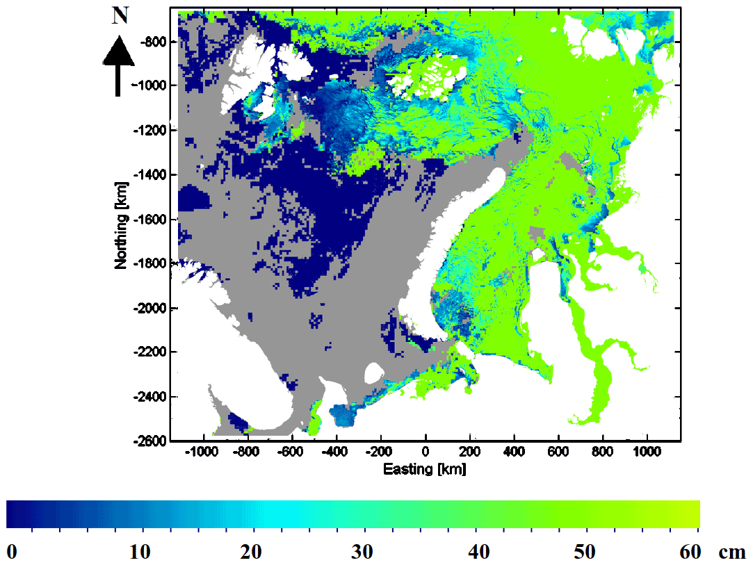
Figure 13MODIS SIT collage based on 2 weeks of MODIS daily SIT charts before 21 February 2017. The areas without data are indicated by the grey colour, and all the ice thicker than 50 cm is indicated by the green colour, corresponding to 60 cm in the colour map.
In this study an algorithm for interpolating the CS2 SIT data over the daily Kara Sea and Barents Sea S-1 SAR mosaic was developed and evaluated by comparisons to SIT derived from the AARI ice charts and three ice model reanalysis data sets. Baseline-D CS2 data (Meloni et al., 2020) were used in this study. Baseline-D data were was the most recent version when our data analysis was made. We wanted to demonstrate the potential of our method, as well as to evaluate its performance. Our method is capable of interpolating CS2 SIT values to areas between orbit ground tracks where SIT measurements are not available. We found significant differences (low correlation, large bias) between non-interpolated CS2 SIT and the reference data. Given the different nature of our reference data, this was not surprising. The match between CS2 and reference data improved with the introduction of segmentwise medians. However, there were still significant differences, especially a high positive bias due to different nature of CS2 SIT estimates and the reference SIT data sets. To reduce this bias, we performed a mapping based on the PDFs (histograms) of the CS2 SIT and PIOMAS ice model reanalysis SIT for our training data set. This mapping reduced the positive bias, which also reflected the reduced L1D and RMSD. However, the remapped CS2 data should not be understood as more correct but as more akin to the model SIT.
We used the 2016 data (January–April, October–December) as the training data set and 2017 data (January–April, October–December) as a test data set in this study. There would have been different ways of dividing the data into the training and test data sets, e.g. randomly selected days or one whole season for training instead of using calendar year data from two seasons. However, with some preliminary tests this did not have any significant effect on the results, and we selected this chronological order (training data earlier than test data) for this study. The training and evaluation of this study were also performed for January–April and November–December. This was because both the CS2 SIT and AARI ice chart ice stage of development were not available outside of this period, i.e. under wet surface conditions. For such conditions reliable estimation of SIT is difficult or even impossible with the current data and algorithms. This is due to the deviating behaviour of radar signal at the wet air–snow/ice boundary, compared to a frozen surface.
An alternative to directly using CS2 SIT would have been to utilize CS2 ice freeboard. Then ice freeboard could have been computed from modelled ice and snow data using Eq. (1). Freeboard could be a more suitable quantity for comparisons because radar backscatter and ice freeboard are statistically related as reported in Simila et al. (2010). The radar penetrates the snow layer, and radar backscattering is from the ice surface layer in dry snow conditions. Using ice freeboard can also reduce the effect of incorrect snow depth.
An interesting result was that the interpolation does not decrease the correlation with respect to the reference data compared to (incomplete) SIT resulting from CS2 data assigned to SAR segments, or CS2 data as individual measurements. For example, the correlation for the CS2 SIT assigned to segments with respect to the AARI ice chart SIT was on average around 0.64. This is a similar value as for the interpolated segmentwise CS2 SIT. For the individual pointwise CS2 SIT values the correlations were significantly lower.
In parts of the study area there may be areas with wet snow on sea ice (Rösel et al., 2018). Wet snow will have an effect on the SIT estimate accuracy in late winter. Because the CS2 SIT is produced for the winter months only, i.e. stopped at the end of April, indicating that most of the melt-down period, most likely to have wet snow on ice, is excluded. In this study the uncertainty due to wet snow was not studied, but this will be an interesting topic for further studies.
In general, evaluation of ice thickness over the Arctic is difficult because of a lack of reliable reference data. Another problem is the different scales of the SIT measurements, estimates and models. SIT measurements, if available, are typically point measurements or measurements with a footprint of a few metres to a few tens of metres (e.g. SIT measurements by drilling or electromagnetic-induction-based EM measurements), and the model grid cells, satellite measurements or segmentwise SAR estimates represent averages over several square kilometres (km2). Also, ice charts give averages of typically quite large polygons of several tens or even hundreds of square kilometres.
According to the results the monthly biases without any remapping of the interpolated CS2 SIT are positive with respect to the AARI SIT and smaller but still positive with respect to the ice model data sets. For the remapped interpolated SIT all the biases are smaller. Comparison to the CS2SMOS SIT product with the 2017 test data indicates large overestimation for the interpolated CS2 SIT estimates. This large positive bias was decreased significantly for the remapped estimates and was on average only a few centimetres.
We selected parameters, such as N, empirically. The sensitivity of SIT to parameters chosen was not studied thoroughly yet. It will be a topic for future research. For example the value of N was selected such that we had enough segments with CS2 SIT assigned to them to get interpolated SIT for all the segments of a daily SAR mosaic. Currently the value of N is relatively small for a typical SAR segment. A higher value of N would be preferable. However, a higher value of N in turn would reduce the number of segments included in the estimation and also increase the possibility of too few assigned SIT values for the interpolation step. For this reason we used a moderately small value of N.
The relatively large differences with respect to the reference SIT data sets can at least partly be explained by the different resolutions and level of detail of the SIT estimates. The CS2/S-1 SIT has a resolution of 500 m (the SAR mosaic resolution), which is significantly higher than the resolution of the ORAS5, PIOMAS and TOPAZ4 reanalyses (over 10 km) and also of the AARI ice chart level of detail. Furthermore the original CS2 measurements stem from individual footprints that are approximately 300 m × 1600 m. Even though the ice charts have a nominal resolution up to about 1 km, in practice it is impossible for the ice analysts to include all the ice field details in this scale within the limited time available for making the ice charts. Instead, the ice analysts tend to draw larger polygons, representing rather homogeneous sea ice, neglecting the details and assigning areal average values to the polygons. However, the polygon boundaries typically have the precision of the nominal ice chart resolution. For this reason of varying scales, we have used the reference data resolution in the comparisons and downsampled the interpolated CS2 SIT accordingly. For the individual CS2 SIT measurements, we used the nearest reference grid point data.
We also studied use of regularized linear regression (LASSO) (Tibshiran, 1996) for reducing the number of texture features needed in the SIT estimation. According to our first tests the performance was nearly similar with less texture parameters involved, but on the other hand the need for computational resources with the number of LS fit parameters used now was not significantly larger than with a reduced number of parameters, and thus we here used all the studied parameters in the LS fit in this study. In the future, reduction of LS fit parameters could be studied more, if seen necessary, e.g. for more efficient computing to cover larger sea areas in a reasonable time. This may be required to meet near-real-time processing conditions for operational SIT estimation, e.g. for a pan-Arctic high-resolution SIT product.
Snow depth in winter conditions can be estimated based on microwave radiometer data, e.g. see Rostosky et al. (2018). More precise snow density estimation can then be utilized to yield more precise SIT estimates. Microwave radiometer data can be utilized to locate the thin-ice regions; e.g. AMSR2-based thin-ice (SIT > 20 cm) detection has been recently developed for the Barents and Kara seas. One future goal will be integration of microwave radiometer data in the algorithm to get better estimates of snow cover on sea ice and thin-ice presence.
In some areas near the ice edge there still seems to exist local SIT overestimation with respect to the reference data. One possible way to reduce this overestimation would be to adjust the algorithm parameters such that the spatial search radius would be more restricted near the ice edge, i.e. dependent on the geographical location. This could also be adjusted by varying the weight assigned to pairwise segment distance in the difference function T. However, this alternative will require a significant amount of additional research.
As the proposed method uses several CS2 SIT values to assign a SIT value to a SAR segment, it is also possible to give estimates of the SIT range or SIT distribution of the segments. This does not even require development of new algorithm, only selecting a suitable value of parameter N (number of CS2 SIT values required for a segment) and extracting the SIT range or distribution from the CS2 SIT measurements.
In the future we also plan to study segment clustering and then assigning CS2 SIT value median or mode of each segment cluster to all segments of a segment cluster instead of single segment medians. An easy solution would be to merge small segments into their neighbouring larger segments to remove all the segments smaller than a given area. This would give more CS2 measurements within the segments but on the other hand also then give SIT estimates representing averages of larger areas. Despite this it should be noted that the segment boundaries, representing different ice fields, are still represented in the resolution of the segmentation. With these approaches we aim to overcome the problem of either having too few CS2 SIT values assigned to segments or too few segments with an assigned SIT. Also, more detailed utilization of SIT distributions of segment clusters with a large enough number of SIT samples for forming statistically reliable SIT distributions should be studied. In some cases large SAR segments could also be split into smaller ones to get more detailed and more accurate local SIT estimates.
It may be possible to use the dependence of the biases on the phase of the winter (related to average SIT), such as early freeze-up, freeze-up, mid-winter and early spring phase, to reduce the bias by applying a bias-reducing mapping dependent on the phase of the winter instead of on a common mapping for the whole winter. The phase of the winter could roughly be estimated based on the estimated average ice thickness. Also, different algorithm parameters (weights used in the difference function T) could be tested for different phases of winter. This would require a larger multi-year training data set and a significant amount of additional work but could be one way to improve the SIT estimation accuracy.
Our algorithm can be easily adapted to any satellite altimeter SIT product. This study is especially relevant for the future CRISTAL mission (Kern et al., 2020). After its expected launch in late 2027, CRISTAL shall provide a time-critical SIT product, which can be merged with SAR data to interpolate SIT between the CRISTAL ground tracks. Thus our study is one of the necessary steps in introducing satellite altimeter data into the realm of operational ice charting. Before CRISTAL, our algorithm can be applied to ICESat-2 as well as to Sentinel-3 SRAL-based SIT estimates.
The CS2 data processing was performed using the pysiral SW package (https://github.com/shendric/pysiral/, last access: 11 May 2022; https://doi.org/10.5281/zenodo.5566347, Hendricks et al., 2021b). For access to the SW, contact juha.karvonen@fmi.fi. The original S-1 and CS2 data are available through the ESA Copernicus data hub (https://scihub.copernicus.eu/, last access: 11 May 2022; https://doi.org/10.5281/zenodo.5566347, Hendricks et al., 2021b). The processed data sets (or their subsets) are available only by request to FMI (juha.karvonen@fmi.fi).
JK has developed the algorithm and produced estimation and comparison results and was the main author of the paper. ER and HS performed the CS2 processing and produced the CS2 SIT. They also acted as SAR altimetry experts in the study and writing the paper. MM produced the MOSIT reference SIT data and weather data and acted as a microwave remote sensing expert in the study and writing the paper. PU provided the ORAS5 and PIOMAS model data for the test period and acted as a modelling expert in the study and writing the paper.
The contact author has declared that neither they nor their co-authors have any competing interests.
Publisher’s note: Copernicus Publications remains neutral with regard to jurisdictional claims in published maps and institutional affiliations.
This work was supported in part by the European Union (EU), Finland, Norway, the Russian Federation, and Sweden, through the Kolarctic Cross Border Collaboration (CBC) programme project Ice Operations.
This research has been supported by the European Commission (Kolarctic CBC programme, grant no. KO2100 ICEOP).
Publisher’s note: the article processing charges for this publication were not paid by a Russian or Belarusian institution.
This paper was edited by Ludovic Brucker and reviewed by three anonymous referees.
AARI: AARI ice chart web page, Arctic-Antarctic Research Institute, St. Petersbug, Russia, http://wdc.aari.ru/datasets/d0004/kar/sigrid/ (last access: 10 May 2022), 2018. a
Afanasyeva, E. V., Alekseeva, T. A., Sokolova, J. V., Demchev, D. M., Chufarova, M. S., Bychenkov, Y. D., and Devyataev, O. S.: AARI methodology for sea ice charts composition, Russian Arctic, 7, 5–20, https://doi.org/10.24411/2658-4255-2019-10071, 2019. a, b
Armitage, T. W. K. and Ridout, A. L.: Arctic sea ice freeboard from AltiKa and comparison with CryoSat-2 and Operation IceBridge, Geophys. Res. Lett., 42, 6724–6731, https://doi.org/10.1002/2015GL064823, 2015. a
Besag, J.: On the Statistical Analysis of Dirty Pictures, J. R. Statis. Soc. B, 48, 259–302, 1986. a
Böhme, L. and Send, U.: Objective analyses of hydrographic data for referencing profiling float salinities in highly variable environments, Deep-Sea Res. Pt. II, 52, 651–664, 2005. a
Bourbigot, M., Johnsen, H., and Piantanida, R.: SENTINEL-1 ProductSpecification, document S1-RS-MDA-52-7441, ESA, https://sentinels.copernicus.eu/web/sentinel/user-guides/sentinel-1-sar/document-library/-/asset_publisher/1dO7RF5fJMbd/content/sentinel-1-product-specification (last access: 11 May 2022), 2016. a
Box, G. E. P. and Jenkins, G.: Time Series Analysis: Forecasting and Control, Holden-Day, ISBN 0816211043, 1976. a
Cressie, N.: Statistics for spatial data, Wiley, New York, 69–101, ISBN 9780471002550, 1993. a
Evensen, G.: Sequential data assimilation with a nonlinear quasi-geostrophic model using Monte-Carlo methods to forecast errorstatistics, J. Geophys. Res., 99, 10143–10162, https://doi.org/10.1029/94JC00572, 1994. a
Frey, R. A., Ackerman, S. A., Liu, Y., Strabala, K. I., Zhang, H., Key, J. R., and Wang, X.: Cloud detection with MODIS. Part I: Improvements in the MODIS cloud mask for collection 5, J. Atmos. Ocean. Technol., 25, 1057–1072, 2008. a
Fukunaga, K. and Hostetler, L. D.: The Estimation of the Gradient of a Density Function, with Applications in Pattern Recognition, IEEE T. Inform. Theory, 21, 32–40, 1975. a
Giles, K. A., Laxon, S. W., and Ridout, A. L.: Circumpolar thinning of Arctic sea ice following the 2007 record ice extent minimum, Geophys. Res. Lett., 35, L22502, https://doi.org/10.1029/2008GL035710, 2008. a
Hackett, B., Bertino, L., Ali, A., Burud, A., and Williams, T.: Product User Manual for Arctic Ocean Physical and Bio Analysis and Forecasting Products, issue 5.10, EU Copernicus Marine Service, Public Ref: CMEMS-ARC-PUM-002-ALL, https://marine.copernicus.eu/sites/default/files/product_improvement_migrated_files/CMEMS-ARC-PUM-002-ALL.pdf (last access: 10 May 2022), 2020. a
Hendricks, S., Ricker, R. and Paul, S.: Product User Guide & Algorithm Specification: AWI CryoSat-2 Sea Ice Thickness (version 2.4), EU Copernicus Marine Service, Public Ref: CMEMS-ARC-PUM-002-ALL, https://epic.awi.de/id/eprint/54733/ (last access: 11 May 2022), 2021a. a
Hendricks, S., Sallila, H., Brockley, D., and Paul, S.: shendric/pysiral: Product update (C3S, AWI, CCI, CryoTEMPO) (v0.9.6), Zenodo [data set], https://doi.org/10.5281/zenodo.5566347, 2021b. a, b
Huntemann, M., Heygster, G., Kaleschke, L., Krumpen, T., Mäkynen, M., and Drusch, M.: Empirical sea ice thickness retrieval during the freeze-up period from SMOS high incident angle observations, The Cryosphere, 8, 439–451, https://doi.org/10.5194/tc-8-439-2014, 2014. a
IMarEST: Safety & Sustainability of Shipping and Offshore Activities in the Arctic, Institute of Marine Engineering, Science & Technology, IMarEST Report, London International Shipping Week, https://www.imarest.org/reports/731-imarest-arctic-roundtable-report/file (last access: 11 May 2022), 2015. a
Iwamoto, K., Ohshima, K. I., and Tamura, T.: Improved mapping of sea ice production in the Arctic Ocean using AMSR-E thin ice thickness algorithm, J. Geophys. Res., 119, 3574–3594, 2014. a
JCOMM Expert Team on Sea Ice: Sea-ice nomenclature: Snapshot of the WMO sea ice nomenclature, WMO no. 259, Joint WMO-IOC Commission for Oceanography and Marine Meteorology, Tech. Rep., World Meteorological Organization (WMO), Geneva, Switzerland, https://doi.org/10.25607/OBP-1515, 2014a. a, b
JCOMM Expert Team on Sea Ice: SIGRID-3: a vector archive format for sea ice georeferenced information and data, Joint WMO-IOC Commission for Oceanography and Marine Meteorology, Technical Report No. 23, World Meteorological Organization (WMO), Geneva, Switzerland, https://doi.org/10.25607/OBP-1498.2, 2014b. a
Johannessen, O. M., Alexandrov, V. Y., Frolov, I. Y., Sandven, S., Pettersson, L. H., Bobylev, L. P., Kloster, K., Smirnov, V. G., Mironov, Y. U., and Babich, N. G.: Remote sensing of sea ice in the northern sea route: studies and applications, Springer-Praxis, Chichester, UK, 25–64, ISBN 9783540488408, 2007. a, b
Jung, T., Kasper, M. A., Semmler, T., and Serrar, S.: Arctic influence on subseasonal midlatitude prediction, Geophys. Res. Lett., 41, 3676–3680, 2014. a
Kaleschke, L., Tian-Kunze, X., Maaß, N., Makynen, M., and Drusch, M.: Sea ice thickness retrieval from SMOS brightness temperatures during the Arctic freeze-up period, Geophys. Res. Lett., 39, L05501, https://doi.org/10.1029/2012GL050916, 2012. a, b
Kaleschke, L., Tioan-Kunze, X., Maass, N., Beitsch, A., Wernecke, A., Miernecki, M., Muller, G., Fock, B. H., Gierischc, A. M. U., Schlunzen, K. H., Pohlmann, T., Dobrynin, M., Hendricks, S., Asseng, J., Gerdes, R., Jochmann, P., Reimer, N., Holfort, J., Melsheimer, C., Heygster, G., Spreen, G., Gerland, S., King, J., Skou, N., Søbjærg, S. S., Haas, C., Richter, F., and Casal, T.: SMOS sea ice product: Operational application and validation in the Barents Sea marginal ice zone, Remote Sens. Environ., 180, 264–273, 2016. a, b
Karvonen, J.: Virtual radar ice buoys – a method for measuring fine-scale sea ice drift, The Cryosphere, 10, 29–42, https://doi.org/10.5194/tc-10-29-2016, 2016. a
Karvonen, J.: Baltic Sea Ice Concentration Estimation Using SENTINEL-1 SAR and AMSR2 Microwave Radiometer Data, IEEE T. Geosci. Remote, 55, 2871–2883, 2017. a, b
Kern, S., Khvorostovsky, K., Skourup, H., Rinne, E., Parsakhoo, Z. S., Djepa, V., Wadhams, P., and Sandven, S.: The impact of snow depth, snow density and ice density on sea ice thickness retrieval from satellite radar altimetry: results from the ESA-CCI Sea Ice ECV Project Round Robin Exercise, The Cryosphere, 9, 37–52, https://doi.org/10.5194/tc-9-37-2015, 2015. a
Kern, M., Cullen, R., Berruti, B., Bouffard, J., Casal, T., Drinkwater, M. R., Gabriele, A., Lecuyot, A., Ludwig, M., Midthassel, R., Navas Traver, I., Parrinello, T., Ressler, G., Andersson, E., Martin-Puig, C., Andersen, O., Bartsch, A., Farrell, S., Fleury, S., Gascoin, S., Guillot, A., Humbert, A., Rinne, E., Shepherd, A., van den Broeke, M. R., and Yackel, J.: The Copernicus Polar Ice and Snow Topography Altimeter (CRISTAL) high-priority candidate mission, The Cryosphere, 14, 2235–2251, https://doi.org/10.5194/tc-14-2235-2020, 2020. a, b
Knapp, C. H. and Carter, G. C.: The Generalized Correlation Method for Estimation of Time Delay, IEEE T. Acoust. Speech, 4, 320–327, 1976. a
Kurtz, N. T. and Farrell, S. L.: Large-scale surveys of snow depth on Arctic sea ice from operation IceBridge, Geophys. Res. Lett., 38, L20505, https://doi.org/10.1029/2011GL049216, 2011. a
Kwok, R. and Cunningham, G. F.: ICESat over Arctic sea ice: Estimation of snow depth and ice thickness, J. Geophys. Res.-Oceans, 113, c08010, https://doi.org/10.1029/2008JC004753, 2008. a
Kwok, R., Nghiem, S. V., Yueh, S. H., and Huynh, D. D.: Retrieval of thin ice thickness from multifrequency polarimetric SAR data, Remote Sens. Environ., 51, 361–374, 1995. a
Kwok, K., Cunningham, G. F., Wensnahan, M., Rigor, I., Zwally, H. J., and Yi, D.: Thinning and volume loss of the Arctic Ocean sea ice cover: 2003–2008, J. Geophys. Res.-Oceans, 114, C07005, https://doi.org/10.1029/2009JC005312, 2009. a
Laxon, S., Peacock, N., and Smith, D.: High interannual variability of sea ice thickness in the Arctic region, Nature, 425, 947–950, 2003. a
Laxon, S. W., Giles, K. A., Ridout, A. L., Wingham, D. J., Willatt, R., Cullen, R., Kwok, R., Schweiger, A., Zhang, J., Haas, C., Hendricks, S., Krishfield, R., Kurtz, N., Farrell, S., and Davidson, M.: CryoSat-2 estimates of Arctic sea ice thickness and volume, Geophys. Res. Lett., 40, 732–737, 2013. a
Lemieux, J.-F., Bouillon, S., Dupont, F., Flato, G., Losch, M., Rampal, P., Tremblay, L.-B., Vancoppenolle, M., and Williams, T.: Sea Ice Physics and Modelling, in: Sea Ice Analysis and Forecasting, Cambridge University Press, https://doi.org/10.1017/9781108277600.003, 2018. a
Makynen, M. and Karvonen, J.: MODIS sea ice thickness and open water-sea ice charts over the Barents and Kara Seas for development and validation of sea ice products from microwave sensor data, Remote Sens., 9, 1324, https://doi.org/10.3390/rs9121324, 2017a. a, b, c, d, e, f
Makynen, M. and Karvonen, J.: Incidence Angle Dependence of First-Year Sea Ice Backscattering Coefficient in Sentinel-1 SAR Imagery Over the Kara Sea, IEEE T. Geosci. Remote, 55, 6170–6181, 2017b. a
Mäkynen, M., Cheng, B., and Similä, M.: On the accuracy of thin-ice thickness retrieval using MODIS thermal imagery over Arctic first-year ice, Ann. Glaciol., 54, 87–96, 2013. a, b
Martin, S., Drucker, R., Kwok, R., and Holt, B.: Estimation of the thin ice thickness and heat flux for the Chukchi Sea Alaskan coast polynya from Special Sensor Microwave/Imager data, 1990–2001, J. Geophys. Res.-Oceans, 109, C10012, https://doi.org/10.1029/2004JC002428, 2004. a
McIntosh, P. C.: Oceanographic data interpolation: Objective analysis and splines, J. Geophys. Res.-Oceans, 95, 529–13 541, 1990. a
McPhee, M.: Air-Ice Interaction, Springer, Naches, WA, USA, ISBN 9780387783352, 2008. a
Meloni, M., Bouffard, J., Parrinello, T., Dawson, G., Garnier, F., Helm, V., Di Bella, A., Hendricks, S., Ricker, R., Webb, E., Wright, B., Nielsen, K., Lee, S., Passaro, M., Scagliola, M., Simonsen, S. B., Sandberg Sørensen, L., Brockley, D., Baker, S., Fleury, S., Bamber, J., Maestri, L., Skourup, H., Forsberg, R., and Mizzi, L.: CryoSat Ice Baseline-D validation and evolutions, The Cryosphere, 14, 1889–1907, https://doi.org/10.5194/tc-14-1889-2020, 2020. a
Nakamura, K., Wakabayashi, H., Uto, S., Naoki, K., Nishio, F., and Uratsuka, S.: Sea-ice thickness retrieval in the Sea of Okhotsk using dual-polarization SAR data, Ann. Glaciol., 44, 261–268, 2006. a
Nakata, K., Ohshima, K. I., and Nihashi, S.: Estimation of thin-ice thickness and discrimination of ice type from AMSR-E passive microwave data, IEEE T. Geosci. Remote, 57, 263–276, 2019. a
Ojala, T., Pietikäinen, M., and Harwood, D.: A comparative study of texture measures with classification based on featured distributions, Pattern Recognit., 29, 51–59, 1996. a
Onshima, K. I., Nihashi, S., and Iwamoto, K.: Global view of sea-ice production in polynyas and its linkage to dense/bottom water formation, Geosci. Lett., 3, 13, https://doi.org/10.1186/s40562-016-0045-4, 2016. a
Paul, S., Willmes, S., and Heinemann, G.: Long-term coastal-polynya dynamics in the southern Weddell Sea from MODIS thermal-infrared imagery, The Cryosphere, 9, 2027–2041, https://doi.org/10.5194/tc-9-2027-2015, 2015. a
Petty, A. A., Kurtz, N. T., Kwok, R., Markus, T., and Neumann, T. A.: Winter arctic sea ice thickness from ICESat-2 freeboards, J. Geophys. Res.-Oceans, 125, e2019JC015764, https://doi.org/10.1029/2019JC015764, 2020. a, b
Preußer, A., Heinemann, G., Willmes, S., and Paul, S.: Circumpolar polynya regions and ice production in the Arctic: results from MODIS thermal infrared imagery from 2002/2003 to 2014/2015 with a regional focus on the Laptev Sea, The Cryosphere, 10, 3021–3042, https://doi.org/10.5194/tc-10-3021-2016, 2016. a
Ricker, R., Hendricks, S., Helm, V., Skourup, H., and Davidson, M.: Sensitivity of CryoSat-2 Arctic sea-ice freeboard and thickness on radar-waveform interpretation, The Cryosphere, 8, 1607–1622, https://doi.org/10.5194/tc-8-1607-2014, 2014. a
Ricker, R., Hendricks, S., Kaleschke, L., Tian-Kunze, X., King, J., and Haas, C.: A weekly Arctic sea-ice thickness data record from merged CryoSat-2 and SMOS satellite data, The Cryosphere, 11, 1607–1623, https://doi.org/10.5194/tc-11-1607-2017, 2017. a, b, c, d, e, f
Rösel, A., Itkin, P., King, J., Divine, D., Wang, C., Granskog, M. A., Krumpen, T., and Gerland, S.: Thin Sea Ice, Thick Snow, and Widespread Negative Freeboard Observed During N-ICE2015 North of Svalbard, J. Geophys. Res.-Oceans, 123, 1156–1176, 2018. a
Rostosky, P., Spreen, G., Gunnar, S., Farrell, L., Frost, T., Heygster, G., and Melsheimer, C.: Snow Depth Retrieval on Arctic Sea Ice From Passive Microwave Radiometers – Improvements and Extensions to Multiyear Ice Using Lower Frequencies, J. Geophys. Res.-Oceans, 123, 7120–7138, https://doi.org/10.1029/2018JC014028, 2018. a
Sakov, P., Counillon, F., Bertino, L., Lisæter, K. A., Oke, P. R., and Korablev, A.: TOPAZ4: an ocean-sea ice data assimilation system for the North Atlantic and Arctic, Ocean Sci., 8, 633–656, https://doi.org/10.5194/os-8-633-2012, 2012. a
Scagliola, M.: CryoSat Footprints (Aresys Technical Note), ESA report no. XCRY-GSEG-EOPG-TN-13-0013, ESA Scientific and Technical Branch ESTEC, Noordwijk, the Netherlands, https://earth.esa.int/eogateway/documents/20142/37627/CryoSat-Footprints-ESA-Aresys.pdf (last access: 11 May 2022), 2013. a
Schmitt, A. and Kaleschke, L.: A consistent combination of brightness temperatures from SMOS and SMAP over Polar Oceans for sea ice applications, Remote Sens., 10, 553, https://doi.org/10.3390/rs10040553, 2018. a
Schweiger, A., Lindsay, R., Zhang, J., Steele, M., Stern, H., and Kwok, R.: Uncertainty in modeled Arctic sea ice volume, J. Geophys. Res., 116, C00D06, https://doi.org/10.1029/2011JC007084, 2011. a, b
Shannon, C. E.: A Mathematical Theory of Communication, Bell Syst. Tech. J., 27, 379–423, 623–656, 1948. a
Simila, M., Makynen, M., and Heiler, I.: Comparison between C band synthetic aperture radar and 3-D laser scanner statistics for the Baltic Sea ice, J. Geophys. Res., 115, C10056, https://doi.org/10.1029/2009JC005970, 2010. a, b, c
Tian-Kunze, X., Kaleschke, L., Maaß, N., Mäkynen, M., Serra, N., Drusch, M., and Krumpen, T.: SMOS-derived thin sea ice thickness: algorithm baseline, product specifications and initial verification, The Cryosphere, 8, 997–1018, https://doi.org/10.5194/tc-8-997-2014, 2014. a
Tibshirani, R.: Regression Shrinkage and Selection via the lasso, J. Roy. Stat. Soc. B, 58, 267–288, 1996. a
Tietsche, S., Balmaseda, M. A., Zuo, H., and Mogensen, K.: Arctic sea ice in the global eddy-permitting ocean reanalysis ORAP5, Clim. Dynam., 49, 775–789, https://doi.org/10.1007/s00382-015-2673-3, 2017. a, b, c
Tilling, R. L., Ridout, A., Shepherd, A., and Wingham, D. J.: Increased Arctic sea ice volume after anomalously low melting in 2013, Nat. Geosci., 8, 643–646, 2015. a
Tilling, R. L., Ridout, A., and Shepherd, A.: Estimating Arctic sea ice thickness and volume using CryoSat-2 radar altimeter data, Adv. Space Res., 62, 1203–1225, 2018. a
Toyota, T., Ono, S., Cho, K., and Ohshima, K.: Retrieval of sea-ice thickness distribution in the Sea of Okhotsk from ALOS/PALSAR backscatter data, Ann. Glaciol., 52, 177–184, 2011. a
Wadhams, P., Aulicino, G., Parmiggiani, F., Persson, P. O. G., and Holt, B.: Pancake ice thickness mapping in the Beaufort Sea From wave dispersion observed in SAR imagery, J. Geophys. Res.-Oceans, 123, 2213–2237, 2018. a
Wakabayashi, H., Matsuoka, T., Nakamura, K., and Nishio, F.: Polarimetric characteristics of sea ice in the Sea of Okhotsk observed by airborne L-band SAR, IEEE T. Geosci. Remote, 42, 2412–2425, 2004. a
Warren, S. G., Rigor, I. G., Untersteiner, N., Radionov, V. F., Bryazgin, N. N., Aleksandrov, Y. I., and Colony, R.: Snow Depth on Arctic Sea Ice, J. Climate, 12, 1814–1829, https://doi.org/10.1175/1520-0442(1999)012<1814:SDOASI>2.0.CO;2, 1999. a, b
Wessel P. and Smith, W. H. F.: A Global Self-consistent, Hierarchical, High-resolution Shoreline Database, J. Geophys. Res., 101, 8741–8743, https://doi.org/10.1029/96JB00104, 1996. a
Wingham, D., Francis, C., Baker, S., Bouzinac, C., Brockley, D., Cullen, R., de Chateau-Thierry, P., Laxon, S., Mallow, U., Mavrocordatos, C., Phalippou, L., Ratier, G., Rey, L., Rostan, F., Viau, P., and Wallis, D.: CryoSat: A mission to determine the fluctuations in Earth's land and marine ice fields, Adv. Space Res., 37, 841–871, https://doi.org/10.1016/j.asr.2005.07.027, 2006. a, b
Xia, W. and Xie, H.: Assessing three waveform retrackers on sea ice freeboard retrieval from CryoSat-2 using Operation IceBridge Airborne altimetry datasets, Remote Sens. Environ., 204, 450–471, https://doi.org/10.1016/j.rse.2017.10.010, 2018. a
Xie, J., Counillon, F., and Bertino, L.: Impact of assimilating a merged sea-ice thickness from CryoSat-2 and SMOS in the Arctic reanalysis, The Cryosphere, 12, 3671–3691, https://doi.org/10.5194/tc-12-3671-2018, 2018. a
Xu, S., Zhou, L., and Wang, B.: Variability scaling and consistency in airborne and satellite altimetry measurements of Arctic sea ice, The Cryosphere, 14, 751–767, https://doi.org/10.5194/tc-14-751-2020, 2020. a
Yi, D., Kurtz, N., Harbeck, J., Kwok, R., Hendricks, S., and Ricker, R.: Comparing Coincident Elevation and Freeboard From IceBridge and Five Different CryoSat-2 Retrackers, IEEE T. Geosci. Remote, 57, 1219–1229, https://doi.org/10.1109/TGRS.2018.2865257, 2018. a
Yu, Y. and Rothrock, D. A.: Thin ice thickness from satellite thermal imagery, J. Geophys. Res., 101, 25753–25766, 1996. a
Zhang, J. L. and Rothrock, D. A.: Modeling global sea ice with a thickness and enthalpy distribution model in generalized curvilinear coordinates, Mon. Weather Rev., 131, 845–861, 2003. a
Zhang, X., Dierking, W., Zhang, J., Meng, J., and Lang, H.: Retrieval of the thickness of undeformed sea ice from simulated C-band compact polarimetric SAR images, The Cryosphere, 10, 1529–1545, https://doi.org/10.5194/tc-10-1529-2016, 2016. a
Zuo, H., Balmaseda, M. A., de Boisseson, E., Hirahara, S., Chrust, M., and De Rosnay, P.: A generic ensemble generation scheme for data assimilation and ocean analysis, ECMWF Tech Memo., https://doi.org/10.21957/cub7mq0i4, 2017. a
Zuo, H., Balmaseda, M. A., Tietsche, S., Mogensen, K., and Mayer, M.: The ECMWF operational ensemble reanalysis–analysis system for ocean and sea ice: a description of the system and assessment, Ocean Sci., 15, 779–808, https://doi.org/10.5194/os-15-779-2019, 2019. a
Zygmuntowska, M., Rampal, P., Ivanova, N., and Smedsrud, L. H.: Uncertainties in Arctic sea ice thickness and volume: new estimates and implications for trends, The Cryosphere, 8, 705–720, https://doi.org/10.5194/tc-8-705-2014, 2014. a