An evaluation of Antarctic sea-ice thickness from the Global Ice-Ocean Modeling and Assimilation System based on in situ and satellite observations

Antarctic sea ice is an important component of the Earth system. However, its role in the Earth system is still unclear due to limited Antarctic sea-ice thickness (SIT) data. A reliable sea-ice reanalysis can be useful to study Antarctic SIT and its role in the Earth system. Among various Antarctic sea-ice reanalysis products, the Global Ice-Ocean Modeling and Assimilation System (GIOMAS) output is widely used in the research of Antarctic sea ice. As more Antarctic SIT observations with quality control are being released, a further evaluation of Antarctic SIT from GIOMAS is conducted in this study based on in situ and satellite observations. Generally, though only sea-ice concentration is assimilated, GIOMAS can basically reproduce the observed variability in sea-ice volume and its changes in the trend before and after 2013, indicating that GIOMAS is a good option to study the long-term variation in Antarctic sea ice. However, due to deficiencies in the model and asymmetric changes in SIT caused by assimilation, GIOMAS underestimates Antarctic SIT especially in deformed ice regions, which has an impact on not only the mean state of SIT but also the variability. Thus, besides the further development of the model, assimilating additional sea-ice observations (e.g., SIT and sea-ice drift) with advanced assimilation methods may be conducive to a more accurate estimation of Antarctic SIT.

1 Introduction

Antarctic sea ice plays an important role in the Earth system. Firstly, Antarctic sea ice can influence the Earth climate system. For instance, changes in Antarctic sea ice could affect freshwater flux of the Southern Ocean that directly influences the stratification of the ocean (Goosse and Zunz, 2014; Haumann et al., 2016). Moreover, Antarctic sea ice acts as a protective buffer for Antarctic ice shelves, with the thinning or absence of sea ice increasing the possibility of ice shelf disintegration (Robel, 2017; Massom et al., 2018). Secondly, Antarctic sea ice has a significant impact on the biosphere of the Earth system. Studies have shown that the variation in Antarctic sea-ice thickness (SIT) will affect the maximum biomass of algae in different ice layers, which will influence the food web of the Southern Ocean (Massom and Stammerjohn, 2010; Schultz, 2013). Thirdly, Antarctic sea ice has impacts on human activities such as shipping and fishery management (Dahood et al., 2019; Mishra et al., 2021). Hence, studies on Antarctic sea ice are of great scientific and socioeconomic importance.

To truly understand changes in sea ice of the Southern Ocean, SIT is needed to estimate the sea-ice volume (SIV) since it is through volume changes that sea ice has its greatest impact on the water column (Maksym et al., 2012; Hobbs et al., 2016). Although changes in Antarctic sea-ice extent (SIE) have been investigated extensively (Turner et al., 2015; Parkinson, 2019), they may not be a robust proxy of large-scale changes in SIV as there are differences between the variation in SIV and SIE in some regions of the Antarctic (e.g., Kurtz and Markus, 2012). Many studies related to Antarctic sea ice are limited by the lack of reliable SIT data. For example, freshwater flux of the Southern Ocean, which affects the stratification of oceans, cannot be accurately estimated since part of the freshwater flux comes from sea-ice melting and growth (Haumann et al., 2016). In addition, the skill of sea-ice prediction cannot meet the needs of human activities in the Antarctic (Mishra et al., 2021). Studies have shown that the skill of Antarctic sea-ice prediction could be improved with better SIT initialization (Bushuk et al., 2021). So far, the commonly used types of the Antarctic SIT data are observations, model data and reanalysis products, and each type of data has its own limitations.

Antarctic SIT observations can be divided into in situ and satellite observations. In situ observations can provide the local state of Antarctic SIT. However, the sparse distribution of in situ SIT observations pose considerable challenges to understand the large-scale characteristics of SIT (Worby et al., 2008a). It is well known that satellite observations have wider spatiotemporal coverage than in situ observations. However, previous studies indicate that there is large uncertainty in SIT data retrieval from satellite altimeters owing to the relatively small freeboard (i.e., thickness of sea ice or sea ice and snow above the sea surface) of Antarctic sea ice compared to that in the Arctic (Maksym and Markus, 2008) and the lack of knowledge about coincident snow cover thickness, as well as sea-ice and snow density (Alexandrov et al., 2010). In addition, results of numerical simulations are used to investigate the long-term variation in Antarctic SIT (Zhang, 2007; Holland et al., 2014), but discrepancies are identified not only between models and observations but also among models (Shu et al., 2015; Tsujino et al., 2020), indicating the large uncertainty in model estimates.

It should be noted that reanalyses have unique advantages over observed and simulated SIT. Theoretically, reanalyses can provide more accurate or comprehensive state estimations than can otherwise be obtained through either observations or models alone (Buehner et al., 2017). Reanalyses merge the information from both observations and models through data assimilation. Compared with observations, reanalysis data can provide coordinated and gridded data with homogenous sampling in time and space over a long period (Parker, 2016). Moreover, compared with model-only data, reanalysis data can produce state estimations closer to observations because of data assimilation (Lindsay and Zhang, 2006; Rollenhagen et al., 2009). Hence, SIT reanalyses have been widely adopted in studies on the Antarctic sea ice (Abernathey et al., 2016; Kumar et al., 2017). Nevertheless, there are still large uncertainties in present sea-ice reanalyses in the Southern Ocean (Uotila et al., 2019; Shi et al., 2021), suggesting the necessity and importance of evaluating them.

Among a number of Antarctic sea-ice reanalyses, the Global Ice-Ocean Modeling and Assimilation System (GIOMAS) is one of the most widely used in studies of Antarctic sea ice. For instance, GIOMAS has been regarded as the reference in the assessments of simulations (Shu et al., 2015; Uotila et al., 2017; DuVivier et al., 2020) and predictions (Ordoñez et al., 2018; Morioka et al., 2021). However, GIOMAS has been less widely evaluated in part because there are far fewer observations of Antarctic SIT against which evaluation is possible (DuVivier et al., 2020).

Due to advances in observing technology and algorithms in recent years, the quality of Antarctic SIT observations is improved. For example, compared to European Remote-Sensing Satellites (i.e., ERS-1 and ERS-2), the Synthetic-Aperture Interferometric Radar Altimeter (SIRAL) on board CryoSat-2 (CS2) is equipped with two radar antennas which significantly improve the accuracy of sea-ice freeboard (i.e., thickness of sea ice above the sea surface). CS2 also has a much wider spatial coverage with improved along-track resolution because of the design of the satellite orbit and multiple operation modes (Parrinello et al., 2018). In addition, Paul et al. (2018) developed an adaptive retracker threshold for CS2 to produce consistent sea-ice freeboard data. Moreover, more Antarctic SIT observations have been available with the accumulation of observations. For instance, more in situ observations are obtained from dedicated research stations, icebreakers and autonomous underwater vehicles due to increasing research activities in the Antarctic. These provide an opportunity to further evaluate the Antarctic SIT of GIOMAS. Notably, since in situ observations provide relatively accurate estimations in specific points, while satellite data provide relatively long and continuous observations with wide spatial coverage, various observations are adopted in the evaluation to make it more comprehensive.

The paper is organized as follows. In Sect. 2, Antarctic SITs from GIOMAS and observations are introduced. In Sect. 3, Antarctic SIT of GIOMAS is evaluated with observations from different aspects, including the climatology, the linear trend, the intensity of variability and the frequency distribution. The final section provides the conclusions and discussion.

2 Data and methods

2.1 SIT from GIOMAS

GIOMAS consists of a global Parallel Ocean and sea Ice Model (POIM) with data assimilation capabilities, which is developed at the University of Washington (Zhang and Rothrock, 2003). The ocean component of POIM is the Parallel Ocean Program, and the sea-ice component of POIM is the eight-category thickness and enthalpy distribution sea-ice model. The National Centres for Environmental Prediction – National Centre for Atmospheric Research (NCEP-NCAR) daily reanalysis (Kalnay et al., 1996) provides the atmospheric forcing for POIM. Furthermore, in GIOMAS, the modeled sea-ice concentration (SIC) is nudged towards observed SIC derived from the Special Sensor Microwave Imager launched by the Defense Meteorological Satellite Program (Weaver et al., 1987), and other modeled variables including SIT are adjusted subsequently. The detailed adjustment process of SIT is as follows: when SIC is nudged in the system, it will modify the SIT distribution to accommodate the change in SIC, which removes sea ice from the distribution without considering its SIT if modeled SIC is too large, while it adds sea ice to the 0.1 m ice thickness bin if modeled SIC is too small (Lindsay and Zhang, 2006). This process can reduce the root-mean-square difference and improve the correlation between modeled SIT and observed SIT, and it will also cause the thinning of the mean SIT. More technical details for POIM and assimilation procedures can be found in Zhang and Rothrock (2003) and Lindsay and Zhang (2006), respectively. GIOMAS data are available from 1979 to the present with a global coverage, and data involved in the assessment span from January 1979 to December 2018 (Fig. 1a). The average horizontal spatial resolution is 0.8^∘ of longitude × 0.8^∘ of latitude (around 60 km × 60 km), and the temporal resolution is 1 month for all variables. Additionally, GIOMAS also provides daily outputs for some variables including SIT, SIC and snow depth, and the daily SIT of GIOMAS is assessed in this study. SIT data of GIOMAS are the equivalent SIT, which represents SIV per unit area.

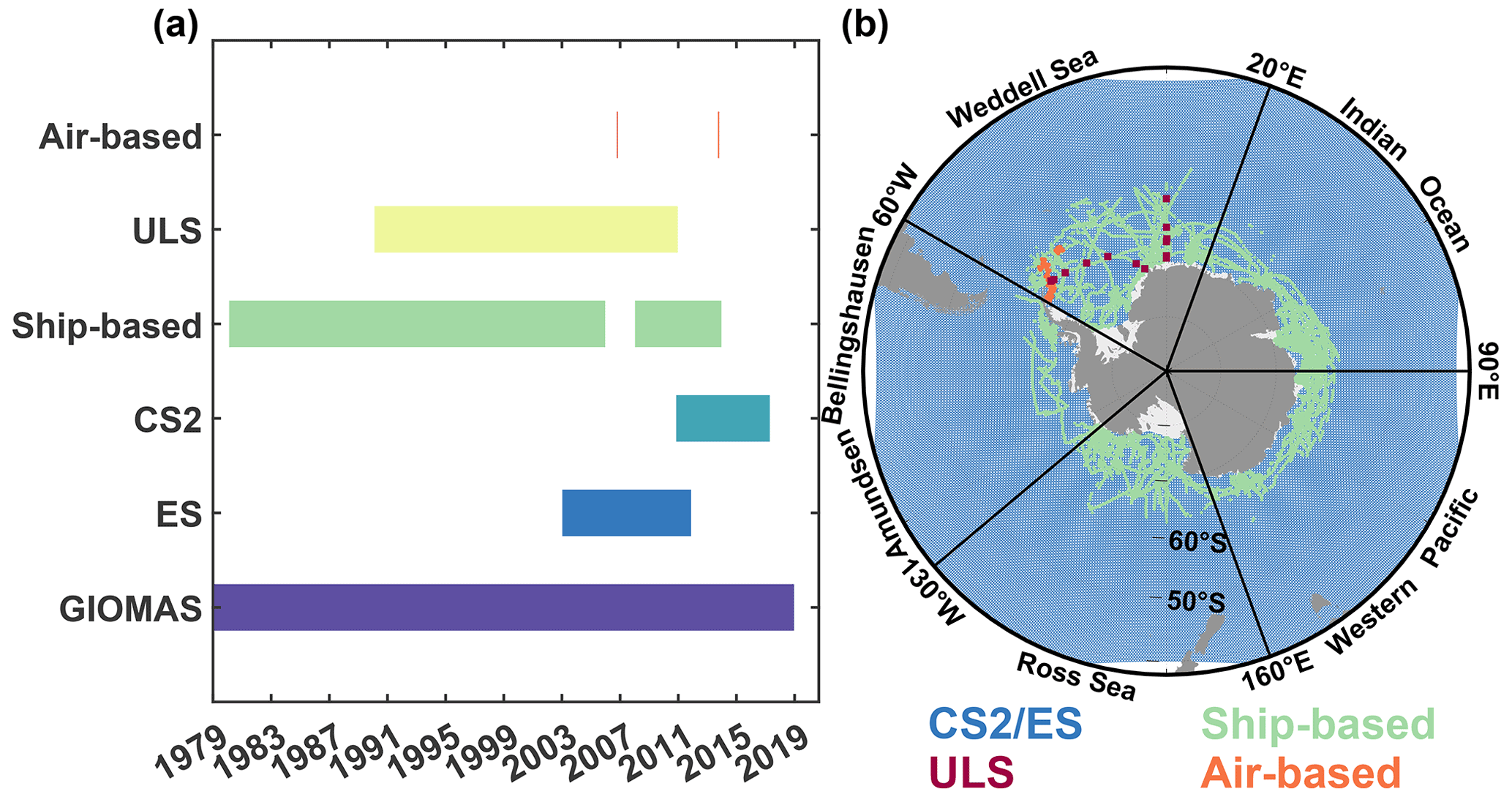
Figure 1 (a) The temporal and (b) spatial coverage of data used in this study.

2.2 SIT from satellite altimeters and in situ observations

Satellite altimeter observations involved in this study are from radar altimeters on board Envisat (ES) and CS2, which are generated by the Sea Ice Climate Change Initiative (SICCI) project under the European Space Agency Climate Change Initiative (ESA CCI) program. ES was equipped with the Radar Altimeter 2, measuring sea-ice freeboard mainly based on the Ku-band frequency (Hendricks et al., 2018b). The Antarctic SIT data derived from ES freeboard span from December 2002 to November 2011 (Fig. 1a) with a coverage of the entire Antarctic (Fig. 1b). The spatial resolution is 50 km × 50 km, and the temporal resolution is 1 month. CS2 was equipped with the SIRAL, measuring the sea-ice freeboard mainly based on the Ku-band frequency like ES (Hendricks et al., 2018a). The CS2 Antarctic SIT dataset spans from November 2010 to April 2017 (Fig. 1a), and the spatial coverage and the spatiotemporal resolution are the same as the ES SIT dataset.

In situ SIT observations involved in this study are from upward-looking sonar (ULS), ship-based and air-based measurements. ULS is a kind of mooring measurement at fixed locations, measuring sea-ice draft (thickness of sea ice below the water surface) with a time interval shorter than 15 min (Behrendt et al., 2013a). Ice draft needs to be converted into total SIT in an empirical way according to Harms et al. (2001). A total of 13 ULSs used in this study were deployed in the Weddell Sea (Fig. 1b) by the Alfred Wegener Institute (AWI) and spanned intermittently from 1990 to 2010 (Fig. 1a).

The ship-based observations are made up of the Antarctic Sea Ice Processes and Climate (ASPeCt) program, ANT-XXIX/6 (Schwegmann, 2013) and ANT-XXIX/7 (Ricker, 2016). The ASPeCt dataset not only includes ASPeCt observations collected from 1981 to 2005 (Worby et al., 2008a) but also the ASPeCt bridge-based sea-ice observations collected from 2007 to 2012. The ship tracks cover all sectors of the Southern Ocean (Fig. 1b), and the average spacing of data points is 6 nmi (11.112 km). The air-based SIT observations include data collected by the air-based electromagnetic system (i.e., like an electromagnetic bird carried by the helicopter) with a high frequency of 0.5 Hz and an average spacing of 3–4 m (Lemke, 2009, 2014, Haas et al., 2011), and they mainly located in the northwest Weddell Sea (Fig. 1b).

Since both satellite observations and in situ observations are involved in the evaluation, it is necessary to investigate the relationship between them. To achieve this, direct comparisons among satellite observations and ULS observations are conducted in the Weddell Sea where ULS SIT observations are available. The monthly SIT of ES and CS2 during their coincident segments (i.e., November 2010 to November 2011) in the Weddell Sea is displayed in Fig. 2a. The SIT of ES and CS2 is mainly distributed around the one-to-one line, and there is a significant correlation of 0.69 between them, indicating ES-derived SIT is comparable to CS2-derived SIT. Then the monthly ES SIT is compared with monthly ULS SIT during the coincident segments at sites 206, 207, 208, 229, 231 and 233 (Fig. 2b). The CS2 dataset is not involved since there are only four data pairs between CS2 and ULS observations. The distribution of data pairs indicates that ES tends to overestimate SIT compared with ULS observations because the scattering surface of the radar altimeter can be inside the snow (Willatt et al., 2010; Wang et al., 2021). However, 77 % of ULS SIT is within the uncertainty of ES (Fig. 2b). Moreover, the correlation between the ULS SIT that is within the uncertainty of ES and the corresponding ES SIT is 0.73. All those indicate that ES-derived SIT is comparable to ULS observations when the uncertainty is considered.

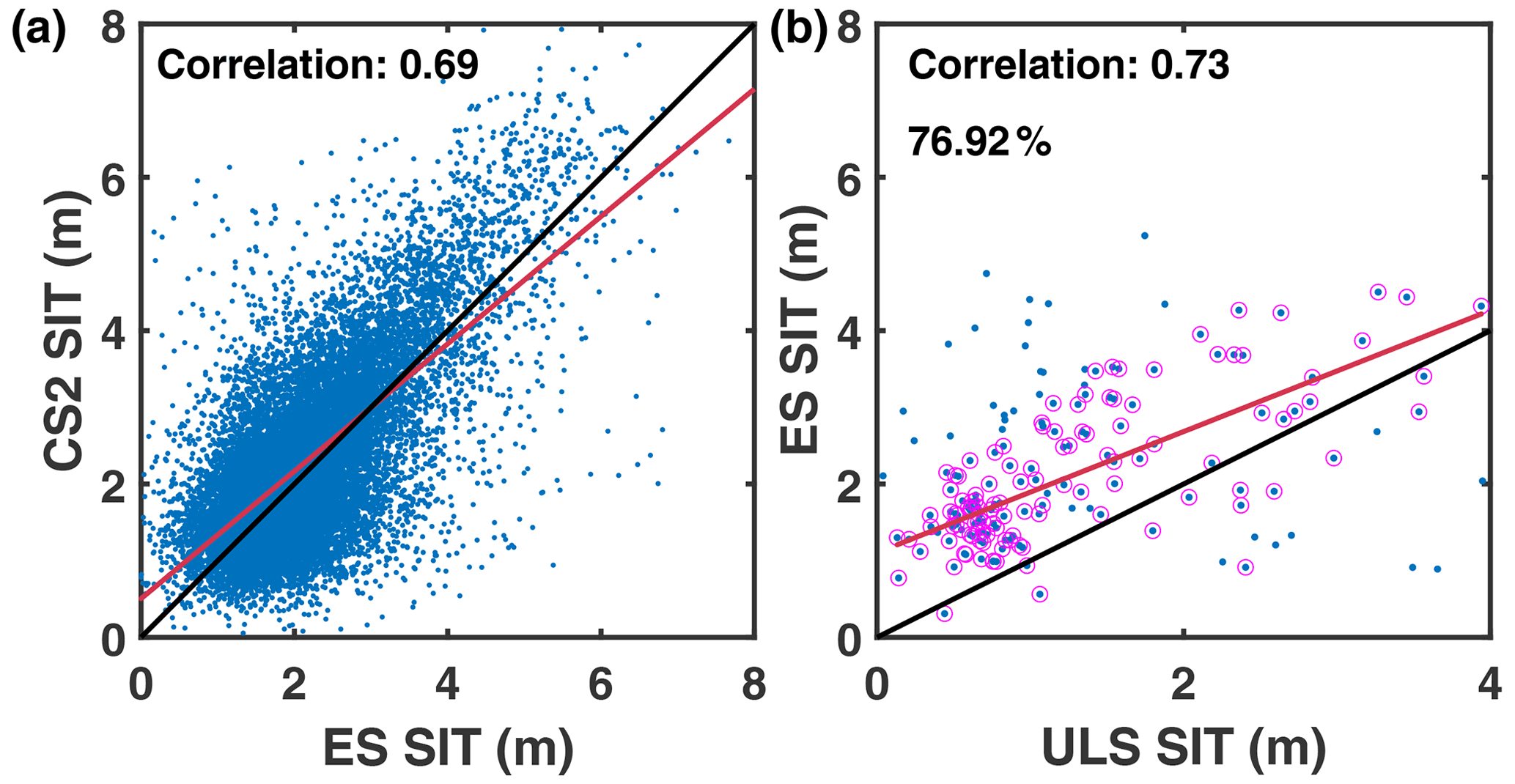
Figure 2 (a) The monthly ES- and CS2-derived SIT in the Weddell Sea during the coincident segment from November 2010 to November 2011 and (b) the monthly ES-derived SIT and ULS observations during the coincident segments at sites 206, 207, 208, 229, 231 and 233. The red lines are linear regression lines, and the black lines are one-to-one lines. The dots surrounded by red circles indicate the ULS SIT is within the uncertainty of ES, and the percentage in (b) denotes the proportion of such dots. The correlation and regression lines in (b) are only for dots surrounded by red circles.

2.3 Data processing and methods

According to Parkinson and Cavalieri (2012), the summer, autumn, winter and spring refer to January–March, April–June, July–September and October–December, respectively. As shown in Fig. 2b, the Southern Ocean is divided into the Weddell Sea (60^∘ W–20^∘ E), the Indian Ocean (20–90^∘ E), the western Pacific Ocean (90–160^∘ E), the Ross Sea (160^∘ E–130^∘ W) and the Amundsen–Bellingshausen Sea (130–60^∘ W).

Since the mismatch in spatial and temporal resolutions between reanalyses and observations could introduce substantial representation errors in the comparisons, the data are processed as Janjić et al. (2018) suggested to eliminate such a mismatch between GIOMAS and observations. In general, GIOMAS data are converted to the locations of the observations when compared with satellite and ULS observations, while the ship-based and air-based observations are converted to gridded data based on the GIOMAS grid. For details, when compared with satellite observations, daily GIOMAS data are interpolated to the grid of satellite observations using the linear approach and converted to monthly averages. For the comparisons between GIOMAS and ULS observations, 15 min ULS data are converted to daily averages for comparison with daily GIOMAS data, and the nearest neighbor approach is used to find the GIOMAS grid cells closest to the ULS locations. Moreover, when compared with ship-based and air-based observations and since the observed data are very dense in space and the temporal resolution is always within 1 d, the data are averaged into daily and gridded data based on the GIOMAS grid to create a proper dataset that is compatible with daily GIOMAS SIT data.

The climatological annual cycle is defined as the multi-year averages in each month. For observations, the climatological annual cycles are calculated from all years available in each observation dataset. For GIOMAS, when compared with satellite observations, GIOMAS data that coincide with the time spans of satellite observations are selected (2002–2011 for ES and 2010–2017 for CS2) to calculate the climatology. When compared with ULS observations, all years available in GIOMAS (1979–2018) are used for the computation of climatology. Anomalies are defined as departures from the climatological annual cycle, and the intensity of variability is defined as the standard deviation of anomalies. During the overlapping time of ES and CS2 (November 2010 to November 2011), though the difference in SIV anomalies between ES and CS2 (i.e., root-mean-square error is 473.1 km³) is not small compared with the mean standard deviation of SIV anomalies (i.e., their standard deviations in ES and CS2 are 960.7 and 956.6 km³, respectively), the selection of data in the coincident segment has little effect on the trend. Thus, the SIV anomalies of CS2 during the overlapping time are chosen, and ES from December 2002 to October 2010 and CS2 from November 2010 to April 2017 are combined to obtain a relatively long and continuous SIV time series for the trend computation. In addition, since the trajectories of air-based SIT observations are mainly distributed in the northwest Weddell Sea, which is dominated by deformed sea ice (Fig. 2b), the comparison between GIOMAS and air-based observations is only conducted in the Weddell Sea.

3 Results

3.1 Comparison in the climatology of SIV and SIT

Figure 3 shows the climatological annual cycle of Antarctic SIV. Although obvious uncertainties in SIV can be found in both ES and CS2, the annual cycle of ES is similar to that of CS2. Both ES and CS2 show that the melt rate of sea ice is nearly twice the growth rate. Moreover, there are also some differences in the SIV climatology between ES and CS2. The SIV of CS2 is greater than that of ES in the winter and spring, and larger uncertainties in SIV can be found in ES. The SIV difference between ES and CS2 may be owing to the mismatch in the sea-ice freeboard between ES and CS2. As Paul et al. (2018) indicated, due to the unresolved physical processes such as complex snow metamorphism or sea-ice surface roughness influenced by the flooding in the snow–ice interface, the sea-ice freeboard of ES cannot be matched well with the ones of CS2 in the Antarctic even though the retracker algorithms are the same. GIOMAS can reproduce the asymmetry in the annual cycle of Antarctic SIV observed by ES and CS2, while it underestimates SIV by about 38 % on average when compared to ES and CS2. Meanwhile, the underestimation is seasonally dependent, with weaker underestimation in summer and stronger in winter.

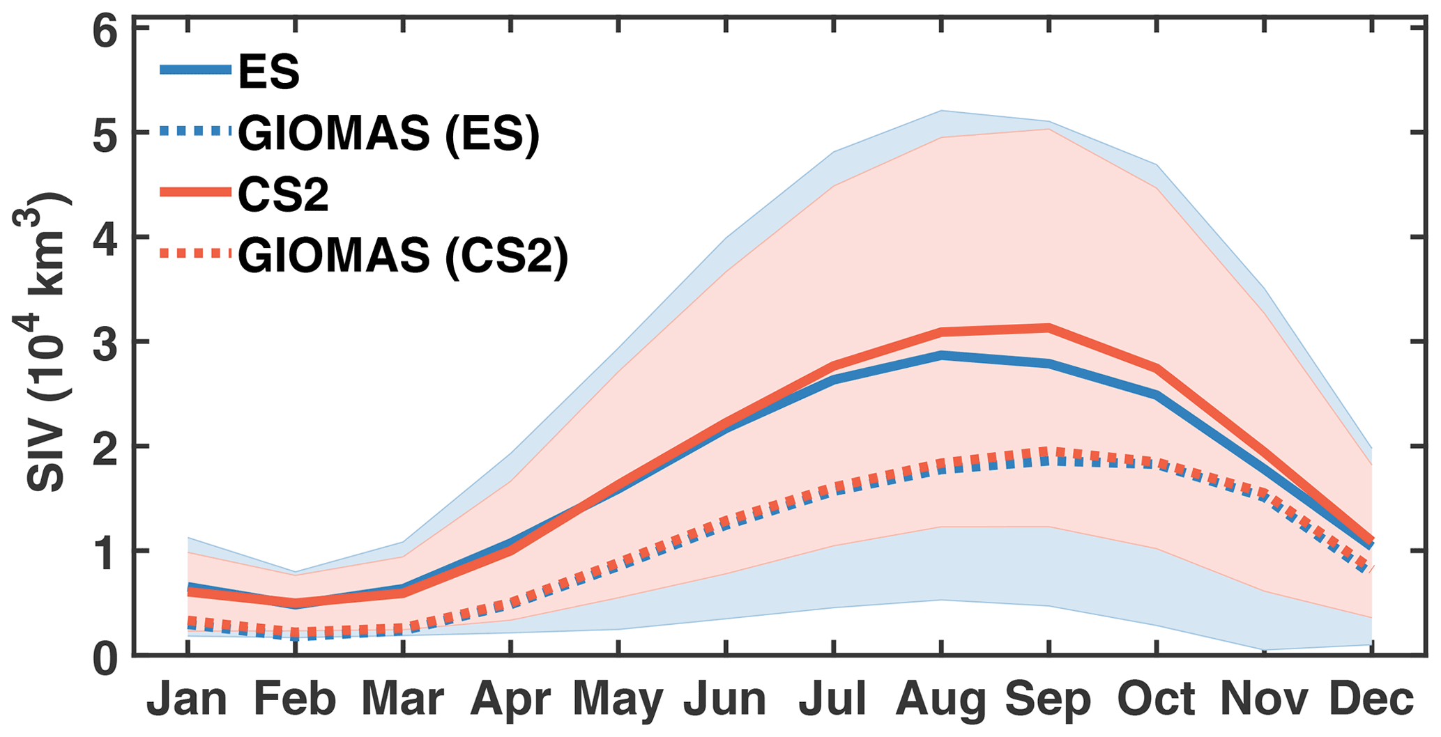
Figure 3 The climatological annual cycle of Antarctic SIV. The blue and red denote data related to ES and CS2, respectively. The solid and dashed curves denote satellite observations and corresponding GIOMAS data. The shaded areas denote the uncertainty of satellite SIV.

Figure 4 shows the spatial distribution of SIT bias in summer and winter to investigate details of SIV underestimation in these two seasons. In both seasons, a significant negative SIT bias of GIOMAS can be found in the deformed ice zone, such as the northwestern Weddell Sea and coasts of the Amundsen–Bellingshausen Sea, as well as the coast of East Antarctica. Meanwhile, the extent of negative bias is wider in the winter (Fig. 4b and d) than in the summer (Fig. 4a and c), which results in seasonal differences in the SIV underestimation (Fig. 3). In addition, there are weakly positive SIT biases in the southwestern Weddell Sea during winter (Fig. 4b and d), which may be due to model bias in simulating sea-ice transport in the western Weddell Sea (Shi et al., 2021). Considering sea-ice deformation is also closely related to sea-ice motion, a better simulation of sea-ice motion is required to achieve a more accurate reconstruction of Antarctic SIT. In addition, the relatively large positive bias in winter Ross Sea SIT can only be found in the comparison between GIOMAS and CS2, which may be caused by the smaller freeboard of CS2 than ES in the winter Ross Sea as shown in Paul et al. (2018). Notably, some of the radar altimeter signals would originate from the snow–air interface or from somewhere inside the snow and result in an overestimation of ice freeboard (Willatt et al., 2010; Wang et al., 2021).

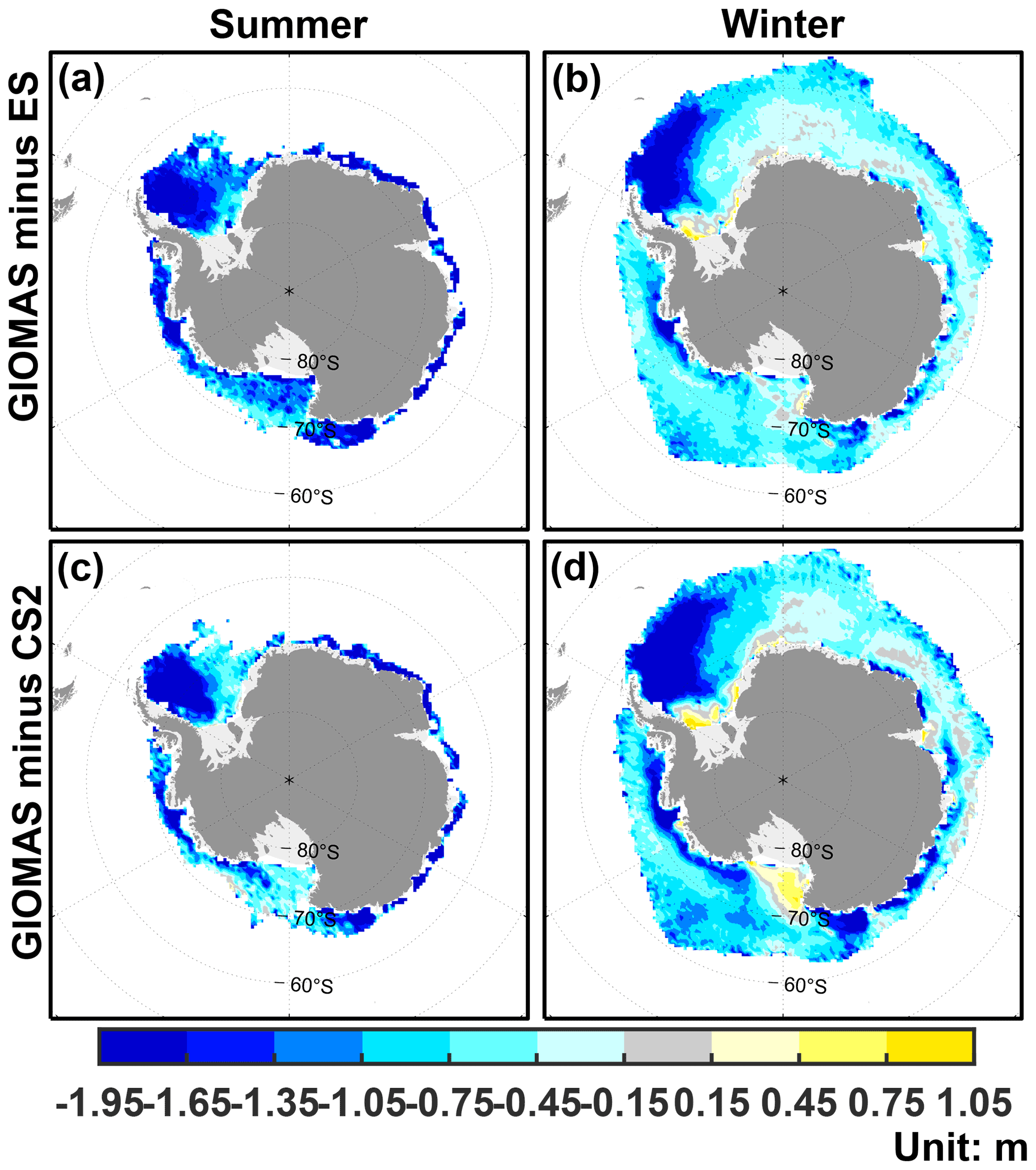
Figure 4 The SIT bias of GIOMAS relative to ES in (a) summer and (b) winter. (c)–(d) Same as (a)–(b) but for bias relative to CS2.

These uncertainties, combined with often thick snow and complex snow metamorphism in the Antarctic, can contribute to the overestimation of the Antarctic SIT from ES and CS2. Thus, the underestimation of SIT from GIOMAS can be partially attributed to the uncertainties in SIT retrieved from ES and CS2. However, the underestimation in the deformed ice regions can be owing to the deficiency of GIOMAS since the differences in SIT between GIOMAS and satellite observations in those regions are always larger than the uncertainties in satellite observations. To prove this, a direct intercomparison between the monthly SIT of GIOMAS, ES and ULS at site 206 is conducted, and the biases of GIOMAS and ES relative to ULS at site 206, and the uncertainties in each dataset are displayed in Table 1. The bias of GIOMAS is larger than the uncertainty of ULS, while the bias of ES is smaller than the uncertainty of ULS (Table 1). This suggests there is a significant discrepancy between GIOMAS and ULS SIT, while ES SIT is comparable to ULS SIT at site 206.

Table 1 The biases of GIOMAS and ES SIT relative to that of ULS and the uncertainties in SIT at ULS 206 (Unit: m).

Due to large uncertainties in the above satellite observations, the SIT of GIOMAS is further assessed by ULS measurement in the Weddell Sea. Considering significant variation in sea ice over horizontal distances as small as a few meters, the standard deviation of ULS is displayed in Fig. 5a. It is obvious that the variability in ULS near the shore (i.e., 206, 207, 212, 217, 232 and 233) is stronger than that of ULS far from the shore (i.e., 208, 209, 210, 227, 229, 230 and 231), indicating larger sea-ice deformation near the shore. As Fig. 5b shows, GIOMAS significantly underestimates the nearshore SIT all year round, while it slightly overestimates SIT far from the shore in the winter, implying the deficiency of GIOMAS in the simulation of sea-ice deformation, which leads to underestimation of SIT in the Weddell Sea from the perspective of regional average. The above deficiency of GIOMAS might be attributed to the insufficient resolutions of the model and assimilated SIC observations, which are not able to resolve the coastal lines well and which hinder GIOMAS from reproducing the ice deformation near the shore. Therefore, GIOMAS is indeed underestimating the climatology of Antarctic SIT, mainly in the deformed sea-ice zone, compared with satellite and in situ observations. In addition to the model drawbacks of GIOMAS, this underestimation might also be introduced by the assimilation procedure of GIOMAS. Although only satellite SIC is nudged in GIOMAS, SIT would be adjusted asymmetrically as described in Sect. 2.1. This asymmetric addition and removal of ice leads to a thinning of the mean ice thickness (Lindsay and Zhang, 2006). Notably, though the uncertainty in satellite observations is large, the differences between GIOMAS and satellite SIT cannot be ignored since the uncertainty in satellite observations is expected to be large owing to the difficulties with the estimation of snow depth and density in the Antarctic (Ozsoy-Cicek et al., 2011; Bunzel et al., 2018).

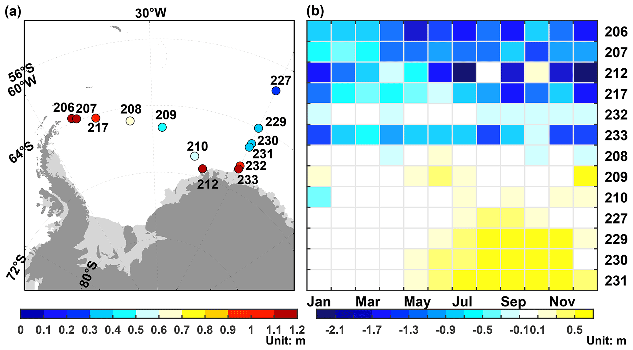
Figure 5 (a) The locations of ULSs in the Weddell Sea and corresponding standard deviation of SIT. (b) The differences in SIT climatology between GIOMAS and ULS.

3.2 Comparison of the trend in SIV

Antarctic SIE shows different trends before and after 2014 (Parkinson, 2019). Though there can be a significant correlation between Antarctic SIE and SIV, differences between the variation in SIV and SIE cannot be ignored in some regions. Therefore, it is necessary to examine whether there are similar changes in the trend in Antarctic SIV. As Fig. 6 shows, the observed Antarctic SIV anomaly increased gradually from 2003 onwards, reached the maximum (2783 km³) in November 2013 and then abruptly declined from September 2013 to April 2017. The evolution of the SIV anomaly is comparable to that of the SIE anomaly, while the time of the SIV anomaly peak is earlier than that of the SIE anomaly peak by nearly 1 year. The trends in GIOMAS and observed SIV anomalies are 989 and 2968 km³ per month before 2013 and −84 762 and −119 875 km³ per month after 2013. Although there are differences in the SIV trend between GIOMAS and satellite observation, GIOMAS can basically reproduce the changes in the observed SIV trend before and after 2013. Moreover, the correlation of SIV anomalies between GIOMAS and observations is 0.83, which passes a two-tailed t test at 99 % significance level. Given the advantages of reanalyses over observations or models individually especially in the polar region (Buehner et al., 2017), GIOMAS data would be a good choice to study the variability and long-term trends in Antarctic sea ice.

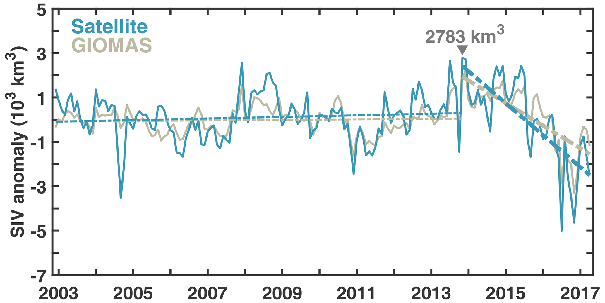
Figure 6 The SIV anomalies of satellite (green) and corresponding GIOMAS (khaki) observations. The dashed lines denote the linear trends in SIV anomalies from December 2002 to November 2013 and from November 2013 to April 2017. The bold dashed lines indicate that the linear trends have passed an F test at 99 % significance level.

3.3 Comparison in the intensity of SIT variability

Figure 7 displays spatial differences in the intensity of SIT anomaly variability between GIOMAS and satellite observations. Compared with ES and CS2, GIOMAS underestimates the intensity of SIT variability in the Southern Ocean, especially in the deformed ice zone (Fig. 7a–b), which resembles the spatial pattern of Fig. 4. The underestimation in the deformed ice regions can be found also in the comparison between GIOMAS and ULS. The intensity of SIT variability is underestimated near the shore, while it is overestimated away from the shore (Fig. 7c). The spatial distribution of differences in the intensity of variability is roughly consistent with that of SIT differences in Fig. 5b. These phenomena suggest that there appears to be a relationship between the mean SIT and the variability. As Blanchard-Wrigglesworth and Bitz (2014) suggested, models with a thinner mean ice state tend to have SIT anomalies with smaller amplitude. In addition, the comparison of SIT standard deviation ratio and mean bias between GIOMAS and satellite observations shown in the Supplement further clarifies the relationship that with a negative SIT bias, GIOMAS always underestimates the variability in SIT. Thus, the bias of SIT has an impact not only on the climatology of SIT but also on the variability in SIT. It should be mentioned that in the regions where the uncertainty in satellite observations is larger than the difference between GIOMAS and satellite observations (i.e., mainly in the regions with undeformed sea ice), the uncertainty would have an impact on the evaluation of the variability in SIT and cannot be ignored.

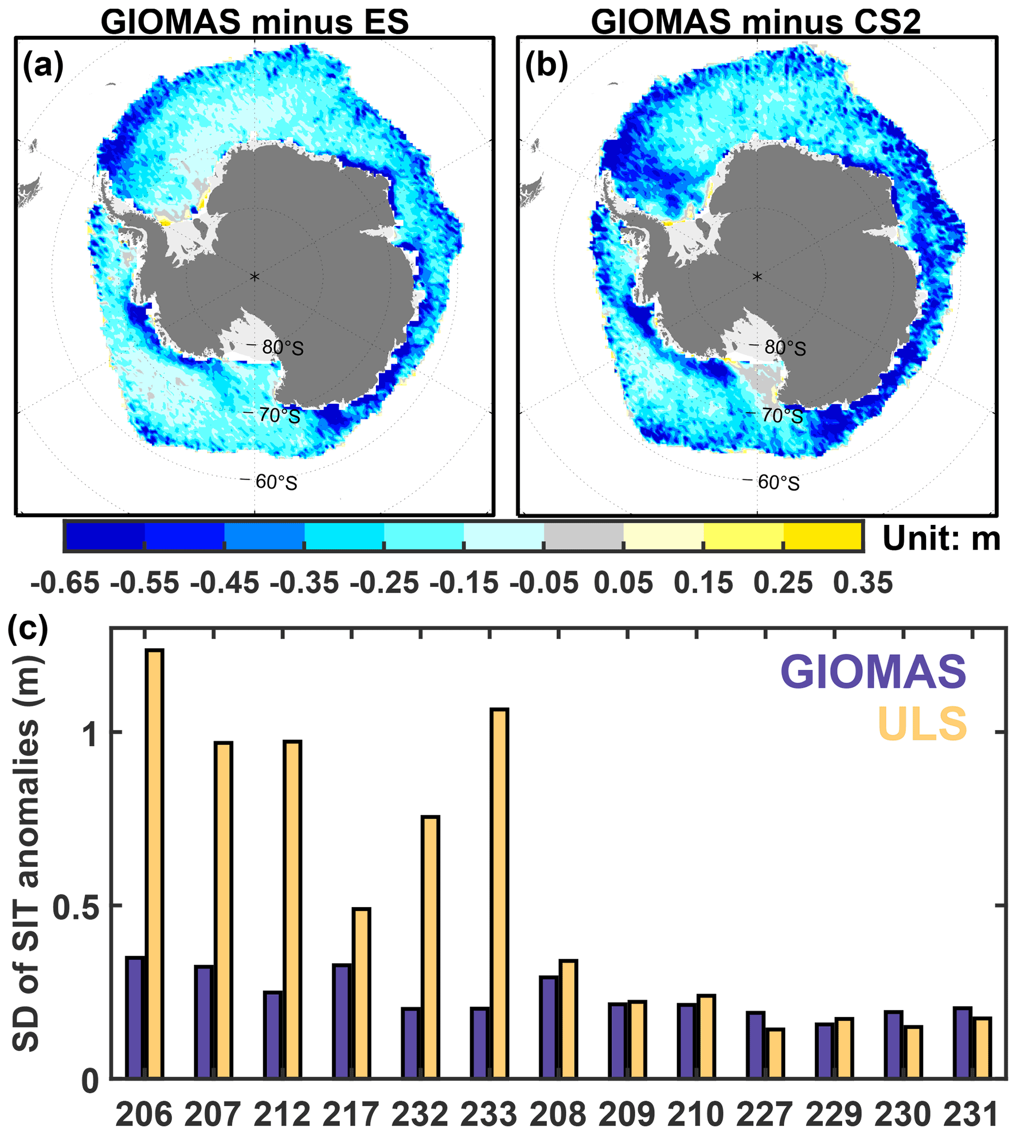
Figure 7 (a) The spatial differences in standard deviation of SIT anomalies between GIOMAS and ES. (b) Same as (a) but for differences between GIOMAS and CS2. (c) The standard deviation of SIT anomalies for ULS (yellow) and corresponding GIOMAS (blue).

3.4 Comparison of SIT frequency

In addition to ULS observations, the rest of the in situ sea-ice observations are sparse in the Southern Ocean and are mainly provided by ship-based and air-based measurements. Figure 8 displays the SIT frequency distribution of GIOMAS and ship-based and air-based in situ observations. The peaks of observations are mainly around 0–0.6 m, while the frequencies of GIOMAS SIT are mainly distributed in the 0–1.4 m depths in the Southern Ocean (Fig. 8a). In different sectors (Fig. 8b–f), the frequency distribution of observed SIT data is similar to that in the whole Southern Ocean, while the peaks of GIOMAS SIT frequency vary from 0.2 to 1.4 m. Compared with observations, for the Southern Ocean, GIOMAS has a higher frequency within 0.6–1.6 m, while it has a lower frequency in the rest of the bins compared with ship-based observations (Fig. 8a), which seems to imply the overestimation of SIT. Similar results can be found in different sectors (Fig. 8b–f). However, the sample selection bias should be noted in the ship-based observations due to a ship's track avoiding areas of thicker ice, which results in its estimation biased toward thinner ice (Timmermann, 2004; Williams et al., 2015). Moreover, GIOMAS has a lower frequency of thick ice in the Weddell Sea compared with air-based observations. In conclusion, GIOMAS tends to overestimate SIT frequency between 0.6 and 1.6 m in the Southern Ocean compared with ship-based observations under the premise that ship-based observations always bias low. Additionally, the comparison between GIOMAS and air-based SIT observations further proves the weakness of GIOMAS in the simulation of sea-ice deformation.

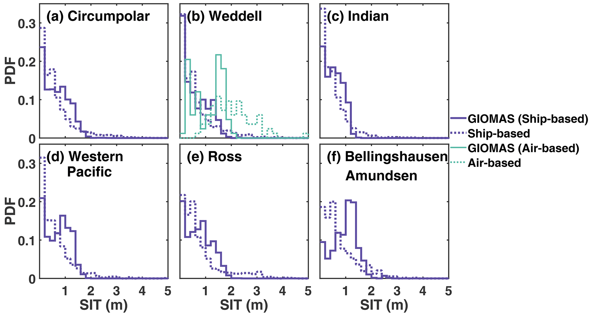
Figure 8 SIT histograms of GIOMAS and in situ observations in (a) the Southern Ocean and (b–f) different sectors.

4 Conclusions and discussion

Considering the important role of SIT in studies of Antarctic sea ice and the wide application of GIOMAS, the Antarctic SIT of GIOMAS is assessed with satellite and in situ observations. In general, GIOMAS can basically reproduce the observed variability and linear trends in SIV even though only satellite SIC data are assimilated by nudging. For the climatology, GIOMAS can reproduce the asymmetry in the annual cycle of Antarctic SIV. For the long-term SIV variation, the variation in GIOMAS is in phase with that of observations, and it is also able to capture the changes in linear trends before and after 2013. These suggest that GIOMAS is useful to study the long-term variation in Antarctic sea ice. However, significant negative bias in SIT can be found in the comparison between GIOMAS and observations. Compared with satellite measurements, GIOMAS tends to underestimate SIT, especially in regions with strong ice deformation. This underestimation is of seasonal dependence with greater underestimation in the winter. Although the above underestimation can be partially attributed to the uncertainties in SIT retrieved from a satellite especially in the undeformed ice zone, the differences cannot be ignored, and SIT underestimation in the northwest Weddell Sea is further verified by the comparison between GIOMAS and ULS observations. Furthermore, the spatial distribution of the differences in the magnitude of SIT variability resembles that of the differences in SIT climatology between GIOMAS and observations. Given the relationship between mean state of SIT and variability (Blanchard-Wrigglesworth and Bitz, 2014; also verified by the comparison between satellite observations and GIOMAS in the Supplement), this phenomenon indicates that SIT underestimation might have an impact on not only the SIT climatology but also the SIT variability. In addition, GIOMAS overestimates SIT compared with ship-based observations, which can be due to the negative bias in ship-based SIT estimation (Timmermann, 2004; Williams et al., 2015). The deficiency of GIOMAS in simulating deformed sea ice is further verified in the comparison with air-based observations.

Notably, though GIOMAS could basically reproduce the trends in Antarctic SIV anomalies before and after 2013, the differences in the trends in SIV anomalies between GIOMAS and satellite observations cannot be ignored. A simple comparison between the monthly GIOMAS sea-surface temperature (SST) and microwave optimally interpolated SST observations reveals that the positive bias of GIOMAS in SST before 2014 roughly corresponds to the underestimation of positive trends in observed SIV anomalies, while the negative SST bias of GIOMAS after 2014 corresponds to the underestimation of negative trends in observed SIV anomalies. There seems to be a possible relationship between the difference in SST and the difference in the trends in SIV anomalies between GIOMAS and observations since higher SST would slow down the increase in SIV, while lower SST would slow down the decrease in SIV. However, this relationship needs further quantification, and further analysis is added to our future work plan.

In addition, limitations of Antarctic SIT observations are non-negligible in this study. For one aspect, the scarcity of Antarctic SIT observations is one of the main sources of limitations for the evaluation. The time span of satellite observations is not long enough for the evaluation of GIOMAS SIT data from 1979 to the present, while the in situ observations are too few to show the estimation of SIT in the entire Southern Ocean. Those prevent the comprehensive evaluation of the entire GIOMAS Antarctic SIT data in this study. For another, this study is also limited by observations of Antarctic SIT due to their unsuitability for the evaluation. For example, though SIT from ICESat (Kern et al., 2016) equipped with the Geoscience Laser Altimeter System is available from 2004 to 2008 and has been proven to have lower bias in SIT estimation than radar altimeter measurements (Willatt et al., 2010; Wang et al., 2021), it is not adopted in this study. The reasons are as follows. First, ICESat SIT is not available in winter (July–September), when greater underestimation of SIT is found in GIOMAS (Fig. 3). Second, the data size of ICESat is relatively smaller than that of ES and CS2 because ICESat provides seasonal mean data, and its time range is narrower. Therefore, the additional assessment on the SIT of GIOMAS will be conducted when the Antarctic SIT derived from ICESat-2 is available. Furthermore, the uncertainty in satellite observations has an impact on the evaluation and the accuracy of satellite observations and needs to be further improved to obtain more accurate satellite-derived SIT estimations with smaller uncertainty. The uncertainty in satellite-derived SIT observations is mainly from the uncertainty introduced by the scattering surface of radar signals and the estimation of Antarctic snow depth and density. With the influences of complex snow stratigraphy and flooding inside the snow related to the formation of snow ice, the assumption that the radar signal is reflected from the snow–ice interface is not applicable in most cases (Willatt et al., 2010). Moreover, owing to the lack of knowledge of Antarctic snow, the climatology of snow depth from the European Space Agency SICCI Advanced Microwave Scanning Radiometer for the Earth Observing System (AMSR-E) and the Advanced Microwave Scanning Radiometer 2 (AMSR2) is used in the retrieval of ES- and CS2-derived SIT, which would introduce extra uncertainties since the interannual variability in snow depth is omitted (Bunzel et al., 2018). Moreover, AMSR-E and AMSR2 have been shown to considerably underestimate the actual snow depth, which usually occurs in the East Antarctic (Worby et al., 2008b; Ozsoy-Cicek et al., 2011). All those contribute to the large uncertainty in the satellite-derived SIT in the Antarctic, and the uncertainty would influence the evaluation of SIT in the regions where the differences between GIOMAS SIT and satellite observations are smaller than the uncertainty. Therefore, a more accurate estimation of Antarctic snow depth and density would be essential in reducing the uncertainty in satellite SIT observations and thus improving the reliability of the evaluation.

The above SIT underestimation of GIOMAS can be partially attributed to the model weakness. For example, insufficient resolution of the model restricts GIOMAS to reproduce the ice deformation near the shore. Moreover, the assimilation is a vital component in the reanalyses since it could constrain the model with observations and make the model obtain a better state estimation (Lahoz and Schneider, 2014). However, it can also be a source of errors in the system. In GIOMAS, the asymmetric SIT changes introduced by assimilation cannot be ignored. Thus, besides the further development of the model, there are potential ways to improve the estimation of Antarctic SIT from the perspective of data assimilation. Firstly, additional sea-ice observations other than SIC should be assimilated. For example, besides Antarctic SIT derived from Envisat and CryoSat-2 used in this study, the Antarctic SIT retrieved from ICESat-2 is also to be released in the near future, and hence assimilating these SIT observations directly may suppress the bias of SIT (e.g., Yang et al., 2014; Fritzner et al., 2019; Luo et al., 2021). Also, assimilating sea-ice drift observations can improve the simulation of sea-ice motion and deformation, which can improve the estimation of SIT (e.g., Lindsay and Zhang, 2006; Mu et al., 2020). Secondly, advanced data assimilation methods should be adopted to provide balanced estimation of model state. For instance, the innovation of SIC can be converted to the increment of SIT in a more balanced way through the flow-dependent covariance of the ensemble Kalman filter (e.g., Massonnet et al., 2013; Yang et al., 2015). Thirdly, due to the characteristics of SIC observations derived from the passive microwave instrument, observation errors of SIC should vary with time and location (Lindsay and Zhang, 2006). However, a fixed value of observation errors is adopted in GIOMAS because of limited information on observation errors of SIC. Thus, a better estimation of SIC observation errors might further improve the performance of GIOMAS. Furthermore, though nudging of SIC is not state of the art, it makes the model of GIOMAS obtain a better SIT simulation, while the model-only data of GIOMAS are likely to overestimate SIT in the marginal seas. To promote the development of GIOMAS, further quantitative analyses on the impact of nudging SIC on the SIT in the Antarctic are worthy of attention and will be conducted in the future.

Moreover, in the course of global warming, Antarctic SIE rose gradually and reached a record high in 2014/2015 before decreasing dramatically, which is obviously different from the dramatic drop in Arctic SIE during the satellite era (e.g., Turner and Comiso, 2017). Results from a recent study suggest that the trend in Antarctic ice coverage may be due to changes in atmospheric (e.g., Holland and Kwok, 2012) and oceanic (e.g., Meehl et al., 2019) processes. Without better SIT and SIV estimates, it is difficult to characterize how Antarctic sea-ice cover is responding to changing climate or which climate parameters are most influential (Vaughan et al., 2013). Thus, more Antarctic sea-ice observations and more studies on data assimilation are urgently needed to accurately evaluate the Antarctic SIT, which can help to improve the reconstruction and prediction of Antarctic SIV and to support research related to Antarctic sea ice.