the Creative Commons Attribution 4.0 License.
the Creative Commons Attribution 4.0 License.
 | 05 May 2022
Network connectivity between the winter Arctic Oscillation and summer sea ice in CMIP6 models and observations
William Gregory
Julienne Stroeve
Michel Tsamados
The indirect effect of winter Arctic Oscillation (AO) events on the following summer Arctic sea ice extent suggests an inherent winter-to-summer mechanism for sea ice predictability. On the other hand, operational regional summer sea ice forecasts in a large number of coupled climate models show a considerable drop in predictive skill for forecasts initialised prior to the date of melt onset in spring, suggesting that some drivers of sea ice variability on longer timescales may not be well represented in these models. To this end, we introduce an unsupervised learning approach based on cluster analysis and complex networks to establish how well the latest generation of coupled climate models participating in phase 6 of the World Climate Research Programme Coupled Model Intercomparison Project (CMIP6) are able to reflect the spatio-temporal patterns of variability in Northern Hemisphere winter sea-level pressure and Arctic summer sea ice concentration over the period 1979–2020, relative to ERA5 atmospheric reanalysis and satellite-derived sea ice observations, respectively. Two specific global metrics are introduced as ways to compare patterns of variability between models and observations/reanalysis: the adjusted Rand index – a method for comparing spatial patterns of variability – and a network distance metric – a method for comparing the degree of connectivity between two geographic regions. We find that CMIP6 models generally reflect the spatial pattern of variability in the AO relatively well, although they overestimate the magnitude of sea-level pressure variability over the north-western Pacific Ocean and underestimate the variability over northern Africa and southern Europe. They also underestimate the importance of regions such as the Beaufort, East Siberian, and Laptev seas in explaining pan-Arctic summer sea ice area variability, which we hypothesise is due to regional biases in sea ice thickness. Finally, observations show that historically, winter AO events (negatively) covary strongly with summer sea ice concentration in the eastern Pacific sector of the Arctic, although now under a thinning ice regime, both the eastern and western Pacific sectors exhibit similar behaviour. CMIP6 models however do not show this transition on average, which may hinder their ability to make skilful seasonal to inter-annual predictions of summer sea ice.
- Article
(12879 KB) - Full-text XML
-
Supplement
(9539 KB) - BibTeX
- EndNote


Arctic sea ice is a key component of the polar climate system, acting as a barrier which both reflects incoming solar radiation and regulates the rate of energy exchange between the atmosphere and ocean. Over the past four decades, however, it can be seen as a direct barometer for climate change, having suffered significant losses in areal extent across all seasons (Stroeve and Notz, 2018), linked to the long-term increase in anthropogenic CO2 emissions (Notz and Stroeve, 2016). Such sea ice decline has profound implications for regional Northern Hemisphere circulation patterns (Francis et al., 2009; Cohen et al., 2014, 2020), ecological productivity (Sakshaug et al., 1994; Stirling, 1997; Stroeve et al., 2021), and coastal communities (Fritz et al., 2017; Larsen et al., 2021) in present and future decades, as many model studies now predict the increasing likelihood of a seasonally ice-free Arctic Ocean occurring before the middle of this century (Stroeve et al., 2007; Jahn, 2018; Notz and SIMIP-Community, 2020; Årthun et al., 2021). Imprinted on this observed sea ice decline is a pattern of significant inter-annual variability, particularly in the summer months (e.g. Onarheim et al., 2018; Stroeve and Notz, 2018). Subsequently, understanding the drivers of such variability has important consequences for our ability to make reliable sea ice predictions on seasonal to inter-annual timescales. A number of studies, for example, have highlighted various climatological teleconnections as key drivers of sea ice variability, including land–ice (typically via the atmosphere; Serreze et al., 1995; Overland et al., 2012; Matsumura et al., 2014; Crawford et al., 2018), atmosphere–ice (Deser et al., 2000; Kapsch et al., 2013; Park et al., 2018; Olonscheck et al., 2019), ocean-ice (Venegas and Mysak, 2000; Vinje, 2001; Zhang, 2015), and ice–ice interactions (Schröder et al., 2014; Bushuk and Giannakis, 2017), suggesting inherent sources of sea ice predictability across the various components of the climate system. Furthermore, coupled climate models have demonstrated a horizon of sea ice predictability beyond 12 months lead time based on so-called “perfect-model” experiments (Holland et al., 2011; Tietsche et al., 2014; Day et al., 2014; Bushuk et al., 2019). Operationally, however, regional summer sea ice forecasts (in models) appear to be strongly controlled by a “spring predictability barrier” (Bonan et al., 2019) which is governed by the date of melt onset in the preceding spring (Bushuk et al., 2020). This leads to the question as to how well climate models reflect the teleconnections known to drive summer sea ice variability given the gap between perfect-model and operational regional forecast skill in those models (Bushuk et al., 2019). Recent work has gone into investigating physically based mechanisms for sea ice predictability (Bushuk and Giannakis, 2017; Bonan and Blanchard-Wrigglesworth, 2020; Giesse et al., 2021) in order to assess whether the shortfalls in operational climate model forecasts can, in part, be attributed to lack of representation of such mechanisms across a wide range of general circulation models (GCMs). In this study we pursue a similar line of investigation, looking specifically at the Arctic Oscillation (AO) teleconnection (Thompson and Wallace, 1998), whose winter pattern has been shown to explain up to 22 % of the variability in pan-Arctic September sea ice extent (Park et al., 2018). Historically, the dominant spatio-temporal modes of winter sea-level pressure variability have been somewhat misrepresented in the majority of GCMs participating in previous phases of the Coupled Model Intercomparison Project (CMIP), e.g. CMIP3 (Miller et al., 2006; Cattiaux and Cassou, 2013) and CMIP5 (Zuo et al., 2013; Gong et al., 2016), which naturally has implications for the representation of the AO to sea ice teleconnection in those models. Here, we assess the spatio-temporal patterns of variability in both winter sea-level pressure and summer sea ice concentration and also the presence of the winter AO to summer sea ice teleconnection over the period 1979–2020 in the latest generation of GCMs submitted to CMIP6 (Eyring et al., 2016) and how this teleconnection may be changing over time as the ice cover thins and is more susceptible to atmospheric forcing (Maslanik et al., 1996; Mioduszewski et al., 2019). Similar to previous works (Fountalis et al., 2014, 2015; Gregory et al., 2020), our method here is based on complex networks, an approach which provides a relatively simple and visual framework with which to analyse and display large volumes of data that typically represent complex physical systems. Their use across multiple disciplines has grown considerably over recent decades, with intuitive applications in computer science and social networks (Albert and Barabási, 2002; Newman, 2003; Boccaletti et al., 2006; Cohen and Havlin, 2010) – known as structural networks – to more abstract applications in, for example, neuroscience (Zhou et al., 2007; Morabito et al., 2015; delEtoile and Adeli, 2017), seismology (Abe and Suzuki, 2006), and climate science (Tsonis and Roebber, 2004; Tsonis et al., 2006; Donges et al., 2009; Fountalis et al., 2014; Dijkstra et al., 2019; Gregory et al., 2020) – known as functional networks. Climate network analysis was first introduced by Tsonis and Roebber (2004) and has subsequently proven to be a powerful tool kit for extracting statistical information from the array of climatological teleconnections that govern climate variability and is a useful addition to more conventional approaches of analysing spatio-temporal patterns of variability, such as empirical orthogonal function (EOF) analysis (Donges et al., 2015). Our motivation for choosing the networks approach here is two-fold. For one, complex networks have become increasingly popular over the past decade as a way to analyse large-scale teleconnections in climate science (as detailed in the references above); however their application in the polar domains has been somewhat limited. On the other hand, the networks approach does also provide some specific advantages over traditional EOF analysis. Specifically, EOF analysis is variance greedy, whereby each mode represents the direction along which the variance of the data is largest, and so patterns of lower variance are inherently masked. Furthermore orthogonality constraints restrict each mode to an orientation that is orthogonal to all other modes. In contrast, the networks approach has neither of these constraints and in addition provides an initial framework which can be modified with relative ease to incorporate a variety of principles ranging from non-linear associations (Donges et al., 2009; Malik et al., 2012; Boers et al., 2014) to causal inference (Runge et al., 2019). This paper is structured as follows: in Sect. 2 we introduce the sea ice observations, atmospheric reanalysis, and CMIP6 model data that are used to generate complex networks of the respective sea ice and atmospheric fields. In Sect. 3 we introduce the complex networks methodology and two global metrics which are used to describe similarities and differences between networks. In Sect. 4 we present the results of the networks generated from CMIP6 model outputs and discuss their similarities and differences relative to the observations and reanalysis data, and furthermore we evaluate the presence of the winter AO to summer sea ice teleconnection across all models. We then end with a discussion and conclusions in Sect. 5.
2.1 Observations
For analysing summer sea ice concentration variability in the observations, we compute the average of monthly mean June, July, August, and September (JJAS) sea ice concentration fields between 1979 and 2020 from three separate observational data sets based on the series of multi-frequency passive microwave satellite observations since October 1978. These include the National Snow and Ice Data Center (NSIDC) NASA Team (Cavalieri et al., 1996) and Bootstrap (Comiso, 2017) products, as well as the Ocean and Sea Ice Satellite Application Facility (OSI-SAF) OSI-450 (1979–2015) and OSI-430-b (2016–2020) products (OSI-SAF, 2017; Lavergne et al., 2019). We use three different products as each has subtle variations in their summer variability, i.e. how each account for new melt-pond formation (Comiso et al., 2017). Each of the three data sets apply separate processing algorithms to passive microwave brightness temperatures derived from multiple satellites across the historical record: Nimbus-7 SMMR (1979–1987), the DMSP F-8, F-11, and F-13 SSM/Is (1987–2007), and finally the DMSP F-18 SSM/I (2007–2020). These data are provided on 25 km × 25 km polar stereographic (NASA Team and Bootstrap) and EASE (OSI-450 and OSI-430-b) grids, which are re-gridded to a common 50 km × 50 km polar stereographic grid using a nearest neighbour interpolation here for computational reasons. Grid cell area information (used to generate area-weighted time series, see Sect. 3.1) was also extracted from NSIDC's pixel area tools library.
2.2 Atmospheric reanalysis
The AO is typically defined as the leading mode of variability in mean sea-level pressure data north of 20∘ N (Thompson and Wallace, 1998). As a proxy for an observational record of the winter AO here, we compute the average of monthly mean December, January, February, and March (DJFM) mean sea-level pressure data north of 20∘ N from ERA5 reanalysis (Hersbach et al., 2019). We only use one reanalysis product due to the high consistency of sea-level pressure fields between different reanalyses over the Arctic region (Graham et al., 2019). As December data are not available for the year 1978 for ERA5, the winter period in 1979 corresponds to the average of January, February, and March data. Sea-level pressure fields are output on a latitude–longitude grid. In Sect. 5 we also make use of the Pan-Arctic Ice Ocean Modeling and Assimilation System (PIOMAS) sea ice thickness model (Zhang and Rothrock, 2003) to help explain some of the features related to the winter AO to summer sea ice teleconnection. PIOMAS is a coupled ice–ocean model that assimilates observed sea ice concentration and sea surface temperatures (open water only) and is forced by NCEP-NCAR (National Centers for Environmental Prediction and National Center for Atmospheric Research) atmospheric reanalysis. Although it is a model, it has been shown to be relatively consistent with in situ and submarine observations (Schweiger et al., 2011) and generally has consistent biases with CMIP3 and 5 models relative to observational data in terms of its ice thickness distribution (Stroeve et al., 2014). Furthermore, it is able to provide consistent coverage over the observational period.
2.3 CMIP6 model outputs
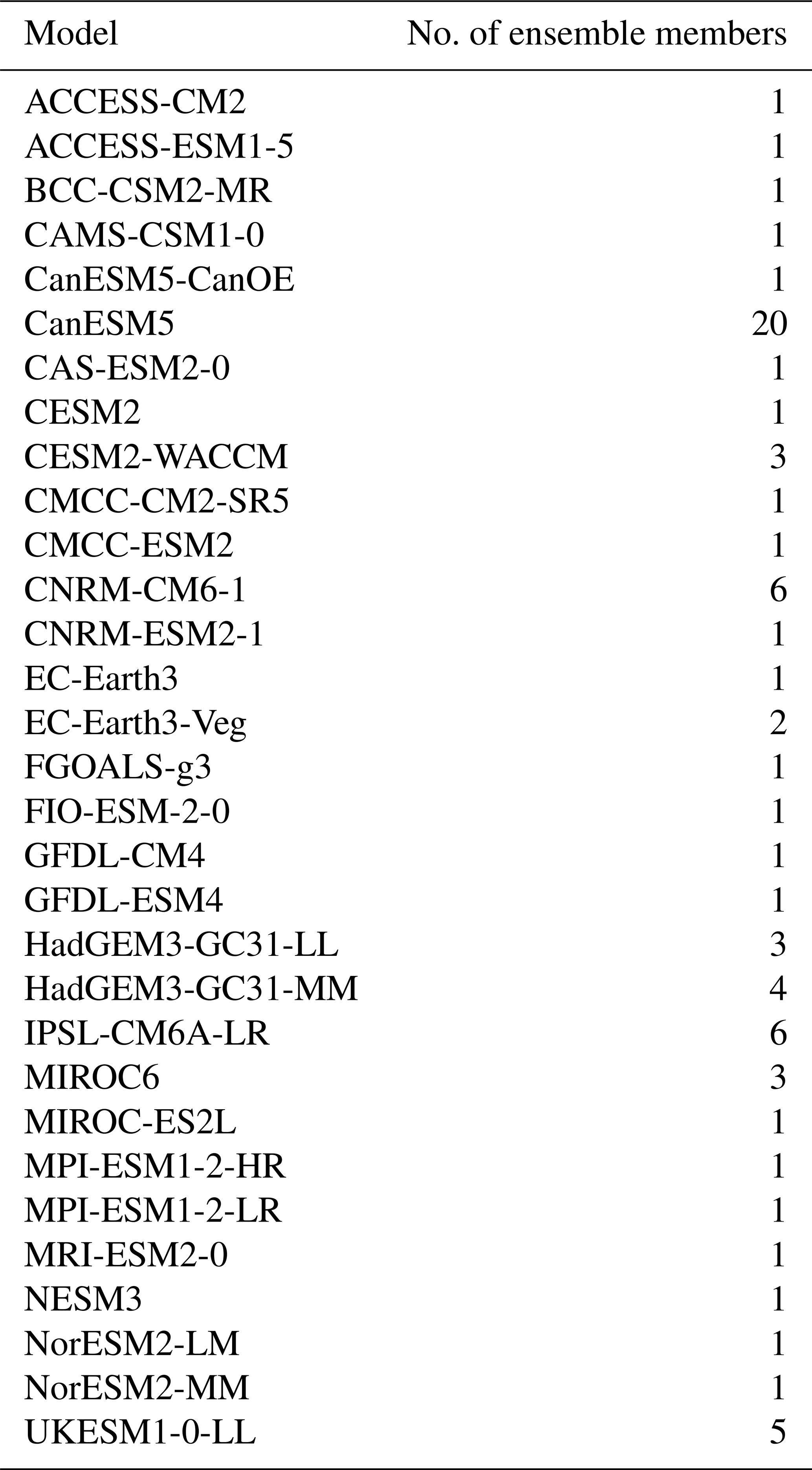
We assess the seasonal patterns of variability in sea ice concentration and mean sea-level pressure outputs from 31 different GCMs participating in CMIP6. In order to compare with recent observations, we combine monthly averaged model outputs from historical runs (1979–2014) with ScenarioMIP run SSP5-8.5 (Gidden et al., 2019) to extend the analysis period to 2020; hence only model ensemble members which contain historical and ScenarioMIP outputs for both sea ice concentration and mean sea-level pressure are considered in this work. As detailed above, we compute the corresponding winter (DJFM) and summer (JJAS) averages for mean sea-level pressure and sea ice concentration outputs, respectively. Sea ice concentration outputs are also re-gridded to the same 50 km × 50 km polar stereographic grid as the observational data sets, and mean sea-level pressure outputs are re-gridded to a latitude–longitude grid. The chosen models, along with their respective number of available ensemble members, are summarised in Table 1.
3.1 Complex networks
Generating complex networks here follows the methodology from previous studies (Fountalis et al., 2014; Gregory et al., 2020). In this section we summarise the key steps and present an example DJFM sea-level pressure network from ERA5, as well as JJAS sea ice concentration networks from the observations.
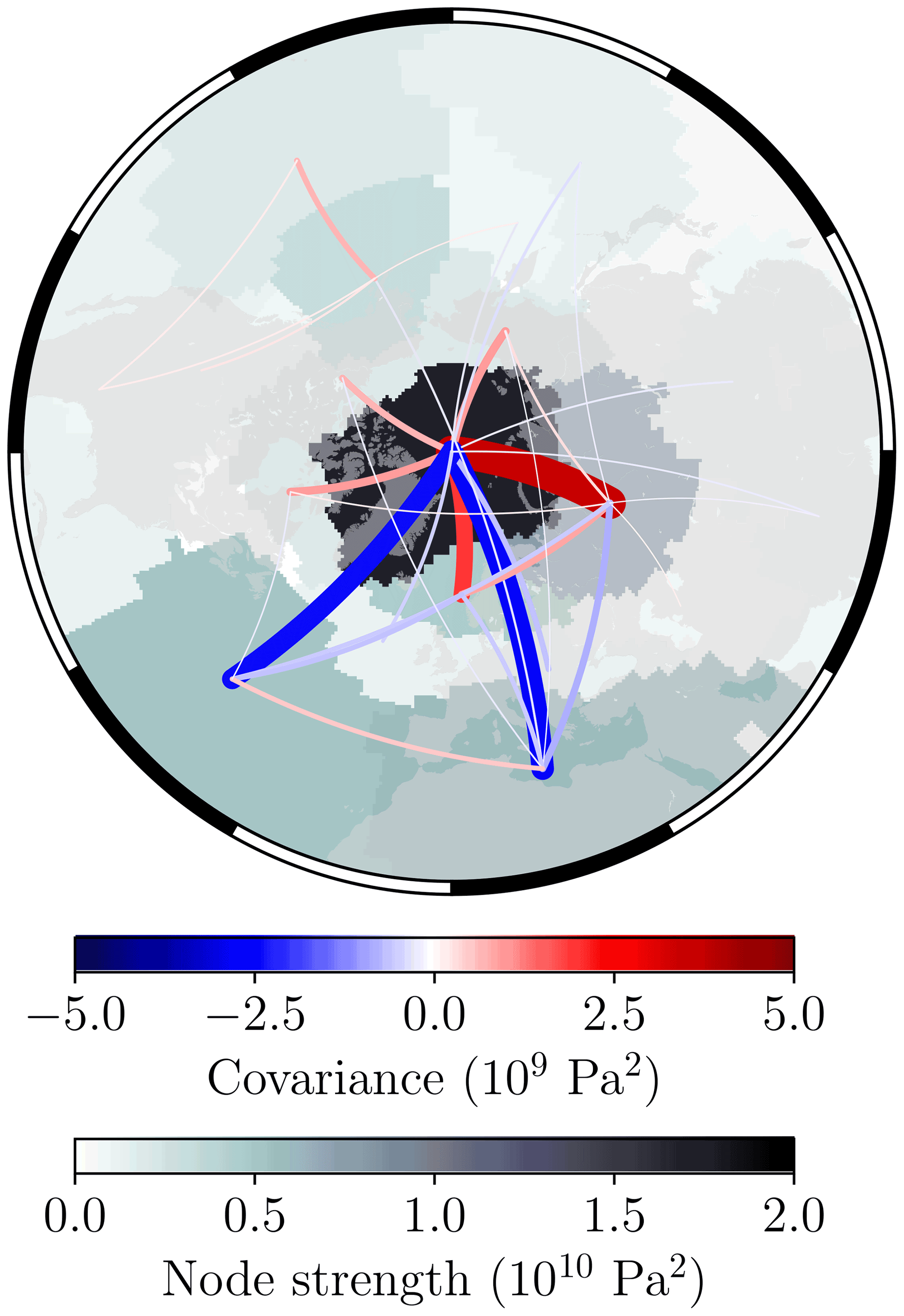
Figure 1Complex network of DJFM mean sea-level pressure from ERA5, computed between 1979 and 2020. The covariance-based link weights are computed from Eq. (2), in which the thickness of each link is proportional to the covariance. Only links which have a corresponding p value <0.10 are shown here to aid visualisation. The strength of each node is then computed from Eq. (3).
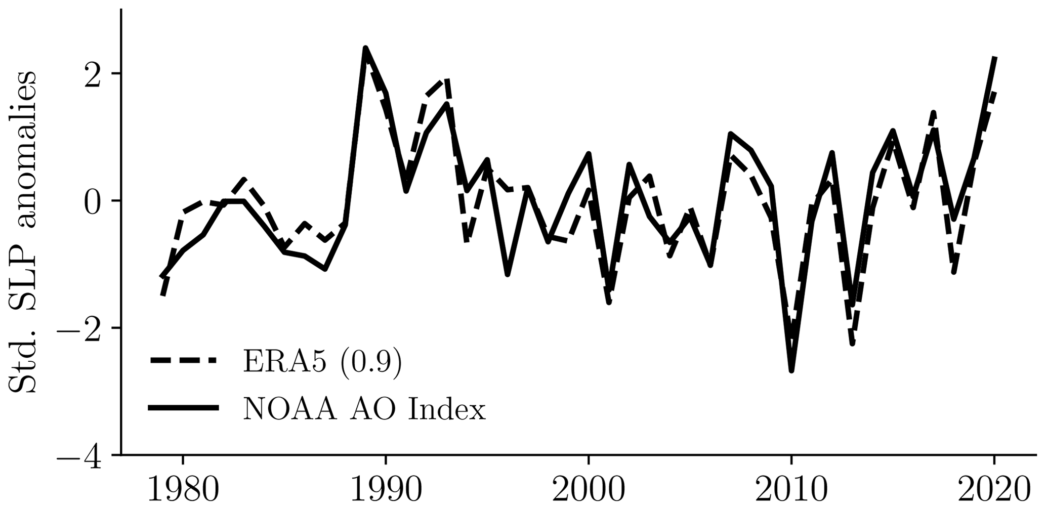
Figure 2The standardised (Std.) temporal component of DJFM mean sea-level pressure (SLP) variability from ERA5 (dashed curve). Temporal components are computed via Eq. (1), in which this time series is extracted from the ERA5 network node with the highest strength. The number in parentheses corresponds to the correlation coefficient with the DJFM AO index from the National Oceanic and Atmospheric Administration (NOAA; available from https://www.cpc.ncep.noaa.gov/products/precip/CWlink/daily_ao_index/ao.shtml, last access: 1 June 2021).
In general, we can consider a network as a group of vertices, or nodes, whereby each node k may be connected to any other node in the network l via a weighted edge, or link. Subsequently, in our implementation a climate network of N nodes corresponds to time series data, , representing n regularly sampled observations in time, , at N fixed geographical locations, and the links represent statistical interdependencies between any pair of node time series gk and gl. In more detail, let us define as a zero-mean (the linear trend is removed from each grid cell) time series data set (e.g. DJFM mean sea-level pressure anomalies or JJAS sea ice concentration anomalies), which represents n regularly sampled observations in time at P fixed geographical locations such that . The N network nodes are then derived by implementing a grid-based clustering algorithm to the input data set so that the dimensionality of X is reduced from P to N (see Gregory et al., 2020 for further details of this clustering step). Each cluster (node) then corresponds to a particular pattern of climate variability and represents a spatial region of, for example, summer sea ice concentration or winter sea-level pressure that has behaved in a homogeneous way over the length of the time series record. We can then generate links between the nodes by first computing the cumulative anomaly time series of each network node, which for a given node 𝒞k is taken as the sum of the grid-cell-weighted de-trended time series of all cells within that node:
where wp=cos (θp) for a regular latitude–longitude grid (sea-level pressure data), where θp is the latitude of grid cell p, or simply wp=dp for a polar stereographic area grid (sea ice concentration data), where dp is the area in square kilometres of grid cell p. Subsequently, the link weight between two nodes k and l is calculated as the temporal covariance between two network node anomaly time series:
where 𝔼[⋅] is the expected (mean) value. Finally, we define the weighted degree, or strength, of a given network node 𝒮k as the sum of the absolute value of all its associated link weights:
The nodes with the highest strength are commonly referred to as the hubs of the network (Tsonis and Roebber, 2004), and they represent the dominant patterns of variability in the input data set X. By this definition, the node with the highest strength belonging to the network of mean sea-level pressure data can be considered a good proxy for the AO. Note also that this network framework allows for weighted links between nodes of a single network (as detailed above) and also between nodes of multiple networks (i.e. between nodes of sea-level pressure and sea ice concentration), which is used to assess the winter AO to summer sea ice teleconnection in Sect. 4.3.
Figure 1 shows the network structure of DJFM mean sea-level pressure data from ERA5. In this case we can see how the network nodes correspond to a set of spatially contiguous areas, where for a given node, each grid cell is weighted by the strength of the node in which that cell belongs. The node with the highest strength in Fig. 1 can be considered as a proxy for the spatial pattern of variability in the AO, and from this map we can see that this corresponds to the large node situated over the majority of the Arctic Ocean, Greenland, the Canadian Archipelago, and parts of northern Russia. The weighted links then illustrate how each of the nodes have covaried relative to each other over the period 1979–2020, and indeed we notice the out-of-phase relationship (negative covariance) between the AO node and the mid-latitude Atlantic sector, highlighting the dipole nature of the North Atlantic Oscillation (Hurrell et al., 2003). We can also extract the temporal component of variability from the “AO node” (Fig. 2), which produces a very consistent signal with the standard AO index as defined by the National Oceanic and Atmospheric Administration (NOAA), highlighting the robustness of the complex networks method. It is worth noting however that in Fig. 2, and indeed for the rest of this paper, we reverse the sign of the temporal component of each node of the winter sea-level pressure networks (from ERA5 and CMIP6 data) in order to be consistent with the standard AO index, for which positive AO index values correspond to low atmospheric pressure, and similarly negative AO index values correspond to high atmospheric pressure.
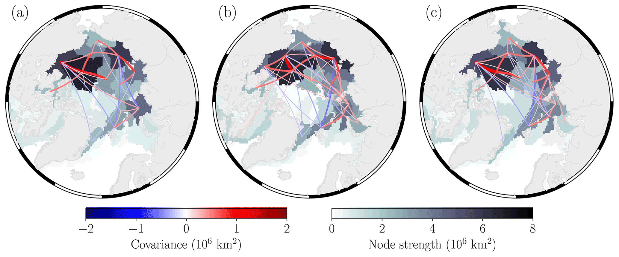
Figure 3Complex networks of JJAS sea ice concentration for (a) NASA Team, (b) Bootstrap, and (c) OSI-SAF data sets, computed between 1979 and 2020. Only links which have a p value <0.10 are shown here to aid visualisation.
In Fig. 3 we show similar networks for JJAS sea ice concentration from each of the observational products. Here we can see how the dominant patterns of summer sea ice variability (i.e. highest node strengths) are typically in the East Siberian and Laptev seas, as well as the Canada Basin. Each observational product generally shows the same structure of largely positive covariance between network nodes and the out-of-phase connection between the Fram Strait and the Pacific sector. The magnitude of the node strengths between the observational data sets somewhat varies in the dominant regions of variability, with the Bootstrap product showing the largest strengths in the East Siberian and Laptev seas. In the next section we introduce two global metrics for deriving quantitative measures of similarity between networks.
3.2 Metrics for comparing networks
Before we introduce the two metrics which are used to compare similarities between complex networks, it is worth saying a few words about what information we can expect to obtain when comparing models and observations/reanalysis. Due to the fact that any CMIP6 model ensemble member is in its own phase of internal variability (e.g. Hawkins and Sutton, 2009; Notz, 2015), we cannot expect to find consistency in the sign and magnitude of anomalies between, for example, the ERA5 AO time series and that of any one model ensemble member (and similarly for sea ice); therefore it would not be prudent to perform any analysis which makes direct comparisons of any time series between observational and CMIP6 network nodes. We can however expect a model with accurate physics to reproduce similar dominant regions of variability as the observations and the same sign and magnitude of the inter-connected links between nodes, e.g. the strong negative coupling between the AO and sea-level pressure anomalies in the North Atlantic and the weak negative coupling with the North Pacific (see Fig. 1), and similarly we can expect the same regional responses of Arctic sea ice to different phases of the AO between observations and models. The two metrics we introduce in the coming sections provide a way to quantify similarities in the locations which the observations and models define as the dominant regions of variability, as well as the connectivity of these regions, without explicitly comparing network node time series.
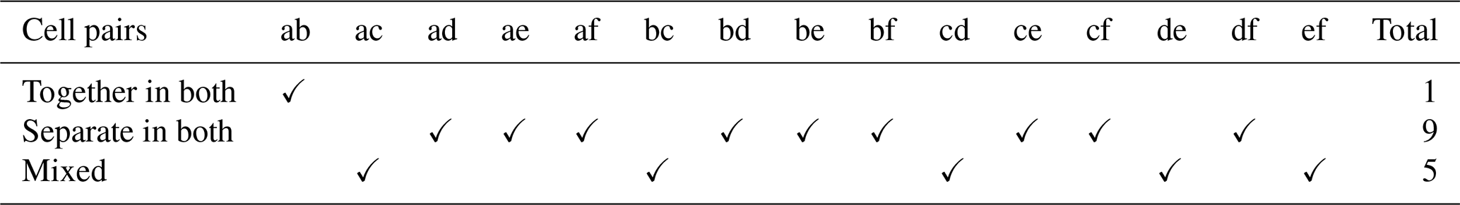
Table 2Synthetic example of cell clusters to illustrate the concept of the Rand index (see Sect. 3.2.1), based on Rand (1971).
3.2.1 Adjusted Rand index
The adjusted Rand index (ARI; Hubert and Arabie, 1985) is a metric which is often used to evaluate similarities between sets of clusters (Steinley, 2004), and as such we use it here to compare how two networks have clustered grid cells together to form their spatially contiguous set of network nodes and subsequently their spatial patterns of either sea-level pressure or sea ice concentration variability. To understand the ARI, it is worth briefly introducing the (un-adjusted) Rand index by following the example outlined by Rand (1971). First, consider two different synthetic networks which have clustered grid cells together in two distinct ways.
In these two simple network constructions, there are three nodes in each network, in which each node contains a clustering of cells labelled a–f. The Rand index then measures similarities and differences in the clustering of these cells by analysing all the possible cell pairings between the two networks (see Table 2). In this example there are a total of 10 similarities (grid cells which are clustered together in both networks and grid cells which are separate in both networks) out of a possible 15 pairings, which gives a Rand index score of . The ARI is then an update of the Rand index which takes into account the fact that grid cells could be clustered together by chance (see Hubert and Arabie, 1985, for further details). In the synthetic example above, the ARI corresponds to 0.07 – note that the ARI varies between 0 (totally dissimilar clustering) and 1 (identical clustering). Computing the ARI between, for example, the NASA Team and OSI-SAF summer sea ice concentration networks produces a value of 0.69, showing relatively consistent clustering (as we saw qualitatively in Fig. 3).
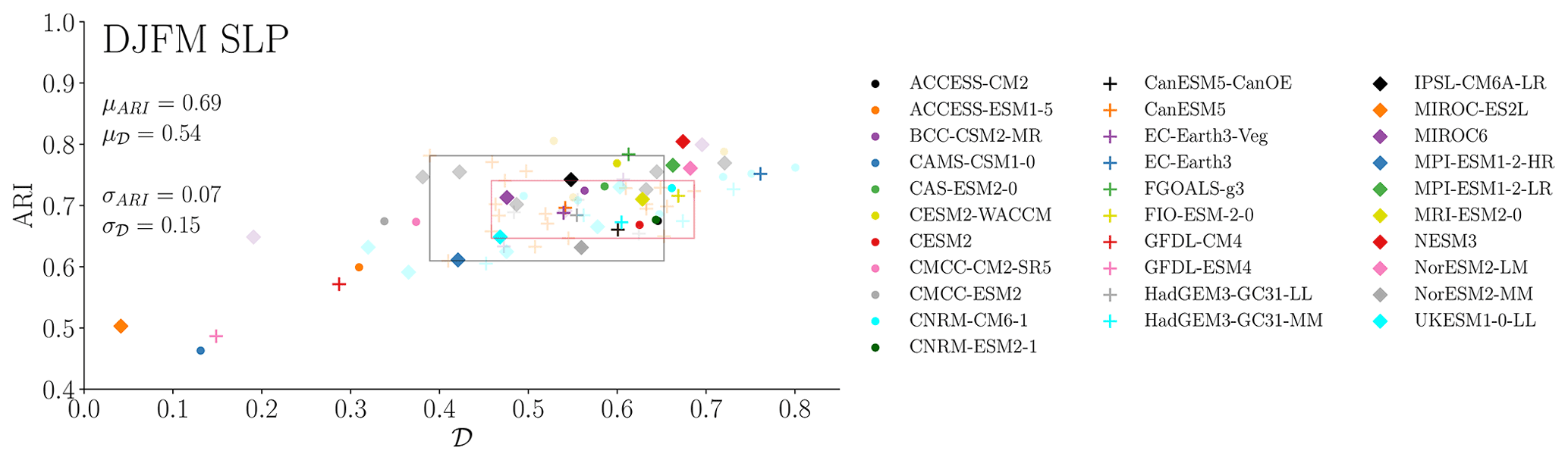
Figure 4ARI and 𝒟 metrics for winter sea-level pressure (SLP) networks computed between 1979 and 2020 for every ensemble member for 31 different CMIP6 models (74 realisations), relative to ERA5 atmospheric reanalysis. The semi-transparent colours represent individual ensemble members (for which the number of ensemble members is greater than 1), and the opaque colours are the mean of all ensemble members. The mean and standard deviation across all points are given by μ and σ, respectively. The grey and red boxes represent the range of ARI and 𝒟 values for 10 CanESM5 ensemble members each, in which members in each box have the same physics and forcing but slightly perturbed initial conditions, while the two boxes separate groups based on model physics (i1p1f1 and i1p2f1). See Sect. 4.1.
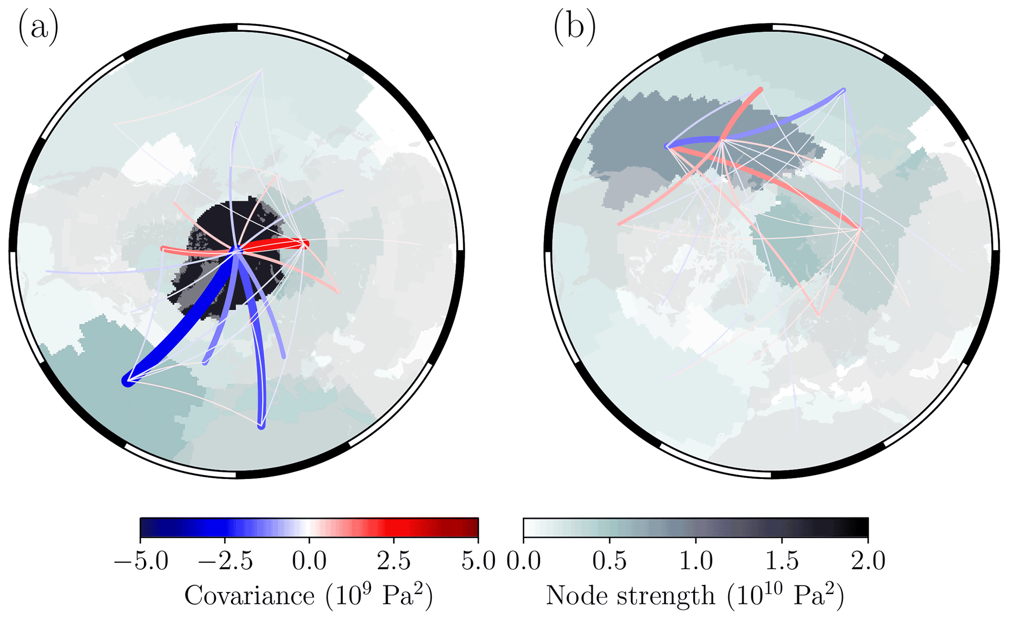
Figure 5Winter sea-level pressure networks from (a) CNRM-CM6-1 (ensemble member: r6i1p1f2) and (b) MIROC-ES2L (ensemble member: r1i1p1f2), computed between 1979 and 2020. The CNRM-CM6-1 model produces ARI and 𝒟 values of 0.76 and 0.80, respectively, while the MIROC-ES2L model produces values of 0.50 and 0.04, respectively. Only links which have a corresponding p value <0.10 are shown here to aid visualisation.
3.2.2 Network distance metric
The network distance metric (𝒟; Fountalis et al., 2015) provides a way to compare networks in terms of both the spatial extent of their network nodes and also their node strengths. Recall that node strength incorporates information about the connectivity of a particular node (i.e. the magnitude of all its connected links); hence when comparing the strength of a particular region between models and observations, we can infer which one has a larger degree of covariability across the network. This allows us to deduce whether the models over- or underestimate the magnitude of variability in a particular region without comparing node time series. Consider, for example, the underlying map of node strengths in Fig. 3. We can compute 𝒟 by first taking the sum of the absolute difference between two of these “strength maps”, M1 and M2 (e.g. NASA Team and OSI-SAF), and then normalising by the sum of the absolute difference between random permutations of both network strength maps, and :
A value of 𝒟=1 means that both networks are identical in their node strengths and spatial extent of nodes, whereas a value close to 𝒟=0 implies that the two networks are as similar as a random assignment of node strengths to grid cells. Computing 𝒟 between the NASA Team and OSI-SAF summer sea ice concentration networks produces a value of 0.86. The combination of ARI and 𝒟 allows us to infer various properties between two networks. For example, when ARI =1 and 𝒟=0, this suggests that two networks agree in terms of which grid cells have behaved homogeneously over the length of the time series record in order to cluster together to form network nodes; however they disagree in terms of the magnitude of variability in the nodes. On the other hand, if ARI is close to 0 and 𝒟 is close to 1, then this implies that the magnitude of variability across the networks is relatively consistent; however the geographic areas which are clustered together to form network nodes are considerably different. Two networks can then be considered identical if ARI and 𝒟=1.
4.1 Sea-level pressure networks in CMIP6
For every available ensemble member from each of the CMIP6 models outlined in Table 1, we compute individual complex networks of DJFM sea-level pressure over the period 1979–2020 and then compute ARI and 𝒟 metrics relative to the ERA5 sea-level pressure network. In Fig. 4 we can see how the spread in 𝒟 values across all model ensemble members is over twice as large as for the ARI values, which suggests large disagreement between ensemble members on the degree of connectivity of network nodes and hence the magnitude of regional sea-level pressure variability. Note that the apparent linear relationship between ARI and 𝒟 is to be expected given that both metrics encapsulate information related to the spatial agreement of network nodes between models and ERA5. Across all models, CNRM-CM6-1 (ensemble member r6i1p1f2) produces the most similar network structure to ERA5, with ARI =0.76 and 𝒟=0.80. Figure 5 shows the corresponding network for CNRM-CM6-1 r6i1p1f2 and also MIROC-ES2L r1i1p1f2. The MIROC-ES2L r1i1p1f2 ensemble member produces the most dissimilar network structure relative to ERA5, with ARI and 𝒟 of 0.50 and 0.04, respectively. The networks show how CNRM-CM6-1 produces the relatively consistent node of high strength over the Arctic Ocean (similar to ERA5 in Fig. 1) and also shows the same strong negative linkage with the mid-latitude Atlantic sector and weak linkage with the Pacific sector. On the other hand, MIROC-ES2L shows significantly different regions of variability than ERA5, and also weaker connectivity, with overall weaker link weights and very low strength over the Arctic Ocean. At this point it is worth noting that for models with several ensemble members which all contain the same physics and forcing but slightly perturbed initial conditions, we can inspect the spread in ARI and 𝒟 values across these particular ensemble members to gain an insight into the contributions of internal variability to the resultant network structures (relative to ERA5). The CanESM5 model is the only model here with enough ensemble members to approximate a “large ensemble” (e.g. Kay et al., 2015) with 20 members; however these in turn comprise two groups of 10 members with different physics (shown by the grey and red boxes in Fig. 4). While each box is likely to be under-representative of the true spread due to internal variability with only 10 members, it does provide some initial insight. Interestingly the spread in 𝒟 values between the two boxes is relatively consistent, although the spread in ARI differs by a larger amount depending on model physics. In this example, the difference in model physics also appears to shift the mean value of 𝒟, which may illustrate how model physics ultimately plays a role in how the spatio-temporal patterns of variability are represented. To see the influence of internal variability on the network structure first hand, Supplement Fig. S1 shows winter sea-level pressure networks for the CanESM5 ensemble members within the red box in Fig. 4, where it can be seen that despite some differences in relative node strengths, each ensemble member produces a network with the strongest node centred over the Arctic Ocean, as well as high node strengths over the Pacific. These two large node areas across the ensemble members are likely what drives the low spread in ARI values, while the large spread in 𝒟 values is due to the relative discrepancies in node strengths of these regions. This suggests that internal variability plays a larger role in governing the magnitude of regional sea-level pressure variability than in governing the actual spatial patterns themselves.
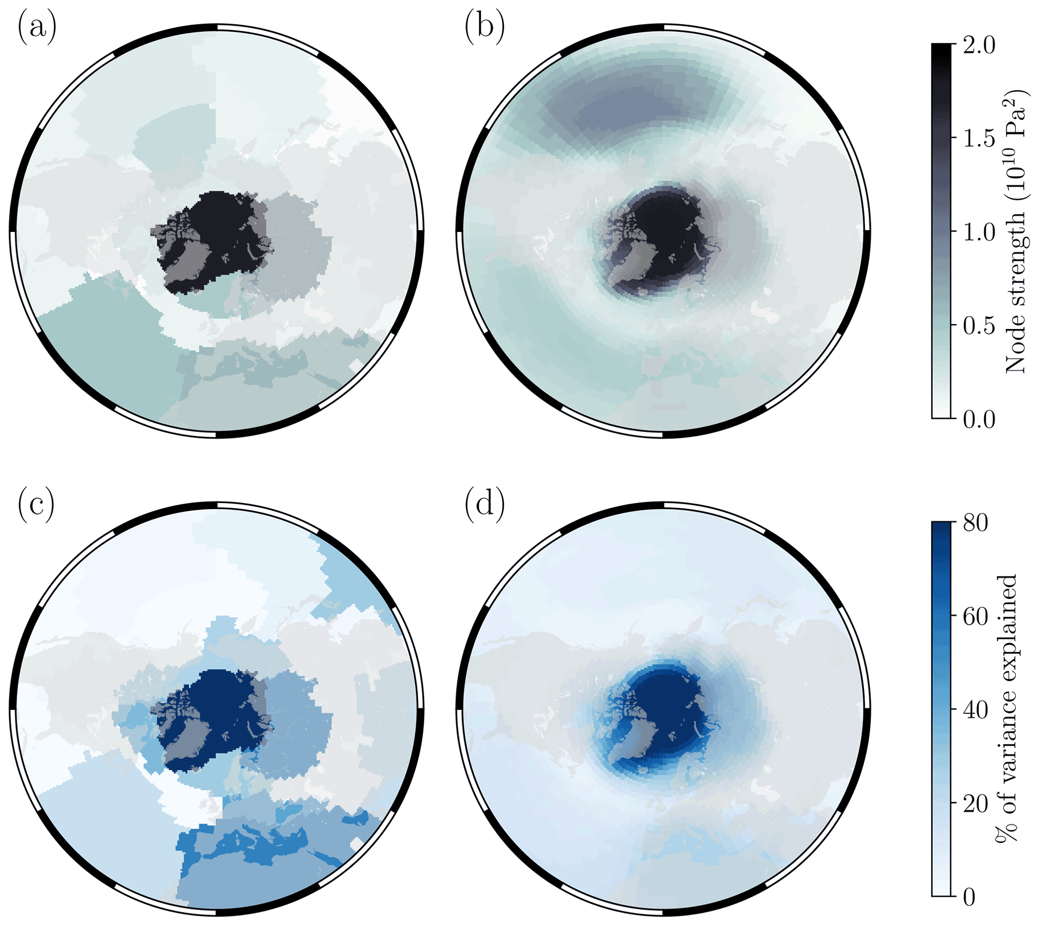
Figure 6(a–b) The spatial patterns of winter sea-level pressure variability (node strengths) from (a) ERA5 and (b) the average of all 74 CMIP6 model ensemble members. (c–d) The percentage of variance in mean Northern Hemisphere winter sea-level pressure explained (e.g. Donges et al., 2015) by network nodes in (c) ERA5 and (d) the average of all 74 CMIP6 model ensemble members.
In Fig. 6a–b we now average each of the network strength maps across all of the CMIP6 model ensemble members and compare this with the ERA5 strength map. While this removes the ability to identify individual network nodes and their links, it does allow us to qualitatively assess how CMIP6 models, on average, represent the spatial patterns of winter sea-level pressure variability and their degree of connectivity. We notice, for example, that on average CMIP6 models represent the spatial pattern of the AO relatively well, although they slightly underestimate its node strength. Furthermore, node strengths in the north-western Pacific Ocean appear to be overestimated on average, while they are underestimated over northern Africa and southern Europe. In Fig. 6c–d we also show the percentage of variance in mean Northern Hemisphere sea-level pressure anomalies that is explained by each ERA5 network node, as well as the average of CMIP6 nodes (the mean sea-level pressure anomalies in CMIP6 models are computed for each individual model ensemble member, and then the percentage of variance is computed between this signal and its own respective sea-level pressure network nodes). We can see that the nodes centred over the Arctic Ocean explain the highest percentage of variance in Northern Hemisphere sea-level pressure in both ERA5 and CMIP6 networks; however the models underestimate the relative importance of the North Atlantic and northern Africa–southern Europe region in explaining winter sea-level pressure variability. It is also worth mentioning that although the CMIP6 models identify the North Pacific as a region of strong covariability (Fig. 6b), the percentage of variance explained by this region is relatively low. This can occur due to the fact that network nodes which are larger in spatial extent will naturally show higher covariance with other regions (and hence node strengths) because the temporal component of variability of a given node corresponds to the sum of all grid cell time series within that node (see Eq. 1). If however a node's correlation (i.e. standardised covariance) with the mean sea-level pressure signal is relatively small, then this results in a squared reduction in percentage of variance explained (recall that fraction of variance explained equals correlation squared). This therefore suggests that sea-level pressure over the North Pacific Ocean in CMIP6 models is more spatially homogeneous than ERA5 (recall that an individual network node represents a geographic region which has behaved in a similar way over the length of the time series record).
4.2 Sea ice concentration networks in CMIP6
In this section we compute individual complex networks of JJAS sea ice concentration over the period 1979–2020 for every available ensemble member from each of the CMIP6 models and then compute ARI and 𝒟 metrics relative to the NASA Team, Bootstrap, and OSI-SAF sea ice concentration networks. In Fig. 7 we see a lower spread in ARI values compared to the 𝒟 values, which, similar to the sea-level pressure networks, suggests that CMIP6 ensemble members show large disagreement on the degree of connectivity of network nodes and hence the magnitude of regional sea ice concentration variability. What is perhaps noticeable is that the models which appear to perform better in terms of their summer sea ice ARI and 𝒟 scores are not necessarily the same as those that score well for their winter sea-level pressure networks – discussed further in Sect. 5. In Fig. 8 we show sea ice concentration networks from the MIROC6 (r1i1p1f1) and the CAMS-CSM1-0 (r1i1p1f1) models. The MIROC6 model produces closer patterns of variability to the observations than other CMIP6 models, with ARI values of 0.48 (NASA Team), 0.48 (Bootstrap), and 0.47 (OSI-SAF) and 𝒟 values of 0.66 (relative to each observational network). Having said that, we can see that the spatial extent and strength of the node in the Beaufort Sea–Canada Basin are somewhat underestimated (relative to the observational networks shown in Fig. 3) and that the node strength in the Laptev Sea is overestimated, and interestingly its link between the Beaufort Sea and the East Siberian Sea is negative. It does however produce consistent out-of-phase network links between the Fram Strait and the Eurasian–Pacific sectors of the Arctic. The CAMS-CSM1-0 model produces a more dissimilar score with ARI values of 0.33 (NASA Team), 0.30 (Bootstrap), and 0.33 (OSI-SAF) and 𝒟 values of 0.28 (NASA Team), 0.30 (Bootstrap), and 0.29 (OSI-SAF). The low 𝒟 values are being caused by the significant overestimation in the link weights, and hence node strengths, in the Greenland, Iceland, and Norwegian seas, Barents Sea, East Siberian Sea, and Laptev Sea (notice how the link weights and node strengths in this model are in some cases an order of magnitude higher than the observational networks). Once again, we can highlight the spread in ARI and 𝒟 for ensemble members within the two unique model physics groups of the CanESM5 model to gain an insight into the contributions of internal variability to the resultant network structures (relative to the satellite-derived observations). Similar to the sea-level pressure example, here the spread in 𝒟 for the CanESM5 model is larger than the spread in ARI, and a difference in model physics acts to shift the mean value of 𝒟. Supplement Fig. S2 then shows the summer sea ice concentration networks for the CanESM5 ensemble members within the red boxes in Fig. 7. While the majority of members show the strongest nodes within the eastern sector of the Arctic, the relative differences in node strengths are somewhat large. Analogous to the discussion in Sect. 4.1, this may highlight how internal variability plays a larger role in governing the magnitude of regional sea ice concentration variability than in governing the spatial patterns themselves.
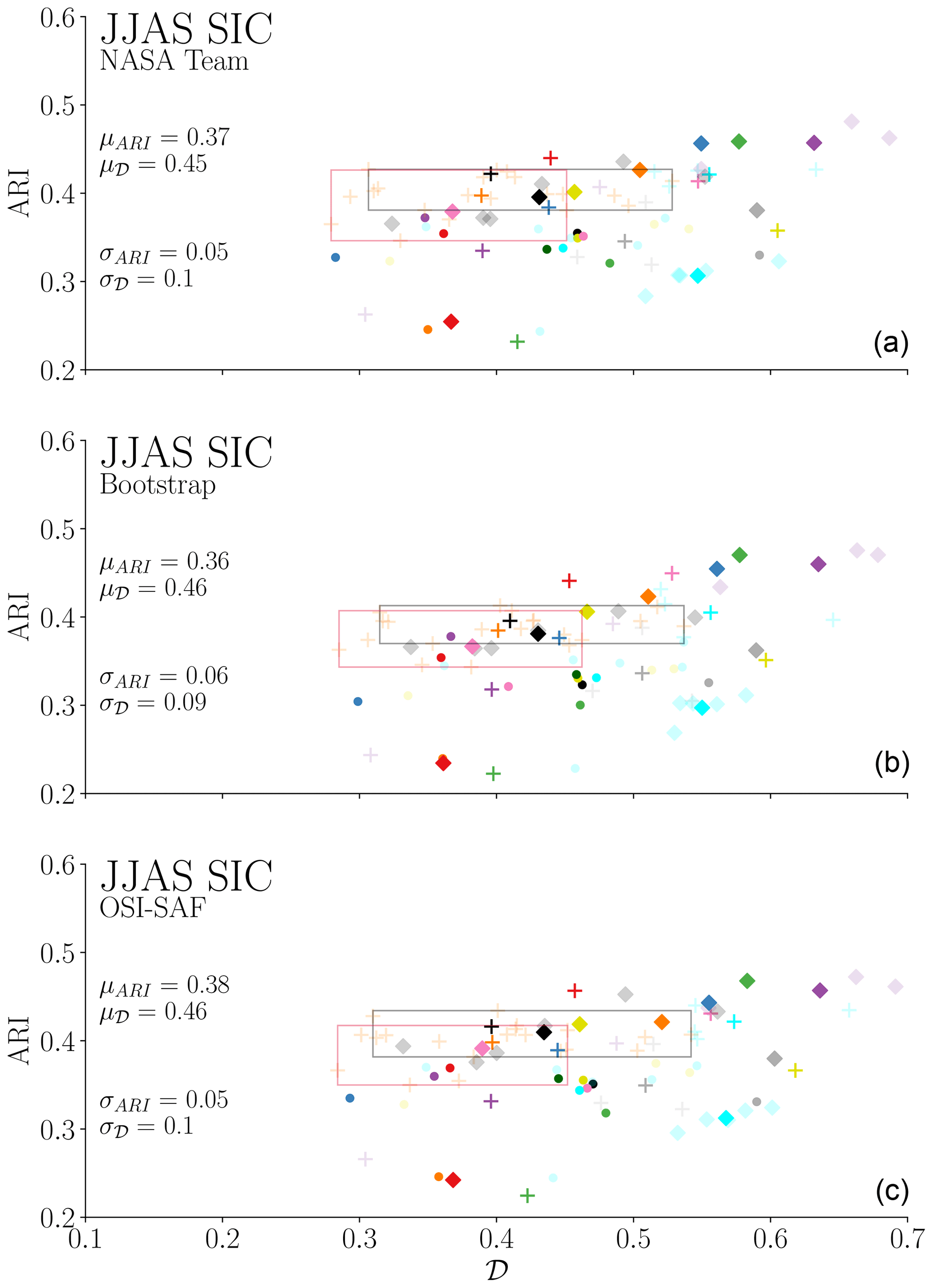
Figure 7ARI and 𝒟 metrics for summer sea ice concentration (SIC) networks computed between 1979 and 2020 for every ensemble member for 31 different CMIP6 models (74 realisations). ARI and 𝒟 are computed relative to NASA Team (a), Bootstrap (b), and OSI-SAF (c) observational networks. The symbols and colours of each point, as well as the red and grey boxes, are consistent with Fig. 4.
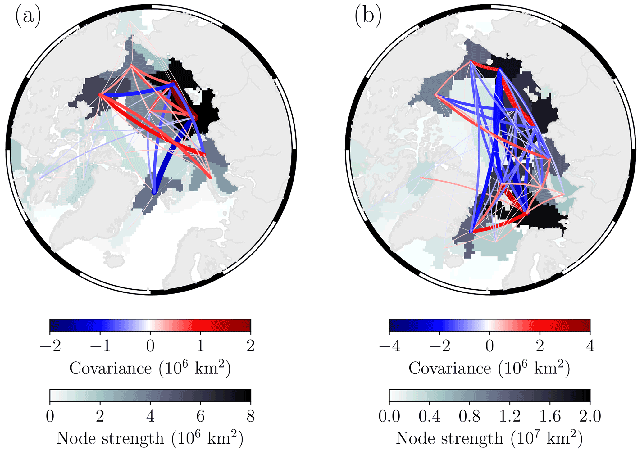
Figure 8Summer sea ice concentration networks from (a) MIROC6 (ensemble member: r1i1p1f1) and (b) CAMS-CSM1-0 (ensemble member: r1i1p1f1), computed between 1979 and 2020. The MIROC6 model produces average ARI and 𝒟 values of 0.48 and 0.66, respectively (average of metrics computed relative to NASA Team, Bootstrap, and OSI-SAF networks), while the CAMS-CSM1-0 model produces average values of 0.32 and 0.29, respectively. Only links which have a corresponding p value <0.10 are shown here to aid visualisation.
In Fig. 9a–b we average each of the network strength maps across both the observational data and all of the CMIP6 model ensemble members. Here we notice that, on average, the models show the dominant regions of variability are in the East Siberian and Laptev seas, although the node strengths are somewhat overestimated relative to the observations. Furthermore, while the observations outline the Beaufort Sea–Canada Basin as the region of highest connectivity (more so than the East Siberian–Laptev seas), the models show relatively little connectivity here on average. In Fig. 9c–d we also show the percentage of variance in pan-Arctic summer sea ice area that is explained by each observational network (averaged) and the average of CMIP6 model ensemble members. In this case the models generally underestimate the importance of regions such as the Beaufort, East Siberian, and Laptev seas in explaining the variance in pan-Arctic summer sea ice area and overestimate the percentage of variance explained in regions such as the Barents Sea and parts of the Eurasian Basin. Once again, we also see how the regions of highest strength are not necessarily the ones which explain the highest percentage of variance in pan-Arctic sea ice area in the models, which suggests that the models may be overestimating the spatial extent of the network nodes in the Eurasian seas, causing them to covary more strongly with other nodes despite having perhaps lower absolute correlation with the pan-Arctic sea ice area signal.
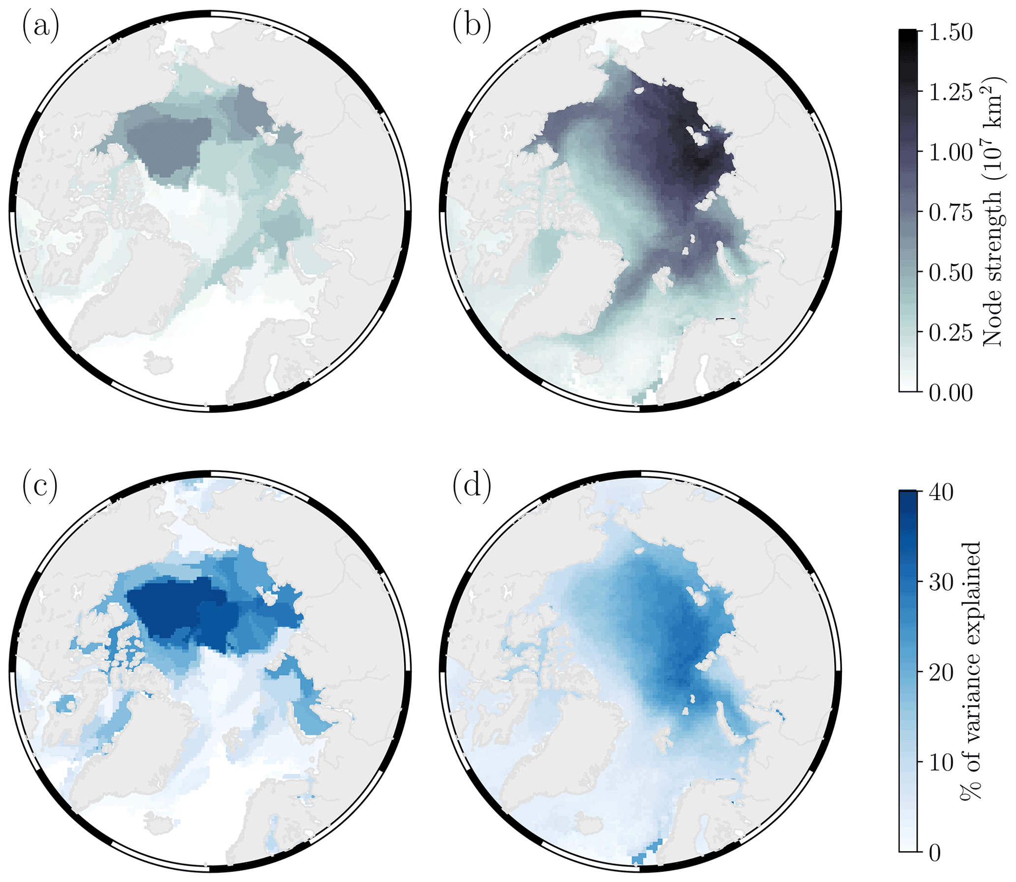
Figure 9(a–b) The average spatial patterns of summer sea ice concentration variability (node strengths) from (a) the three observational data sets and (b) all 74 CMIP6 model ensemble members. (c–d) The percentage of variance in pan-Arctic summer sea ice area explained by network nodes in (c) the three observational data sets and (d) the average of all 74 CMIP6 model ensemble members.
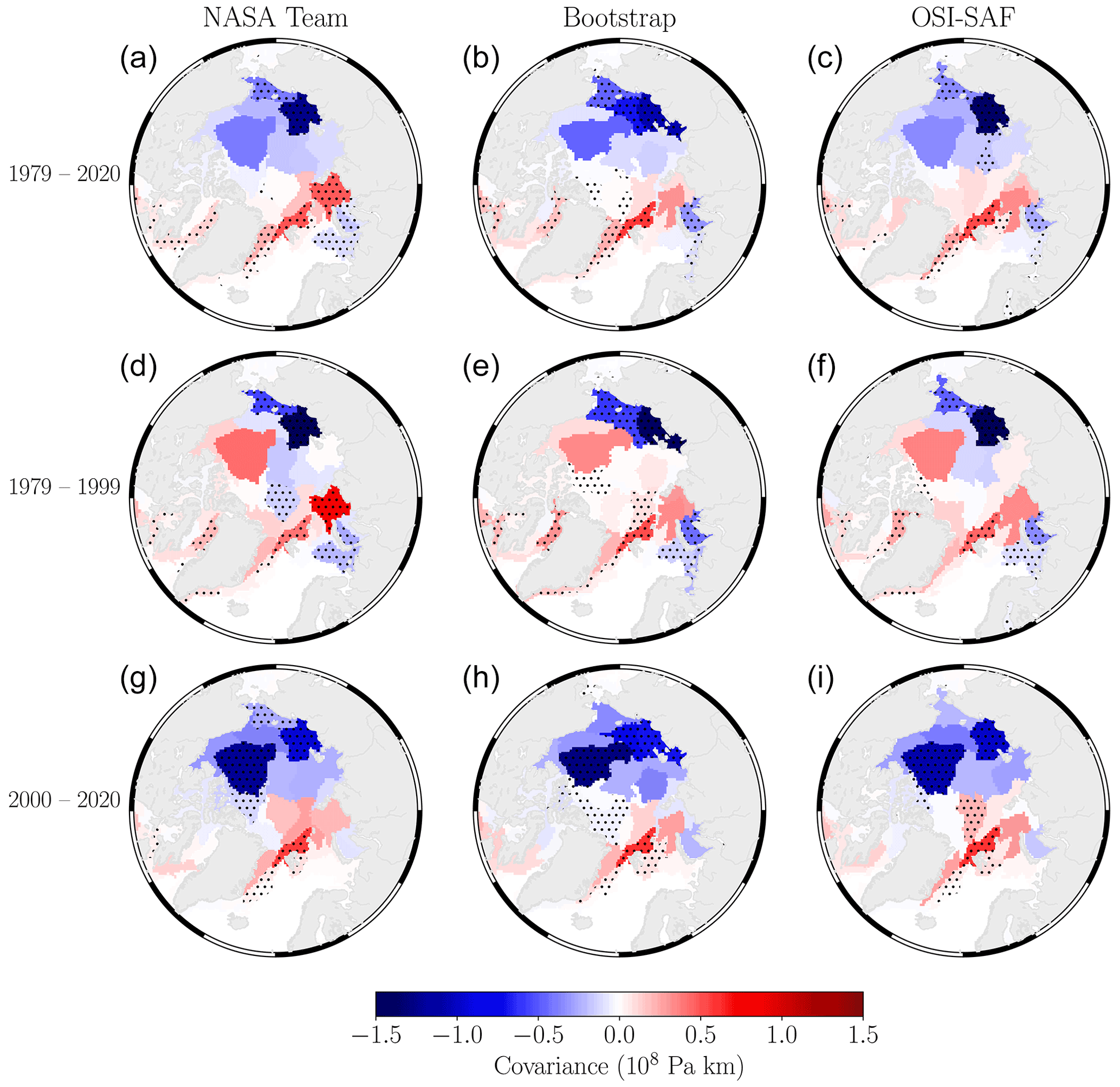
Figure 10Network link weight between the DJFM ERA5 “AO node” (dashed time series from Fig. 2) and each of the JJAS sea ice concentration network nodes, computed between (a–c) 1979 and 2020, (d–f) 1979 and 1999, and (g–i) 2000 and 2020. The columns from (a) to (i) show the corresponding maps for NASA Team, Bootstrap, and OSI-SAF data sets. Stippling denotes links with p values <0.05.
4.3 AO to sea ice teleconnection
We now turn to an investigation of the winter AO to summer sea ice teleconnection. We begin by illustrating how we can use the network framework to exploit this relationship in the observational and reanalysis data by effectively considering both winter sea-level pressure and summer sea ice concentration networks as individual layers within a multi-layer network (Boccaletti et al., 2014). We also briefly investigate whether this teleconnection may be changing over time, before ultimately performing the same analysis for each of the CMIP6 models. A discussion of the results in this section is then presented in Sect. 5.
4.3.1 Observations/reanalysis
In this section we use the temporal component of variability associated with the “AO node” of the ERA5 sea-level pressure network to define the time series corresponding to the winter AO (i.e. the dashed time series in Fig. 2). We then generate links between the winter AO and summer sea ice as the temporal covariance (Eq. 2) between this AO time series and each of the nodes of the summer sea ice concentration networks from each of the observational data sets. In Fig. 10 we use the same concept as the strength maps shown previously but instead weight each grid cell by the link weight (temporal covariance) between the AO and sea ice concentration node time series. In the first row of Fig. 10 we compute the link weights using the entire observational period (1979–2020), in which we notice a very strong anti-correlation between the winter AO and summer sea ice in the East Siberian Sea across all observational products (standardising the link weight for this node produces correlation coefficients of −0.65, −0.57, and −0.66 for the NASA Team, Bootstrap, and OSI-SAF data sets, respectively). Furthermore, all of the summer sea ice nodes in the Eurasian–Pacific sector of the Arctic exhibit varying degrees of anti-correlation with the winter AO, while the Atlantic sector shows largely positive covariance and is particularly strong in the Fram Strait region. If we then analyse the covariance between the first half (1979–1999) and second half (2000–2020) of the observational record (second row and third row of Fig. 10, respectively), we notice some interesting patterns. In particular, the correlation across the whole Eurasian–Pacific sector of the Arctic has been more strongly negative since 2000, especially within the Canada Basin. The reverse of sign in the Canada Basin may not be significant given the moderate degree of positive correlation between 1979 and 1999; however the strong negative correlation between 2000 and 2020 implies that positive AO winters (anomalously low sea-level pressure) now typically lead to anomalously low summer sea ice concentration anomalies across both the eastern and western Arctic, whereas previously this typically only occurred in the eastern Arctic (see also Mallett et al., 2021, for a recent investigation of this changing relationship). It is also worth noting that summer sea ice in the Atlantic sector has generally remained positively correlated with the winter AO over both halves of the observational period – see Sect. 5 for further discussion.
4.3.2 CMIP6 models
For each CMIP6 model ensemble member we extract the temporal component from the node with the highest strength of each winter sea-level pressure network and compute the covariance-based link weight with each node of its respective summer sea ice concentration network. In Fig. 11, we show an adaptation of the network comparison metrics shown in Fig. 7. In this case, rather than computing the distance metric 𝒟 as the normalised sum of the difference between observational and CMIP6 model strength maps, we instead create the corresponding “link maps” for each model ensemble member (i.e. the equivalent of the maps shown in Fig. 10) and compute 𝒟 relative to the observational link maps. The ARI metric is computed as before; hence ARI values presented in Figs. 7 and 11 are identical. The values reported in Fig. 11 are for link weights computed over the entire period (1979–2020), and with average distance values of 0.26, 0.27, and 0.26 relative to NASA Team, Bootstrap, and OSI-SAF, respectively, we can see that the models perform quite poorly at replicating the observed network links between the winter AO and summer sea ice – recall that for 𝒟=0, the two maps are as dissimilar as a random assignment of link weights to grid cells. The equivalent plots for the periods 1979–1999 and 2000–2020 are shown in Supplement Figs. S4 and S5, respectively. Figure 12 shows two examples of CMIP6 ensemble member link maps for the winter AO to summer sea ice teleconnection between 1979 and 2020. The MIROC6 model (r1i1p1f1) was shown in Fig. 8 to be a network which produced relatively similar patterns of summer sea ice variability compared to the observations, and here it is one of the models with the highest similarity score in terms of its AO to sea ice teleconnection, with 𝒟 values of 0.43 (NASA Team), 0.43 (Bootstrap), and 0.41 (OSI-SAF). We can see that it also captures the strong negative covariance linkage with the East Siberian Sea; however it overestimates the connection within the Laptev Sea and does not capture the negative link with the Beaufort Sea or strong positive link with the Fram Strait. The EC-Earth3-Veg model (r4i1p1f1) produces the lowest 𝒟 scores at 0.06 (NASA Team), 0.07 (Bootstrap), and 0.06 (OSI-SAF). This is both due to the difference in sign of many of the AO to sea ice node link weights compared to the observations (e.g. Kara and Beaufort seas) and also due to its inability to represent the similar regions of sea ice variability as the observations. Returning to the subject of internal variability, Supplement Fig. S3 shows the corresponding AO to sea ice teleconnections for each ensemble member of the CanESM5 model within the red boxes of Fig. 11, computed between 1979 and 2020. This figure highlights that, across all the ensemble members, the general patterns show negative covariance in the eastern Pacific sector of the Arctic and positive covariance in the western Pacific and Atlantic sectors, somewhat in agreement with the observations. Comparing ensemble members highlights how the magnitude of these connections can vary considerably, as discussed in Sect. 4.1 and 4.2.
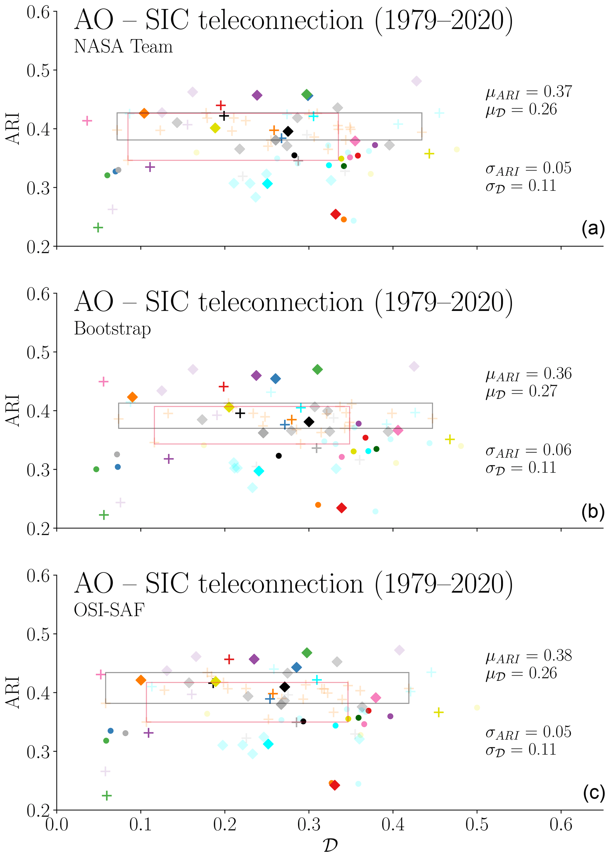
Figure 11ARI and 𝒟 metrics for comparing observation and CMIP6 model summer sea ice concentration networks and the winter AO to summer sea ice teleconnection for every ensemble member for 31 different CMIP6 models (74 realisations). ARI and 𝒟 are computed relative to NASA Team (a), Bootstrap (b), and OSI-SAF (c) observational networks. Network distance values (𝒟) are computed from observation and model “link maps” as shown in Fig. 10. The symbols and colours of each point, as well as the red and grey boxes, are consistent with Fig. 4.

Figure 12Covariance-based link weights between the winter AO node time series and each node of the summer sea ice concentration network between 1979 and 2020 for (a) MIROC6 (ensemble member: r1i1p1f1) and (b) EC-Earth3-Veg (ensemble member: r4i1p1f1). The MIROC6 model produces average ARI and 𝒟 values of 0.48 and 0.42, respectively, while the EC-Earth3-Veg model produces values of 0.26 and 0.06, respectively. Stippling denotes links with p values <0.05.
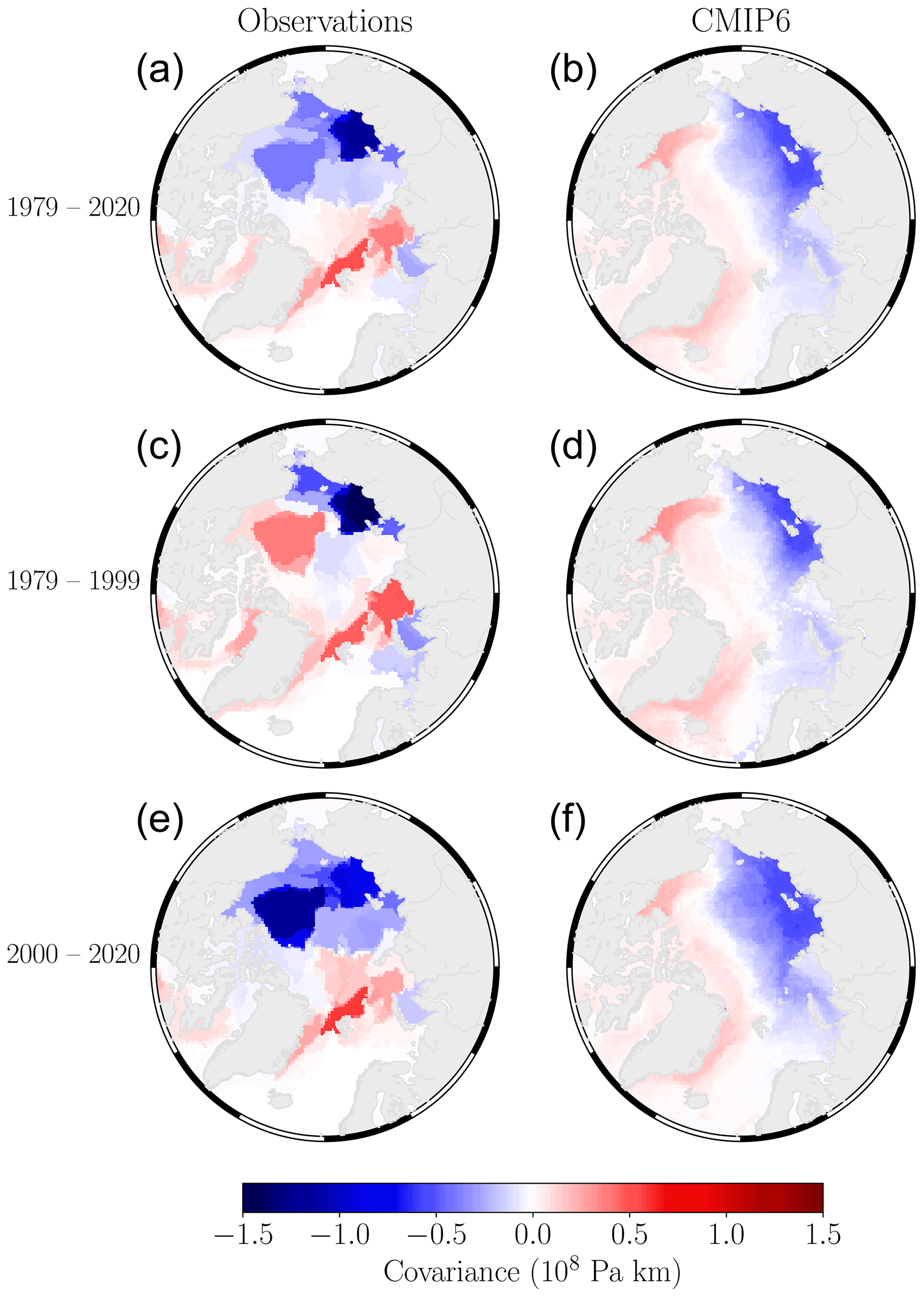
Figure 13The average covariance-based link weights between the winter AO node time series and each node of the summer sea ice concentration networks across both the observations (a, c, e) and all CMIP6 model ensemble members (b, d, f). Each row shows the link weights computed over different parts of the time series record: 1979–2020 (a, b), 1979–1999 (c, d), and 2000–2020 (e, f).
In Fig. 13 we now show the average teleconnection link weights between the winter AO and summer sea ice concentration node time series for both the observations and the average of all CMIP6 ensemble members. Generally, the models agree on the sign of the network links between the winter AO and summer sea ice in the East Siberian and Laptev seas; however the magnitude of this connection is underestimated on average. The models also do not capture the positive connection with the Kara and Barents seas and also do not show the same transition to an overall negative connection in the Eurasian–Pacific sectors between 2000 and 2020. Instead, the Canada Basin region remains moderately positively correlated over the entire record.
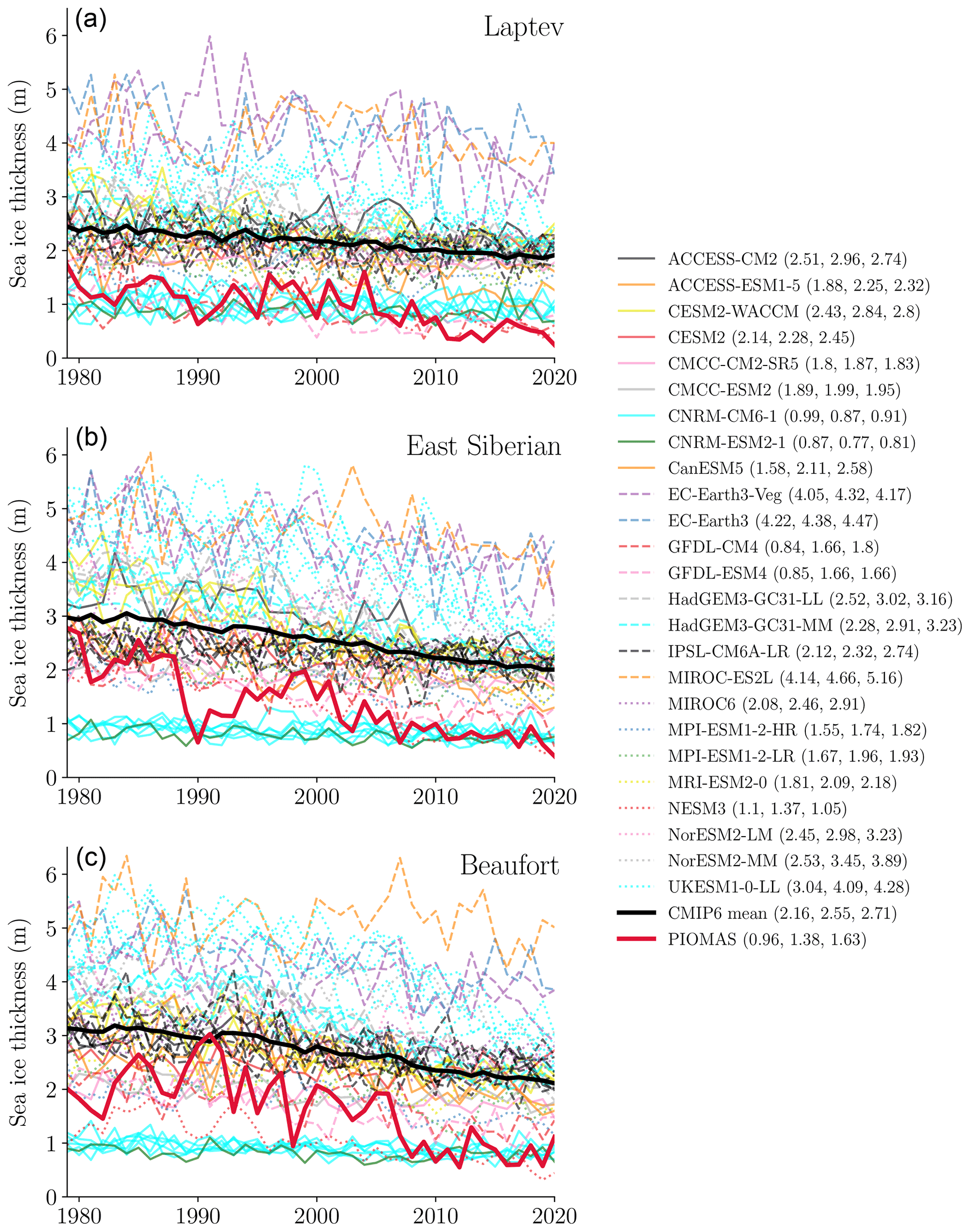
Figure 14The average summer sea ice thickness from 25 CMIP6 models (49 realisations) and PIOMAS in the Laptev Sea (a), East Siberian Sea (b), and Beaufort Sea (c). The numbers in parentheses in the legend are the mean thickness in metres of each respective model (Laptev, East Siberian, Beaufort). For models with multiple ensemble members, the mean thickness time series is computed across all ensemble members, and then the average across 1979–2020 is given.
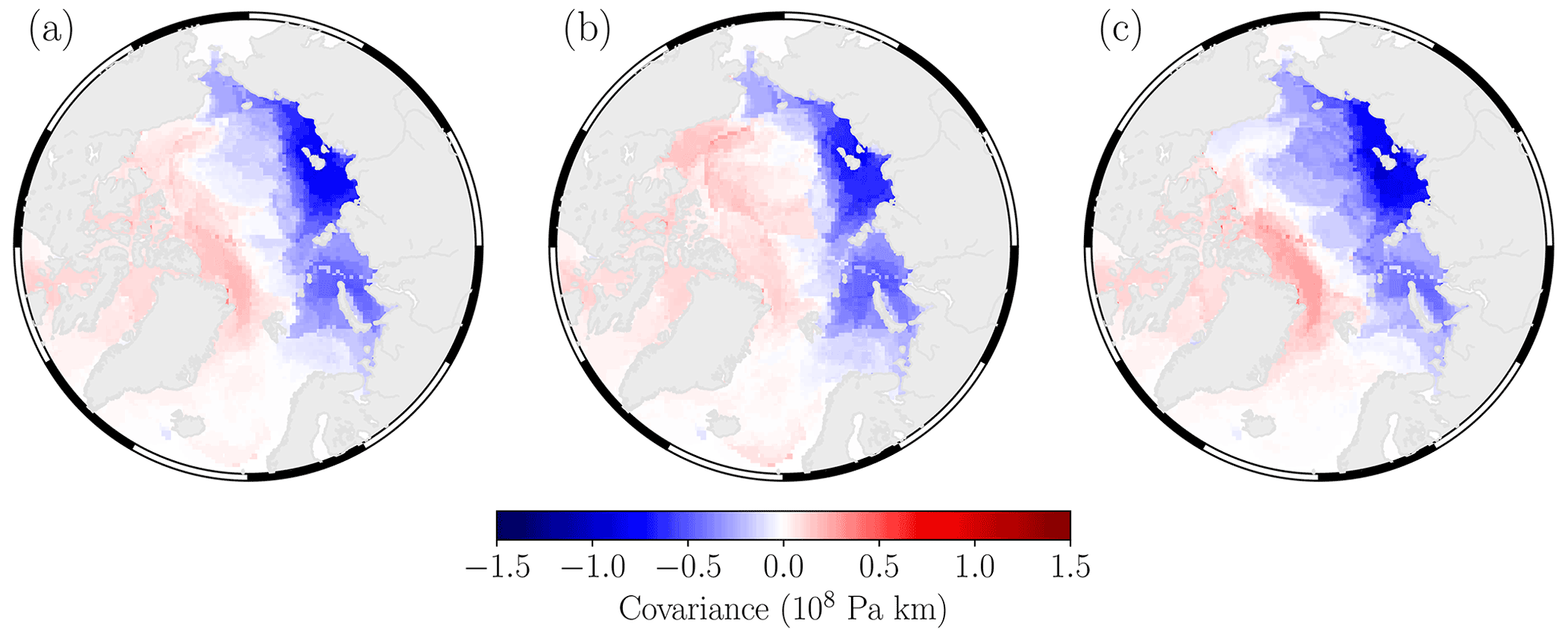
Figure 15Average winter AO to summer sea ice teleconnection for 15 CMIP6 model ensemble members with the lowest average root mean square error (RMSE) in mean sea ice thickness relative to PIOMAS in the East Siberian, Laptev, and Beaufort seas. (a) Links computed between 1979 and 2020, (b) 1979 and 1999, (c) 2000 and 2020.
In this study we used a combination of cluster analysis and complex networks to derive spatio-temporal patterns of variability in Northern Hemisphere winter sea-level pressure and Arctic summer sea ice concentration over the period 1979–2020 and to subsequently understand the spatio-temporal network connectivity between the winter Arctic Oscillation (AO) and summer sea ice cover over the same period. We analysed these patterns in both satellite observational data sets and ERA5 atmospheric reanalysis and also from 31 of the latest generation general circulation models (GCMs) participating in the most recent phase of the Coupled Model Intercomparison Project (CMIP6). We also introduced two global metrics for comparing patterns of variability between two networks: the adjusted Rand index (Hubert and Arabie, 1985) and a network distance metric (Fountalis et al., 2015). Together these allowed us to assess how CMIP6 models perform at replicating the patterns of both winter sea-level pressure and summer sea ice concentration variability relative to ERA5 and the observations, respectively. Previous studies (Rigor et al., 2002; Williams et al., 2016) have suggested a mechanism for the winter AO to summer sea ice teleconnection as follows: a positive winter AO (anomalously low mean sea-level pressure) is coincident with (a) a weakening of the Beaufort Gyre, which reduces the amount of west-to-east ice advection, (b) a strengthening of the Transpolar Drift Stream (TDS), which increases ice export out of the Fram Strait, and (c) an increase in cyclonic ice motion in the Eurasian–Pacific sectors of the Arctic, which causes increased ice divergence and facilitates new winter ice formation. Once the melt season begins, these expanses of relatively thin ice are then more susceptible to melting, thus generally leading to anomalously low sea ice area by the end of summer. We have seen in Fig. 10 that the observations support various aspects of this hypothesis by the fact that the strong negative covariance in the East Siberian Sea means that following a positive winter AO, this region typically sees anomalously low sea ice area in the summer as the ice has undergone thinning and subsequent melting in the spring–summer. The positive covariance in the Fram Strait region suggests that following positive AO winters we see an increase in sea ice in this area which is due to positive AO events strengthening the TDS, resulting in large quantities of ice being advected towards the Atlantic sector (Rigor et al., 2002; Ricker et al., 2018). The fact that we see an overall shift towards more strongly negative covariance between 1979 and 1999 and 2000 and 2020 across the whole Eurasian–Pacific sector is likely due to the significant reductions in the thicker multi-year ice cover that have occurred in this region over recent decades (Maslanik et al., 2007; Kwok, 2018). Between 1979 and 1999 the substantially thicker ice cover in the western Arctic was able to withstand the thinning caused by increased ice divergence from a weakened Beaufort Gyre during positive AO events, thus allowing it to survive through the melt season. More recently, however, a thinner ice cover means areas of open water are more likely to form during the periods of increased ice divergence in the western Arctic, leading to the growth of new ice which is more susceptible to dramatic ice melt throughout the spring–summer. The inability of certain CMIP6 models to accurately reflect the dominant regions of winter sea-level pressure or summer sea ice concentration variability, and their connectivity structure, could be due to a number of factors. While we have seen that internal variability is likely to play a role in governing the magnitude of regional variability in either field for any one model ensemble member, in Fig. 6 we saw that (on average) CMIP6 models replicate the spatial patterns of winter sea-level pressure relatively well (compared to ERA5); however they generally overestimate the magnitude of connectivity over the North Pacific and underestimate the magnitude over the Arctic Ocean and the North Atlantic, consistent with previous analyses of CMIP5 models (Zuo et al., 2013; Gong et al., 2016). A recent study by Gong et al. (2019) suggested that the strong North Pacific pattern of variability in GCMs is likely due to the overestimation of the strength of the stratospheric polar vortex (a persistent feature of models with lower vertical resolutions in their atmospheric components) which causes enhanced coupling of atmospheric circulation between the North Pacific and North Atlantic. In terms of summer sea ice, we have seen in Fig. 9 that, on average, CMIP6 models show discrepancies in the regions which govern summer sea ice variability and that they generally underestimate the contributions from regions such as the Beaufort, East Siberian, and Laptev seas (Pacific sector) in explaining pan-Arctic summer sea ice area variability and similarly overestimate contributions from the Barents Sea and Eurasian Basin (Atlantic sector). The biases in the Atlantic sector are likely related to the models' overestimation of the sea ice extent in these regions as in reality these regions are now largely ice-free in summer (hence the observations show little variability). Meanwhile, biases in the Pacific sector are more likely due to the poor representation of the spatial sea ice thickness distribution in models, which was previously shown to be an issue in CMIP5 models (Stroeve et al., 2014), and also recently for a subset of CMIP6 models (Watts et al., 2021). The sea ice thickness distribution strongly determines how susceptible regions are to melting in the summer (Massonnet et al., 2018) as thicker ice effectively dampens the amount of energy transfer between the atmosphere and ocean. In Fig. 14 we show the average regional summer sea ice thickness in the Beaufort, East Siberian, and Laptev seas from both PIOMAS and 25 of the CMIP6 models used in this study (thickness outputs were not available for BCC-CSM2-MR, CAMS-CSM1-0, CAS-ESM2-0, FGOALS-g3, FIO-ESM-2-0, and CanESM5-CanOE at the time of this study). On average, CMIP6 models report higher average thickness than PIOMAS in each region, which could explain their relatively low contributions to pan-Arctic summer sea ice area variability. The regional biases in sea ice thickness estimates from CMIP6 models could be related to several factors which determine sea ice transport and hence the ice thickness distribution, including biases in surface winds, ice rheology, and ocean heat fluxes (Stroeve et al., 2014; Watts et al., 2021). Given then that positive winter AO events typically act to pre-condition the ice for increased melting (Williams et al., 2016), models which may perhaps reflect the spatio-temporal patterns of winter sea-level pressure variability well may still misrepresent the effects of the winter AO on summer sea ice because the ice is too thick, and subsequently, they therefore underestimate the amount of variability that these sea ice regions explain in terms of pan-Arctic summer sea ice area. To briefly test this hypothesis, Fig. 15 shows the average CMIP6 winter AO to summer sea ice teleconnection (as in Fig. 13), although this time computed only for a subset of 15 model ensemble members (see Table S1) which show the lowest total root mean square error (RMSE) in terms of their mean summer sea ice thickness relative to PIOMAS in the East Siberian, Laptev, and Beaufort seas. Comparing this with Fig. 13, we notice that when only considering the models with thinner regional sea ice, the magnitude of covariance between the winter AO and summer sea ice in the East Siberian and Laptev seas is increased and that between 1979 and 1999 and 2000 and 2020 there is evidence of the Beaufort Sea becoming more negatively correlated although still with a lower magnitude than shown in the observations. Framing these results in the perspective of dynamical sea ice forecasts, the accuracy of seasonal to inter-annual sea ice predictions in GCMs ultimately hinges upon their ability to reproduce the physical processes that drive sea ice variability and subsequently their ability to reflect the geographic regions which are responsible for explaining the overall variability in summer sea ice area. In recent years we have seen the improvement in seasonal predictions brought by initialising dynamical models with observations of sea ice thickness (Chevallier and Salas-Mélia, 2012; Doblas-Reyes et al., 2013; Day et al., 2014; Collow et al., 2015; Bushuk et al., 2017; Allard et al., 2018; Blockley and Peterson, 2018; Schröder et al., 2019; Ono et al., 2020; Balan-Sarojini et al., 2021); therefore reducing sea ice thickness biases in GCMs could be a way to potentially improve the representation of the winter AO to summer sea ice teleconnection in those models. To more accurately determine the specific role of regional sea ice thickness variability in this teleconnection and subsequently isolate the point at which this teleconnection breaks down across CMIP6 models, the methodology here could be advanced to include causal inference principles (e.g. Runge et al., 2019) while also including additional winter–spring and spring–summer climate variables which act as mediators between winter AO events and the eventual response of summer sea ice, ultimately as a way to begin to bridge the gap between perfect-model and operational dynamical sea ice forecasts.
The following repository contains Python code written by William Gregory, which can be used to access and download CMIP6 data volumes, as well as to perform the complex networks analysis of all data types: https://github.com/William-gregory/CMIP6 (last access: 16 February 2022) (DOI: https://doi.org/10.5281/zenodo.6514306, Gregory, 2022). In the same repository are Python codes to produce ARI and distance metrics for the generated networks.
The satellite-derived sea ice concentration data are available from NSIDC and OSI-SAF at the following locations: NASA Team (https://doi.org/10.5067/8GQ8LZQVL0VL, Cavalieri et al., 1996), Bootstrap (https://doi.org/10.5067/7Q8HCCWS4I0R, Comiso, 2017), OSI-450 (https://doi.org/10.15770/EUM_SAF_OSI_0008, OSI-SAF, 2017), and OSI-430b (https://osi-saf.eumetsat.int/products/osi-430-b-complementing-osi-450, last access: 1 June 2021, EUMETSAT Ocean and Sea Ice Satellite Application Facility, 2000).
The ERA5 atmospheric reanalysis data are available from https://doi.org/10.24381/cds.f17050d7 (Hersbach et al., 2019).
PIOMAS sea ice thickness data are available from http://psc.apl.uw.edu/research/projects/arctic-sea-ice-volume-anomaly/data/model_grid (last access: 2 March 2021) (Polar Science Center, 2021).
CMIP6 model ensemble members used in this study were hosted on the JASMIN UK supercomputer; however these same files can be downloaded directly from https://doi.org/10.5281/zenodo.6514306 (Gregory, 2022). See also https://github.com/William-gregory/CMIP6 (last access: 16 February 2022) for more information on bulk downloads of CMIP6 data.
The supplement related to this article is available online at: https://doi.org/10.5194/tc-16-1653-2022-supplement.
WG developed the networks code and subsequently ran the analysis for all the observational, reanalysis, and model data. JS originally suggested the idea of applying the complex networks framework to analysing sea ice teleconnections in CMIP6 models and also provided technical support and input for this paper. MT provided technical support and input for this paper. All co-authors contributed to all sections of the paper.
At least one of the (co-)authors is a member of the editorial board of The Cryosphere. The peer-review process was guided by an independent editor, and the authors also have no other competing interests to declare.
Publisher’s note: Copernicus Publications remains neutral with regard to jurisdictional claims in published maps and institutional affiliations.
Michel Tsamados acknowledges support from the NERC “PRE-MELT” (grant NE/T000546/1) and “EXPRO+ Snow” (ESA AO/1-10061/19/I-EF) projects.
William Gregory received funding from the UK Natural Environment Research Council (NERC) (grant NE/L002485/1).
This paper was edited by Yevgeny Aksenov and reviewed by Céline Gieße and Robin Clancy.
Abe, S. and Suzuki, N.: Complex-network description of seismicity, Nonlin. Processes Geophys., 13, 145–150, https://doi.org/10.5194/npg-13-145-2006, 2006. a
Albert, R. and Barabási, A.-L.: Statistical mechanics of complex networks, Rev. Mod. Phys., 74, 47, https://doi.org/10.1103/RevModPhys.74.47, 2002. a
Allard, R. A., Farrell, S. L., Hebert, D. A., Johnston, W. F., Li, L., Kurtz, N. T., Phelps, M. W., Posey, P. G., Tilling, R., Ridout, A., and Wallcraft, A. J.: Utilizing CryoSat-2 sea ice thickness to initialize a coupled ice-ocean modeling system, Adv. Space Res., 62, 1265–1280, https://doi.org/10.1016/j.asr.2017.12.030, 2018. a
Årthun, M., Onarheim, I. H., Dörr, J., and Eldevik, T.: The seasonal and regional transition to an ice-free Arctic, Geophys. Res. Lett., 48, e2020GL090825, https://doi.org/10.1029/2020GL090825, 2021. a
Balan-Sarojini, B., Tietsche, S., Mayer, M., Balmaseda, M., Zuo, H., de Rosnay, P., Stockdale, T., and Vitart, F.: Year-round impact of winter sea ice thickness observations on seasonal forecasts, The Cryosphere, 15, 325–344, https://doi.org/10.5194/tc-15-325-2021, 2021. a
Blockley, E. W. and Peterson, K. A.: Improving Met Office seasonal predictions of Arctic sea ice using assimilation of CryoSat-2 thickness, The Cryosphere, 12, 3419–3438, https://doi.org/10.5194/tc-12-3419-2018, 2018. a
Boccaletti, S., Latora, V., Moreno, Y., Chavez, M., and Hwang, D.-U.: Complex networks: Structure and dynamics, Phys. Rep., 424, 175–308, https://doi.org/10.1016/j.physrep.2005.10.009, 2006. a
Boccaletti, S., Bianconi, G., Criado, R., Del Genio, C. I., Gómez-Gardenes, J., Romance, M., Sendina-Nadal, I., Wang, Z., and Zanin, M.: The structure and dynamics of multilayer networks, Phys. Rep., 544, 1–122, https://doi.org/10.1016/j.physrep.2014.07.001, 2014. a
Boers, N., Bookhagen, B., Barbosa, H. M. J., Marwan, N., Kurths, J., and Marengo, J. A.: Prediction of extreme floods in the eastern Central Andes based on a complex networks approach, Nat. Commun., 5, 5199, https://doi.org/10.1038/ncomms6199, 2014. a
Bonan, D. and Blanchard-Wrigglesworth, E.: Nonstationary teleconnection between the Pacific Ocean and Arctic sea ice, Geophys. Res. Lett., 47, e2019GL085666, https://doi.org/10.1029/2019GL085666, 2020. a
Bonan, D. B., Bushuk, M., and Winton, M.: A spring barrier for regional predictions of summer Arctic sea ice, Geophys. Res. Lett., 46, 5937–5947, https://doi.org/10.1029/2019GL082947, 2019. a
Bushuk, M. and Giannakis, D.: The seasonality and interannual variability of Arctic sea ice reemergence, J. Climate, 30, 4657–4676, https://doi.org/10.1175/JCLI-D-16-0549.1, 2017. a, b
Bushuk, M., Msadek, R., Winton, M., Vecchi, G. A., Gudgel, R., Rosati, A., and Yang, X.: Skillful regional prediction of Arctic sea ice on seasonal timescales, Geophys. Res. Lett., 44, 4953–4964, https://doi.org/10.1002/2017GL073155, 2017. a
Bushuk, M., Msadek, R., Winton, M., Vecchi, G., Yang, X., Rosati, A., and Gudgel, R.: Regional Arctic sea–ice prediction: Potential versus operational seasonal forecast skill, Clim. Dynam., 52, 2721–2743, https://doi.org/10.1007/s00382-018-4288-y, 2019. a, b
Bushuk, M., Winton, M., Bonan, D. B., Blanchard-Wrigglesworth, E., and Delworth, T. L.: A mechanism for the Arctic sea ice spring predictability barrier, Geophys. Res. Lett., 47, e2020GL088335, https://doi.org/10.1029/2020GL088335, 2020. a
Cattiaux, J. and Cassou, C.: Opposite CMIP3/CMIP5 trends in the wintertime Northern Annular Mode explained by combined local sea ice and remote tropical influences, Geophys. Res. Lett., 40, 3682–3687, https://doi.org/10.1002/grl.50643, 2013. a
Cavalieri, D. J., Parkinson, C. L., Gloersen, P., and Zwally, H. J.: Sea Ice Concentrations from Nimbus-7 SMMR and DMSP SSM/I-SSMIS Passive Microwave Data, Version 1, NASA National Snow and Ice Data Center Distributed Active Archive Center, Boulder, Colorado USA [data set], https://doi.org/10.5067/8GQ8LZQVL0VL, 1996. a, b
Chevallier, M. and Salas-Mélia, D.: The role of sea ice thickness distribution in the Arctic sea ice potential predictability: A diagnostic approach with a coupled GCM, J. Climate, 25, 3025–3038, https://doi.org/10.1175/JCLI-D-11-00209.1, 2012. a
Cohen, J., Screen, J. A., Furtado, J. C., Barlow, M., Whittleston, D., Coumou, D., Francis, J., Dethloff, K., Entekhabi, D., Overland, J., and Jones, J.: Recent Arctic amplification and extreme mid-latitude weather, Nat. Geosci., 7, 627–637, https://doi.org/10.1038/ngeo2234, 2014. a
Cohen, J., Zhang, X., Francis, J., Jung, T., Kwok, R., Overland, J., Ballinger, T., Bhatt, U., Chen, H., Coumou, D., Feldstein, S., Gu, H., Handorf, D., Henderson, G., Ionita, M., Kretschmer, M., Laliberte, F., Lee, S., Linderholm, H. W., Maslowski, W., Peings, Y., Pfeiffer, K., Rigor, I., Semmler, T., Stroeve, J., Taylor, P. C., Vavrus, S., Vihma, T., Wang, S., Wendisch, M., Wu, Y., and Yoon, J.: Divergent consensuses on Arctic amplification influence on midlatitude severe winter weather, Nat. Clim. Change, 10, 20–29, https://doi.org/10.1038/s41558-019-0662-y, 2020. a
Cohen, R. and Havlin, S.: Complex networks: structure, robustness and function, 1st edn., Cambridge University Press, ISBN (Hardback) 978-0-521-84156-6, ISBN (Online) 9780511780356, https://doi.org/10.1017/CBO9780511780356, 2010. a
Collow, T. W., Wang, W., Kumar, A., and Zhang, J.: Improving Arctic sea ice prediction using PIOMAS initial sea ice thickness in a coupled ocean–atmosphere model, Mon. Weather Rev., 143, 4618–4630, https://doi.org/10.1175/MWR-D-15-0097.1, 2015. a
Comiso, J.: Bootstrap Sea Ice Concentrations from Nimbus-7 SMMR and DMSP SSM/I-SSMIS, Version 3, NASA National Snow and Ice Data Center Distributed Active Archive Center, Boulder, Colorado USA [data set], https://doi.org/10.5067/7Q8HCCWS4I0R, 2017. a, b
Comiso, J. C., Meier, W. N., and Gersten, R.: Variability and trends in the Arctic Sea ice cover: Results from different techniques, J. Geophys. Res.-Oceans, 122, 6883–6900, https://doi.org/10.1002/2017JC012768, 2017. a
Crawford, A. D., Horvath, S., Stroeve, J., Balaji, R., and Serreze, M. C.: Modulation of sea ice melt onset and retreat in the Laptev Sea by the timing of snow retreat in the West Siberian Plain, J. Geophys. Res.-Atmos., 123, 8691–8707, https://doi.org/10.1029/2018JD028697, 2018. a
Day, J., Tietsche, S., and Hawkins, E.: Pan-Arctic and regional sea ice predictability: Initialization month dependence, J. Climate, 27, 4371–4390, https://doi.org/10.1175/JCLI-D-13-00614.1, 2014. a, b
delEtoile, J. and Adeli, H.: Graph theory and brain connectivity in Alzheimer’s disease, Neuroscientist, 23, 616–626, https://doi.org/10.1177/1073858417702621, 2017. a
Deser, C., Walsh, J. E., and Timlin, M. S.: Arctic sea ice variability in the context of recent atmospheric circulation trends, J. Climate, 13, 617–633, https://doi.org/10.1175/1520-0442(2000)013<0617:ASIVIT>2.0.CO;2, 2000. a
Dijkstra, H. A., Hernández-García, E., Masoller, C., and Barreiro, M.: Networks in Climate, 1st edn., Cambridge University Press, ISBN (Hardback) 9781107111233, ISBN (Online) 9781316275757, https://doi.org/10.1017/9781316275757, 2019. a
Doblas-Reyes, F. J., García-Serrano, J., Lienert, F., Biescas, A. P., and Rodrigues, L. R.: Seasonal climate predictability and forecasting: status and prospects, WIRES Clim. Change, 4, 245–268, https://doi.org/10.1002/wcc.217, 2013. a
Donges, J. F., Zou, Y., Marwan, N., and Kurths, J.: Complex networks in climate dynamics: Comparing linear and nonlinear network construction methods, Eur. Phys. J.-Spec. Top., 174, 157–179, https://doi.org/10.1140/epjst/e2009-01098-2, 2009. a, b
Donges, J. F., Petrova, I., Loew, A., Marwan, N., and Kurths, J.: How complex climate networks complement eigen techniques for the statistical analysis of climatological data, Clim. Dynam., 45, 2407–2424, https://doi.org/10.1007/s00382-015-2479-3, 2015. a, b
EUMETSAT Ocean and Sea Ice Satellite Application Facility: Global sea ice concentration interim climate data record 2016–onwards (v2.0, 2017), OSI-430-b, OSI SAF FTP server/EUMETSAT Data Center [data set], https://osi-saf.eumetsat.int/products/osi-430-b-complementing-osi-450, (last access: 1 June 2021), 2016. a
Eyring, V., Bony, S., Meehl, G. A., Senior, C. A., Stevens, B., Stouffer, R. J., and Taylor, K. E.: Overview of the Coupled Model Intercomparison Project Phase 6 (CMIP6) experimental design and organization, Geosci. Model Dev., 9, 1937–1958, https://doi.org/10.5194/gmd-9-1937-2016, 2016. a
Fountalis, I., Bracco, A., and Dovrolis, C.: Spatio-temporal network analysis for studying climate patterns, Clim. Dynam., 42, 879–899, https://doi.org/10.1007/s00382-013-1729-5, 2014. a, b, c
Fountalis, I., Bracco, A., and Dovrolis, C.: ENSO in CMIP5 simulations: network connectivity from the recent past to the twenty-third century, Clim. Dynam., 45, 511–538, https://doi.org/10.1007/s00382-014-2412-1, 2015. a, b, c
Francis, J. A., Chan, W., Leathers, D. J., Miller, J. R., and Veron, D. E.: Winter Northern Hemisphere weather patterns remember summer Arctic sea-ice extent, Geophys. Res. Lett., 36, L07503, https://doi.org/10.1029/2009GL037274, 2009. a
Fritz, M., Vonk, J. E., and Lantuit, H.: Collapsing arctic coastlines, Nat. Clim. Change, 7, 6–7, https://doi.org/10.1038/nclimate3188, 2017. a
Gidden, M. J., Riahi, K., Smith, S. J., Fujimori, S., Luderer, G., Kriegler, E., van Vuuren, D. P., van den Berg, M., Feng, L., Klein, D., Calvin, K., Doelman, J. C., Frank, S., Fricko, O., Harmsen, M., Hasegawa, T., Havlik, P., Hilaire, J., Hoesly, R., Horing, J., Popp, A., Stehfest, E., and Takahashi, K.: Global emissions pathways under different socioeconomic scenarios for use in CMIP6: a dataset of harmonized emissions trajectories through the end of the century, Geosci. Model Dev., 12, 1443–1475, https://doi.org/10.5194/gmd-12-1443-2019, 2019. a
Giesse, C., Notz, D., and Baehr, J.: On the origin of discrepancies between observed and simulated memory of Arctic sea ice, Geophys. Res. Lett., 48, e2020GL091784, https://doi.org/10.1029/2020GL091784, 2021. a
Gong, H., Wang, L., Chen, W., Chen, X., and Nath, D.: Biases of the wintertime Arctic Oscillation in CMIP5 models, Environ. Res. Lett., 12, 014001, https://doi.org/10.1088/1748-9326/12/1/014001, 2016. a, b
Gong, H., Wang, L., Chen, W., Wu, R., Zhou, W., Liu, L., Nath, D., and Lan, X.: Diversity of the wintertime Arctic Oscillation pattern among CMIP5 models: Role of the stratospheric polar vortex, J. Climate, 32, 5235–5250, https://doi.org/10.1175/JCLI-D-18-0603.1, 2019. a
Graham, R. M., Cohen, L., Ritzhaupt, N., Segger, B., Graversen, R. G., Rinke, A., Walden, V. P., Granskog, M. A., and Hudson, S. R.: Evaluation of six atmospheric reanalyses over Arctic sea ice from winter to early summer, J. Climate, 32, 4121–4143, https://doi.org/10.1175/JCLI-D-18-0643.1, 2019. a
Gregory, W.: William-gregory/CMIP6: Accompanying code for: “Network connectivity between the winter Arctic Oscillation and summer sea ice in CMIP6 models and observations” (v1.0), Zenodo [code], https://doi.org/10.5281/zenodo.6514306, 2022. a, b
Gregory, W., Tsamados, M., Stroeve, J., and Sollich, P.: Regional September Sea Ice Forecasting with Complex Networks and Gaussian Processes, Weather Forecast., 35, 793–806, https://doi.org/10.1175/WAF-D-19-0107.1, 2020. a, b, c, d
Hawkins, E. and Sutton, R.: The potential to narrow uncertainty in regional climate predictions, B. Am. Meteorol. Soc., 90, 1095–1108, https://doi.org/10.1175/2009BAMS2607.1, 2009. a
Hersbach, H., Bell, B., Berrisford, P., Biavati, G., Horányi, A., Muñoz Sabater, J., Nicolas, J., Peubey, C., Radu, R., Rozum, I., Schepers, D., Simmons, A., Soci, C., Dee, D., and Thépaut, J.-N.: ERA5 monthly averaged data on single levels from 1979 to present, Copernicus Climate Change Service (C3S) Climate Data Store (CDS) [data set], https://doi.org/10.24381/cds.f17050d7, 2019. a, b
Holland, M. M., Bailey, D. A., and Vavrus, S.: Inherent sea ice predictability in the rapidly changing Arctic environment of the Community Climate System Model, version 3, Clim. Dynam., 36, 1239–1253, https://doi.org/10.1007/s00382-010-0792-4, 2011. a
Hubert, L. and Arabie, P.: Comparing partitions, J. Classif., 2, 193–218, https://doi.org/10.1007/BF01908075, 1985. a, b, c
Hurrell, J. W., Kushnir, Y., Ottersen, G., and Visbeck, M.: An overview of the North Atlantic oscillation, in: Geophysical Monograph Series, Volume 134, 1–35, https://doi.org/10.1029/134GM01, 2003. a
Jahn, A.: Reduced probability of ice-free summers for 1.5 ∘C compared to 2 ∘C warming, Nat. Clim. Change, 8, 409–413, https://doi.org/10.1038/s41558-018-0127-8, 2018. a
Kapsch, M.-L., Graversen, R. G., and Tjernström, M.: Springtime atmospheric energy transport and the control of Arctic summer sea-ice extent, Nat. Clim. Change, 3, 744–748, https://doi.org/10.1038/nclimate1884, 2013. a
Kay, J. E., Deser, C., Phillips, A., Mai, A., Hannay, C., Strand, G., Arblaster, J. M., Bates, S., Danabasoglu, G., Edwards, J., Holland, M., Kushner, P., Lamarque, J.-F., Lawrence, D., Lindsay, K., Middleton, A., Munoz, E., Neale, R., Oleson, K., Polvani, L., and Vertenstein, M.: The Community Earth System Model (CESM) large ensemble project: A community resource for studying climate change in the presence of internal climate variability, B. Am. Meteorol. Soc., 96, 1333–1349, https://doi.org/10.1175/BAMS-D-13-00255.1, 2015. a
Kwok, R.: Arctic sea ice thickness, volume, and multiyear ice coverage: losses and coupled variability (1958–2018), Environ. Res. Lett., 13, 105005, https://doi.org/10.1088/1748-9326/aae3ec, 2018. a
Larsen, J. N., Schweitzer, P., Abass, K., Doloisio, N., Gartler, S., Ingeman-Nielsen, T., Ingimundarson, J. H., Jungsberg, L., Meyer, A., Rautio, A., Scheer, J., Timlin, U., Vanderlinden, J.-P., and Vullierme, M.: Thawing permafrost in arctic coastal communities: A framework for studying risks from climate change, Sustainability, 13, 2651, https://doi.org/10.3390/su13052651, 2021. a
Lavergne, T., Sørensen, A. M., Kern, S., Tonboe, R., Notz, D., Aaboe, S., Bell, L., Dybkjær, G., Eastwood, S., Gabarro, C., Heygster, G., Killie, M. A., Brandt Kreiner, M., Lavelle, J., Saldo, R., Sandven, S., and Pedersen, L. T.: Version 2 of the EUMETSAT OSI SAF and ESA CCI sea-ice concentration climate data records, The Cryosphere, 13, 49–78, https://doi.org/10.5194/tc-13-49-2019, 2019. a
Malik, N., Bookhagen, B., Marwan, N., and Kurths, J.: Analysis of spatial and temporal extreme monsoonal rainfall over South Asia using complex networks, Clim. Dynam., 39, 971–987, 2012. a
Mallett, R., Stroeve, J., Cornish, S., Crawford, A., Lukovich, J., Serreze, M., Barrett, A., Meier, W., Heorton, H., and Tsamados, M.: Record winter winds in 2020/21 drove exceptional Arctic sea ice transport, Commun. Earth Environ., 2, 149, https://doi.org/10.1038/s43247-021-00221-8, 2021. a
Maslanik, J., Fowler, C., Stroeve, J., Drobot, S., Zwally, J., Yi, D., and Emery, W.: A younger, thinner Arctic ice cover: Increased potential for rapid, extensive sea-ice loss, Geophys. Res. Lett., 34, L24501, https://doi.org/10.1029/2007GL032043, 2007. a
Maslanik, J. A., Serreze, M. C., and Barry, R. G.: Recent decreases in Arctic summer ice cover and linkages to atmospheric circulation anomalies, Geophys. Res. Lett., 23, 1677–1680, https://doi.org/10.1029/96GL01426, 1996. a
Massonnet, F., Vancoppenolle, M., Goosse, H., Docquier, D., Fichefet, T., and Blanchard-Wrigglesworth, E.: Arctic sea-ice change tied to its mean state through thermodynamic processes, Nat. Clim. Change, 8, 599–603, https://doi.org/10.1038/s41558-018-0204-z, 2018. a
Matsumura, S., Zhang, X., and Yamazaki, K.: Summer Arctic atmospheric circulation response to spring Eurasian snow cover and its possible linkage to accelerated sea ice decrease, J. Climate, 27, 6551–6558, https://doi.org/10.1175/JCLI-D-13-00549.1, 2014. a
Miller, R., Schmidt, G., and Shindell, D.: Forced annular variations in the 20th century intergovernmental panel on climate change fourth assessment report models, J. Geophys. Res.-Atmos., 111, D18101, https://doi.org/10.1029/2005JD006323, 2006. a
Mioduszewski, J. R., Vavrus, S., Wang, M., Holland, M., and Landrum, L.: Past and future interannual variability in Arctic sea ice in coupled climate models, The Cryosphere, 13, 113–124, https://doi.org/10.5194/tc-13-113-2019, 2019. a
Morabito, F. C., Campolo, M., Labate, D., Morabito, G., Bonanno, L., Bramanti, A., De Salvo, S., Marra, A., and Bramanti, P.: A longitudinal EEG study of Alzheimer's disease progression based on a complex network approach, Int. J. Neural Syst., 25, 1550005, https://doi.org/10.1142/S0129065715500057, 2015. a
Newman, M. E.: The structure and function of complex networks, SIAM Rev., 45, 167–256, https://doi.org/10.1137/S003614450342480, 2003. a
Notz, D.: How well must climate models agree with observations?, Philosophical Transactions of the Royal Society A: Mathematical, Physical and Engineering Sciences, 373, 20140164, https://doi.org/10.1098/rsta.2014.0164, 2015. a
Notz, D. and SIMIP-Community: Arctic sea ice in CMIP6, Geophys. Res. Lett., 47, e2019GL086749, https://doi.org/10.1029/2019GL086749, 2020. a
Notz, D. and Stroeve, J.: Observed Arctic sea-ice loss directly follows anthropogenic CO2 emission, Science, 354, 747–750, https://doi.org/10.1126/science.aag2345, 2016. a
Olonscheck, D., Mauritsen, T., and Notz, D.: Arctic sea-ice variability is primarily driven by atmospheric temperature fluctuations, Nat. Geosci., 12, 430–434, https://doi.org/10.1038/s41561-019-0363-1, 2019. a
Onarheim, I. H., Eldevik, T., Smedsrud, L. H., and Stroeve, J. C.: Seasonal and regional manifestation of Arctic sea ice loss, J. Climate, 31, 4917–4932, https://doi.org/10.1175/JCLI-D-17-0427.1, 2018. a
Ono, J., Komuro, Y., and Tatebe, H.: Impact of sea-ice thickness initialized in April on Arctic sea-ice extent predictability with the MIROC climate model, Ann. Glaciol., 61, 97–105, https://doi.org/10.1017/aog.2020.13, 2020. a
OSI-SAF: Global Sea Ice Concentration Climate Data Record v2.0 – Multimission, EUMETSAT SAF on Ocean and Sea Ice [data set], https://doi.org/10.15770/EUM_SAF_OSI_0008, 2017. a, b
Overland, J. E., Francis, J. A., Hanna, E., and Wang, M.: The recent shift in early summer Arctic atmospheric circulation, Geophys. Res. Lett., 39, L19804, https://doi.org/10.1029/2012GL053268, 2012. a
Park, H.-S., Stewart, A. L., and Son, J.-H.: Dynamic and thermodynamic impacts of the winter Arctic Oscillation on summer sea ice extent, J. Climate, 31, 1483–1497, https://doi.org/10.1175/JCLI-D-17-0067.1, 2018. a, b
Polar Science Center: PIOMAS Variables on Model Grid, Polar Science Center [data set], http://psc.apl.uw.edu/research/projects/arctic-sea-ice-volume-anomaly/data/model_grid, last access: 2 March 2021. a
Rand, W. M.: Objective criteria for the evaluation of clustering methods, J. Am. Stat. Assoc., 66, 846–850, https://doi.org/10.1080/01621459.1971.10482356, 1971. a, b
Ricker, R., Girard-Ardhuin, F., Krumpen, T., and Lique, C.: Satellite-derived sea ice export and its impact on Arctic ice mass balance, The Cryosphere, 12, 3017–3032, https://doi.org/10.5194/tc-12-3017-2018, 2018. a
Rigor, I. G., Wallace, J. M., and Colony, R. L.: Response of sea ice to the Arctic Oscillation, J. Climate, 15, 2648–2663, https://doi.org/10.1175/1520-0442(2002)015<2648:ROSITT>2.0.CO;2, 2002. a, b
Runge, J., Nowack, P., Kretschmer, M., Flaxman, S., and Sejdinovic, D.: Detecting and quantifying causal associations in large nonlinear time series datasets, Science Advances, 5, eaau4996, https://doi.org/10.1126/sciadv.aau4996, 2019. a, b
Sakshaug, E., Bjørge, A., Gulliksen, B., Loeng, H., and Mehlum, F.: Structure, biomass distribution, and energetics of the pelagic ecosystem in the Barents Sea: a synopsis, Polar Biol., 14, 405–411, https://doi.org/10.1007/BF00240261, 1994. a
Schröder, D., Feltham, D. L., Flocco, D., and Tsamados, M.: September Arctic sea-ice minimum predicted by spring melt-pond fraction, Nat. Clim. Change, 4, 353–357, https://doi.org/10.1038/nclimate2203, 2014. a
Schröder, D., Feltham, D. L., Tsamados, M., Ridout, A., and Tilling, R.: New insight from CryoSat-2 sea ice thickness for sea ice modelling, The Cryosphere, 13, 125–139, https://doi.org/10.5194/tc-13-125-2019, 2019. a
Schweiger, A., Lindsay, R., Zhang, J., Steele, M., Stern, H., and Kwok, R.: Uncertainty in modeled Arctic sea ice volume, J. Geophys. Res.-Oceans, 116, C00D06, https://doi.org/10.1029/2011JC007084, 2011. a
Serreze, M. C., Maslanik, J. A., Key, J. R., Kokaly, R. F., and Robinson, D. A.: Diagnosis of the record minimum in Arctic sea ice area during 1990 and associated snow cover extremes, Geophys. Res. Lett., 22, 2183–2186, https://doi.org/10.1029/95GL02068, 1995. a
Steinley, D.: Properties of the Hubert-Arable Adjusted Rand Index, Psychol. Methods, 9, 386–396, https://doi.org/10.1037/1082-989X.9.3.386, 2004. a
Stirling, I.: The importance of polynyas, ice edges, and leads to marine mammals and birds, J. Marine Syst., 10, 9–21, https://doi.org/10.1016/S0924-7963(96)00054-1, 1997. a
Stroeve, J. and Notz, D.: Changing state of Arctic sea ice across all seasons, Environ. Res. Lett., 13, 103001, https://doi.org/10.1088/1748-9326/aade56, 2018. a, b
Stroeve, J., Holland, M. M., Meier, W., Scambos, T., and Serreze, M.: Arctic sea ice decline: Faster than forecast, Geophys. Res. Lett., 34, L09501, https://doi.org/10.1029/2007GL029703, 2007. a
Stroeve, J., Barrett, A., Serreze, M., and Schweiger, A.: Using records from submarine, aircraft and satellites to evaluate climate model simulations of Arctic sea ice thickness, The Cryosphere, 8, 1839–1854, https://doi.org/10.5194/tc-8-1839-2014, 2014. a, b, c
Stroeve, J., Vancoppenolle, M., Veyssiere, G., Lebrun, M., Castellani, G., Babin, M., Karcher, M., Landy, J., Liston, G. E., and Wilkinson, J.: A multi-sensor and modeling approach for mapping light under sea ice during the ice-growth season, Frontiers in Marine Science, 7, 592337, https://doi.org/10.3389/fmars.2020.592337, 2021. a
Thompson, D. W. and Wallace, J. M.: The Arctic Oscillation signature in the wintertime geopotential height and temperature fields, Geophys. Res. Lett., 25, 1297–1300, https://doi.org/10.1029/98GL00950, 1998. a, b
Tietsche, S., Day, J. J., Guemas, V., Hurlin, W., Keeley, S., Matei, D., Msadek, R., Collins, M., and Hawkins, E.: Seasonal to interannual Arctic sea ice predictability in current global climate models, Geophys. Res. Lett., 41, 1035–1043, https://doi.org/10.1002/2013GL058755, 2014. a
Tsonis, A. A. and Roebber, P. J.: The architecture of the climate network, Physica A, 333, 497–504, https://doi.org/10.1016/j.physa.2003.10.045, 2004. a, b, c
Tsonis, A. A., Swanson, K. L., and Roebber, P. J.: What do networks have to do with climate?, B. Am. Meteorol. Soc., 87, 585–596, https://doi.org/10.1175/BAMS-87-5-585, 2006. a
Venegas, S. A. and Mysak, L. A.: Is there a dominant timescale of natural climate variability in the Arctic?, J. Climate, 13, 3412–3434, https://doi.org/10.1175/1520-0442(2000)013<3412:ITADTO>2.0.CO;2, 2000. a
Vinje, T.: Anomalies and trends of sea-ice extent and atmospheric circulation in the Nordic Seas during the period 1864–1998, J. Climate, 14, 255–267, https://doi.org/10.1175/1520-0442(2001)014<0255:AATOSI>2.0.CO;2, 2001. a
Watts, M., Maslowski, W., Lee, Y. J., Kinney, J. C., and Osinski, R.: A spatial evaluation of Arctic sea ice and regional limitations in CMIP6 historical simulations, J. Climate, 34, 6399–6420, https://doi.org/10.1175/JCLI-D-20-0491.1, 2021. a, b
Williams, J., Tremblay, B., Newton, R., and Allard, R.: Dynamic preconditioning of the minimum September sea-ice extent, J. Climate, 29, 5879–5891, https://doi.org/10.1175/JCLI-D-15-0515.1, 2016. a, b
Zhang, J. and Rothrock, D.: Modeling global sea ice with a thickness and enthalpy distribution model in generalized curvilinear coordinates, Mon. Weather Rev., 131, 845–861, https://doi.org/10.1175/1520-0493(2003)131<0845:MGSIWA>2.0.CO;2, 2003. a
Zhang, R.: Mechanisms for low-frequency variability of summer Arctic sea ice extent, P. Natl. Acad. Sci., 112, 4570–4575, https://doi.org/10.1073/pnas.1422296112, 2015. a
Zhou, C., Zemanová, L., Zamora-Lopez, G., Hilgetag, C. C., and Kurths, J.: Structure–function relationship in complex brain networks expressed by hierarchical synchronization, New J. Phys., 9, 178, https://doi.org/10.1088/1367-2630/9/6/178, 2007. a
Zuo, J.-Q., Li, W.-J., and Ren, H.-L.: Representation of the Arctic Oscillation in the CMIP5 models, Advances in Climate Change Research, 4, 242–249, https://doi.org/10.3724/SP.J.1248.2013.242, 2013. a, b