The impact of tides on Antarctic ice shelf melting

Tides influence basal melting of individual Antarctic ice shelves, but their net impact on Antarctic-wide ice–ocean interaction has yet to be constrained. Here we quantify the impact of tides on ice shelf melting and the continental shelf seas using a 4 km resolution circum-Antarctic ocean model. Activating tides in the model increases the total basal mass loss by 57 Gt yr⁻¹ (4 %) while decreasing continental shelf temperatures by 0.04 ^∘C. The Ronne Ice Shelf features the highest increase in mass loss (44 Gt yr⁻¹, 128 %), coinciding with strong residual currents and increasing temperatures on the adjacent continental shelf. In some large ice shelves tides strongly affect melting in regions where the ice thickness is of dynamic importance to grounded ice flow. Further, to explore the processes that cause variations in melting we apply dynamical–thermodynamical decomposition to the melt drivers in the boundary layer. In most regions, the impact of tidal currents on the turbulent exchange of heat and salt across the ice–ocean boundary layer has a strong contribution. In some regions, however, mechanisms driven by thermodynamic effects are equally or more important, including under the frontal parts of Ronne Ice Shelf. Our results support the importance of capturing tides for robust modelling of glacier systems and shelf seas, as well as motivate future studies to directly assess friction-based parameterizations for the pan-Antarctic domain.

1 Introduction

Changes in the ocean modulate melting at the base of Antarctic ice shelves, and it is thought that this has consequences for sea-level rise and global climate (e.g. Pritchard et al., 2012; Liu et al., 2015; Bronselaer et al., 2018). The oceanic mechanisms that govern the heat transport across the continental shelf and within sub-ice shelf cavities, however, remain poorly understood and quantified, contributing to large uncertainties in the prediction of future changes (e.g. Asay-Davis et al., 2017; Turner et al., 2017).

One relevant mechanism is ocean tides, which interact with ice shelves in many ways including ice shelf basal melting (Padman et al., 2018). At the ice base, tidal currents enhance the turbulent exchange of heat and salt through the ice–ocean boundary layer and therefore impact local melt rates, as well as meltwater-driven residual flow, which go on to affect ice–ocean interaction downstream (MacAyeal, 1984; Makinson and Nicholls, 1999). Away from the ice shelf base, friction at the sea bed and under static sea ice contributes to ocean mixing (e.g. Padman et al., 2009; Llanillo et al., 2019), as does breaking of internal waves excited by tidally oscillating flow over steep-sloping topography (e.g. Padman et al., 2006; Foldvik et al., 1990). Further, tidal currents can be rectified into a mean flow component (Loder, 1980) with velocity magnitudes comparable to the ambient circulation (Padman et al., 2009; MacAyeal, 1985; Makinson and Nicholls, 1999). By means of these mechanisms, tides are thought to play a fundamental role in the transport of heat across the continental shelf break (Padman et al., 2009; Stewart et al., 2018), vertical mixing and advection at the ice front (Gammelsrod and Slotsvik, 1981; Foldvik et al., 1985; Makinson and Nicholls, 1999), and vertical transport of heat and salt inside sub-ice shelf cavities (MacAyeal, 1984). The roles of these processes for ice-shelf–ocean interaction in an Antarctic-wide context, however, are not well understood, inhibiting reliable parameterizations in large-scale climate simulations (Asay-Davis et al., 2017; Jourdain et al., 2019).

Regional ocean–ice-shelf models that explicitly resolve tides have now been successfully applied to all large ice shelves around Antarctica (e.g. Makinson et al., 2011; Mueller et al., 2012, 2018; Galton‐Fenzi et al., 2012; Robertson, 2013; Arzeno et al., 2014; Mack et al., 2017; Jourdain et al., 2019). The combined domains, however, do not cover all of the Antarctic coastline, neglecting the potentially important contribution of small ice shelves (discussed in, for example, Timmermann et al., 2012) and ice shelf teleconnections (Gwyther et al., 2014; Silvano et al., 2018). Also, inconsistent design and parameter choices make it difficult to identify the governing processes on a continent-wide scale. In contrast, ocean general circulation models (OGCMs) that have global coverage and include tidal currents have not been extended to include an ice shelf component (Savage et al., 2017; Stewart et al., 2018). To our best knowledge, no Antarctic-wide ocean model that resolves ice shelf interactions and tides simultaneously has so-far been developed (Asay-Davis et al., 2017). Here, using an Antarctic-wide ocean–ice-shelf model that explicitly resolves tides, we quantify the impact of tidal currents on ice shelf basal melting and the continental shelf seas. Further, we derive insights into the governing mechanisms that drive tidal melting by performing a dynamical–thermodynamical decomposition of the melt drivers at the ice shelf base (similar to Jourdain et al., 2019).

The following section (Sect. 2) describes the model, experiments and analysis techniques used in this study. Section 3 presents the results. First, we show the effects of tides on annually averaged ice shelf melting and on the oceanographic conditions of the continental shelf seas. Second, we present the outcome of the decomposition analysis. The results section is followed by a discussion of the implications for larger-scale modelling efforts that include ice sheets and global oceans (Sect. 4). The last section (Sect. 5) summarizes the study and presents its conclusions.

2 Methods

2.1 Model description

We derive estimates of ice-shelf–ocean interaction using the Whole Antarctic Ocean Model (WAOM) at 4 km horizontal resolution (Richter et al., 2022). The reference simulation performed for this study is similar to the experiment described and evaluated by Richter et al. (2022) except for the horizontal resolution (Richter et al., 2022, evaluates the 2 km version of the model). At 4 km horizontal resolution, we resolve the tidal processes critical for the focus of this study (as discussed in Richter et al., 2022). In the following we re-state the key points of WAOM and describe the experiments performed here. The model is based on the Regional Ocean Modeling System (ROMS) version 3.6 (Shchepetkin and McWilliams, 2005), which uses terrain-following vertical coordinates and has been augmented by an ice shelf component (Galton‐Fenzi et al., 2012). Thermodynamic ice–ocean interaction is described using the three-equation melt parameterization (Hellmer and Olbers, 1989; Holland and Jenkins, 1999) including velocity-dependent exchange coefficients (McPhee, 1987) and a modification that ensures a weak exchange in the case of zero velocity (due to molecular diffusion; see Gwyther et al., 2016).

The domain covers the entire Antarctic continental shelf, including all ice shelf cavities (as shown in Fig. 1). The bathymetry and ice draft topography have been taken from the Bedmap2 dataset (Fretwell et al., 2013), while boundaries for 139 individual ice shelves are based on the MEaSURES Antarctic boundary dataset (Mouginot et al., 2016). A well-known feature of terrain-following coordinates are pressure gradient errors in regions of steep-sloping topography, ultimately driving spurious circulation patterns (Mellor et al., 1994, 1998). To minimize pressure gradient errors in WAOM, we smooth the ice draft and bottom topography using the Mellor–Ezer–Oey algorithm (Mellor et al., 1994) until a maximum Haney factor of 0.3 is reached (Haney, 1991). Further, we artificially deepen the seafloor to a minimum water column thickness of 20 m to ensure numerical stability (see Schnaase and Timmermann, 2019, for implications). The ocean is discretized using a uniform horizontal grid spacing of 4 km and 31 vertical levels with enhanced resolution towards the surface and seafloor. Running the model for 1 year with 2304 CPUs on 2×8 core Intel Xeon E5-2670 (Sandy Bridge) nodes costs about 7000 CPU hours.

Figure 1 Study area and water column thickness on the continental shelf. Colours show the seafloor depth on the open continental shelf and water column thickness where ice shelves are present. The labels indicate locations referred to in the text with ice sheet regions and tributary glaciers on land, as well as ice shelves and ocean sectors on water. Abbreviations are island (Is.), ice rise (I.R.) and peninsula (P.). Inlet shows model boundaries.

2.2 Simulations

For this study we perform two model simulations with ocean–atmosphere–sea-ice conditions from the year 2007, one with tidal forcing and one without tides. We force the tidal run with 13 major constituents (M2, S2, N2, K2, K1, O1, P1, Q1, MF, MM, M4, MS4, MN4) derived from the global tidal solution TPXO7.2 (Egbert and Erofeeva, 2002) as sea surface height and barotropic currents along the northern boundary of the domain (north of 60^∘ S). In this way we achieve an accuracy in the tidal height signal around the coast of Antarctica that is comparable to available barotropic tide models (assessed in King and Padman, 2005; see Richter et al., 2022, their Table 2). At 10 km horizontal resolution WAOM has a combined root-mean-square error in the complex expression of tides of 20 cm, compared with the continent-wide Antarctic Tide Gauge record (Padman et al., 2020). Evaluating tides at higher resolution would have taken considerably more resources, and we expect the improvement in accuracy with finer grid spacing to be incremental. For more information about the accuracy of WAOM's tides, including the spatial distribution, see Richter et al. (2022).

Open boundary conditions and surface fluxes are identical in both simulations. The ocean outside the model domain is described using the ECCO2 reanalysis (Menemenlis et al., 2008) and includes monthly averages of sea surface height, barotropic and baroclinic velocities, temperature, and salinity. At the surface, daily wind stress is calculated by applying a bulk flux formula to ERA-Interim 10 m winds (Dee et al., 2011). We prescribe daily heat and salt fluxes, which have been derived using satellite sea ice data and heat flux calculations (Tamura et al., 2011). Prescribing surface buoyancy fluxes rather than including a sea ice model ensures accurate surface salt flux location and strength from sea ice polynyas. However, discrepancies between the fluxes that correspond to sea ice formation or reduction and the underlying ocean state can lead to the creation of artificial water masses, which can only be compensated for in part without full sea ice interaction (for further details and discussion see Richter et al., 2022). In addition, a small correction term is added to the heat and salt fluxes to constrain model drift over annual timescales. These corrections are based on the difference between the model's solution of surface temperature and salinity and the monthly estimates from the Southern Ocean State Estimate reanalysis (Mazloff et al., 2010). Furthermore, we ensure that positive salt flux from sea ice formation occurs only when sea surface temperatures are at or below freezing. We do not account for the effect of sea ice on wind stress or include an explicit model of frazil ice (as in, for example, Galton‐Fenzi et al., 2012).

Initial temperatures and salinities are also derived from ECCO2, whereby we extrapolate values under the ice shelves from ice front conditions. The extrapolation has been done along sigma levels and, for the horizontal dimensions, using nearest neighbours in cartesian space. The tidal and non-tidal cases were run separately for 5 years using a 10 km version of the model followed by 2 years at 4 km resolution. By performing parts of the spin-up at lower resolution, we reduce computational costs while still ensuring a quasi-equilibrium of the continental shelf seas (measured using the average basal melt rate for all Antarctic ice shelves; see Richter et al., 2022, their Fig. 2). Annual average and decomposition results were derived from the final year of the 4 km simulations from a relatively low-frequency output (monthly). Mean tidal current speed was based on an additional subsequent high-frequency output (hourly) of a 30 d integration (January) of the tidal case. The different output frequency was used to make the most efficient use of available storage on the supercomputer.

2.3 Analysis

We derive an estimate of mean tidal current speed ($|u{|}_{\mathrm{tide}}$). First, we separate the tidal signal from the two orthogonal barotropic velocity components by means of high-pass filtering (u_b,HP and v_b,HP), and, second, we calculate the velocity magnitude from these filtered components as follows:

$$\begin{array}{}\text{(1)}& |u{|}_{\mathrm{tide}}=\langle \sqrt{u_{\mathrm{b},\mathrm{HP}}^{\mathrm{2}}+v_{\mathrm{b},\mathrm{HP}}^{\mathrm{2}}}{\rangle }_{\mathrm{t}}[\mathrm{m}{\mathrm{s}}^{-\mathrm{1}}].\end{array}$$

The temporal average (subscript t) is taken over 30 d of hourly snapshots. The high-pass filter uses a cut-off frequency of 25 h, which has been shown to effectively separate most of the high-frequency variability associated with tides (Stewart et al., 2018). With 30 d we cover two full spring–neap cycles of the major semidiurnal and diurnal tidal constituents M2, S2, K1 and O1. Tidal currents typically reach a maximum speed of 2 $|u{|}_{\mathrm{tide}}$. We find that the seasonal variation in tidal current speed is typically an order of magnitude smaller than the absolute values (not shown) and, hence, negligible for the purpose of this study.

We perform a dynamical–thermodynamical decomposition to explore the mechanisms that govern tidal melting in our simulation (similar to Jourdain et al., 2019). The main characteristics of ice shelf basal melting as derived from the three-equation melt parameterization (w_b) can be approximated using the covariance of friction velocity (u^*) and thermal driving (T^*, see Holland and Jenkins, 1999):

$$\begin{array}{}\text{(2)}& w_{\mathrm{b}}\left[\mathrm{m}{\mathrm{yr}}^{-\mathrm{1}}\right]\propto u^{*}{T}^{*}\left[\mathrm{m}{\mathrm{s}}^{-\mathrm{1}{}^{\circ }}\mathrm{C}\right]\text{ .}\end{array}$$

The friction velocity controls the exchange rates of heat and salt through the boundary layer and is calculated using the surface quadratic stress:

$$\begin{array}{}\text{(3)}& u^{*}=\sqrt{C_{\mathrm{d}}(u_{\mathrm{top}}^{\mathrm{2}}+v_{\mathrm{top}}^{\mathrm{2}})}\left[\mathrm{m}{\mathrm{s}}^{-\mathrm{1}}\right]\text{ .}\end{array}$$

Here, C_d is a quadratic drag coefficient, and u_top and v_top are the orthogonal velocity components of the uppermost sigma layer. Thermal driving is defined as the difference between the mixed-layer temperature and its freezing point calculated at the pressure of the ice base (see Holland and Jenkins, 1999, their Eq. 32):

$$\begin{array}{}\text{(4)}& T^{*}=T_{\mathrm{M}}-(a{S}_{\mathrm{M}}+b+c{p}_{\mathrm{B}})\left[{}^{\circ }\mathrm{C}\right]\text{ .}\end{array}$$

Here, T_M and S_M are the temperature and salinity in the top model cell (approximately 0.3 to 5.0 m below the ice base; assumed to be in the “mixed layer”), a is the slope of liquidus for seawater (−5.73 ${\mathrm{10}}^{-\mathrm{2}}{}^{\circ }\mathrm{C}{\mathrm{psu}}^{-\mathrm{1}}$), b is the offset of liquidus for seawater (9.39 ${\mathrm{10}}^{-\mathrm{2}}{}^{\circ }\mathrm{C}$), c is the change in freezing temperature with pressure (−7.61 ${\mathrm{10}}^{-\mathrm{4}}{}^{\circ }\mathrm{C}{\mathrm{dbar}}^{-\mathrm{1}}$), and p_B is the pressure at the ice shelf base (in dbar). The approximation of melt rate variability using friction velocity and thermal driving (Eq. 2) allows us to decompose the melt rate difference between the tidal and non-tidal experiment into dynamical and thermodynamical components. First, we define a mean state between the tidal and non-tidal case:

$$\begin{array}{}\text{(5)}& \begin{array}{rl}{u}_{\mathrm{m}}^{*}& =(u_{\mathrm{T}}^{*}+u_{\mathrm{NT}}^{*})/\mathrm{2}\text{ ,}\\ T_{\mathrm{m}}^{*}& =(T_{\mathrm{T}}^{*}+T_{\mathrm{NT}}^{*})/\mathrm{2}\text{ ,}\end{array}\end{array}$$

to then develop differences around the mean state:

$$\begin{array}{}\text{(6)}& \begin{array}{rl}\stackrel{\mathrm{‾}}{w_{\mathrm{b},\mathrm{T}}}& -\stackrel{\mathrm{‾}}{w_{\mathrm{b},\mathrm{NT}}}\propto \\ & \stackrel{\mathrm{‾}}{(u_{\mathrm{m}}^{*}+\mathrm{\Delta }{u}^{*}/\mathrm{2})(T_{\mathrm{m}}^{*}+\mathrm{\Delta }{T}^{*}/\mathrm{2})}\\ & -\stackrel{\mathrm{‾}}{(u_{\mathrm{m}}^{*}-\mathrm{\Delta }{u}^{*}/\mathrm{2})(T_{\mathrm{m}}^{*}-\mathrm{\Delta }{T}^{*}/\mathrm{2})}\\ & =\stackrel{\mathrm{‾}}{u_{\mathrm{m}}^{*}\mathrm{\Delta }{T}^{*}}\text{(thermodynamical)}\\ & +\stackrel{\mathrm{‾}}{T_{\mathrm{m}}^{*}\mathrm{\Delta }{u}^{*}}\text{(dynamical).}\end{array}\end{array}$$

Here, the overbar denotes temporal averaging, and the Δ describes the difference between the tidal (T) and non-tidal run (NT):

$$\begin{array}{}\text{(7)}& \begin{array}{rl}\mathrm{\Delta }{u}^{*}& =u_{\mathrm{T}}^{*}-u_{\mathrm{NT}}^{*}\text{ ,}\\ \mathrm{\Delta }{T}^{*}& =T_{\mathrm{T}}^{*}-T_{\mathrm{NT}}^{*}\text{ .}\end{array}\end{array}$$

We approximate using the mean as this study aims to understand the processes responsible for the difference between the tidal and non-tidal state of the model (see Appendix C for further discussion). We have applied this decomposition to key regions around Antarctica using 1 year of hourly averages. The individual terms offer a priori a good physical interpretation. The thermodynamical component accounts for any tidally induced change in the distribution of temperature within the cavity. This includes changes in heat flux upstream, tidal vertical mixing below the turbulent boundary layer (TBL) and effects of chilled meltwater from tidally induced melting. The dynamical term represents changes in shear-driven turbulent mixing in the three-equation model and, thus, any tidally sourced process that contributes to the speed of water flow in the cavity. This covers shear from tidal currents and tidal residual flow, including changes in buoyancy from tidally induced melting.

3 Results

3.1 Mean changes in ice shelf melting and shelf seas

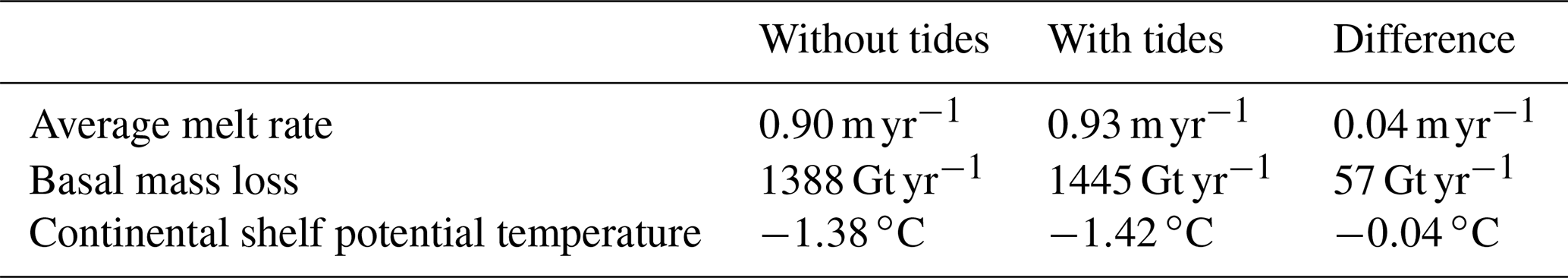
The area-integrated impact of tides on modelled annual-averaged melting and continental shelf sea temperatures is small, as shown in Table 1. The total basal mass loss increases by 4 % when including tides in the model, while ocean temperatures slightly drop (calculated as volume average of the entire ocean south of the 1000 m isobath).

Table 1 Tide-induced difference in area-averaged melt rate, basal mass loss and continental shelf sea temperatures for all Antarctic ice shelves (averaging Figs. 2c and 4). Continental shelf temperatures have been calculated including the sub-ice shelf cavities and using a depth at the shelf break of 1000 m.

The effects of tides on individual ice shelves, however, can be large. Figure 2 presents the spatial distribution of ice shelf melting around Antarctica, as well as the sensitivity of these melt rates to tides. Tides affect melting all around the continent (Fig. 2c) but impact ice shelf integrated mass loss mostly in cold regions where melt rates are typically small (e.g. Filchner, Ronne, Ross and Larsen C ice shelves; Fig. 2b and a). Ronne Ice Shelf shows by far the highest increase in mass loss (44 Gt yr⁻¹, 128 %; see Table A1), only partly compensated for by reduced melting under the adjacent Filchner Ice Shelf (−8 Gt yr⁻¹, −60 %). Melt rate differences within ice shelves are larger. The standard deviation at model resolution, for example, is 352 % (not shown). Areas of increased melting are often close enough to areas of reduced melting or increased marine ice accretion to potentially impact the dynamics of the same ice stream. This net balancing also leads to smaller effects when considering ice shelf area averages.

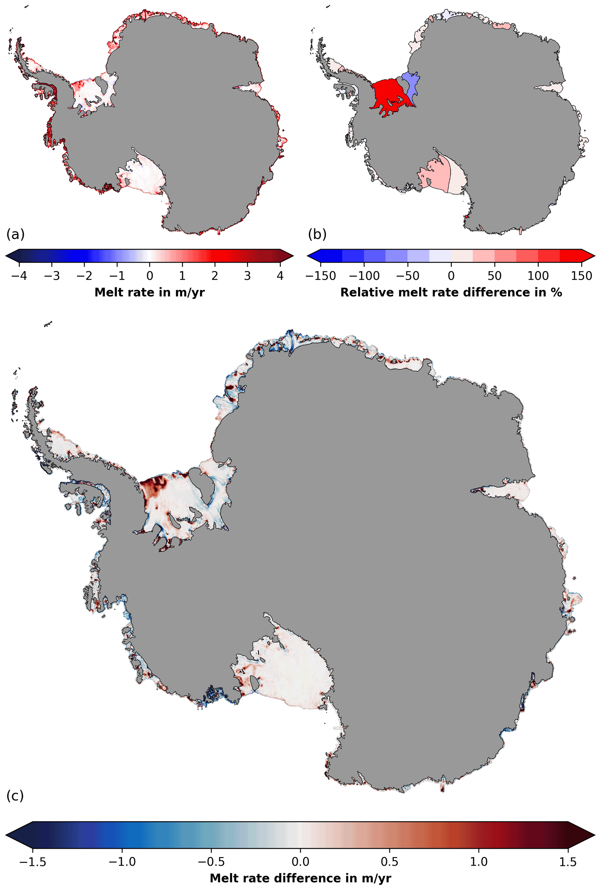
Figure 2 Tidal melting of Antarctic ice shelves. (a) Annual-averaged ice shelf melting for the case with tides, (b) its relative difference to the case without tides averaged over individual ice shelves ($(\text{Tides}-\text{No-Tides})/\text{No-Tides}$) and (c) its absolute difference to the case without tides (Tides−No-Tides).

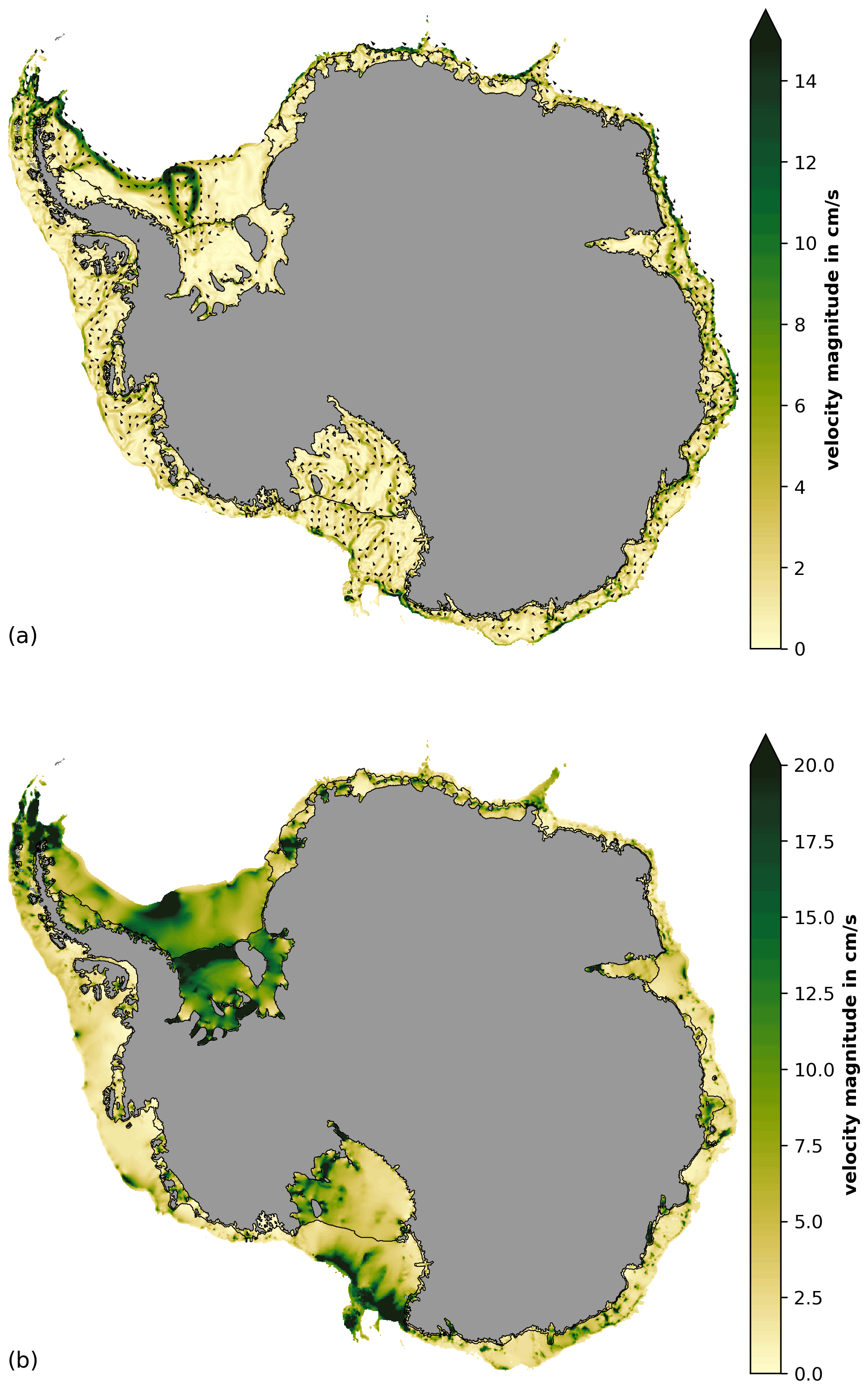
These small-scale impacts can often be linked to local tidal current strength. Figure 3 shows the barotropic currents associated with tides. These currents combine the annual mean circulation (Fig. 3a) and the mean tidal current strength (Fig. 3b; calculated following Eq. 1; see Sect. 2.3). The sub-ice shelf cavities can be very narrow where ice streams drain into the large cold water ice shelves, for example, near Evans Ice Stream, Carlson Inlet and Rutford Ice Stream under Ronne Ice Shelf, near Lambert Glacier under Amery Ice Shelf and near Scott Glacier under Ross Ice Shelf (as shown in Fig. 1). Tidal currents are stronger in these thin water columns near grounding lines (Fig. 3b) and often act to strengthen the ice pump mechanism (Lewis and Perkin, 1986) with enhanced melting at depth followed by reduced melt rates (or increased refreezing) along western outflow regions (Fig. 2c). A similar pattern is also apparent under Fimbul Ice Shelf, where a melt rate increase near the grounding line of the Jutulstraumen Glacier coincides with reduced melt rates all along its keel (Fig. 2c). We note that we artificially deepened the bathymetry in narrow grounding zones, and all of the regions mentioned above are affected by this procedure (see Sect. 2.1). We also note that peaks in tidal velocity away from the grounding zones are often associated with localized melt rate increases, for example, under Riiser-Larsen Ice Shelf and the ice shelves of Queen Maud Land but also in the Amundsen–Bellingshausen seas under the Getz, Abbot and Bach ice shelves.

Figure 4a shows the sensitivity of the mean circulation to tides. This estimate is very similar to the mean circulation of an additional experiment without thermodynamic forcing (see Appendix D), confirming that tide–topography interaction is the main contributor to tidal residual flow (suggested by Robinson, 1981; see also Makinson and Nicholls, 1999). The largest impact on ice shelf integrated mass loss (Ronne Ice Shelf) coincides with the most pronounced feature of tidal residual flow in our simulation. When activating tides in the model, a strong gyre forms on the Weddell Sea continental shelf featuring mean velocities of up to tens of centimetre per second (Fig. 3a) and temperature differences of up to half a degree Celsius (Fig. 4b). This phenomenon has been attributed to tide–topography interaction over Belgrano Bank (Makinson and Nicholls, 1999). Within the sub-ice shelf cavities, residual flow strength is typically an order of magnitude weaker than tidal currents and, hence, can only potentially play a role in tidal melting via transport of heat and salt. The potential contribution of the tidal gyre to the coherent melt increase when activating tides under the northwestern part of Ronne Ice Shelf (Fig. 2c) is discussed later.

Figure 3 Mean and tidal current speed. (a) Mean barotropic velocities from the simulation with tides. (b) Mean speed of oscillating tidal currents ($|u{|}_{\mathrm{tide}}$, calculated following Eq. 1; see Sect. 2.3). Arrows in (a) indicate flow direction and are shown only where velocities are stronger than 1 cm s⁻¹.

Melting in the frontal parts of ice shelves is often associated with local tidal activity. While our results indicate strong melting at the ice shelf front all around the continent (see Fig. 2a; discussed by Richter et al., 2022), in most regions this melting is independent of tides (that is, not coinciding with an equally strong increase in melting due to tides; shown in Fig. 2c). Only at a few places do tides contribute substantially to melting near ice fronts, for example, west of Berkner Island, east of Ross Island and under the Mertz Glacier tongue. Figure 4 shows the sensitivity of depth-averaged continental shelf sea temperatures to tides, and, in the regions mentioned, temperatures adjacent to ice fronts do not show significant warming. Hence, we attribute observed near-ice front melting at these locations to tidal advection of solar heated surface waters (proposed by Jacobs et al., 1992; see, for example, Stewart et al., 2019, for observational evidence).

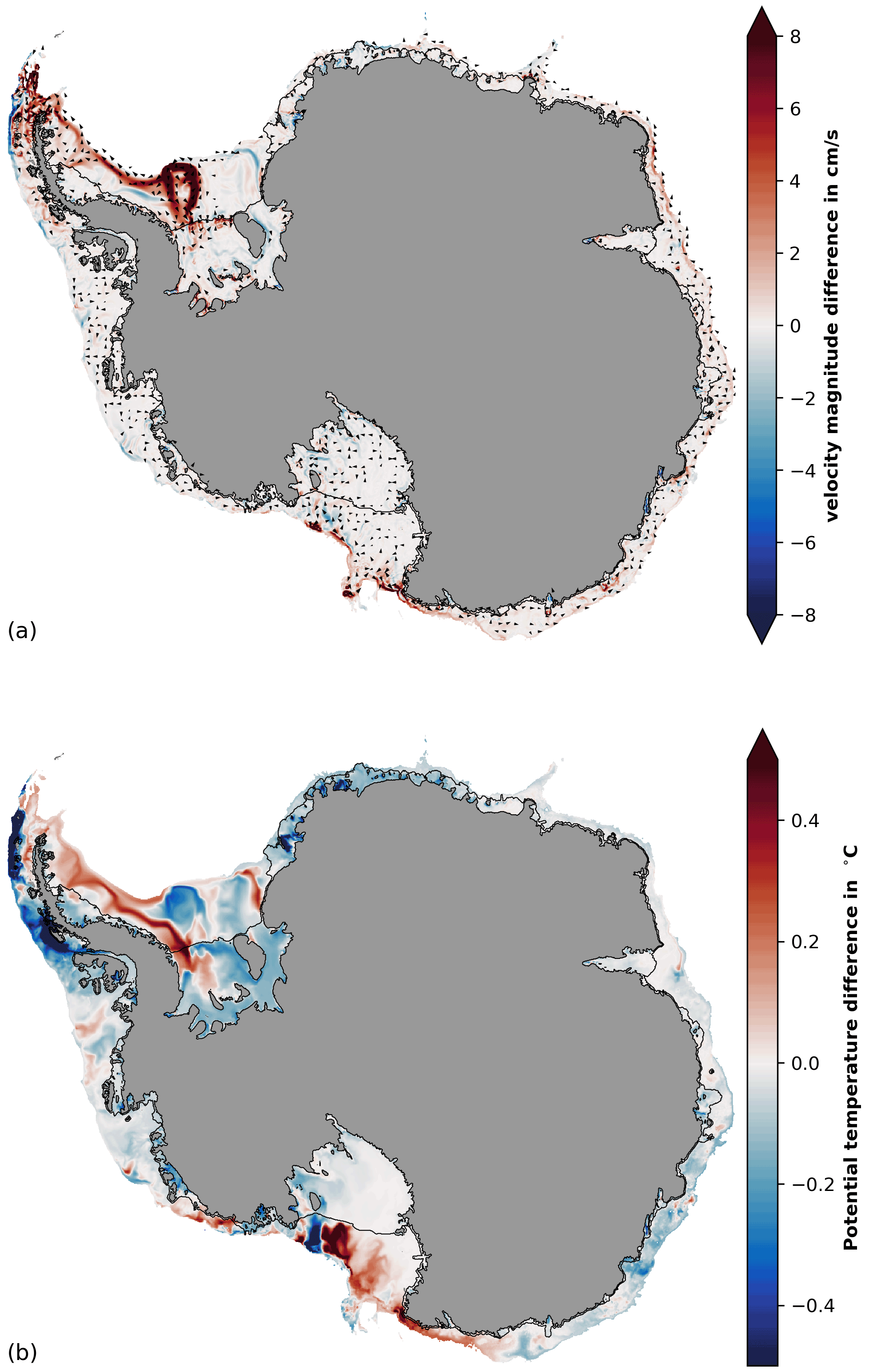
Figure 4 Tide-induced change in (a) magnitude and direction of the depth-averaged velocity vector and (b) depth-averaged potential temperature. Differences show the impact when activating tides in the model (Tides−No-Tides). Arrows in (a) are shown only where velocity change is larger than 1 cm s⁻¹. Panel (a) is very similar to residual flow due to tide–topography interaction alone (see Fig. D1).

3.2 Dynamical–thermodynamical decomposition of tidal melting

We have decomposed the mean impact of tides on ice shelf basal melting into dynamical and thermodynamical parts (see Sect. 2.3). Figures 5 and 6, respectively, show the results of this decomposition for some key regions, organized into regimes with and without signs of relatively warm circumpolar deep water (CDW) intrusions (hereafter referred to as warm and cold regimes). The results for other regions of interest are presented in the Appendix as Figs. B1 and B2.

Figure 5 Dynamical–thermodynamical decomposition of tidal melting in cold regimes. Difference in melting when accounting for all components, only the dynamical component and only the thermodynamical component for Filchner–Ronne (a–c), Ross (d–f), Larsen C (g–i), and Jelbart and Fimbul ice shelves (j–l; following Eq. 6).

Figure 6 Dynamical–thermodynamical decomposition of tidal melting in warm regimes. Difference in melting when accounting for all components, only the dynamical component and only the thermodynamical component for the ice shelves of the Amundsen (a–c) and Bellingshausen seas (d–f; following Eq. 6).

In most regions, dynamical effects have a major positive contribution to melting or refreezing. Tidal currents, for example, increases melting at shallow grounding zones of cold water ice shelves, in agreement with earlier arguments around the ice pump amplification (e.g. under Filchner–Ronne Ice Shelf, along the Siple Coast under Ross Ice Shelf and under Larsen C Ice Shelf, Fig. 5b, e and h, as well as under the Amery Ice Shelf, Fig. B1b). In warm regimes dynamic effects are more pronounced at the trunk of ice shelves (e.g. under Dotson and eastern Getz ice shelves or under Bach and Abbot ice shelves, Fig. 6b and e). Generally, where tidal currents are weak, dynamical tidal melting is also less strong (e.g. under the western half of Ross Ice Shelf, in trunk regions of Filchner–Ronne, Amery, and Larsen C ice shelves, and under Pine Island and Thwaites Ice Shelf).

The thermodynamical contribution often opposes dynamical effects (see, for example, Siple Coast under Ross Ice Shelf and Larsen C Ice Shelf, Fig. 5f and i, as well as Dotson and eastern Getz ice shelves, Fig. 6c). This contrasting behaviour can be explained by the effects of glacial meltwater input resulting from the dynamical contribution of the tides. In melting regions, dynamically enhanced TBL transport causes heat loss in the uppermost ocean layer and, consequently, reduces thermal driving. In regions of marine ice accretion, the effect is reversed.

In some regions, however, melt rate contributions do not follow this pattern. For example, under large parts of northwest Ronne Ice Shelf or under the western half of Getz Ice Shelf the thermodynamical and dynamical terms are both positive. Further, a thermodynamically driven reduction in melt which exceeds dynamic effects is apparent under large parts of Pine Island and Thwaites ice shelves, under eastern George V Ice Shelf (Fig. 6f), and within deeper parts of the cavities under Fimbul (Fig. 5l), Mertz, and Shackleton (Fig. B1f and i) ice shelves, as well as the Totten–Moscow University ice shelf system (Fig. B2c). In such regions, thermodynamical contributions can not be explained as a dynamical consequence alone. Here, some insights into the thermodynamic drivers can be derived considering tide-induced temperature change (Fig. 4b). Coherent changes in continental shelf temperature, for example warming in front of northwest Ronne and western Getz ice shelves or cooling of the eastern Bellingshausen Sea, indicate that tidal impacts on upstream heat flux play an important role. These heat flux differences could take place across the continental shelf break or the ocean surface (as a result of our surface temperature restoring scheme). In contrast, some parts of, for example, Jelbart (Fig. 5l), Totten, Riiser-Larsen, Nickerson (Fig. B2c, f and i), Mertz and Shackleton (Fig. B1f and i) ice shelves exhibit a strong thermodynamic reduction in melt and a cooling that is confined to these parts within the cavity. This signature is likely related to tidal vertical mixing that lifts heat into contact with the ice and consequently cools the water column though meltwater production.

4 Discussion

While the impact of tides on circum-Antarctic total melt is small, regional changes in ice shelf melting and continental shelf temperature can be large (up to orders of magnitude and half a degree Celsius, respectively) with potential implications for ice sheet dynamics and Antarctic Bottom Water formation. The buttressing importance of floating ice can vary by several orders of magnitude within one ice shelf, with regions close to grounding lines, lateral boundaries or pinning points generally being the most important for ice sheet stability (Gudmundsson, 2013; Reese et al., 2018). Our model predicts that the strongest changes in basal mass loss driven by tides often occur in exactly these parts of the ice shelves. Within these regions, however, increased melting is often in close vicinity to equally strong reduction in melting or enhanced refreezing, making it difficult to assess the overall impact on buttressing. Diagnostic experiments with ice sheet flow models could be used to quantify the instantaneous response of tide-driven ice shelf thinning on the ice flux across the grounding lines (similar to experiments by Reese et al., 2018).

Longer-term consequences will be more difficult to assess. Antarctic tides are sensitive to changes in ice shelf geometry and sea levels, offering potential feedback on ice-sheet-relevant timescales. Antarctic tides can be interpreted as waves that propagate around the continent, and barotropic ocean models show that shifts in sea levels, grounding line location and ice draft depth significantly alters their propagation and dissipation (Griffiths and Peltier, 2009; Rosier et al., 2014; Wilmes and Green, 2014). Ice shelf retreat in simulations by Rosier et al. (2014), for example, produces an overall increase in M2 dissipation by more than 40 % (see their Table 1). In our simulation, tides act to slightly increase the overall efficiency of the use of ocean heat for ice shelf melting, a finding supported by idealized simulations by Gwyther et al. (2016). How this conversion efficiency responds to stronger tides is unknown. On a more regional scale, tidal current strength is very sensitive to local changes in the water column thickness, which is set by ice shelf geometry and ocean depth (e.g. Galton-Fenzi et al., 2008; Mueller et al., 2012). Mueller et al. (2018) revealed that slight changes in the draft of Filchner–Ronne Ice Shelf impacts tide-driven melting in areas relevant for inland ice sheet dynamics. Therefore, potential positive and negative feedback between ice geometry, basal melting, and local and also far-field tides will need to be explored using coupled ocean–ice-shelf–ice-sheet models with Antarctic-wide coverage.

Likewise, regional changes in coastal hydrography due to tides might impact water mass transformation with consequences for global oceans and climate. Brine rejection in sea ice polynyas drives the formation of dense water, which has been linked to Antarctic Bottom Water (Purkey and Johnson, 2013) and the meridional overturning circulation (Jacobs, 2004, e.g.). Deep water formation seems to be sensitive to local changes in the ocean as recent studies show that glacial meltwater can offset the densification by polynya activity (Williams et al., 2016; Silvano et al., 2018). Activating tides in our model changes depth-averaged temperatures by up to half a degree Celsius in some locations and generates rectified currents with velocities of up to tens of centimetres per second. The relevance of tide-driven currents and temperature changes for water mass formation and transformation on the Antarctic continental shelf, and indeed on the global oceans and climate, is yet to be explored.

Tides are understood to be critically important for ocean–ice-shelf interaction (e.g. Galton‐Fenzi et al., 2012; Padman et al., 2018), but explicitly resolving tides in larger-scale models is expensive. Hence, several studies have developed or applied parameterizations of tidal melting (see, for example, Jenkins et al., 2010; Hattermann et al., 2014; Asay-Davis et al., 2016; Jourdain et al., 2019). Jourdain et al. (2019) account for tide-driven changes in modelled melting of the Amundsen Sea ice shelves by adding a tidal component to the description of the friction velocity (following Jenkins et al., 2010; similar to enhancing bottom drag in non-tide-resolving estuary models). Using this approach, they reproduce not only the dynamical but also the thermodynamical effects of tides on melting, showing that the latter is a consequence of changes in meltwater input from friction effects in their simulation. In our study, the dynamical component also plays an important role in most regions, and thermodynamical effects in these regions can, to a large degree, be explained as a dynamical consequence (see Figs. 5 and 6).

In some regions, however, thermodynamic drivers govern the melt change. In particular, we have attributed the coherent melt increase under northwest Ronne Ice Shelf to temperature differences outside the TBL. These changes might originate from an ocean warming that spans the ice shelf front, associated with a tide–topography gyre on the adjacent continental shelf (Fig. 4). However, tidal vertical mixing (below the TBL) is also known to be strong here (see Makinson and Nicholls, 1999; in agreement with our tidal current strength, Fig. 3). The strength of the gyre is very uncertain (Makinson and Nicholls, 1999), and a warm bias in WAOM might overestimate its importance for melting. We suggest further investigations are required into the role of the gyre for Filchner–Ronne Ice Shelf melting using a regional model, e.g. based on the ROMS configuration developed by Mueller et al. (2018) with northern boundaries extended up to the continental shelf break. Further, we have identified several regions where tidal vertical mixing below the TBL offers the best explanation for the resolved changes. Any melt rate difference that is indeed induced by the gyre or tidal mixing will not be captured by accounting for dynamical tidal effects on the TBL alone. Overall, the results from this study motivate a direct assessment of the tidal melt parameterization described by Jourdain et al. (2019) in a pan-Antarctic context. WAOM would be well suited to perform these experiments.

The major limitation of this study has its roots in the early development stage of the underlying ocean model. WAOM v1.0 qualitatively reproduces the large-scale characteristics of Antarctic ice-shelf–ocean interaction, but biases have also been identified (Richter et al., 2022), limiting the quantitative conclusions that can be drawn regarding the tidal sensitivity. A warm bias on the western Weddell Sea continental shelf, for example, might lead to an overestimation of the here-reported tide-driven melting under northwest Ronne Ice Shelf (see Richter et al., 2022, their Fig. 9). Likewise, a cold bias on the Amundsen–Bellingshausen seas continental shelf potentially leads to an overestimation of tidal melting driven by thermodynamic effects in this region. Further, sea ice interacts with ice shelf melting (e.g. Hellmer, 2004; Silvano et al., 2018) and tides (Padman et al., 2018), and our approach does not account for these interactions, potentially missing important feedbacks. In the light of these limitations, this study should be seen as a first large-scale investigation into a process potentially important for sea level rise and global climate.

Future studies that aim to apply WAOM, for example to past or future periods, should calibrate vertical tidal mixing first. The tide-induced changes in continental shelf temperature (Fig. 4b) show some similarity with the reported biases (Richter et al., 2022, their Fig. 9), hinting at a connection. Richter et al. (2022) have also identified overly mixed conditions on the continental shelf and linked these to the temperature biases (via erosion of warm deep water in the Amundsen Sea and missing high-salinity shelf water (HSSW) formation in the Weddell Sea). Tidal mixing is sensitive to the choice of the vertical mixing parameterization in ROMS. Our configuration has been tuned by Galton-Fenzi (2009) and used in several regional studies (Galton‐Fenzi et al., 2012; Cougnon et al., 2013; Gwyther et al., 2014). However, there is evidence that the applied mixing scheme (KPP) overestimates tidal vertical mixing (Robertson and Dong, 2019; Robertson, 2006).

5 Summary and conclusion

This study provides a first estimate of tide-driven ice shelf basal melting in an Antarctic-wide context. Activating tides in the model increases total mass loss by 4 %, and mass loss differences for most ice shelves are below 10 %. Filchner–Ronne Ice Shelf exhibits larger coherent changes (Ronne melt increases by 128 %), potentially related to a strong tide-induced gyre over Belgrano Bank. The impact on melt rates at smaller scales can exceed 100 % in cold regimes and are in part located near grounding lines and lateral boundaries, regions important for ice shelf buttressing. The ocean temperature of the entire continental shelf decreases by only 0.04 ^∘C. Regional differences can exceed 0.5 ^∘C including a strong warming of the western Weddell Sea.

Dynamical–thermodynamical decomposition of tidal melting highlights the importance of tidal current enhanced exchange rates of heat and salt in the turbulent boundary layer. This motivates future studies to assess available tidal melt parameterizations (e.g. by Jourdain et al., 2019) in the pan-Antarctic domain. Thermodynamically driven changes due to mixing or residual flow play a role in some regions, but the importance of residual flow might be overestimated due to biases in the control run.

The strong regional sensitivity of ice shelf melting and continental shelf temperatures in our simulation highlights the need to investigate the impact of tides on ice sheet dynamics and Antarctic Bottom Water formation over glacial timescales.

Appendix A: Tide-driven ice shelf basal mass loss

Table A1 Ice shelf average mass loss due to tides. For 139 individual ice shelves the table shows the area, melt rate (w_b) and basal mass loss (BML) of the run with tides, as well as its difference to the run without tides in absolute (e.g. w_b tides−w_b no-tides) and relative ($(w_{\mathrm{b}\text{tides}}-w_{\mathrm{b}\text{no-tides}})/w_{\mathrm{b}\text{no-tides}}$) terms. Ice shelf boundaries have been taken from the MEaSURES dataset (Mouginot et al., 2016).

Appendix B: Dynamical–thermodynamical decomposition for other regions

Figure B1 Dynamical–thermodynamical decomposition of tidal melting under Amery (a–c), Mertz (d–f) and Shackleton (g–i) ice shelves; see Sect. 2.3.

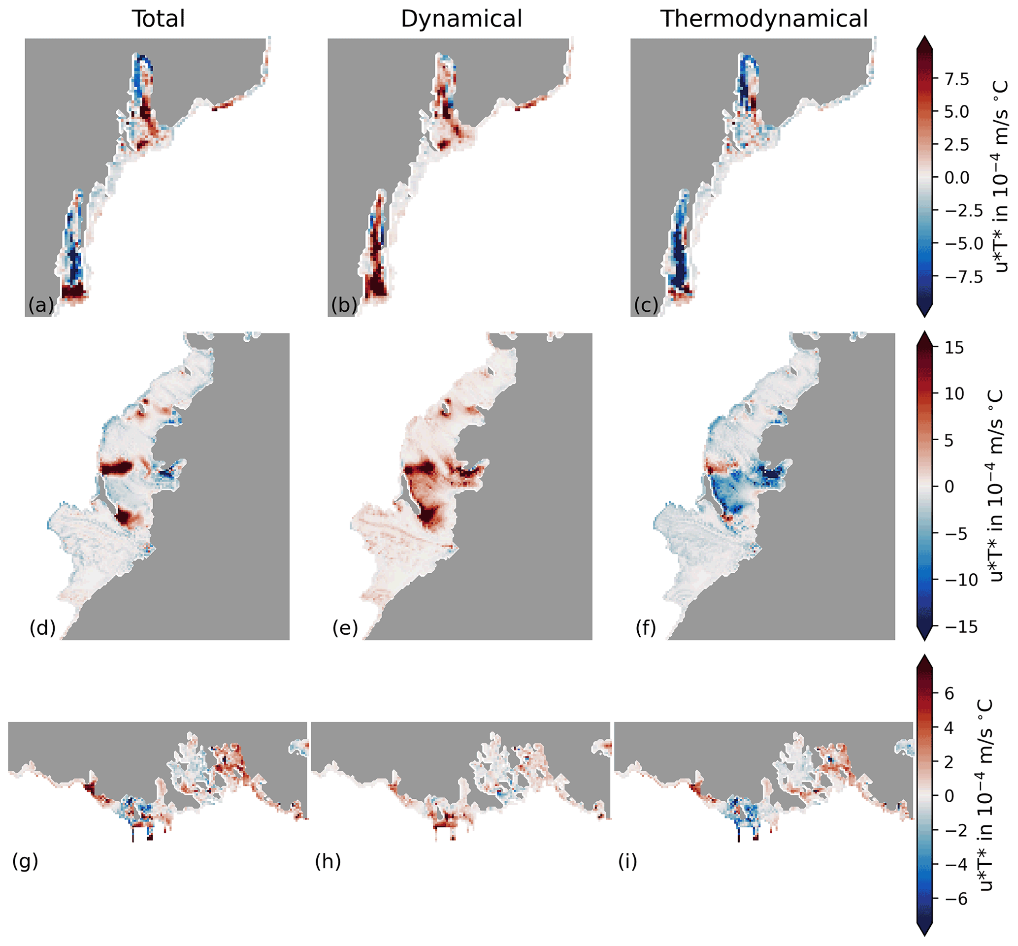
Figure B2 Dynamical–thermodynamical decomposition of tidal melting under the Totten–Moscow University ice shelf system (a–c), Riiser-Larsen Ice Shelf (d–f) and the ice shelves of the eastern Ross Sea (g–i; see Sect. 2.3).

Appendix C: The importance of the reference state for the dynamical–thermodynamical decomposition

The results of the dynamical–thermodynamical decomposition are sensitive to the choice of the reference state. With our experiments, three different approaches can be considered. Approach 1 uses the non-tidal case as reference:

$$\begin{array}{}\text{(C1)}& \begin{array}{rlr}& \stackrel{\mathrm{‾}}{w_{\mathrm{b},\mathrm{T}}}-\stackrel{\mathrm{‾}}{w_{\mathrm{b},\mathrm{NT}}}\propto & \\ & \stackrel{\mathrm{‾}}{u_{\mathrm{NT}}^{*}\mathrm{\Delta }{T}^{*}}& \text{(thermodynamical)}\\ & +\stackrel{\mathrm{‾}}{T_{\mathrm{NT}}^{*}\mathrm{\Delta }{u}^{*}}& \text{(dynamical)}\\ & +\stackrel{\mathrm{‾}}{\mathrm{\Delta }{u}^{*}\mathrm{\Delta }{T}^{*}}& \text{(covariational).}\end{array}\end{array}$$

Approach 2 uses the tidal case as reference:

$$\begin{array}{}\text{(C2)}& \begin{array}{rlr}& \stackrel{\mathrm{‾}}{w_{\mathrm{b},\mathrm{T}}}-\stackrel{\mathrm{‾}}{w_{\mathrm{b},\mathrm{NT}}}\propto & \\ & \stackrel{\mathrm{‾}}{u_{\mathrm{T}}^{*}\mathrm{\Delta }{T}^{*}}& \text{(thermodynamical)}\\ & +\stackrel{\mathrm{‾}}{T_{\mathrm{T}}^{*}\mathrm{\Delta }{u}^{*}}& \text{(dynamical)}\\ & +\stackrel{\mathrm{‾}}{\mathrm{\Delta }{u}^{*}\mathrm{\Delta }{T}^{*}}& \text{(covariational).}\end{array}\end{array}$$

In Approach 3 we define a mean state between the tidal and the non-tidal case:

$$\begin{array}{}\text{(C3)}& \begin{array}{rl}& u_{\mathrm{m}}^{*}=(u_{\mathrm{T}}^{*}+u_{\mathrm{NT}}^{*})/\mathrm{2}\text{ ,}\\ & T_{\mathrm{m}}^{*}=(T_{\mathrm{T}}^{*}+T_{\mathrm{NT}}^{*})/\mathrm{2}\text{ ,}\end{array}\end{array}$$

and develop the difference around this mean state:

$$\begin{array}{}\text{(C4)}& \begin{array}{rl}\stackrel{\mathrm{‾}}{w_{\mathrm{b},\mathrm{T}}}& -\stackrel{\mathrm{‾}}{w_{\mathrm{b},\mathrm{NT}}}\propto \\ & \stackrel{\mathrm{‾}}{(u_{\mathrm{m}}^{*}+\mathrm{\Delta }{u}^{*}/\mathrm{2})(T_{\mathrm{m}}^{*}+\mathrm{\Delta }{T}^{*}/\mathrm{2})}\\ & -\stackrel{\mathrm{‾}}{(u_{\mathrm{m}}^{*}-\mathrm{\Delta }{u}^{*}/\mathrm{2})(T_{\mathrm{m}}^{*}-\mathrm{\Delta }{T}^{*}/\mathrm{2})}\\ & =\stackrel{\mathrm{‾}}{u_{\mathrm{m}}^{*}\mathrm{\Delta }{T}^{*}}\text{(thermodynamical)}\\ & +\stackrel{\mathrm{‾}}{T_{\mathrm{m}}^{*}\mathrm{\Delta }{u}^{*}}\text{(dynamical).}\end{array}\end{array}$$

In each case

$$\begin{array}{}\text{(C5)}& \begin{array}{rl}\mathrm{\Delta }{u}^{*}& =u_{\mathrm{T}}^{*}-u_{\mathrm{NT}}^{*}\text{ ,}\\ \mathrm{\Delta }{T}^{*}& =T_{\mathrm{T}}^{*}-T_{\mathrm{NT}}^{*}\text{ .}\end{array}\end{array}$$

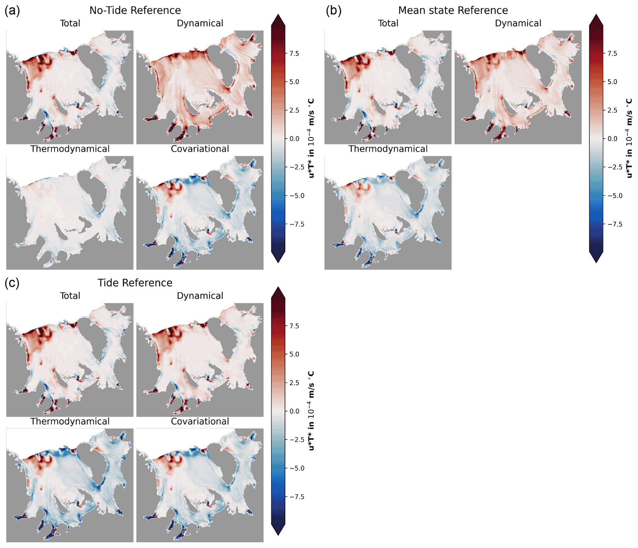
Figure C1 Dynamical–thermodynamical decomposition: the impact of the reference state. Contributions of thermodynamical, dynamical and covariational effects to tidal melting when choosing (a) the no-tide experiment, (b) the mean between no-tide and tide case, and (c) the tide experiment as reference. The mathematical descriptions for each case are shown in Eqs. (C1), (C2) and (C4), also explaining why the central case has no covariational contribution. For the tide reference case the negative of the total, dynamical and thermodynamical contributions have been plotted for better comparison. The contributions are sensitive to the choice of the reference.

Figure C1 shows the results of the decomposition analysis for all three approaches for the Filchner–Ronne Ice Shelf. The contributions of the individual components are qualitatively different, exhibiting progression in the thermodynamic and dynamic terms when going from the non-tidal to the central to the tidal reference state (or vice versa). We attribute this behaviour to approximation errors that occur when using linear methods to model a large perturbation (tides on/off) in a highly non-linear system (ocean–ice-shelf interaction). This study aims to understand the processes responsible for the difference between the two states, and, thus, we approximate using the mean. This choice has the advantages of being direction invariant (the removal of tides leads to the exact negative) and giving no covariational term, which simplifies the interpretation. However, the other cases might be more useful in other studies. For example, when developing a tidal-melt parameterization that is applied to non-tidal models (as done by Jourdain et al., 2019), the non-tidal case as the reference state might be the most straightforward approach. Similarly, to understand the effects of excluding tides from a model, choosing the tidal state as reference seems logical.

Appendix D: Tidal residual circulation

To estimate the residual circulation due to tide–topography interaction alone, we have performed a pseudo-barotropic simulation (similar to Mueller et al., 2012, 2018; Maraldi et al., 2013; Jourdain et al., 2019). For this experiment, heat and salt fluxes at the ice shelf base are set to zero, ocean surface fluxes are turned off, and we impose no velocities at the lateral boundaries other than from the tidal forcing. We use a constant density of 1027.83 kg m⁻³. Tidal forcing is applied as described in the main paper using sea surface height and barotropic currents (see Sect. 2.1). The ocean starts from a state of rest, and the spin-up period is 2 years. Figure D1 shows the depth-averaged annual mean circulation of the pseudo-barotropic experiment.

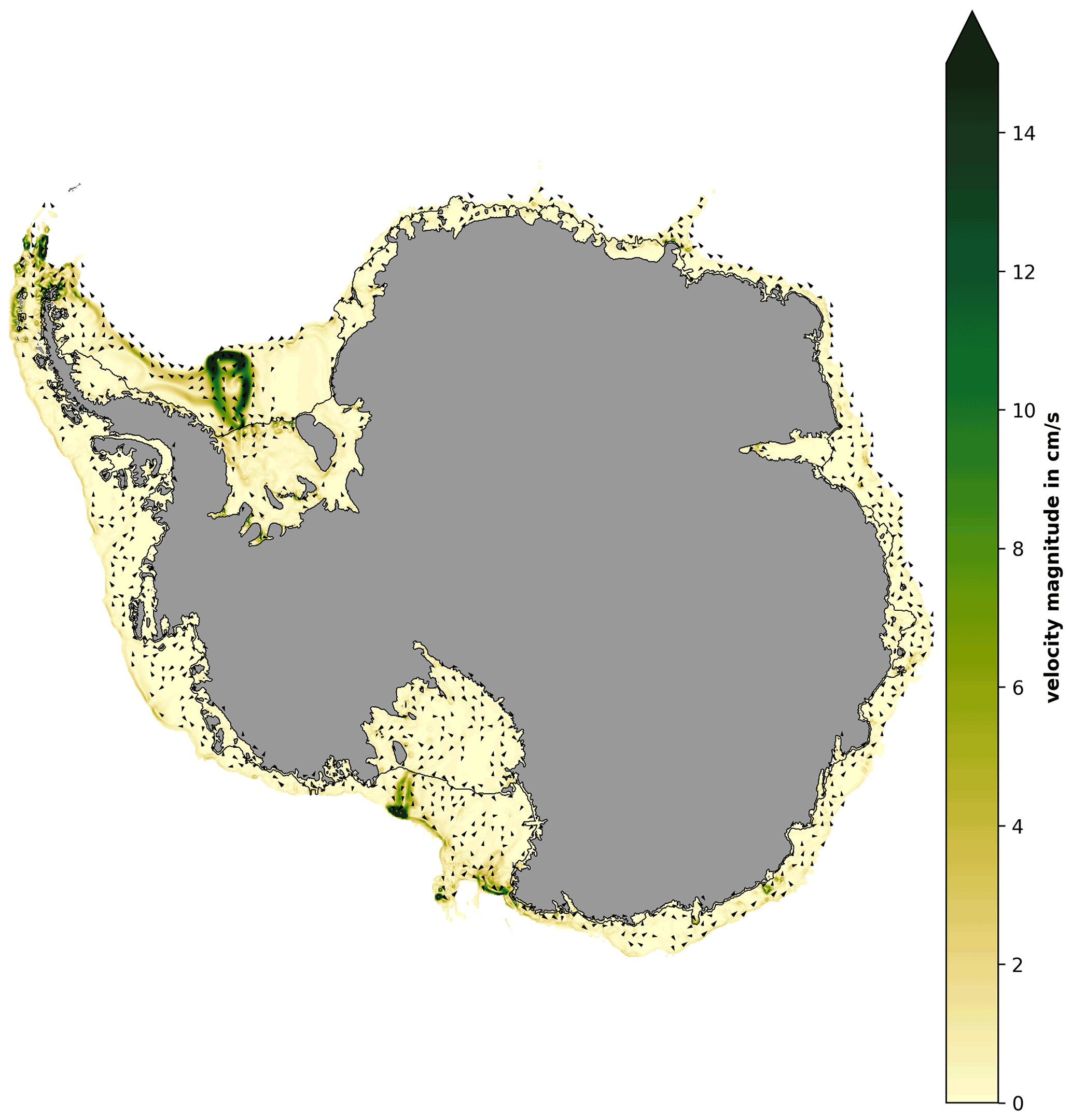
Figure D1 Tidal residual circulation from tide–topography interaction. Annual mean circulation of a tidal simulation without surface forcing, thermodynamic ice shelf interaction or stratification.