the Creative Commons Attribution 4.0 License.
the Creative Commons Attribution 4.0 License.
 | 11 Apr 2022
Net effect of ice-sheet–atmosphere interactions reduces simulated transient Miocene Antarctic ice-sheet variability
Constantijn J. Berends
Meike D. W. Scherrenberg
Roderik S. W. van de Wal
Edward G. W. Gasson
Benthic δ18O levels vary strongly during the warmer-than-modern early and mid-Miocene (23 to 14 Myr ago), suggesting a dynamic Antarctic ice sheet (AIS). So far, however, realistic simulations of the Miocene AIS have been limited to equilibrium states under different CO2 levels and orbital settings. Earlier transient simulations lacked ice-sheet–atmosphere interactions and used a present-day rather than Miocene Antarctic bedrock topography. Here, we quantify the effect of ice-sheet–atmosphere interactions, running the ice-sheet model IMAU-ICE using climate forcing from Miocene simulations by the general circulation model GENESIS. Utilising a recently developed matrix interpolation method enables us to interpolate the climate forcing based on CO2 levels (between 280 and 840 ppm), as well as varying ice-sheet configurations (between no ice and a large East Antarctic Ice Sheet). We furthermore implement recent reconstructions of Miocene Antarctic bedrock topography. We find that the positive albedo–temperature feedback, partly compensated for by a negative feedback between ice volume and precipitation, increases hysteresis in the relation between CO2 and ice volume. Together, these ice-sheet–atmosphere interactions decrease the amplitude of Miocene AIS variability in idealised transient simulations. Forced by quasi-orbital 40 kyr forcing CO2 cycles, the ice volume variability reduces by 21 % when ice-sheet–atmosphere interactions are included compared to when forcing variability is only based on CO2 changes. Thereby, these interactions also diminish the contribution of AIS variability to benthic δ18O fluctuations. Evolving bedrock topography during the early and mid-Miocene also reduces ice volume variability by 10 % under equal 40 kyr cycles of atmosphere and ocean forcing.
- Article
(5255 KB) - Full-text XML
-
Supplement
(1065 KB) - BibTeX
- EndNote


The dynamics of the Antarctic ice sheet (AIS) during the early and mid-Miocene (23 to 14 Myr ago) are a topical issue in palaeoclimate science. This issue is of great interest because over the course of this period the climatic conditions, such as the atmospheric CO2 concentration (Kürschner et al., 2008; Foster et al., 2012; Badger et al., 2013; Greenop et al., 2014; Super et al., 2018; Steinthorsdottir et al., 2021b), ranged from those of the recent past to those predicted for the future (∼ 200 to > 800 ppm; see Steinthorsdottir et al., 2021a, for a review). Benthic δ18O records show sizeable orbital-timescale fluctuations during this time, an indication of potential vigorous Antarctic ice volume variability (e.g. Zachos et al., 2008; Liebrand et al., 2011, 2017; Holbourn et al., 2013; Levy et al., 2019). The δ18O signal is, however, also shaped by deep-sea temperature changes. How much of the signal is committed by each component, and thus how the AIS evolved during the Miocene, is currently still under debate. On the one hand, geological evidence supports strong AIS dynamism (Pekar and DeConto, 2006; Shevenell et al., 2008), with ice periodically advancing and retreating, e.g. over Wilkes Land (Sangiorgi et al., 2018) and the Ross Sea sector (Hauptvogel and Passchier, 2012; Levy et al., 2016; Pérez et al., 2021). Some studies, on the other hand, advocate a more stable small AIS based on ice-proximal sea-surface temperature records from dinoflagellate cyst assemblages (Bijl et al., 2018) and TEX86 data (Hartman et al., 2018). In addition, a recent analysis of clumped isotope and records has found high bottom-water temperatures, which combined with the benthic δ18O record paradoxically suggest a Miocene AIS volume persistently larger than in the present day (Modestou et al., 2020). Finally, using climate modelling and data comparisons, it has been suggested that the AIS varied mostly in spatial extent, rather than volume, which imprinted on Miocene δ18O variability through a strong effect on deep-water temperatures (Bradshaw et al., 2021).
Ice-sheet models can be used to understand the physical processes driving Miocene AIS variability. Broadly stated, earlier modelling efforts have followed two approaches to this task. One approach is to use ice-sheet models bidirectionally coupled to climate models with as much physical realism in terms of processes included and resolution as is computationally feasible for long-term simulations. Gasson et al. (2016) adopted this approach, using an isotope-enabled set-up of a 3D ice-sheet model coupled to a regional climate model nested in a general circulation model (GCM). They showed the importance of including ice-sheet–climate feedbacks, ice-calving parameterisations, and changes in the ice sheet's oxygen isotopic composition for simulating strong AIS-induced benthic δ18O changes. Halberstadt et al. (2021) used the same model set-up to determine the influence of CO2 changes and uplift of the Transantarctic Mountains on glacial variability during the Miocene. These studies were so far limited to steady-state simulations, in which the climate forcing is kept constant until the ice sheet has equilibrated. Transient ice-sheet behaviour can be very different, as was, for example, demonstrated for the North American and Eurasian ice sheets during the Late Pleistocene (Abe-Ouchi et al., 2013). The second approach, which is the one taken in this study, is therefore to focus on transient AIS changes, applying gradually changing climatic conditions. Earlier studies employed 1D ice-sheet models in combination with parameterised temperatures (De Boer et al., 2010) or relatively simple climate models (Langebroek et al., 2009, 2010; Stap et al., 2017). Recently, Stap et al. (2019) showed that orbital-timescale CO2 changes cause smaller transient AIS variability than equilibrium simulations suggest by using the 3D thermodynamical Parallel Ice Sheet Model (PISM) forced by Miocene climates obtained from GCM (COSMOS) simulations (Stärz et al., 2017). Conceptual considerations indicate that the disequilibrium between ice volume and CO2 also leads to out-of-phase changes in these quantities (Stap et al., 2020). However, the COSMOS climate simulations were performed using only one ice-sheet configuration. Hence, the effect of surface whitening (darkening) by ice-sheet advance (retreat) on temperature, the so-called albedo–temperature feedback, was not included, nor was the ice-sheet desertification effect, i.e. the reduction of snow deposition on a growing ice sheet (e.g. Oerlemans, 2004). Furthermore, the effect of mass balance changes due to surface height changes (surface-height–mass-balance feedback) could only be crudely captured using a scalar lapse-rate correction for temperature, which is known to be a simplification (Fortuin and Oerlemans, 1990). Moreover, a present-day Antarctic bedrock topography was used, while during the Miocene the topography was different, which also significantly affects the surface mass balance and ice flow (Stap et al., 2016; Colleoni et al., 2018; Paxman et al., 2020).
In this study, we expand the scope of previous studies by performing transient simulations (cf. Gasson et al., 2016; Colleoni et al., 2018; Paxman et al., 2020; Halberstadt et al., 2021), now including ice-sheet–atmosphere interaction (cf. De Boer et al., 2010; Stap et al., 2016, 2017). We run the 3D thermodynamical ice-sheet model IMAU-ICE (De Boer et al., 2013; Berends et al., 2018), which is based on the commonly used shallow ice and shallow shelf approximations and is therefore comparable to PISM. Climate forcing is obtained from Miocene simulations by the GCM GENESIS, in which different CO2 levels and ice-sheet configurations ranging from zero ice to a substantial East Antarctic Ice Sheet are applied (Burls et al., 2021). Utilising a recently developed matrix interpolation routine (Berends et al., 2018), this set-up enables us to interpolate the climate forcing based on land ice changes in addition to CO2 changes. In this manner, the effects of ice-sheet changes on local temperatures and precipitation are represented. Because surface height changes are incorporated in the forcing, the surface-height–mass-balance feedback is captured more realistically as well. We perform both equilibrium simulations, keeping the forcing CO2 level constant, and idealised transient experiments, in which we vary the CO2 level on long and short quasi-orbital timescales (40, 100, and 400 kyr). We compare experiments using the matrix interpolation method to ones in which we use a simpler index method to obtain climate forcing variability only based on CO2 changes. In this way, we quantify the influence of the ice-sheet–atmosphere feedbacks on the variability in the AIS during the Miocene. In addition, we investigate the effect of bedrock topography changes over the Miocene by using topographies pertaining to the early (23–24 Myr ago) and mid-Miocene (14 Myr ago) (Hochmuth et al., 2020a; Paxman et al., 2019). We also carry out simulations using Eocene (34 Myr ago) and present-day bedrock topographies. Lastly, we test the sensitivity of our results to the parameterisation of basal melt underneath the floating ice shelves. This is achieved by performing identical simulations to our reference experiment but imposing relatively mild as well as harsh sub-shelf melt rates, easing and prohibiting ice shelf growth respectively. We quantify where and under which conditions ice shelves form and perish in our simulations, as well as how they influence the variability in the grounded ice volume.
For this study, we employ the ice-sheet model IMAU-ICE (v1.1.1-MIO) (De Boer et al., 2013; Berends et al., 2018) to simulate the Antarctic ice sheet using atmospheric input data obtained from Miocene climate simulations by the GCM GENESIS (Burls et al., 2021).
2.1 Ice-sheet model
IMAU-ICE is a 3D thermodynamical ice-sheet model, which uses a superposition of the shallow ice approximation (SIA) and shallow shelf approximation (SSA) to simulate the dynamics of grounded and floating ice. In the interior of the ice sheet, the ice flow is dominated by the SIA, while towards the fast-flowing ice streams on the fringes the SSA gains importance, becoming the governing component on the ice shelf (Winkelmann et al., 2011). No additional grounding-line parameterisations are included. We use a 40×40 km resolution grid covering the Antarctic continent. This resolution ensures the feasibility of performing a large number of simulations while still capturing the Antarctic ice flow in the amount of detail we deem appropriate for our purpose. Longitude and latitude coordinates are assigned to the grid using an inverse oblique stereographic projection (Reerink et al., 2010). For further settings, please see Appendix A.
2.1.1 Basal mass balance
Basal melt underneath the ice shelves (M(x,y)) is calculated using a combination of the parameterisation of Pollard and DeConto (2009) and a linear relation to ocean temperature change (Beckmann and Goosse, 2003; Martin et al., 2011):
with
Weighing factor zdeep grows with water depths (hw(x,y)) greater than 1800 m:
and zexpo(x,y) depends on the widest subtended angle to the open ocean (αsub(x,y)) and the shortest linear distance to the open ocean (ropen(x,y)):
Both factors are clipped at 0 and 1. The melt rate for the exposed shelves (Mexpo) varies linearly between 3 m yr−1 for an applied CO2 concentration of 280 ppm to 6 m yr−1 for CO2 concentrations of 400 ppm and higher. The melt rate for the deep-water shelves (Mdeep) similarly varies between 5 and 10 m yr−1. Melt rate Sm(x,y) is dependent on the water density (ρw), specific heat (cp), thermal exchange velocity (γT), water temperature (Twater), pressure-adjusted freezing point (Tfreeze(x,y)), latent heat of fusion (Hfus), and shelf ice density (ρi). Because GENESIS has a slab ocean component (Sect. 2.2), realistic water temperatures cannot be taken from the GCM results (Gasson et al., 2016; Halberstadt et al., 2021). Instead, we use an ad hoc global ocean temperature parameterisation adapted from De Boer et al. (2013). Similar to melt rates Mexpo and Mdeep, Tw varies linearly as a function of CO2 between −1.7 ∘C (280 ppm) and 2 ∘C (≥ 400 ppm).
Currently, calving is neglected. The only calving routine implemented in IMAU-ICE is thickness calving, i.e. calving floating ice with a thickness below a certain threshold. We exclude this in our simulations because it could hinder the growth of new ice shelves (e.g. Ritz et al., 2001). In combination with the heavily parameterised sub-shelf melt calculation, this makes the mass balance of the ice shelves arguably a weak point of our modelling effort. We therefore perform sensitivity experiments (Table 1) to investigate how our results depend on ocean forcing. We consider an extreme case using Last Glacial Maximum (LGM)-like melt parameter settings: Mexpo=0 m yr−1, Mdeep=2 m yr−1, and ∘C (De Boer et al., 2013). In another experiment, ice shelves are effectively inhibited from growing by applying a constant melt rate of 400 m yr−1 similar to the ABUM experiment of the ice-sheet model intercomparison project ABUMIP (Sun et al., 2020). By comparing the results of these extreme scenarios to our reference experiment, we can quantify where and under which conditions ice shelves form, as well as how they subsequently influence the variability in the grounded ice volume.
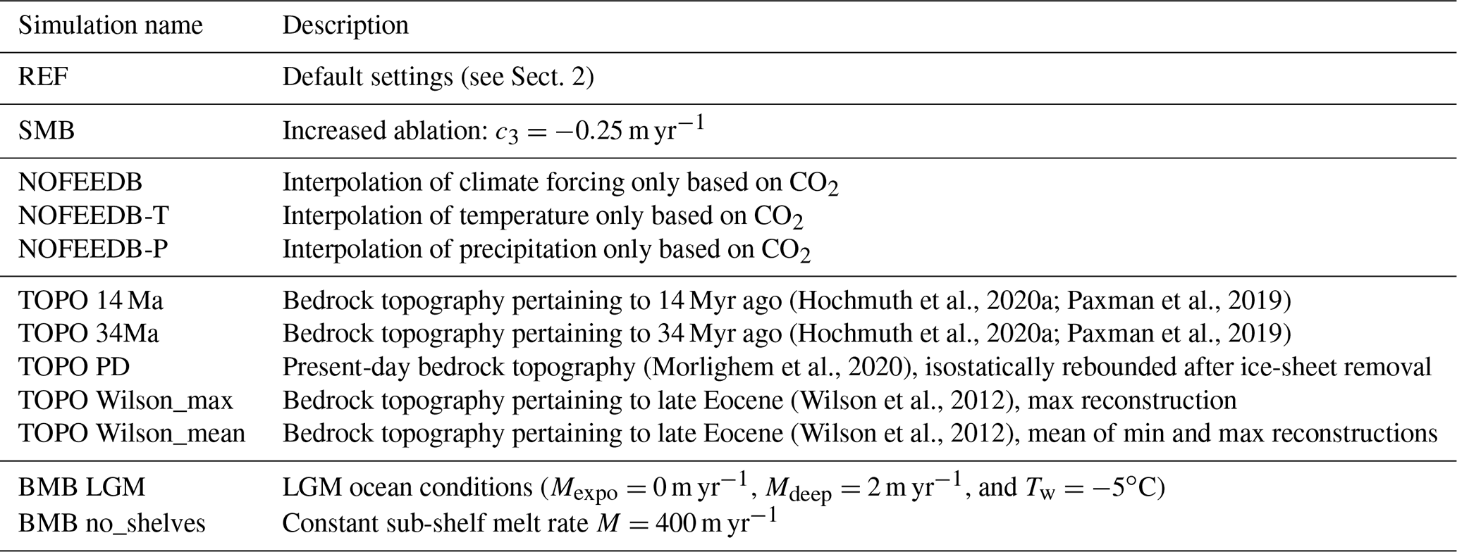
(Hochmuth et al., 2020a; Paxman et al., 2019)(Hochmuth et al., 2020a; Paxman et al., 2019)(Morlighem et al., 2020)(Wilson et al., 2012)(Wilson et al., 2012)Table 1Name and description of the experiments carried out. Each experiment comprises 15 simulations, as explained in the main text and listed in Table 2.
2.1.2 Surface mass balance
The surface mass balance (SMB) calculation uses precipitation (Papplied(x,y)) and 2 m air temperature (Tapplied(x,y)) obtained from Miocene climate simulations by GENESIS (Sect. 2.2) utilising a matrix interpolation routine (Sect. 2.3, Appendix B). The GENESIS fields are remapped from their native T31 grid (Sect. 2.2) to the ice-sheet model grid using bilinear interpolation based on longitude and latitude. Monthly SMB is the sum of accumulation and refreezing minus ablation (Berends et al., 2018). Refreezing is dependent on the available liquid water content, and the superimposed water content (Huybrechts and de Wolde, 1999; Janssens and Huybrechts, 2000). Accumulation (Acc(x,y)) is calculated as follows:
with fsnow(x,y) being the temperature-dependent snow fraction (Ohmura, 1999). Ablation (Abl(x,y)) follows from an insolation–temperature melt parameterisation (Bintanja et al., 2002):
The parameters are set to c1=0.788 m yr−1 K−1, c2=0.004 m3 J−1, and m yr−1. The internally calculated monthly albedo (α(x,y)) is derived as follows. First, a background albedo (αbg(x,y)) is determined: 0.1 for ocean-covered grid cells, 0.2 for soil, and 0.5 for ice. Thereafter, the effect of snow, with an albedo (αsnow) of 0.85, is added:
where Abl is the ablation calculated for the previous year. The firn layer depth (zfirn(x,y), clipped at 0 and 10 m) is changed over time by the addition of snowfall minus melt. The albedo α(x,y) is not allowed to be lower than the background albedo or higher than the albedo of snow. In Eq. (6), incoming solar radiation at the top of the atmosphere QTOA(x,y) is taken from Laskar et al. (2004) and kept constant at the present-day values so as to isolate climate variability caused by CO2 changes. This surface mass balance parameterisation has recently been shown to yield realistic results over the present-day Greenland ice sheet (Fettweis et al., 2020).
2.2 Climate model
GENESIS (version 3.0) (Thompson and Pollard, 1997; DeConto et al., 2012) has a spectral resolution of T31 (∼ 3.75∘ × 3.75∘). The atmospheric model is coupled to 2∘ × 2∘ surface models including a non-dynamical 50 m slab diffusive mixed-layer ocean with dynamic sea ice and dynamic vegetation. The applied palaeogeography comes from Herold et al. (2008), with dedicated modifications to Antarctica based on simulations by DeConto and Pollard (2003). Different simulations were carried out as described in Burls et al. (2021). Here, we use simulation 1fumebi for the cold climate and simulation 3nomebi for the warm climate (Fig. S1 in the Supplement). Simulation 1fumebi has a CO2 level of 280 ppm (1 × pre-industrial (PI)) and an AIS configuration with a full East Antarctic Ice Sheet (18.975×10⁶ km3 volume, area shown in Fig. S2). Simulation 3nomebi is forced by a CO2 level of 840 ppm (3 × PI) with no ice cover. Both simulations use present-day orbital settings. The vegetation on non-glaciated land, which has an influence on the regional climate, is determined by the dynamic vegetation model BIOME4.
2.3 Matrix interpolation method
The applied climate forcing is interpolated between the cold (1fumebi) and warm (3nomebi) GENESIS fields using a matrix interpolation method (Berends et al., 2018), described in detail in Appendix B. Briefly, the applied temperature interpolation is based on a prescribed value for CO2 and on the internally modelled ice sheets. The higher (lower) the CO2 level and the smaller (larger) the ice coverage, the more the climate forcing is like the warm (cold) climate. The feedback of the ice sheets on the climate is calculated via the effect on absorbed insolation through changes in surface albedo. The precipitation interpolation is determined solely from the ice volume. Because the cold climate is generally drier, this constitutes a negative ice-volume–precipitation feedback, representing the ice-sheet desertification effect in our simulations.
2.4 Simulations
We perform an experiment using our default settings (REF), as well as 11 sensitivity experiments with settings altered as indicated in Table 1. Each experiment consists of 15 simulations, 11 of which are steady state and 4 of which are transient simulations (Table 2).
Table 2Description of the 15 simulations spanning each experiment.
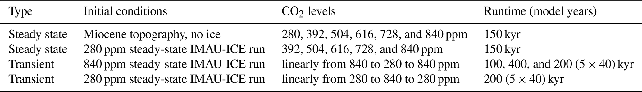
The steady-state simulations are run for 150 kyr with a constant forcing CO2 level – enough time for the ice sheet to equilibrate with the forcing climate. Mind that the CO2 level, rather than the climate itself, is kept fixed, which means the climate can still change due to land ice changes. First, six of these steady-state simulations are run using CO2 levels bracketing the 280 to 840 ppm range: 280, 392, 504, 616, 728, and 840 ppm. In our reference case, the initial conditions are obtained from recent reconstructions of the Antarctic bathymetry (Hochmuth et al., 2020a) and bedrock topography (Paxman et al., 2019) pertaining to 23 to 24 Myr ago (dataset: Hochmuth et al., 2020b). No ice is present at the start of these runs. These simulations constitute the lower, ascending branch of the hysteresis curve in the equilibrium CO2–ice-volume relation (blue connected diamonds in figures, e.g. Fig. 1b). Thereafter, the remaining five steady-state simulations are continued from results of the 280 ppm IMAU-ICE run, with CO2 levels of 392, 504, 616, 728, and 840 ppm. These simulations constitute the upper, descending branch of the hysteresis curve in the equilibrium CO2–ice-volume relation (red connected diamonds in figures, e.g. Fig. 1b).
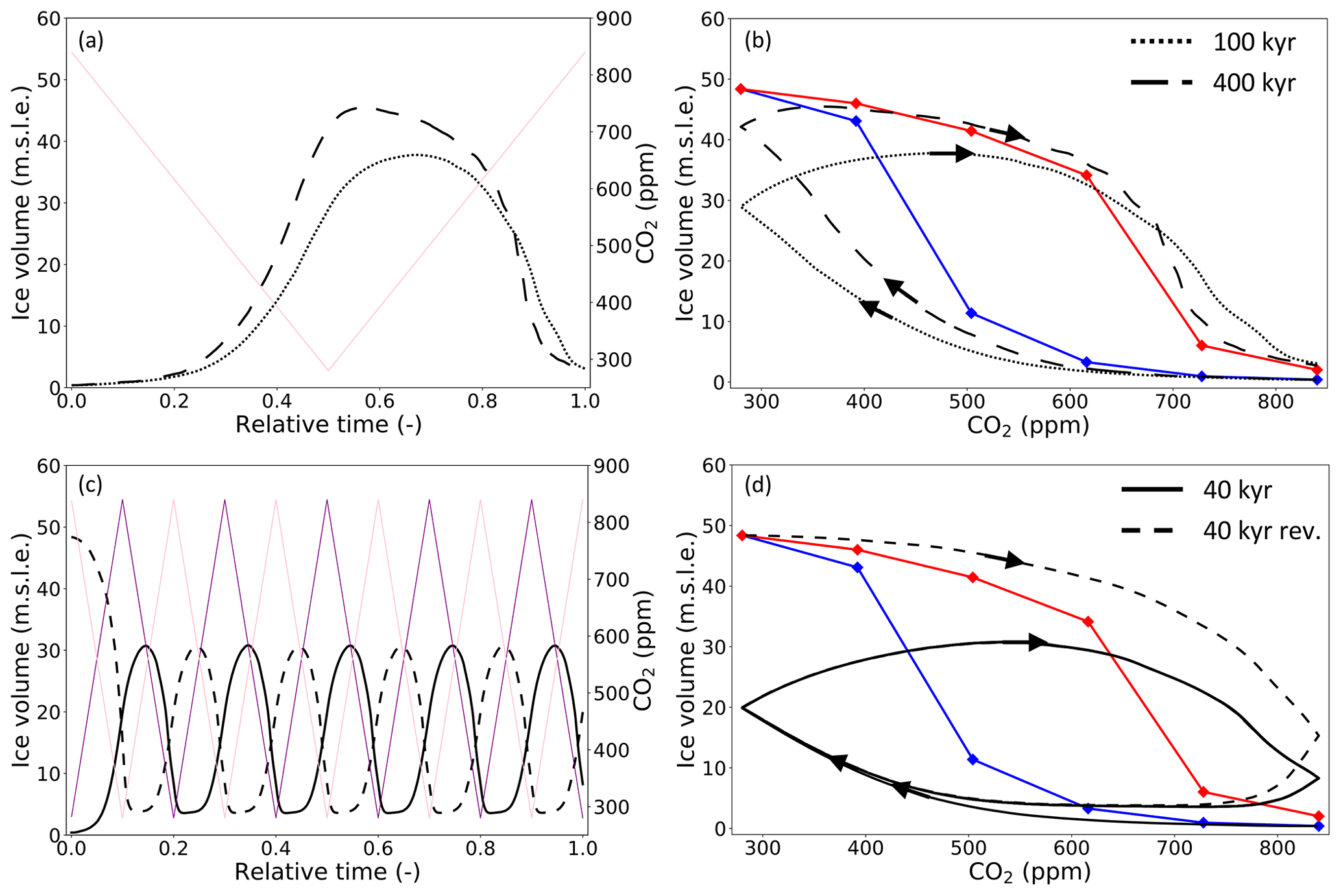
Figure 1(a) Evolution of forcing CO2 levels (pink) and ice volume above flotation (in metres sea level equivalent; black) over time (relative to the length of the simulation) for the transient 100 kyr (dotted) and 400 kyr (long-dashed) REF simulations. (b) Relation between CO2 and equilibrium ice volume (ascending branch, blue; descending branch, red) and transient ice volume (black as in a). (c, d) Same for the transient 40 kyr simulations starting from warm (CO2 pink, ice volume solid black) and cold (CO2 purple, ice volume dashed black) conditions. Arrows in (b) and (d) indicate the progression direction of ice volume. In (d), the transient ice volume evolutions of both simulations partly overlap.
Next, we perform the idealised transient simulations (Table 2). Three of these are started from the final state of the equilibrium 840 ppm IMAU-ICE run. The evolution of CO2 over time has a triangular shape (e.g. pink line in Fig. 1a). The CO2 is first linearly reduced from 840 to 280 ppm and then increased back to 840 ppm. In the three simulations, this triangular CO2 evolution is implemented over the course of 100 and 400 kyr and five consecutive times over 40 kyr (200 kyr in total; e.g. pink line in Fig. 1c). The final transient simulation is continued from the 280 ppm IMAU-ICE run and forced with an inverted triangular 40 kyr CO2 evolution. That means the CO2 is first linearly increased from 280 to 840 ppm and then decreased back to 280 ppm (e.g. purple line in Fig. 1c).
3.1 Reference simulations
As a minimal check for model performance and parameter settings, we first perform steady-state control simulations as in de Boer et al. (2015). These are executed using ERA40 present-day (PD; 1957–2002) precipitation and temperature forcing (Uppala et al., 2005). Constant present-day-like melt parameter settings are used to calculate the basal mass balance: Mexpo=3 m yr−1, Mdeep=5 m yr−1, and ∘C. Depending on whether the run is started from BedMachine PD ice and topography (Morlighem et al., 2020) or without ice and an isostatically rebounded topography, we simulate a total ice volume above flotation of 56.6 m sea level equivalent (m s.l.e.; 23.1×10¹⁵ m3) or 55.0 m s.l.e. (22.4×10¹⁵ m3) respectively. This is very close to the 55.0 m s.l.e. obtained from remapping the BedMachine data to our grid. Like other SIA- and SSA-based ice-sheet models (see de Boer et al., 2015), IMAU-ICE generally simulates slightly thinner ice in the interior and thicker ice along the margins (Fig. S3). The grounding line is simulated quite well, although it is slightly more advanced in the Filchner–Ronne and the Amery embayments. Due to lack of calving, the simulated ice shelves are extended much farther than the observations. However, since the increase in back pressure due to these overestimated shelf areas is very small (Reese et al., 2018b), this is unlikely to affect the evolution of the grounded ice. In this study, we will therefore focus on grounded ice.
In the reference equilibrium simulations using Miocene forcing (experiment REF), the AIS consists only of disconnected glaciers in high mountainous regions in the case of a 840 ppm CO2 level (Fig. 2a). It grows into a full East AIS (EAIS) and small West AIS (WAIS) in the case of 280 ppm forcing (Fig. 2b). In the latter case, the WAIS grounds on Marie Byrd Land and the peninsula, while it does not grow into the Ross and Filchner–Ronne embayments. Intermediate states for different forcing CO2 levels are shown in Fig. S4.
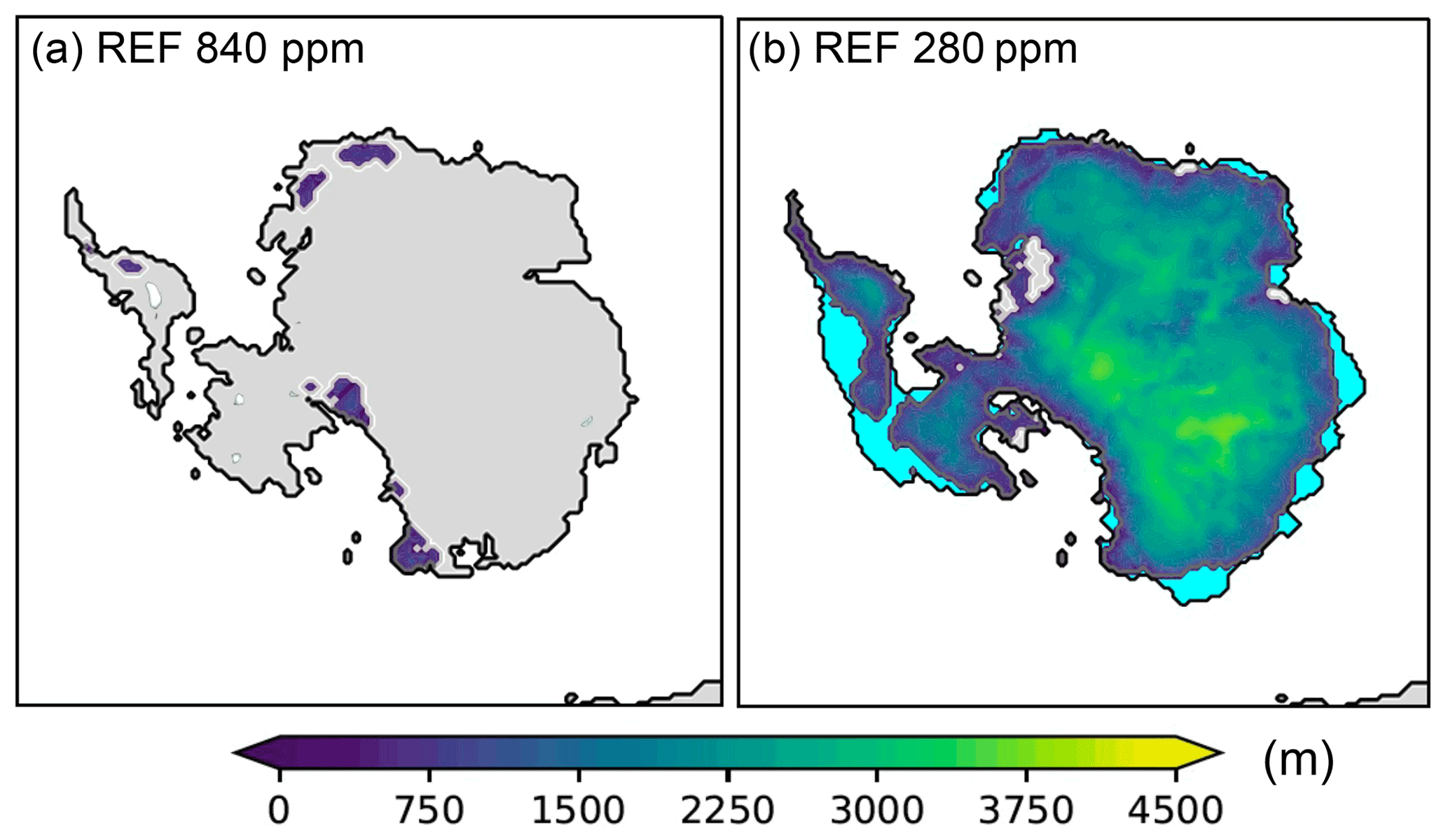
Figure 2 (a) Simulated equilibrated grounded ice thickness from experiment REF with 840 ppm and (b) 280 ppm CO2 forcing, starting without ice. Cyan areas indicate ice shelf extent and grey areas ice-free land.
We show the reference CO2 and equilibrium ice volume (above flotation) (Veq) relation in Fig. 1b (Pollard and DeConto, 2005). It decreases monotonically and exhibits considerable hysteresis, as displayed by the difference between the ascending (blue) and descending (red) branches. Transient simulations with different imposed timescales for the forcing variability are indicated by the dashed (400 kyr) and dotted (100 kyr) black lines. Peak ice volumes of 45.5 m s.l.e. (400 kyr) and 37.8 m s.l.e. (100 kyr) are yielded. In agreement with Stap et al. (2020), this peak is only reached later in time than the CO2 minimum (Fig. 1a). The peak is attained relatively earlier in time (Fig. 1a), i.e. at a lower CO2 level (Fig. 1b), in the 400 kyr simulation than in the shorter 100 kyr simulation. In the case of 40 kyr forcing cycles, the equilibrium cycle is attained very quickly and does not depend on the initial conditions (Fig. 1c, d; black lines partly overlapping). In the equilibrium cycle, the ice volume varies between 3.6 m s.l.e. at 728 ppm and 30.7 m s.l.e. at 532 ppm, a 27.1 m s.l.e. difference. Since the maximum ice volume is reached longer after the minimum CO2 level (252 ppm difference) than the minimum ice volume after the maximum CO2 level (112 ppm difference), the growth phase lasts longer than the decay phase. That also means that ice-sheet decay is on average 40 % faster than growth, but both rates, in particular the growth rate, are certainly not constant. In the transient simulations, the AIS initially builds up slowly in the high mountainous regions at ∼ 0.1 m s.l.e. kyr−1, speeding up to a maximum of 3 m s.l.e. kyr−1 when the surface mass balance (SMB) becomes positive on a large part of the continent as separate ice domes start to merge (gradients in Fig. 1c). When the transient ice volume is in between the ascending and descending branches of the equilibrium CO2–Veq relation, i.e. larger than the ascending (blue) volume but smaller than the descending (red) volume (Fig. 1d), the rate of transient ice volume change is relatively small (< 1 m s.l.e. kyr−1).
In earlier research using IMAU-ICE, different values for the SMB parameter c3 in Eq. (6) have been used (e.g. De Boer et al., 2013, 2014; Berends et al., 2018). Our reference setting C3=0.50 m yr−1 leads to satisfactory PD results, but using C3=0.25 m yr−1 as De Boer et al. (2014) did, a similar PD ice volume of 55.5 m s.l.e. is obtained (not shown). Using this setting (experiment SMB; Table 1) increases surface melt, with the onset of AIS growth and decay at lower CO2 levels (Fig. S5) as a result. Our REF settings yield an ice sheet similar in extent to the results of Stap et al. (2019) and DeConto and Pollard (2003) at 280 ppm, which disappears almost completely at 840 ppm. This ensures that we can most effectively study large-scale variability in the East Antarctic Ice Sheet. A different tuning would shift the CO2 at which these ice-sheet sizes are simulated but does not (qualitatively) affect the shape of the CO2–ice-volume relation.
3.2 Influence of ice-sheet–atmosphere interaction
Using a matrix interpolation routine enables us to interpolate the climate forcing for our ice-sheet model based on both CO2 and ice-sheet size. Here, we make a comparison to results of our model set-up using a simpler index routine, as, for example, used in Stap et al. (2019), in which the interpolation is solely based on the CO2 level. In experiment NOFEEDB (Table 1), we implement instead of Eqs. (B7) (for temperature) and (B11) (for precipitation) to interpolate between the cold (1fumebi) and warm (3nomebi) climates.
Because the positive albedo–temperature feedback is not invoked in this case, hysteresis in the CO2–Veq relation is smaller (Fig. 3b, solid and dashed red and blue lines). The temperature declines more quickly towards lower CO2 values, causing the equilibrium simulations to yield larger ice volumes (Fig. 3b, blue lines). At 280 ppm, Veq in the NOFEEDB case is 55.8 m s.l.e. compared to 48.4 m s.l.e. in the REF case. This difference in ice volume is mainly manifested in regions with low bedrock topography through a thicker WAIS in Marie Byrd Land, and EAIS in Mac. Robertson Land and Coats Land (not shown). Because the AIS deglaciates at similar levels as in the REF case (Fig. 3b, red lines), the difference between the CO2 levels of glaciation and deglaciation is smaller in the NOFEEDB case. That reduces the hysteresis in the CO2–Veq relation.
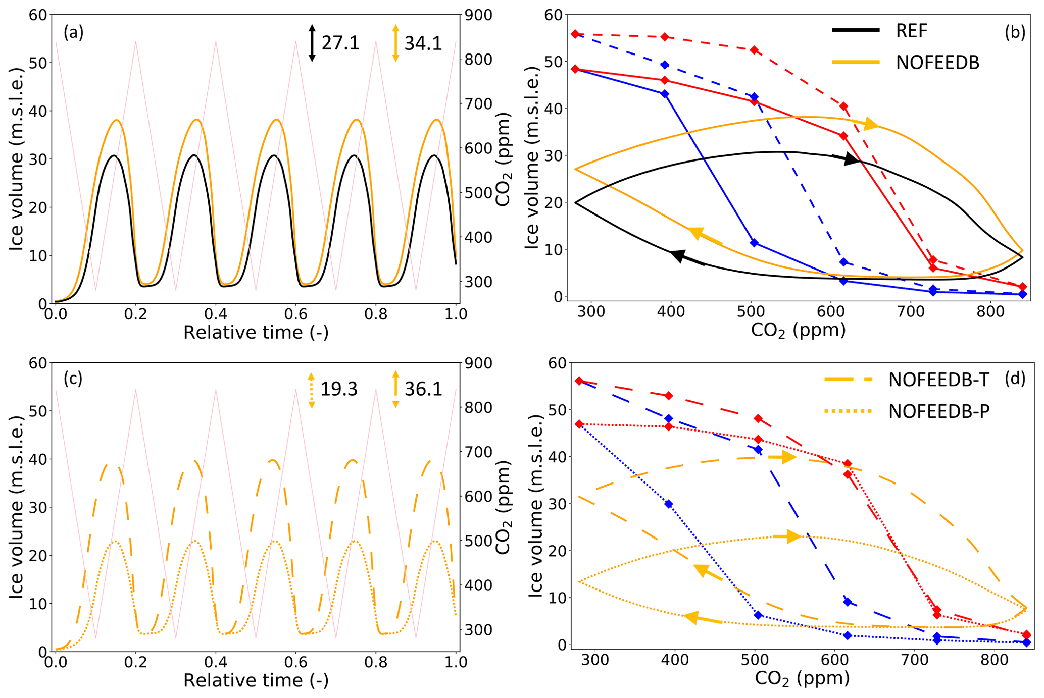
Figure 3(a) Evolution of forcing CO2 levels (pink) and ice volume over relative time for the transient 40 kyr REF (black) and NOFEEDB (orange) simulations. (b) Relation between CO2 and equilibrium ice volume (REF, solid red and blue; NOFEEDB, dashed red and blue) and transient ice volume (as in a). Only the equilibrium cycle (final 40 kyr) is shown. (c, d) Same for the NOFEEDB-P (dotted red, blue, and orange) and NOFEEDB-T (long-dashed red, blue, and orange) equilibrium and transient 40 kyr simulations. The amplitudes of transient ice volume variability (in m s.l.e.) in the equilibrium cycle are indicated in panels (a) and (c).
Transient ice volume variability is larger in the NOFEEDB case than in the REF case (Fig. 3a, b, black and orange lines). In the NOFEEDB case, peak ice volumes are increased to 54.3 m s.l.e. (400 kyr forcing CO2 cycle) and 47.4 m s.l.e. (100 kyr). Forced by 40 kyr CO2 cycles, the amplitude of variability is 34.1 m s.l.e. in the equilibrium cycle. That means the ice-sheet–atmosphere interactions that are included in the REF case decrease the amplitude of AIS variability by 21 %.
As mentioned above, the difference between the REF and NOFEEDB results is mainly governed by the albedo–temperature feedback. However, in the REF case, precipitation decreases with increasing ice volume, via Eq. (B10) combined with a cold climate that is generally drier. This constitutes a negative ice-volume–precipitation feedback. The effect of this feedback alone is shown by a comparison between the results of experiment NOFEEDB and those of NOFEEDB-P (Table S1, Fig. 3c, d). In the latter experiment, the index method is only used for precipitation, and temperature is interpolated in the normal sense (Eq. B7). The hysteresis in the CO2–Veq relation is now larger, and the amplitude of transient variability in the equilibrium cycle of the 40 kyr simulation is 19.3 m s.l.e., 43 % smaller than in the NOFEEDB case. In contrast, using the index method only for temperature (experiment NOFEEDB-T), the amplitude of 40 kyr transient variability becomes 6 % larger (36.1 m s.l.e.) than in the regular NOFEEDB case. The results of experiment NOFEEDB-T are much closer to those of experiment NOFEEDB. Therefore, of the two ice-sheet–atmosphere feedbacks, the albedo–temperature feedback is dominant in our experiments.
3.3 Effect of bedrock topography changes
Recent geological reconstructions have indicated that Antarctic bedrock topography has evolved substantially since the Eocene–Oligocene boundary (34 Myr ago) mostly due to thermal subsidence and glacial erosion (Paxman et al., 2019). In the REF simulations, we have used the bedrock topography reconstruction pertaining to the Oligocene–Miocene boundary (23–24 Myr ago). In experiment TOPO 14 Ma (Table 1), we instead use the one pertaining to the mid-Miocene (14 Myr ago). A larger part of West Antarctica (Marie Byrd Land and Palmer Land) has subsided below sea level in this reconstruction (Fig. S6a, b). This leads to a smaller simulated WAIS at low CO2 levels in the TOPO 14 Ma case (Fig. 4). The bedrock subsidence in Victoria Land and the Amery embayment has a smaller effect on equilibrium ice volume. The total equilibrium ice volume above flotation is 44.6 m s.l.e. at 280 ppm compared to 48.4 m s.l.e. in the REF case (−8 %). The amplitude of transient ice volume variability is affected as well, even on relatively short orbital (obliquity) timescales. It decreases to 24.4 m s.l.e (−10 % with respect to REF) when 40 kyr forcing cycles are imposed (Fig. 5).
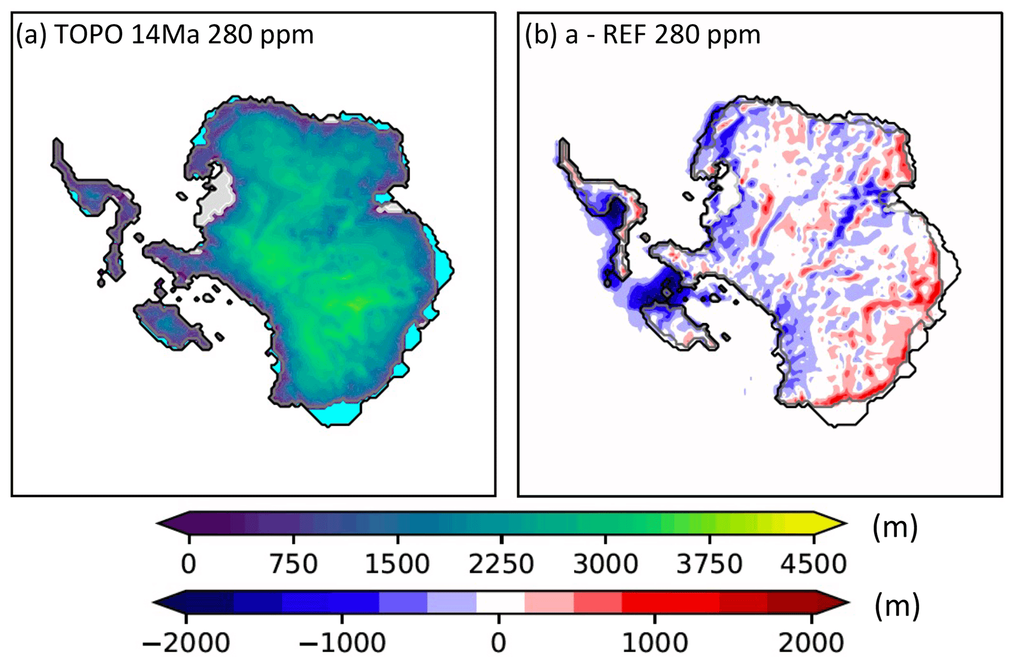
Figure 4(a) Simulated equilibrated grounded ice thickness from experiment TOPO 14 Ma with 280 ppm CO2 forcing. Cyan areas indicate ice shelf extent and grey areas ice-free land. (b) Difference in ice thickness between TOPO 14 Ma and REF with 280 ppm CO2 forcing (grounding line and continental edge as in a).
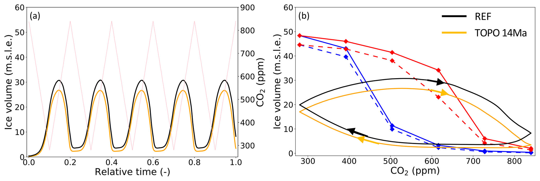
Figure 5(a) Evolution of forcing CO2 levels (pink) and ice volume over relative time for the transient 40 kyr REF (black) and TOPO 14 Ma (orange) simulations. (b) Relation between CO2 and equilibrium ice volume (REF, solid red and blue; TOPO 14 Ma, dashed red and blue) and transient ice volume (as in a). Only the equilibrium cycle (final 40 kyr) is shown.
The effect of long-term Antarctic landscape evolution on ice volume becomes more apparent when we compare simulations using bedrock conditions of the Eocene–Oligocene boundary (34 Myr ago; TOPO 34 Ma) and relaxed PD topography (TOPO PD) (Fig. S6c, d). In the latter case, less ice builds up in Victoria Land and Coats Land where the initial bedrock topography has subsided below sea level compared to the TOPO 14 Ma case (Fig. S7a). The equilibrium ice volume at 280 ppm reduces to 42.8 m s.l.e. (−12 % with respect to REF) and the amplitude of transient 40 kyr ice volume variability to 23.3 m s.l.e. (−14 % with respect to REF; Fig. S8a, b dotted lines). Conversely, it increases to 28.4 m s.l.e. (+5 % with respect to REF; Fig. S7b) and is centred around a generally larger ice volume in experiment TOPO 34 Ma (Fig. S8a, b, long-dashed lines). This is also due to the fact that the EAIS is more stable, as shown by larger ice volumes already at high CO2 levels in the CO2–Veq relation, particularly in the upper, descending branch. Hysteresis is indeed larger than in the REF case because the positive surface-height–mass-balance feedback is stronger due to the build-up of thicker ice. At 280 ppm, the equilibrium ice volume is 57.4 m s.l.e. in this experiment (+19 % with respect to REF). A much thicker ice sheet is built up in Coats Land, the Amery embayment, and Marie Byrd Land (Fig. S7b). Still in this case, the ice sheet does not significantly advance into the Ross and Filchner–Ronne embayments. This is different when we use the earlier geological reconstructions of Antarctic palaeotopography at the Eocene–Oligocene boundary of Wilson et al. (2012) (Fig. S6e, f). At 280 ppm, the ice then grounds in the Ross embayment (TOPO Wilson_mean, using the mean of the minimum and maximum reconstructions; Fig. S7c) or in both embayments (TOPO Wilson_max, using the maximum reconstruction; Fig. S7d). Due to the higher CO2 levels at which deglaciation takes place, a relatively large ice volume persists throughout 40 kyr transient simulations (Fig. S8c, d). In contrast to the other experiments, the initial conditions of these transient simulations now affect the ice volume during the equilibrium cycle. The ice sheet remains generally larger when the equilibrium 280 ppm simulation, rather than the 840 ppm simulation, is used as starting point (not shown).
3.4 Sensitivity to ocean forcing
We perform and compare two additional sensitivity experiments that are end-members with respect to basal melt rate settings to access the sensitivity of our results to the parameterisation of ocean forcing. In experiment BMB LGM (Table 1), we use Last Glacial Maximum (LGM)-like basal melt parameter settings in Eq. (1): Mexpo=0 m yr−1, Mdeep=2 m yr−1, and ∘C (De Boer et al., 2013). The mild basal melt rates in this case create an environment in which ice shelves can grow relatively easily. At the other extreme, in experiment BMB no_shelves, ice shelves are effectively inhibited from growing by applying a constant melt rate of 400 m yr−1. The effect of ice shelf formation becomes notable from 504 ppm in the equilibrium simulations (Fig. 6b, solid and dashed blue lines). Ice shelves form along the margins at Coats Land and Oates Land (Fig. 7a). While in Coats Land this leads to a modest thickening of the grounded ice, this happens to a much lesser degree in Oates Land. In the long 400 kyr transient simulation, these ice shelves form after around 110 kyr at ∼ 530 ppm (Fig. 6b). At 392 ppm in the equilibrium simulations, and after around 170 kyr at ∼ 360 ppm in the 400 kyr transient simulation, ice shelves appear approximately simultaneously along almost the entire remainder of the (east and west) Antarctic margin (Fig. 7b). The effect on grounded ice is particularly noticeable in West Antarctica, as well as Wilkes Land, George V Land, and Mac. Robertson Land, where the ice sheet thickens by kilometres. In the deglaciation phase these ice shelves remain influential until 728 ppm in the equilibrium simulations (Fig. 6b, solid and dashed blue lines) and until around 360 kyr at ∼ 728 ppm in the 400 kyr transient simulation (Fig. 6a, b, green and orange lines). In the transient simulations, the amplitude of variability is increased. The hysteresis in the CO2–V relation is increased as well, although only slightly. In the 40 kyr transient simulations, the ice volume variability amounts to 30.7 m s.l.e. in case LGM BMB and 25.7 m s.l.e. in case LGM no_shelves, a 5 m s.l.e. (19 %) difference (Fig. 6c, d).

Figure 6(a) Evolution of forcing CO2 levels (pink) and ice volume over relative time for the transient 400 kyr BMB no_shelves (solid orange) and BMB LGM (dashed green) simulations. (b) Relation between CO2 and equilibrium ice volume (BMB no_shelves, solid red and blue; BMB LGM, dashed red and blue) and transient ice volume. (c, d) Same for the transient 40 kyr simulations. Only the equilibrium cycle (final 40 kyr) is shown.
The CO2 levels at which East Antarctic glaciation is simulated are known to be dependent on the climate model used to construct the climate forcing (Gasson et al., 2014). This could (partly) explain why in our study EAIS inception occurs at higher CO2 levels than in Stap et al. (2019). They used climate forcing from COSMOS which has a higher climate sensitivity (reported as 4.1 K per CO2 doubling) than GENESIS (2.9 K). Note that in neither study are greenhouse gases other than CO2 varied, probably biassing the CO2 concentrations high. Another factor that has a large influence on the glaciation threshold is the ablation factor that we use in our surface mass balance calculation (C3 in Eq. 6), as demonstrated by our SMB sensitivity experiment (Fig. S5). Arguably the best way to further constrain this parameter in the future is by performing a comprehensive comparison of our mass balance calculation, and other methods and observations, as was done previously for the Greenland ice sheet (Fettweis et al., 2020). Differences in ice dynamics, e.g. in the treatment of ice flow enhancement and basal sliding, might cause further disparity. Probably for the same reasons, we obtain larger transient AIS volume variability than Stap et al. (2019) when using a similar index method (experiment NOFEEDB). We nonetheless corroborate that disequilibrium between the AIS and the forcing climate causes smaller transient ice volume variability than steady-state simulations suggest (Stap et al., 2019), as well as out-of-phase changes between these quantities (Stap et al., 2020).
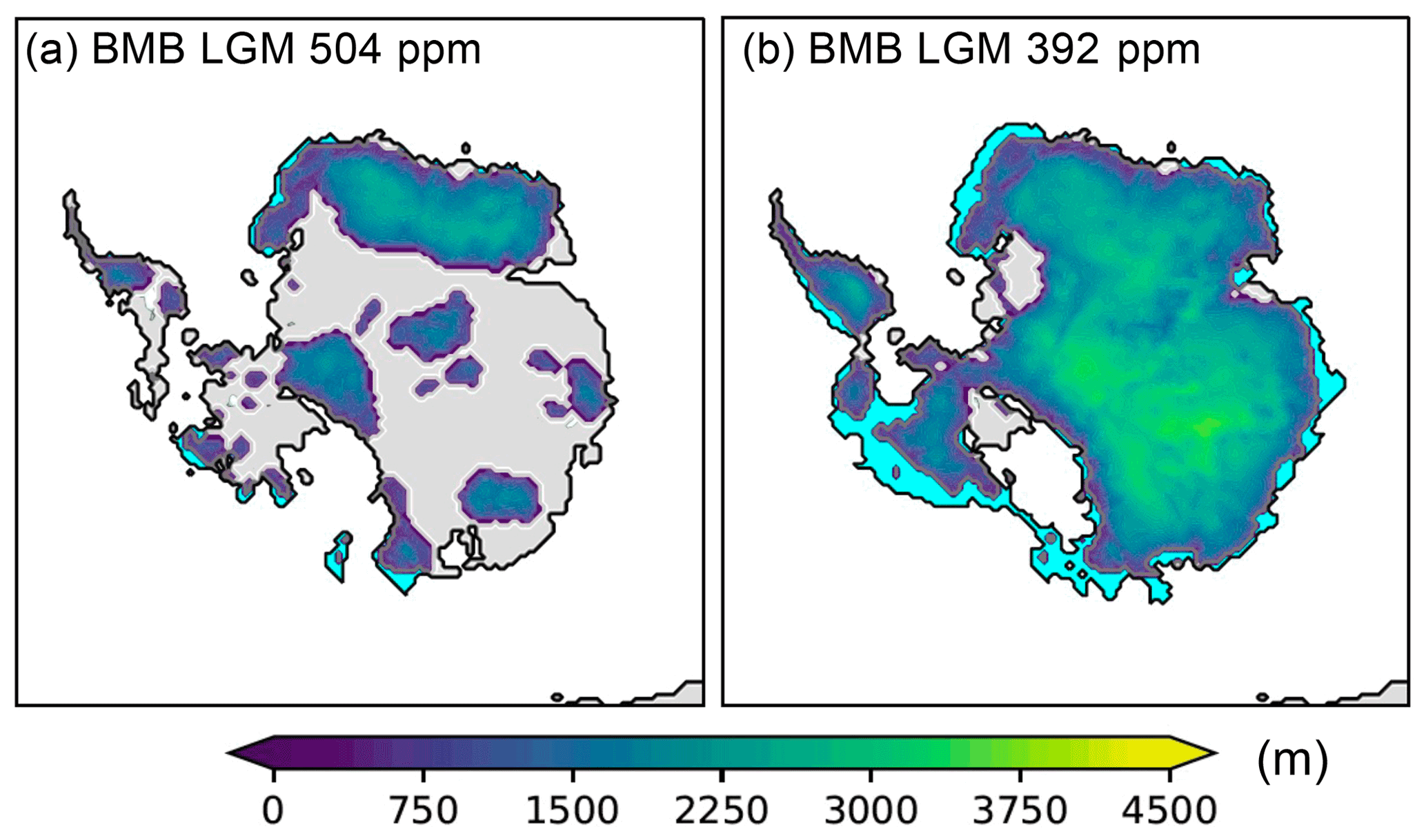
Figure 7(a) Simulated equilibrated grounded ice thickness from experiment BMB LGM with 504 ppm and (b) 392 ppm CO2 forcing, starting without ice. Cyan areas indicate ice shelf extent and grey areas ice-free land.
Here, we include ice-sheet–atmosphere feedbacks in our reference case. We have shown that these feedbacks tend to increase hysteresis in the CO2 and equilibrium ice volume relation and decrease the amplitude of AIS variability under equal 40 kyr forcing CO2 cycles by 21 % (Fig. 3). Also on longer timescales AIS variability is suppressed by the ice-sheet–atmosphere feedbacks. This is partly due to the smaller equilibrium ice volumes at low CO2 levels and partly to decreased growth rates of the transient ice volume relative to the change in equilibrium ice volume. In short, the ice-sheet–atmosphere feedbacks cause a slower build-up of the AIS to smaller peak ice volumes. Correspondingly, the contribution of AIS volume changes to benthic δ18O fluctuations gets smaller. This calls for a larger contribution of deep-sea temperatures to the amplitude of Miocene benthic δ18O fluctuations. The actual strength of the impact will, however, depend on the isotopic composition of Antarctic snow as well (Gasson et al., 2016; Rohling et al., 2021).
Furthermore, we use recent reconstructions of Antarctic bedrock topography during the Miocene (Hochmuth et al., 2020a; Paxman et al., 2019), rather than the present day as in Stap et al. (2019), as a boundary condition in our AIS simulations. In agreement with Colleoni et al. (2018) and Paxman et al. (2020), we find that the WAIS becomes more vulnerable over the early and mid-Miocene (Fig. 5). This is demonstrated by the lower equilibrium ice volumes at equal CO2 levels in our experiment TOPO 14 Ma, which has a bedrock topography pertaining to the mid-Miocene (14 Myr ago) compared to REF, in which the topography is from the Oligocene–Miocene boundary (23–24 Myr ago). We also corroborate the finding of Paxman et al. (2020) that from 34 to 24 Myr ago bedrock changes primarily concern the EAIS, while from 24 Myr ago onwards mostly the WAIS is affected. Here, we have additionally examined the effect of the evolving Antarctic landscape on transient Miocene AIS variability, which is 10 % smaller when subjected to 40 kyr forcing CO2 cycles in TOPO 14 Ma than in REF due to impeded WAIS growth. Hence, CO2 minima must have dropped increasingly further over the course of the early and mid-Miocene to obtain AIS variability with similar amplitude and consequently a similar contribution of the AIS to Miocene benthic δ18O variability.
In this study, we focus on the variability in a generally small AIS, which is located primarily on the east side of the continent, while the WAIS size remains relatively limited. In the Ross and Filchner–Ronne embayments growth of extended ice shelves never occurs in our Miocene simulations, not even when the basal melt rates are set to LGM values. On the one hand, it is certainly possible that our basal melt parameterisation is not suited for the simulation of (large-scale) Antarctic ice shelf inception. On the other hand, the fact that the Ross and Filchner–Ronne ice shelves do grow when we impose steady present-day climate forcing points out that West Antarctic ice shelves have to be sustained by a sufficiently large ice flow coming from the WAIS. That means that in addition to the oceanic conditions, suitable atmospheric conditions are very important for ice shelf formation as well. Therefore, WAIS growth is hampered by the air temperatures remaining too warm in our forcing climate simulations because in the cold case (simulation 1fumebi) there is only a small WAIS present (Fig. S2) in the forcing climate simulation. In the future, the forcing steady-state climate simulations used in the matrix interpolation should preferably be constructed by a coupled set-up of the same ice-sheet and climate models that are deployed in the transient simulations. This would ensure congruence between the results of the equilibrium and transient simulations so that the transient ice sheet will not grow beyond its largest size in the forcing equilibrium results.
Although the AIS remains mostly grounded, the formation of floating ice shelves does have an impact on our result. This is demonstrated by comparing simulations in which LGM basal melt rates are applied to simulations in which ice shelf growth is prevented (Figs. 6, 7). The 40 kyr transient AIS variability is amplified by 19 % in the case of LGM basal melt rates – and 5 % in the reference case – compared to the case without ice shelves. In our simulations, ice shelves first appear along the coasts of Oates Land and Coats Land when the CO2 concentration drops below ∼ 530 ppm (Tw=2 ∘C), but the effect of ice shelves on grounded ice volume only becomes significant below ∼ 360 ppm CO2 (Tw=0.8 ∘C) when the EAIS – with a volume of almost 30 m s.l.e. – is already well-established. This transition, from a land-based ice sheet to one that is in contact with the ocean, at CO2 levels around 400 ppm is in general agreement with other model results (Halberstadt et al., 2021) and geological data inferences (Naish et al., 2009; Levy et al., 2016, 2019). Below ∼ 360 ppm CO2, ice shelves fringe almost the entire continent in our simulations. This includes the Wilkes Subglacial Basin and the Ross Sea sector, where records from IODP (Integrated Ocean Drilling Program) site U1356 and ANDRILL AND-2A show evidence of periodic ice retreat and readvance (Hauptvogel and Passchier, 2012; Levy et al., 2016; Pérez et al., 2021; Sangiorgi et al., 2018). When we increase CO2 levels from cold conditions in our simulations, the ice shelves keep having an effect on grounded AIS ice volume until relatively high CO2 levels of ∼728 ppm (Tw=2 ∘C) are reached. Only then does the AIS retreat into the Wilkes Subglacial Basin, suggesting that in our model set-up periodic AIS waxing and waning in this region have to be governed by substantial CO2 fluctuations. Growth of ice shelves hence increases hysteresis in the CO2–ice-volume relation, in general agreement with the findings of Garbe et al. (2020). In line with this result, we find a different effect on final ice volume (above flotation) in steady-state PD simulations with a 400 m yr−1 melt rate depending on whether the simulation is started with or without ice. Starting from an isostatically rebounded PD topography without ice, we obtain a volume of 39.5 m s.l.e., 28 % smaller than the PD run with normal basal melt rates (Fig. S9a, c). When the simulation is started from a PD topography including grounded and floating ice, the final volume is 48.4 m s.l.e., which is only 14 % smaller than the normal PD run (Fig. S9b, d). Hence, in our model, the effect of ice shelves on grounded ice volume is smaller when existing ice shelves are melted away than when ice shelves cannot form in the first place. Despite having a longer model runtime and different surface mass balance forcing, these simulations are similar to the ABUMIP ABUM experiment (Sun et al., 2020). Our simulated 8.2 m s.l.e. loss of ice volume above flotation after ice-sheet removal under PD forcing conditions (starting with ice) is on the large side of the wide range of model responses (∼ 1 to 11 m s.l.e. loss) reported there. Showing complete collapse of the WAIS and strong retreat in the Amery embayment but limited ice loss in the Recovery, Wilkes, and Aurora subglacial basins, our spatial response is most similar to that of ABUMIP models PISM1, PSU3D1, and BISICLES. However, our simulated response, using a Coulomb sliding law (q=0.3), is weaker than that of Elmer/Ice and SICOPOLIS (Simulation Code for Polythermal Ice Sheets) which used a Weertman sliding law (m=3) and that of a different version of IMAU-ICE that used the Schoof flux boundary condition (Schoof, 2007) at the grounding line. A stronger response of grounded ice volume to ocean warming and ice shelf break-up might lead to earlier retreat, i.e. at a lower CO2 level, of the AIS in, for example, the Wilkes Subglacial Basin, hence reducing hysteresis in the CO2–ice-volume relation.
Our climate input comes from the same model (GENESIS) as Halberstadt et al. (2021), who obtain relatively large EAIS volumes at CO2 levels up to 1140 ppm. Differences between their results and ours can be explained by the different ice-sheet models and surface mass balance schemes used. We use an insolation temperature melt (ITM) scheme (Bintanja et al., 2002), accounting for the direct effect of insolation on surface melt, whereas they deploy a positive degree day (PDD) scheme. Additionally, they use a regional climate model for downscaling the forcing, which allows for capturing orographic precipitation in more detail. We use a bias correction to obtain a more detailed reference climate. This may, however, lead to overestimated temperatures because we use a present-day (ERA-40) base climate, which is slightly warmer than our PI reference (Stap et al., 2019). In model tests, we simulate higher AIS ice volumes at high CO2 levels when we refrain from using this bias correction, although this is dependent on the ablation factor (c3 in Eq. 6; not shown). All in all, even with the bias correction included, we need very large CO2 variations on relatively short orbital timescales (40 kyr) to obtain substantial East Antarctic Ice Sheet variability. This could point to a relatively stable EAIS and a consequent reduced contribution to benthic δ18O fluctuations during the Miocene (Bijl et al., 2018; Hartman et al., 2018). Alternatively, the WAIS could play a more major role in establishing ice-sheet variability. As explained above, WAIS growth is hampered in our simulations by the climate forcing. However, geological evidence was recently found for a dynamic Miocene WAIS in the Ross Sea section (Marschalek et al., 2021), in agreement with the modelling results of, for example, Gasson et al. (2016) and Halberstadt et al. (2021). The generally low benthic δ18O values during the Miocene in that case would require persistent high ocean temperatures, which were indeed recently found by Modestou et al. (2020). Further modelling efforts are still needed to reconcile these warm ocean temperatures with the existence of a large marine AIS.
Using the ice-sheet model IMAU-ICE, we have performed steady-state and transient simulations of the Antarctic ice sheet (AIS) during the early and mid-Miocene (23 to 14 Myr ago). Climate forcing was obtained from Miocene simulations by GENESIS (Burls et al., 2021), with different CO2 levels and ice-sheet configurations, using a recently developed matrix interpolation routine (Berends et al., 2018).
Compared to a simpler index method, as used, for example, in Stap et al. (2019), our matrix interpolation method incorporates two important ice-sheet–atmosphere feedbacks: the positive albedo–temperature feedback and a negative ice-volume–precipitation feedback. The former tends to increase hysteresis in the CO2 and ice volume above flotation (V) relation and decrease the amplitude of transient AIS variability. The negative ice-volume–precipitation feedback, which represents the ice-sheet desertification effect, has the opposite effect (Fig. 3). The albedo–temperature feedback is dominant in our simulations. In the 40 kyr transient reference simulation, the ice volume variability amplitude is 21 % smaller than when an index method is used. Hence, the net effect of accounting for ice-sheet–atmosphere interactions in the interpolation of climate forcing reduces simulated transient Miocene Antarctic ice-sheet variability.
Differences between the geological reconstructions of Antarctic bedrock topography at the Oligocene–Miocene boundary (23–24 Myr ago) and the mid-Miocene (14 Myr ago) are mainly located in West Antarctica. The subsidence of land below sea level during the early and mid-Miocene impedes WAIS build-up. Consequently, it diminishes hysteresis in the CO2–V relation and reduces 40 kyr AIS variability by 10 % in amplitude (Figs. 4, 5). Hence, CO2 minima must have dropped increasingly further over the course of the early and mid-Miocene to obtain AIS variability with similar amplitude.
Here, we have conducted idealised transient simulations, addressing the effect of CO2 variability on Miocene AIS evolution. Moving forward towards realistic transient simulations of AIS evolution, orbital forcing variability will need to be accounted for in the model set-up, for instance by integrating it in the matrix interpolation method (e.g. Ladant et al., 2014; Tan et al., 2018). A further improvement to be made is the implementation of a more advanced scheme to calculate the basal mass balance underneath the ice shelves; several alternatives have been developed in recent years (e.g. Reese et al., 2018a; Lazeroms et al., 2019; Pelle et al., 2019). This should be accompanied by ocean forcing supplied by sophisticated (3D) ocean models. As a final prospect, inclusion of a coupled sediment model will ultimately open up the possibility of quantifying the transient effect of changing bedrock topography on AIS dynamics over the Miocene (Pollard and DeConto, 2003, 2020).
In IMAU-ICE, Glen's flow law exponent is set to n=3, and the SIA- and SSA-based velocities are enhanced by factors of 5 and 1 respectively. The basal stress is calculated using a Coulomb power law model for pseudo-plastic till (exponent q=0.3 and threshold velocity uthreshold=100 m s−1) (Bueler and Brown, 2009). The till friction angle, which determines the yield stress, varies linearly between 5∘ for bedrock elevations of −1000 m and lower and 20∘ for those of 0 m and above. The geothermal heat flux is taken from Shapiro and Ritzwoller (2004). A basic elastic lithosphere-relaxing asthenosphere (ELRA) model (Lingle and Clark, 1985; Le Meur and Huybrechts, 1996) is used to calculate bedrock adjustment, using a mantle density of 3300 kg m−3, a lithospheric flexural rigidity of 1.0×1025 kg m2 s−2, and a relaxation time of 3000 years. The sea level is kept constant at present-day level (0 m) because local Antarctic sea level changes are very uncertain during the Miocene as they are mainly due to Antarctic ice-sheet changes. Local sea level changes can differ substantially from the global mean (e.g. Stocchi et al., 2013), and their calculation would require solving the sea level equation which is not yet available in IMAU-ICE. We have performed three tests applying a constant 7 m higher sea level (mimicking the absence of the Greenland ice sheet), as well as applying internally calculated global mean and minus the global mean sea level changes. These tests have shown negligible differences in comparison to our reference results (not shown).
Using a so-called matrix method (Pollard, 2010; Pollard et al., 2013), a time-continuous climate forcing for the ice-sheet model can be calculated. This is achieved by interpolating between the GENESIS time-slice climate simulations every 10 model years, based on the varying CO2 levels and ice coverage. The matrix interpolation routine used in this study is described in detail in Berends et al. (2018), and it was previously deployed to simulate the evolution of the North American, Eurasian, Greenland, and Antarctic ice sheets during the past 3.6 Myr (Berends et al., 2019, 2021).
B1 Surface air temperature
For the applied surface air temperature, first we calculate a scalar weighing factor for CO2 () and a spatially varying one for ice-sheet coverage (wice(x,y)).
where CO2 is the applied CO2 level, and CO2,cold and CO2,warm are the low (280 ppm) and high (840 ppm) CO2 levels applied in the climate forcing simulations. Weight factor wice(x,y) is based on scaling between local absorbed insolation of the forcing climates, accounting for the effect of surface whitening (darkening) by ice-sheet advance (retreat) on temperature. In order to obtain wice(x,y), first the absorbed insolation Iabs(x,y) is calculated from the incoming insolation (QTOA(x,y)) and internally calculated surface albedo (α(x,y)). This is done every 10-year coupling time step for the modelled field (Iabs,mod). For the cold (1fumebi) and warm (3nomebi) GCM snapshot fields (Iabs,cold, Iabs,warm), this is done at the start of each simulation by running the SMB model (Sect. 2.1.2), without ice dynamics, for 10 years to determine α(x,y).
Incoming insolation QTOA(x,y) (Laskar et al., 2004) is kept constant at the present-day values so that differences between the cold, warm, and modelled Iabs(x,y) fields are solely determined by the albedo. Then, the weighing field for insolation (wins(x,y)) is calculated:
Weighing factors and wins(x,y) are clipped at −0.25 and 1.25 to avoid spurious extreme temperatures and precipitation. Finally, the weighing field for ice-sheet coverage is calculated from the smoothed (using a Shepard smoothing filter with a radius of 200 km) and average (over the ice-sheet model domain) wins to account for local as well as regional effects:
The viability of the partitioning and wins,avg was demonstrated by Berends et al. (2018), who simulated ice-sheet evolution over the last glacial cycle, showing that model results agree well with available data in terms of ice-sheet extent, sea level contribution, ice-sheet surface temperature, and contribution to benthic δ18O. For each grid cell in the domain the final weighing factor wtot(x,y) is calculated as follows:
where ϵ is the ratio between the effects of CO2 and ice-sheet coverage. To determine ϵ for our simulations, we use GENESIS simulations 3fumebi (840 ppm CO2, large ice sheet) and 1nomebi (280 ppm CO2, no ice sheet). These climate simulations isolate the separate effects of CO2 and the ice sheet respectively. The (spatially averaged) relative influence of CO2 on temperature is estimated as the isolated effect of CO2 divided by the combined influence of CO2 and ice-sheet coverage.
where is the average temperature over the Antarctic domain. Synergy between the effects of CO2 and ice-sheet coverage is relatively small so that .
Next, the reference temperature (Tref(x,y)) and surface height (href(x,y)) are obtained by interpolating between the cold (Tcold(x,y), hcold(x,y)) and warm (Twarm(x,y), hwarm(x,y)) forcing climate fields:
and likewise
The applied 2 m air temperature field Tapplied(x,y) is obtained by first correcting for the height differences between the modelled (hmod(x,y)) and reference (href(x,y)) surface height using a uniform lapse rate λ=8 K km−1. Finally, a spatially varying bias correction based on the difference between the modelled pre-industrial temperature (TPI) and the 1957–2002 ERA40 reanalysis data (Uppala et al., 2005) (TERA40) is applied:
B2 Precipitation
Precipitation is weighed based on the total ice volumes modelled (Vmod) and in the cold (1fumebi) and warm (3nomebi) GENESIS forcing climates (Vcold, Vwarm):
A reference precipitation field is obtained by interpolating between the cold (Pwarm) and warm (Pcold) forcing fields:
Similarly as for the temperature, a bias correction is applied:
The term 0.008 is added to avoid problems caused by division by very small numbers. Finally, the precipitation field is downscaled to the finer ice-sheet model grid using a Clausius–Clapeyron relation (Lorius et al., 1985; Huybrechts, 2002; De Boer et al., 2013):
with
The code for IMAU-ICE v1.1.1-MIO is available from https://github.com/IMAU-paleo/IMAU-ICE/releases/tag/v1.1.1-MIO (last access: 11 April 2022) and https://doi.org/10.5281/zenodo.6352125 (Berends and Stap, 2021).
All relevant data related to this article are openly accessible from the PANGAEA database (https://doi.pangaea.de/10.1594/PANGAEA.939114, Stap et al., 2021).
The supplement related to this article is available online at: https://doi.org/10.5194/tc-16-1315-2022-supplement.
LBS designed the research and performed the experiments, with technical assistance from CJB. LBS, CJB, MDWS, and RSWvdW analysed the results. EGWG provided the GENESIS results used as climate forcing in this study. LBS drafted the paper, with input from all co-authors.
The contact author has declared that neither they nor their co-authors have any competing interests.
Publisher's note: Copernicus Publications remains neutral with regard to jurisdictional claims in published maps and institutional affiliations.
We thank our colleague Peter Bijl for commenting on an earlier draft of this article. We further thank the researchers that reconstructed the Antarctic palaeotopographies and palaeobathymetries and making them publicly available, in particular Isabel Sauermilch for providing them to us. Simulations were performed on the Gemini computing cluster of the Faculty of Science, Utrecht University. Last but not least, we would like to thank two anonymous reviewers, whose comments have helped to improve the quality of this article.
Lennert B. Stap is funded by the Dutch Research Council (NWO) through VENI grant VI.Veni.202.031. Constantijn J. Berends is supported by PROTECT, which has received funding from the European Union's Horizon 2020 research and innovation programme under grant agreement no. 869304 (PROTECT contribution number 31).
This paper was edited by Alexander Robinson and reviewed by two anonymous referees.
Abe-Ouchi, A., Saito, F., Kawamura, K., Raymo, M. E., Okuno, J., Takahashi, K., and Blatter, H.: Insolation-driven 100,000-year glacial cycles and hysteresis of ice-sheet volume, Nature, 500, 190–193, https://doi.org/10.1038/nature12374, 2013. a
Badger, M. P. S., Lear, C. H., Pancost, R. D., Foster, G. L., Bailey, T. R., Leng, M. J., and Abels, H. A.: CO2 drawdown following the middle Miocene expansion of the Antarctic Ice Sheet, Paleoceanography, 28, 42–53, https://doi.org/10.1002/palo.20015, 2013. a
Beckmann, A. and Goosse, H.: A parameterization of ice shelf–ocean interaction for climate models, Ocean Model., 5, 157–170, https://doi.org/10.1016/S1463-5003(02)00019-7, 2003. a
Berends, C. J. and Stap, L. B.: IMAU-ICE v1.1.1-MIO archive, Zenodo [code], https://doi.org/10.5281/zenodo.6352125, 2021. a
Berends, C. J., de Boer, B., and van de Wal, R. S. W.: Application of HadCM3@Bristolv1.0 simulations of paleoclimate as forcing for an ice-sheet model, ANICE2.1: set-up and benchmark experiments, Geosci. Model Dev., 11, 4657–4675, https://doi.org/10.5194/gmd-11-4657-2018, 2018. a, b, c, d, e, f, g, h, i
Berends, C. J., de Boer, B., Dolan, A. M., Hill, D. J., and van de Wal, R. S. W.: Modelling ice sheet evolution and atmospheric CO2 during the Late Pliocene, Clim. Past, 15, 1603–1619, https://doi.org/10.5194/cp-15-1603-2019, 2019. a
Berends, C. J., de Boer, B., and van de Wal, R. S. W.: Reconstructing the evolution of ice sheets, sea level, and atmospheric CO2 during the past 3.6 million years, Clim. Past, 17, 361–377, https://doi.org/10.5194/cp-17-361-2021, 2021. a
Bijl, P. K., Houben, A. J. P., Hartman, J. D., Pross, J., Salabarnada, A., Escutia, C., and Sangiorgi, F.: Paleoceanography and ice sheet variability offshore Wilkes Land, Antarctica – Part 2: Insights from Oligocene–Miocene dinoflagellate cyst assemblages, Clim. Past, 14, 1015–1033, https://doi.org/10.5194/cp-14-1015-2018, 2018. a, b
Bintanja, R., Van de Wal, R. S. W., and Oerlemans, J.: Global ice volume variations through the last glacial cycle simulated by a 3-D ice-dynamical model, Quaternary Int., 95, 11–23, https://doi.org/10.1016/S1040-6182(02)00023-X, 2002. a, b
Bradshaw, C. D., Langebroek, P. M., Lear, C. H., Lunt, D. J., Coxall, H. K., Sosdian, S. M., and de Boer, A. M.: Hydrological impact of Middle Miocene Antarctic ice-free areas coupled to deep ocean temperatures, Nat. Geosci., 14, 429–436, https://doi.org/10.1038/s41561-021-00745-wT, 2021. a
Bueler, E. and Brown, J.: Shallow shelf approximation as a “sliding law” in a thermomechanically coupled ice sheet model, J. Geophys. Res.-Earth, 114, F03008, https://doi.org/10.1029/2008JF001179, 2009. a
Burls, N. J., Bradshaw, C. D., De Boer, A. M., Herold, N., Huber, M., Pound, M., Donnadieu, Y., Farnsworth, A., Frigola, A., Gasson, E., von der Heydt, A. S., Hutchinson, D. K., Knorr, G., Lawrence, K. T., Lear, C. H., Li, X., Lohmann, G., Lunt, D. J., Marzocchi, A., Prange, M., Riihimaki, C. A., Sarr, A.-C., Siler, N., and Zhang, Z.: Simulating Miocene warmth: insights from an opportunistic multi-model ensemble (MioMIP1), Paleoceanogr. Paleoclim., 36, e2020PA004054, https://doi.org/10.1029/2020PA004054, 2021. a, b, c, d
Colleoni, F., De Santis, L., Montoli, E., Olivo, E., Sorlien, C. C., Bart, P. J., Gasson, E. G. W., Bergamasco, A., Sauli, C., Wardell, N., and Prato, S.: Past continental shelf evolution increased Antarctic ice sheet sensitivity to climatic conditions, Sci. Rep., 8, 1–12, https://doi.org/10.1038/s41598-018-29718-7, 2018. a, b, c
De Boer, B., Van de Wal, R. S. W., Bintanja, R., Lourens, L. J., and Tuenter, E.: Cenozoic global ice-volume and temperature simulations with 1-D ice-sheet models forced by benthic δ18O records, Ann. Glaciol., 51, 23–33, 2010. a, b
De Boer, B., Van de Wal, R. S. W., Lourens, L. J., Bintanja, R., and Reerink, T. J.: A continuous simulation of global ice volume over the past 1 million years with 3-D ice-sheet models, Clim. Dynam., 41, 1365–1384, https://doi.org/10.1007/s00382-012-1562-2, 2013. a, b, c, d, e, f, g
De Boer, B., Lourens, L. J., and Van De Wal, R. S. W.: Persistent 400,000-year variability of Antarctic ice volume and the carbon cycle is revealed throughout the Plio-Pleistocene, Nat. Commun., 5, 1–8, https://doi.org/10.1038/ncomms3999, 2014. a, b
de Boer, B., Dolan, A. M., Bernales, J., Gasson, E., Goelzer, H., Golledge, N. R., Sutter, J., Huybrechts, P., Lohmann, G., Rogozhina, I., Abe-Ouchi, A., Saito, F., and van de Wal, R. S. W.: Simulating the Antarctic ice sheet in the late-Pliocene warm period: PLISMIP-ANT, an ice-sheet model intercomparison project, The Cryosphere, 9, 881–903, https://doi.org/10.5194/tc-9-881-2015, 2015. a, b
DeConto, R. M. and Pollard, D.: Rapid Cenozoic glaciation of Antarctica induced by declining atmospheric CO2, Nature, 421, 245–249, https://doi.org/10.1038/nature01290, 2003. a, b
DeConto, R. M., Pollard, D., and Kowalewski, D.: Modeling Antarctic ice sheet and climate variations during Marine Isotope Stage 31, Global Planet. Change, 88–89, 45–52, https://doi.org/10.1016/j.gloplacha.2012.03.003, 2012. a
Fettweis, X., Hofer, S., Krebs-Kanzow, U., Amory, C., Aoki, T., Berends, C. J., Born, A., Box, J. E., Delhasse, A., Fujita, K., Gierz, P., Goelzer, H., Hanna, E., Hashimoto, A., Huybrechts, P., Kapsch, M.-L., King, M. D., Kittel, C., Lang, C., Langen, P. L., Lenaerts, J. T. M., Liston, G. E., Lohmann, G., Mernild, S. H., Mikolajewicz, U., Modali, K., Mottram, R. H., Niwano, M., Noël, B., Ryan, J. C., Smith, A., Streffing, J., Tedesco, M., van de Berg, W. J., van den Broeke, M., van de Wal, R. S. W., van Kampenhout, L., Wilton, D., Wouters, B., Ziemen, F., and Zolles, T.: GrSMBMIP: intercomparison of the modelled 1980–2012 surface mass balance over the Greenland Ice Sheet, The Cryosphere, 14, 3935–3958, https://doi.org/10.5194/tc-14-3935-2020, 2020. a, b
Fortuin, J. P. F. and Oerlemans, J.: Parameterization of the annual surface temperature and mass balance of Antarctica, Ann. Glaciol. a
Foster, G. L., Lear, C. H., and Rae, J. W. B.: The evolution of pCO2, ice volume and climate during the middle Miocene, Earth Planet. Sc. Lett., 341, 243–254, https://doi.org/10.1016/j.epsl.2012.06.007, 2012. a
Garbe, J., Albrecht, T., Levermann, A., Donges, J. F., and Winkelmann, R.: The hysteresis of the Antarctic ice sheet, Nature, 585, 538–544, https://doi.org/10.1038/s41586-020-2727-5, 2020. a
Gasson, E., Lunt, D. J., DeConto, R., Goldner, A., Heinemann, M., Huber, M., LeGrande, A. N., Pollard, D., Sagoo, N., Siddall, M., Winguth, A., and Valdes, P. J.: Uncertainties in the modelled CO2 threshold for Antarctic glaciation, Clim. Past, 10, 451–466, https://doi.org/10.5194/cp-10-451-2014, 2014. a
Gasson, E., DeConto, R. M., Pollard, D., and Levy, R. H.: Dynamic Antarctic ice sheet during the early to mid-Miocene, P. Natl. Acad. Sci. USA, 113, 3459–3464, https://doi.org/10.1073/pnas.1516130113, 2016. a, b, c, d, e
Greenop, R., Foster, G. L., Wilson, P. A., and Lear, C. H.: Middle Miocene climate instability associated with high-amplitude CO2 variability, Paleoceanography, 29, 845–853, https://doi.org/10.1002/2014PA002653, 2014. a
Halberstadt, A. R. W., Chorley, H., Levy, R. H., Naish, T., DeConto, R. M., Gasson, E., and Kowalewski, D. E.: CO2 and tectonic controls on Antarctic climate and ice-sheet evolution in the mid-Miocene, Earth Planet. Sc. Lett., 564, 116908, https://doi.org/10.1016/j.epsl.2021.116908, 2021. a, b, c, d, e, f
Hartman, J. D., Sangiorgi, F., Salabarnada, A., Peterse, F., Houben, A. J. P., Schouten, S., Brinkhuis, H., Escutia, C., and Bijl, P. K.: Paleoceanography and ice sheet variability offshore Wilkes Land, Antarctica – Part 3: Insights from Oligocene–Miocene TEX86-based sea surface temperature reconstructions, Clim. Past, 14, 1275–1297, https://doi.org/10.5194/cp-14-1275-2018, 2018. a, b
Hauptvogel, D. W. and Passchier, S.: Early–Middle Miocene (17–14 Ma) Antarctic ice dynamics reconstructed from the heavy mineral provenance in the AND-2A drill core, Ross Sea, Antarctica, Global Planet. Change, 82, 38–50, https://doi.org/10.1016/j.gloplacha.2011.11.003, 2012. a, b
Herold, N., Seton, M., Müller, R. D., You, Y., and Huber, M.: Middle Miocene tectonic boundary conditions for use in climate models, Geochem. Geophy. Geosy., 9, Q10009, https://doi.org/10.1029/2008GC002046, 2008. a
Hochmuth, K., Gohl, K., Leitchenkov, G., Sauermilch, I., Whittaker, J. M., Uenzelmann-Neben, G., Davy, B., and De Santis, L.: The evolving paleobathymetry of the circum-Antarctic Southern Ocean since 34 Ma: A key to understanding past cryosphere-ocean developments, Geochem. Geophy. Geosy., 21, e2020GC009122, https://doi.org/10.1029/2020GC009122, 2020a. a, b, c, d, e
Hochmuth, K., Paxman, G. J. G., Gohl, K., Jamieson, S. S. R., Leitchenkov, G. L., Bentley, M. J., Ferraccioli, F., Sauermilch, I., Whittaker, J., Uenzelmann-Neben, G., Davy, B., and DeSantis, L.: Combined palaeotopography and palaeobathymetry of the Antarctic continent and the Southern Ocean since 34 Ma, PANGAEA [data set], https://doi.org/10.1594/PANGAEA.923109, 2020b. a
Holbourn, A., Kuhnt, W., Clemens, S., Prell, W., and Andersen, N.: Middle to late Miocene stepwise climate cooling: Evidence from a high-resolution deep water isotope curve spanning 8 million years, Paleoceanography, 28, 688–699, https://doi.org/10.1002/2013PA002538, 2013. a
Huybrechts, P.: Sea-level changes at the LGM from ice-dynamic reconstructions of the Greenland and Antarctic ice sheets during the glacial cycles, Quaternary Sci. Rev., 21, 203–231, https://doi.org/10.1016/S0277-3791(01)00082-8, 2002. a
Huybrechts, P. and de Wolde, J.: The dynamic response of the Greenland and Antarctic ice sheets to multiple-century climatic warming, J. Climate, 12, 2169–2188, https://doi.org/10.1175/1520-0442(1999)012<2169:TDROTG>2.0.CO;2, 1999. a
Janssens, I. and Huybrechts, P.: The treatment of meltwater retention in mass-balance parameterizations of the Greenland ice sheet, Ann. Glaciol., 31, 133–140, https://doi.org/10.3189/172756400781819941, 2000. a
Kürschner, W. M., Kvaček, Z., and Dilcher, D. L.: The impact of Miocene atmospheric carbon dioxide fluctuations on climate and the evolution of terrestrial ecosystems, P. Natl. Acad. Sci. USA, 105, 449–453, https://doi.org/10.1073/pnas.0708588105, 2008. a
Ladant, J.-B., Donnadieu, Y., Lefebvre, V., and Dumas, C.: The respective role of atmospheric carbon dioxide and orbital parameters on ice sheet evolution at the Eocene-Oligocene transition, Paleoceanography, 29, 810–823, https://doi.org/10.1002/2013PA002593, 2014. a
Langebroek, P. M., Paul, A., and Schulz, M.: Antarctic ice-sheet response to atmospheric CO2 and insolation in the Middle Miocene, Clim. Past, 5, 633–646, https://doi.org/10.5194/cp-5-633-2009, 2009. a
Langebroek, P. M., Paul, A., and Schulz, M.: Simulating the sea level imprint on marine oxygen isotope records during the middle Miocene using an ice sheet–climate model, Paleoceanography, 25, PA4203, https://doi.org/10.1029/2008PA001704, 2010. a
Laskar, J., Robutel, P., Joutel, F., Gastineau, M., Correia, A. C. M., and Levrard, B.: A long-term numerical solution for the insolation quantities of the Earth, Astron. Astrophys., 428, 261–285, https://doi.org/10.1051/0004-6361:20041335, 2004. a, b
Lazeroms, W. M. J., Jenkins, A., Rienstra, S. W., and Van de Wal, R. S. W.: An analytical derivation of ice-shelf basal melt based on the dynamics of meltwater plumes, J. Phys. Oceanogr., 49, 917–939, https://doi.org/10.1175/JPO-D-18-0131.1, 2019. a
Le Meur, E. and Huybrechts, P.: A comparison of different ways of dealing with isostasy: examples from modelling the Antarctic ice sheet during the last glacial cycle, Ann. Glaciol., 23, 309–317, https://doi.org/10.3189/S0260305500013586, 1996. a
Levy, R., Harwood, D., Florindo, F., Sangiorgi, F., Tripati, R., Von Eynatten, H., Gasson, E., Kuhn, G., Tripati, A., DeConto, R., Fielding, C., Field, B., Golledge, N., McKay, R., Naish, T., Olney, M., Pollard, D., Schouten, S., Talarico, F., Warny, S., Willmott, V., Acton, G., Panter, K., Paulsen, T., Taviani, M., and SMS Science Team: Antarctic ice sheet sensitivity to atmospheric CO2 variations in the early to mid-Miocene, P. Natl. Acad. Sci. USA, 113, 3453–3458, https://doi.org/10.1073/pnas.1516030113, 2016. a, b, c
Levy, R. H., Meyers, S. R., Naish, T. R., Golledge, N. R., McKay, R. M., Crampton, J. S., DeConto, R. M., De Santis, L., Florindo, F., Gasson, E. G. W., Harwood, D. M., Luyendyk, B. P., Powell, R. D., Clowes, C., and Kulhanek, D. K.: Antarctic ice-sheet sensitivity to obliquity forcing enhanced through ocean connections, Nat. Geosci., 12, 132–137, https://doi.org/10.1038/s41561-018-0284-4, 2019. a, b
Liebrand, D., Lourens, L. J., Hodell, D. A., de Boer, B., van de Wal, R. S. W., and Pälike, H.: Antarctic ice sheet and oceanographic response to eccentricity forcing during the early Miocene, Clim. Past, 7, 869–880, https://doi.org/10.5194/cp-7-869-2011, 2011. a
Liebrand, D., de Bakker, A. T. M., Beddow, H. M., Wilson, P. A., Bohaty, S. M., Ruessink, G., Pälike, H., Batenburg, S. J., Hilgen, F. J., Hodell, D. A., Huck, C. E., Kroon, D., Raffi, I., Saes, M. J. M., van Dijk, A. E., and Lourens, L. J.: Evolution of the early Antarctic ice ages, P. Natl. Acad. Sci. USA, 114, 3867–3872, https://doi.org/10.1073/pnas.1615440114, 2017. a
Lingle, C. S. and Clark, J. A.: A numerical model of interactions between a marine ice sheet and the solid earth: Application to a West Antarctic ice stream, J. Geophys. Res.-Oceans, 90, 1100–1114, https://doi.org/10.1029/JC090iC01p01100, 1985. a
Lorius, C., Jouzel, J., Ritz, C., Merlivat, L., Barkov, N. I., Korotkevich, Y. S., and Kotlyakov, V. M.: A 150,000-year climatic record from Antarctic ice, Nature, 316, 591–596, https://doi.org/10.1038/316591a0, 1985. a
Marschalek, J. W., Zurli, L., Talarico, F., van de Flierdt, T., Vermeesch, P., Carter, A., Beny, F., Bout-Roumazeilles, V., Sangiorgi, F., Hemming, S. R., Pérez, L. F., Colleoni, F., Prebble, J. G., van Peer, T. E., Perotti, M., Shevenell, A. E., Browne, I., Kulhanek, D. K., Levy, R., Harwood, D., Sullivan, N. B., Meyers, S. R., Griffith, E. M., Hillenbrand, C.-D., Gasson, E., Siegert, M. J., Keisling, B., Licht, K. J., Kuhn, G., Dodd, J. P., Boshuis, C., De Santis, L., McKay, R. M., and IODP Expedition 374: A large West Antarctic Ice Sheet explains early Neogene sea-level amplitude, Nature, 600, 450–455, https://doi.org/10.1038/s41586-021-04148-0, 2021. a
Martin, M. A., Winkelmann, R., Haseloff, M., Albrecht, T., Bueler, E., Khroulev, C., and Levermann, A.: The Potsdam Parallel Ice Sheet Model (PISM-PIK) – Part 2: Dynamic equilibrium simulation of the Antarctic ice sheet, The Cryosphere, 5, 727–740, https://doi.org/10.5194/tc-5-727-2011, 2011. a
Modestou, S. E., Leutert, T. J., Fernandez, A., Lear, C. H., and Meckler, A. N.: Warm middle Miocene Indian Ocean bottom water temperatures: Comparison of clumped isotope and Mg/Ca-based estimates, Paleoceanogr. Paleoclim., 35, e2020PA003927, https://doi.org/10.1029/2020PA003927, 2020. a, b
Morlighem, M., Rignot, E., Binder, T., Blankenship, D., Drews, R., Eagles, G., Eisen, O., Ferraccioli, F., Forsberg, R., Fretwell, P., Goel, V., Greenbaum, J. S., Gudmundsson, H., Guo, J., Helm, V., Hofstede, C., Howat, I., Humbert, A., Jokat, W., Karlsson, N. B., Lee, W. S., Matsuoka, K., Millan, R., Mouginot, J., Paden, J., Pattyn, F., Roberts, J., Rosier, S., Ruppel, A., Seroussi, H., Smith, E. C., Steinhage, D., Sun, B., van den Broeke, M. R., van Ommen, T. D., van Wessem, M., and Young, D. A.: Deep glacial troughs and stabilizing ridges unveiled beneath the margins of the Antarctic ice sheet, Nat. Geosci., 13, 132–137, https://doi.org/10.1038/s41561-019-0510-8, 2020. a, b
Naish, T., Powell, R., Levy, R., Wilson, G., Scherer, R., Talarico, F., Krissek, L., Niessen, F., Pompilio, M., Wilson, T., Carter, L., DeConto, R., Huybers, P., McKay, R., Pollard, D., Ross, J., Winter, D., Barrett, P., Browne, G., Cody, R., Cowan, E., Crampton, J., Dunbar, G., Dunbar, N., Florindo, F., Gebhardt, C., Graham, I., Hannah, M., Hansaraj, D., Harwood, D., Helling, D., Henrys, S., Hinnov, L., Kuhn, G., Kyle, P., Läufer, A., Maffioli, P., Magens, D., Mandernack, K., McIntosh, W., Millan, C., Morin, R., Ohneiser, C., Paulsen, T., Persico, D., Raine, I., Reed, J., Riesselman, C., Sagnotti, L., Schmitt, D., Sjunneskog, C., Strong, P., Taviani, M., Vogel, S., Wilch, T., and Williams, T.: Obliquity-paced Pliocene West Antarctic ice sheet oscillations, Nature, 458, 322–328, https://doi.org/10.1038/nature07867, 2009. a
Oerlemans, J.: Antarctic ice volume and deep-sea temperature during the last 50 Myr: a model study, Ann. Glaciol., 39, 13–19, https://doi.org/10.3189/172756404781814708, 2004. a
Ohmura, A.: Precipitation, accumulation and mass balance of the Greenland ice sheet, Zeitschrift fur Gletscherkunde und Glazialgeologie, 35, 1–20, 1999. a
Paxman, G. J. G., Jamieson, S. S. R., Hochmuth, K., Gohl, K., Bentley, M. J., Leitchenkov, G., and Ferraccioli, F.: Reconstructions of Antarctic topography since the Eocene–Oligocene boundary, Palaeogeogr. Palaeoclim., 535, 109346, https://doi.org/10.1016/j.palaeo.2019.109346, 2019. a, b, c, d, e, f
Paxman, G. J. G., Gasson, E. G. W., Jamieson, S. S. R., Bentley, M. J., and Ferraccioli, F.: Long-Term Increase in Antarctic Ice Sheet Vulnerability Driven by Bed Topography Evolution, Geophys. Res. Lett., 47, e2020GL090003, https://doi.org/10.1029/2020GL090003, 2020. a, b, c, d
Pekar, S. F. and DeConto, R. M.: High-resolution ice-volume estimates for the early Miocene: Evidence for a dynamic ice sheet in Antarctica, Palaeogeogr. Palaeoclim., 231, 101–109, https://doi.org/10.1016/j.palaeo.2005.07.027, 2006. a
Pelle, T., Morlighem, M., and Bondzio, J. H.: Brief communication: PICOP, a new ocean melt parameterization under ice shelves combining PICO and a plume model, The Cryosphere, 13, 1043–1049, https://doi.org/10.5194/tc-13-1043-2019, 2019. a
Pérez, L. F., De Santis, L., McKay, R. M., Larter, R. D., Ash, J., Bart, P. J., Böhm, G., Brancatelli, G., Browne, I., Colleoni, F., Dodd, J. P., Geletti, R., Harwood, D. M., Kuhn, G., Sverre Laberg, J., Leckie, R. M., Levy, R. H., Marschalek, J., Mateo, Z., Naish, T. R., Sangiorgi, F., Shevenell, A. E., Sorlien, C. C., van de Flierdt, T., and International Ocean Discovery Program Expedition 374 Scientists: Early and middle Miocene ice sheet dynamics in the Ross Sea: Results from integrated core-log-seismic interpretation, GSA Bulletin, 134, 348–370, https://doi.org/10.1130/B35814.1, 2021. a, b
Pollard, D.: A retrospective look at coupled ice sheet–climate modeling, Climatic Change, 100, 173–194, https://doi.org/10.1007/s10584-010-9830-9, 2010. a
Pollard, D. and DeConto, R. M.: Antarctic ice and sediment flux in the Oligocene simulated by a climate–ice sheet–sediment model, Palaeogeogr. Palaeoclim., 198, 53–67, https://doi.org/10.1016/S0031-0182(03)00394-8, 2003. a
Pollard, D. and DeConto, R. M.: Hysteresis in Cenozoic Antarctic ice-sheet variations, Global Planet. Change, 45, 9–21, https://doi.org/10.1016/j.gloplacha.2004.09.011, 2005. a
Pollard, D. and DeConto, R. M.: Modelling West Antarctic ice sheet growth and collapse through the past five million years, Nature, 458, 329–332, https://doi.org/10.1038/nature07809, 2009. a
Pollard, D. and DeConto, R. M.: Continuous simulations over the last 40 million years with a coupled Antarctic ice sheet-sediment model, Palaeogeogr. Palaeoclim., 537, 109374, https://doi.org/10.1016/j.palaeo.2019.109374, 2020. a
Pollard, D., Kump, L. R., and Zachos, J. C.: Interactions between carbon dioxide, climate, weathering, and the Antarctic ice sheet in the earliest Oligocene, Global Planet. Change, 111, 258–267, https://doi.org/10.1016/j.gloplacha.2013.09.012, 2013. a
Reerink, T. J., Kliphuis, M. A., and van de Wal, R. S. W.: Mapping technique of climate fields between GCM's and ice models, Geosci. Model Dev., 3, 13–41, https://doi.org/10.5194/gmd-3-13-2010, 2010. a
Reese, R., Albrecht, T., Mengel, M., Asay-Davis, X., and Winkelmann, R.: Antarctic sub-shelf melt rates via PICO, The Cryosphere, 12, 1969–1985, https://doi.org/10.5194/tc-12-1969-2018, 2018a. a
Reese, R., Gudmundsson, G. H., Levermann, A., and Winkelmann, R.: The far reach of ice-shelf thinning in Antarctica, Nat. Clim. Change, 8, 53–57, https://doi.org/10.1038/s41558-017-0020-x, 2018b. a
Ritz, C., Rommelaere, V., and Dumas, C.: Modeling the evolution of Antarctic ice sheet over the last 420,000 years: Implications for altitude changes in the Vostok region, J. Geophys. Res.-Atmos., 106, 31943–31964, https://doi.org/10.1029/2001JD900232, 2001. a
Rohling, E. J., Yu, J., Heslop, D., Foster, G. L., Opdyke, B., and Roberts, A. P.: Sea level and deep-sea temperature reconstructions suggest quasi-stable states and critical transitions over the past 40 million years, Sci. Adv., 7, eabf5326, https://doi.org/10.1126/sciadv.abf5326, 2021. a
Sangiorgi, F., Bijl, P. K., Passchier, S., Salzmann, U., Schouten, S., McKay, R., Cody, R. D., Pross, J., Van De Flierdt, T., Bohaty, S. M., Levy, R., Williams, T., Escutia, C., and Brinkhuis, H.: Southern Ocean warming and Wilkes Land ice sheet retreat during the mid-Miocene, Nat. Commun., 9, 1–11, https://doi.org/10.1038/s41467-017-02609-7, 2018. a, b
Schoof, C.: Ice sheet grounding line dynamics: Steady states, stability, and hysteresis, J. Geophys. Res.-Earth, 112, F03S28, https://doi.org/10.1029/2006JF000664, 2007. a
Shapiro, N. M. and Ritzwoller, M. H.: Inferring surface heat flux distributions guided by a global seismic model: particular application to Antarctica, Earth Planet. Sc. Lett., 223, 213–224, https://doi.org/10.1016/j.epsl.2004.04.011, 2004. a
Shevenell, A. E., Kennett, J. P., and Lea, D. W.: Middle Miocene ice sheet dynamics, deep-sea temperatures, and carbon cycling: A Southern Ocean perspective, Geochem. Geophy. Geosy., 9, Q02006, https://doi.org/10.1029/2007GC001736, 2008. a
Stap, L. B., Van De Wal, R. S. W., De Boer, B., Bintanja, R., and Lourens, L. J.: The MMCO-EOT conundrum: Same benthic δ18O, different CO2, Paleoceanography, 31, 1270–1282, https://doi.org/10.1002/2016PA002958, 2016. a, b
Stap, L. B., van de Wal, R. S. W., de Boer, B., Bintanja, R., and Lourens, L. J.: The influence of ice sheets on temperature during the past 38 million years inferred from a one-dimensional ice sheet–climate model, Clim. Past, 13, 1243–1257, https://doi.org/10.5194/cp-13-1243-2017, 2017. a, b
Stap, L. B., Sutter, J., Knorr, G., Stärz, M., and Lohmann, G.: Transient variability of the Miocene Antarctic ice sheet smaller than equilibrium differences, Geophys. Res. Lett., 46, 4288–4298, https://doi.org/10.1029/2019GL082163, 2019. a, b, c, d, e, f, g, h, i
Stap, L. B., Knorr, G., and Lohmann, G.: Anti-phased Miocene ice volume and CO2 Changes by transient Antarctic ice sheet variability, Paleoceanogr. Paleoclim., 35, e2020PA003971, https://doi.org/10.1029/2020PA003971, 2020. a, b, c
Stap, L. B., Berends, C. J., Scherrenberg, M. D. W., van de Wal, R. S. W., and Gasson, E. G. W.: Idealised steady-state and transient simulations of Miocene Antarctic ice-sheet variability using 3D thermodynamical ice-sheet model IMAU-ICE, PANGAEA [data set], https://doi.org/10.1594/PANGAEA.939114, 2021. a
Stärz, M., Jokat, W., Knorr, G., and Lohmann, G.: Threshold in North Atlantic-Arctic Ocean circulation controlled by the subsidence of the Greenland-Scotland Ridge, Nat. Commun., 8, 1–13, https://doi.org/10.1038/ncomms15681, 2017. a
Steinthorsdottir, M., Coxall, H., De Boer, A. M., Huber, M., Barbolini, N., Bradshaw, C. D., Burls, N. J., Feakins, S. J., Gasson, E., Henderiks, J., Holbourn, A. E., Kiel, S., Kohn, M. J., Knorr, G., Kürschner, W. M., Lear, C. H., Liebrand, D., Lunt, D. J., Mörs, T., Pearson, P. N., Pound, M. J., Stoll, H., and Strömberg, C. A. E.: The Miocene: The future of the past, Paleoceanogr. Paleoclima., 36, e2020PA004037, https://doi.org/10.1029/2020PA004037, 2021a. a
Steinthorsdottir, M., Jardine, P. E., and Rember, W. C.: Near-Future pCO2 During the Hot Miocene Climatic Optimum, Paleoceanogr. Paleoclima., 36, e2020PA003900, https://doi.org/10.1029/2020PA003900, 2021b. a
Stocchi, P., Escutia, C., Houben, A. J. P., Vermeersen, B. L. A., Bijl, P. K., Brinkhuis, H., DeConto, R. M., Galeotti, S., Passchier, S., Pollard, D., Brinkhuis, H., Escutia, C., Klaus, A., Fehr, A., Williams, T., Bendle, J. A. P., Bijl, P. K., Bohaty, S. M., Carr, S. A., Dunbar, R. B., Flores, J. A., Gonzàlez, J. J., Hayden, T. G., Iwai, M., Jimenez-Espejo, F. J., Katsuki, K., Kong, G. S., McKay, R. M., Nakai, M., Olney, M. P., Passchier, S., Pekar, S. F., Pross, J., Riesselman, C., Röhl, U., Sakai, T., Shrivastava, P. K., Stickley, C. E., Sugisaki, S., Tauxe, L., Tuo, S., van de Flierdt, T., Welsh, K., and Yamane, M.: Relative sea-level rise around East Antarctica during Oligocene glaciation, Nat. Geosci., 6, 380–384, https://doi.org/10.1038/ngeo1783, 2013. a
Sun, S., Pattyn, F., Simon, E. G., Albrecht, T., Cornford, S., Calov, R., Dumas, C., Gillet-Chaulet, F., Goelzer, H., Golledge, N. R., Greve, R., Hoffman, M. J., Humbert, A., Kazmierczak, E., Kleiner, T., Leguy, F. R., Lipscomb, W. H., Martin, D., Morlighem, M., Nowicki, S., Pollard, D., Price, S., Quiquet, A., Seroussi, H., Schlemm, T., Sutter, J., van de Wal, R. S. W., Winkelmann, R., and Zhang, T.: Antarctic ice sheet response to sudden and sustained ice-shelf collapse (ABUMIP), J. Glaciol., 66, 891–904, https://doi.org/10.1017/jog.2020.67, 2020. a, b
Super, J. R., Thomas, E., Pagani, M., Huber, M., O’Brien, C., and Hull, P. M.: North Atlantic temperature and pCO2 coupling in the early-middle Miocene, Geology, 46, 519–522, https://doi.org/10.1130/G40228.1, 2018. a
Tan, N., Ladant, J.-B., Ramstein, G., Dumas, C., Bachem, P., and Jansen, E.: Dynamic Greenland ice sheet driven by pCO2 variations across the Pliocene Pleistocene transition, Nat. Commun., 9, 1–9, https://doi.org/10.1038/s41467-018-07206-w, 2018. a
Thompson, S. L. and Pollard, D.: Greenland and Antarctic mass balances for present and doubled atmospheric CO2 from the GENESIS version-2 global climate model, J. Climate, 10, 871–900, https://doi.org/10.1175/1520-0442(1997)010<0871:GAAMBF>2.0.CO;2, 1997. a
Uppala, S. M., Kållberg, P. W., Simmons, A. J., Andrae, U., Bechtold, V. D. C., Fiorino, M., Gibson, J. K., Haseler, J., Hernandez, A., Kelly, G. A., Li, X., Onogi, K., Saarinen, S., Sokka, N., Allan, R. P., Andersson, E., Arpe, K., Balmaseda, M. A., Beljaars, A. C. M., Van De Berg, L., Bidlot, J., Bormann, N., Caires, S., Chevallier, F., Dethof, A., Dragosavac, M., Fisher, M., Fuentes, M., Hagemann, S., Hólm, E., Hoskins, B. J., Isaksen, L., Janssen, P. A. E. M., Jenne, R., Mcnally, A. P., Mahfouf, J.-F., Morcrette, J.-J., Rayner, N. A., Saunders, R. W., Simon, P., Sterl, A., Trenberth, K. E., Untch, A., Vasiljevic, D., Viterbo, P., and Woollen, J.: The ERA-40 re-analysis, Q. J. Roy. Meteorol. Soc., 131, 2961–3012, https://doi.org/10.1256/qj.04.176, 2005. a, b
Wilson, D. S., Jamieson, S. S. R., Barrett, P. J., Leitchenkov, G., Gohl, K., and Larter, R. D.: Antarctic topography at the Eocene–Oligocene boundary, Palaeogeogr. Palaeoclim., 335, 24–34, https://doi.org/10.1016/j.palaeo.2011.05.028, 2012. a, b, c
Winkelmann, R., Martin, M. A., Haseloff, M., Albrecht, T., Bueler, E., Khroulev, C., and Levermann, A.: The Potsdam Parallel Ice Sheet Model (PISM-PIK) – Part 1: Model description, The Cryosphere, 5, 715–726, https://doi.org/10.5194/tc-5-715-2011, 2011. a
Zachos, J. C., Dickens, G. R., and Zeebe, R. E.: An early Cenozoic perspective on greenhouse warming and carbon-cycle dynamics, Nature, 451, 279–283, https://doi.org/10.1038/nature06588, 2008. a
- Abstract
- Introduction
- Models and methods
- Results
- Discussion
- Conclusions
- Appendix A: Ice-sheet model settings
- Appendix B: Climate matrix forcing
- Code availability
- Data availability
- Author contributions
- Competing interests
- Disclaimer
- Acknowledgements
- Financial support
- Review statement
- References
- Supplement