Seismic physics-based characterization of permafrost sites using surface waves

The adverse effects of climate warming on the built environment in (sub-)arctic regions are unprecedented and accelerating. The planning and design of climate-resilient northern infrastructure, as well as predicting deterioration of permafrost from climate model simulations, require characterizing permafrost sites accurately and efficiently. Here, we propose a novel algorithm for the analysis of surface waves to quantitatively estimate the physical and mechanical properties of a permafrost site. We show the existence of two types of Rayleigh waves (R1 and R2; R1 travels faster than R2). The R2 wave velocity is highly sensitive to the physical properties (e.g., unfrozen water content, ice content, and porosity) of active and frozen permafrost layers, while it is less sensitive to their mechanical properties (e.g., shear modulus and bulk modulus). The R1 wave velocity, on the other hand, depends strongly on the soil type and mechanical properties of permafrost or soil layers. In situ surface wave measurements revealed the experimental dispersion relations of both types of Rayleigh waves from which relevant properties of a permafrost site can be derived by means of our proposed hybrid inverse and multiphase poromechanical approach. Our study demonstrates the potential of surface wave techniques coupled with our proposed data-processing algorithm to characterize a permafrost site more accurately. Our proposed technique can be used in early detection and warning systems to monitor infrastructure impacted by permafrost-related geohazards and to detect the presence of layers vulnerable to permafrost carbon feedback and emission of greenhouse gases into the atmosphere.

1 Introduction

Permafrost is defined as the ground that remains at or below 0 ^∘C for at least 2 consecutive years (Riseborough et al., 2008). The shallower layer of the ground in permafrost areas, termed the active layer, undergoes seasonal freeze–thaw cycles (Shur et al., 2011). The thickness of the active layer depends on local geological and climate conditions such as vegetation, soil composition, air temperature, solar radiation, and wind speed (Liu et al., 2019b).

Within the permafrost, the distribution of ice formations is highly variable. Ground ice can be present in distinctive forms including (1) pore ice, (2) segregated ice, and (3) ice wedges (Couture and Pollard, 2017; Mackay, 1972). Pore water, which fills or partially fills the pore space of the soil, freezes in-place when the temperature drops below the freezing point (Porter and Opel, 2020). On the other hand, segregated ice is formed when water migrates to the freezing front, and it can cause excessive deformations in frost-susceptible soils (Liu et al., 2019a, b). Frost-susceptible soils, e.g., silty or silty clay soils, have relatively high capillary potential and moderate intrinsic permeability. During the winter months, ground ice expands as the ground freezes, and it forms cracks in the subsurface (Liljedahl et al., 2016). Ice wedges are large masses of ice formed over many centuries by repeated frost cracking and ice vein growth (Harry and Gozdzik, 1988).

The design and construction of structures on permafrost normally follow one of two broad principles which are based on whether the frozen foundation soil in ice-rich permafrost is thaw stable or thaw unstable. This distinction is determined by the ice content within the permafrost. Ice-rich permafrost contains ice in excess of its water content at saturation and is thaw unstable (Shur and Goering, 2009). The construction on thaw-unstable permafrost is challenging and requires remedial measures since upon thawing, permafrost will experience significant thaw settlement and suffer loss of strength to values significantly lower than those for similar material in an unfrozen state (Buteau et al., 2010; Liu et al., 2019a). Consequently, remedial measures for excessive soil settlements or design of new infrastructure in permafrost zones affected by climate warming would require a reasonable estimation of the ice content within the permafrost (frozen soil). The rate of settlement relies on the mechanical properties of the foundation permafrost at the construction site. Furthermore, a warming climate can accelerate the microbial breakdown of organic carbon stored in permafrost and can increase the release of greenhouse gas emissions, which in return would accelerate climate change (Schuur et al., 2015).

Several in situ techniques have been employed to characterize or monitor permafrost conditions. For example, techniques such as remote sensing (Bhuiyan et al., 2020; Witharana et al., 2020; Zhang et al., 2018) and ground-penetrating radar (GPR) (Christiansen et al., 2016; Munroe et al., 2007; Williams et al., 2011) have been used to detect ice-wedge formations within the permafrost layers. Also, electrical resistivity tomography (ERT) has been extensively used to qualitatively detect pore ice or segregated ice in permafrost based on the correlation between the electrical conductivity and the physical properties of permafrost (e.g., unfrozen water content and ice content) (Glazer et al., 2020; Hauck, 2013; Scapozza et al., 2011; You et al., 2013). The apparent resistivity measurement by ERT is higher in areas having high ice contents (You et al., 2013); however, at high resistivity gradients, the inversion results become less reliable, especially for the investigation of permafrost base (Hilbich et al., 2009; Marescot et al., 2003). Furthermore, in ERT investigations, the differentiation between ice and certain geomaterials can be highly uncertain due to their similar electrical resistivity properties (Kneisel et al., 2008). GPR has also been used for mapping the thickness of the active layer; however, its application is limited to a shallow penetration depth in conductive layers due to the signal attenuation and high electromagnetic noise in ice and water (Kneisel et al., 2008). It is worth mentioning that none of the above-mentioned methods directly characterizes the mechanical properties of permafrost layers.

Non-destructive seismic testing, including multi-channel analysis of surface waves (MASWs) (Dou and Ajo-Franklin, 2014; Glazer et al., 2020), passive seismic test with ambient seismic noise (James et al., 2019; Overduin et al., 2015; Albaric et al., 2021), seismic reflection (Brothers et al., 2016), and the seismic refraction method (Wagner et al., 2019), has been previously employed to map the permafrost layer based on the measurement of shear wave velocity. In the current seismic testing practice, it is commonly considered that the permafrost layer (frozen soil) is associated with a higher shear wave velocity due to the presence of ice in comparison to unfrozen ground (Dou and Ajo-Franklin, 2014; Glazer et al., 2020). However, the porosity and soil type can also significantly affect the shear wave velocity (Liu et al., 2020a). In other words, a relatively higher shear wave velocity could be associated with an unfrozen soil layer with a relatively lower porosity or stiffer solid skeletal frame and is not necessarily related to the presence of a frozen soil layer. Therefore, the detection of a permafrost layer and permafrost base from only the shear wave velocity may lead to inaccurate and even misleading interpretations.

Here, we present a hybrid inverse and multiphase poromechanical approach for the in situ characterization of permafrost sites using surface wave techniques. The forward solver is used to numerically calculate the physics-based dispersion curves for both R1 and R2 wave modes given the soil properties. The inverse solver is used to inversely obtain the physical and mechanical properties of soils given the seismic measurements. In our method, we quantify the physical properties such as ice content, unfrozen water content, and porosity, as well as the mechanical properties such as the shear modulus and bulk modulus of permafrost or soil layers.

We also determine the depth of the permafrost table. The role of two different types of Rayleigh waves in characterizing the permafrost is presented based on an MASW seismic investigation at a field site located at SW Spitsbergen, Svalbard. Multiphase poromechanical dispersion relations are developed for the interpretation of the experimental seismic measurements at the surface based on the spectral element method. Our results demonstrate the potential of seismic surface wave testing accompanied by our proposed hybrid inverse and poromechanical dispersion model for assessment and quantitative characterization of permafrost sites.

2 Methods

2.1 Methodology overview

Figure 1 shows an overview of the proposed hybrid inverse and poromechanical approach for in situ characterization of permafrost sites. We can obtain the experimental dispersion relations for R1 and R2 Rayleigh wave types from the surface wave measurements. Then, we use the experimental dispersion of R2 waves to characterize the physical properties of the layers. A set of initial values, randomly selected and spanning the multidimensional parameter space, ensures that soil parameters are not affected by a local minimum. Then the forward three-phase poromechanical dispersion solver is used to compute the theoretical dispersion relation of the R2 wave. Therefore, we can rank samples based on the L₂ norm between the experimental and theoretical dispersion relations. Based on the ranking of each sample, the Voronoi polygons (neighborhood sampling method) are used to generate better samples with a smaller objective function until the solution converges. We can select the best samples with the minimum loss function and obtain the most likely physical properties and thickness of the active layer, permafrost layer, and unfrozen ground. After obtaining the physical properties, the mechanical properties can be derived based on the dispersion relation of the R1 wave mode in a similar manner, as summarized in Fig. 1h (optimization variables exclude the physical properties and the thickness of each layer in this process).

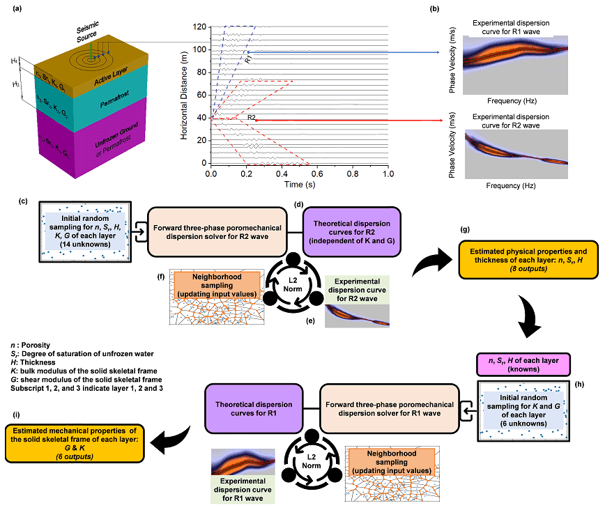
Figure 1 (a) A general schematic of the MASW test at a permafrost site. (b) Dispersion image of R1 and R2 waves obtained from the experimental measurements. (c) Initial guess of the physical properties of active layer, permafrost layer, and unfrozen ground. (d) Calculation of the theoretical dispersion relation of the R2 wave using the forward three-phase poromechanical dispersion solver. (e) Solution ranking based on L₂ norm for R2 dispersion relations (experimental versus theoretical) using the hybrid inverse and poromechanical approach. (f) Neighborhood sampling for the reduction in L₂ norm using the hybrid inverse and poromechanical approach. (g) Select the best samples based on the minimum L₂ norm and obtain the physical properties and thickness for each layer. (h) Repeat the steps for dispersion inversion (c–f) of R1 dispersion relation to derive the mechanical properties of active layer, permafrost layer, and unfrozen ground. (i) Select the best samples based on the minimum L₂ norm and obtain the mechanical properties.

2.2 Rayleigh wave dispersion relations

We consider the frozen soil specimen to be composed of three phases: solid skeletal frame, pore water, and pore ice. Through the infinitesimal kinematic assumption (Eq. C1), the stress–strain constitutive model (Carcione and Seriani, 2001) (Eq. C2), and the conservation of momentum (Eq. C3), the field equations can be written in the matrix form (Eq. C4). The matrices $\overline{\mathit{\rho }}$ , $\overline{\mathbf{b}}$, $\overline{\mathbf{R}}$, and $\overline{\mathit{\mu }}$ are given in Appendix D. The field equations can also be written in the frequency domain by performing convolution with e^iωt. The field equations in the Laplace domain are obtained by replacing ω with i⋅s ($i^{\mathrm{2}}=-\mathrm{1}$, and s is the Laplace variable).

To obtain the spectral element solution, the Helmholtz decomposition is used to decouple the P waves (P1, P2, and P3) and S waves (S1 and S2).

The displacement vector ($\overline{\mathit{u}}$) is composed of the P wave scalar potentials ϕ and S wave vector potentials $\overline{\mathit{\psi }}=({\mathit{\psi }}_r,{\mathit{\psi }}_{\mathit{\theta }},{\mathit{\psi }}_z)$. Since P waves exist in the solid skeleton, pore ice, and pore water phases, three P wave potentials are used, including ϕ_s, ϕ_i, and ϕ_f (Eq. C6).

The detailed steps for obtaining the closed-form solutions for P waves and S waves using the eigendecomposition are summarized in Appendix C. After obtaining the stiffness matrix for each layer, the global stiffness matrix, H, can be assembled by applying the continuity conditions at layer interfaces. The stiffness assembling method is shown in Fig. C1.

The dispersion relation of Rayleigh waves is obtained by setting a zero stress condition at the surface (z=0). To obtain the non-trivial solution, the determinant of the global stiffness matrix has to be zero, as expressed in Eq. (1) (Zomorodian and Hunaidi, 2006).

$$\begin{array}{}\text{(1)}& \det \mathbf{H}(\mathit{\omega },k)=\mathrm{0}\end{array}$$

The global stiffness matrix, H(ω,k), is a function of angular frequency ω and wavenumber k. For one given frequency, the value of the wavenumber can be determined when the determinant of the global stiffness matrix is zero. The dispersion curve is also commonly displayed as frequency versus phase velocity, $v=\frac{\mathit{\omega }}{k}$. The different wavenumbers determined at a given frequency correspond to dispersion curves of different modes. To extract the fundamental mode of the R1 wave, the velocities of the P1 wave and S1 wave are calculated first for the given physical properties and mechanical properties of each layer. The global stiffness matrix for the R1 wave can be decomposed into the components related only to the P1 and S1 wave velocities. This is viable since we have proved that the R1 wave is generated by the interaction between the P1 and S1 waves. This approach avoids the difficulties in differentiating the higher modes of the R2 wave from the fundamental mode of the R1 wave. An example is given in Appendix E to further explain and validate the decomposition of the global stiffness matrix. The detailed root search method has been documented in Liu et al. (2020b).

2.3 Inversion

The aim function is defined as the Euclidean norm between the experimental and numerical results of the dispersion relations. The problem is formulated in Eq. (2):

$$\begin{array}{}\text{(2)}& \left\{\begin{array}{l}\mathrm{minimize}{f}_{\left(x\right)}=\frac{\mathrm{1}}{\mathrm{2}}{\sum }_{i=\mathrm{1}}^N(y_i-{\overline{y}}_i(\mathit{x}){)}^{\mathrm{2}}\\ \mathrm{subject}\mathrm{to}{a}_i\le x_i\le b_i,i=\mathrm{1},\mathrm{\dots },m\end{array}\right.,\end{array}$$

where f is the objective function, $x=(x_{\mathrm{1}},x_{\mathrm{2}},\mathrm{\dots }{x}_m)$ is the optimization variable (e.g., porosity and degree of saturation of unfrozen water, bulk modulus and shear modulus of solid skeleton frame, and thickness of each layer), the constants a_i and b_i are limits or bounds for each variable, m is the total number of variables, and y and $\overline{y}$ are the numerical and experimental dispersion relations for the R1 or R2 waves.

In this paper, we used the neighborhood algorithm that benefits from the Voronoi cells to search the high-dimensional parameter space and reduce overall cost function (Sambridge, 1999). The algorithm contains only two tuning parameters (the number of samples and the number of resampled Voronoi cells) (Sambridge, 1999). The neighborhood sampling algorithm includes the following steps: a random sample is initially generated to ensure the soil parameters are not affected by the local minima. Based on the ranking of each sample, the Voronoi polygons are used to generate better samples with a smaller objective function. The optimization parameters are scaled between 0 and 1 to properly evaluate the Voronoi polygon limit. After generating a new sample, the distance calculation needs to be updated. Through enough iterations of these processes, the aim function can be reduced. The detailed description of the neighborhood algorithm is described by Sambridge (1999).

3 Identification of Rayleigh waves (R1 and R2) dispersion relations

From a poromechanical point of view, permafrost (frozen soil) is a multiphase porous medium that is composed of a solid skeletal frame and pores filled with water and ice in different proportions. Here, we analyze the seismic wave propagation in permafrost based on the three-phase poroelastodynamic theory. Three types of P wave (P1, P2, and P3) and two types of S wave (S1, S2) coexist in three-phase frozen porous media (Carcione et al., 2000; Carcione and Seriani, 2001; Carcione et al., 2003). The P1 and S1 waves are strongly related to the longitudinal and transverse waves propagating in the solid skeletal frame, respectively, but are also dependent on the interactions with pore ice and pore water (Carcione and Seriani, 2001). The P2 and S2 waves propagate mainly within pore ice (Leclaire et al., 1994). Similarly, the P3 wave is due to the interaction between the pore water and the solid skeletal frame. The velocity of different types of P waves and S waves is provided in Appendix A.

In this paper, a uniform frozen soil layer is used to show the propagation of different types of P and S waves and subsequently the formation of Rayleigh waves (R1 and R2) at the surface. It is assumed that an impulse load with a dominant frequency of 100 Hz is applied at the ground surface. The wave propagation analysis was performed in clayey soils by assuming a porosity (n) of 0.5, a degree of saturation of unfrozen water (Sr) of 50 %, a bulk modulus (K) of 20.9 GPa, and a shear modulus (G) of 6.85 GPa for the solid skeletal frame (Helgerud et al., 1999). The velocities of the P1 and P2 waves are calculated as 2628 and 910 m s⁻¹, respectively, based on the relations given in Appendix A. The velocity of the P3 wave (16 m s⁻¹) is relatively insignificant in comparison to P1 and P2 wave velocities. Similarly, the velocities of the S1 and S2 waves are calculated as 1217 and 481 m s⁻¹, respectively. Accordingly, the observed displacements measured at the ground surface with an offset from the impulse load ranging from 0 to 120 m are illustrated in Fig. 2a. We found that the velocities of R1 and R2 are 1150 and 450 m s⁻¹, respectively, using the three-phase dispersion relation derived in Sect. 2.2, which is exactly the same as what we captured in Fig. 2a. It is commonly known that the Rayleigh wave is slightly slower than the shear wave velocity, and the ratio of Rayleigh wave and shear wave velocity ranges from 0.92 to 0.95 for a Poisson ratio greater than 0.3 (Kazemirad and Mongeau, 2013). From this analysis, we found the ratio of R1 and S1 wave velocity is around 0.93. Similarly, the ratio of R2 and S2 wave velocity is around 0.94. Therefore, we can conclude that R1 waves appear due to the interaction of P1 and S1 waves since the phase velocity of R1 waves is slightly slower than the phase velocity of S1 waves. Similarly, R2 waves appear due to the interaction of P2 and S2 waves since the phase velocity of R2 waves is also slightly slower than the phase velocity of S2 waves. Figure 2b illustrates the waveforms of R1 and R2 waves at the offset of 80 m. It can be seen that the R1 and R2 waves have a much larger amplitude than any other components (e.g., P1, P2, S1, and S2), which is also consistent with the typical understanding of Rayleigh waves. Figure 2c and d illustrate the appearance of two types of Rayleigh waves (R1 and R2) in a three-phase permafrost subsurface at 70 and 100 ms, respectively. Our results convincingly demonstrate that R1 waves appear due to the interaction of P1 and S1 waves, and R2 waves appear due to the interaction of P2 and S2 waves. Briefly, the order of phase velocities of different waves propagating within the domain is as follows: P1>P2>S1>R1>S2>R2>P3.

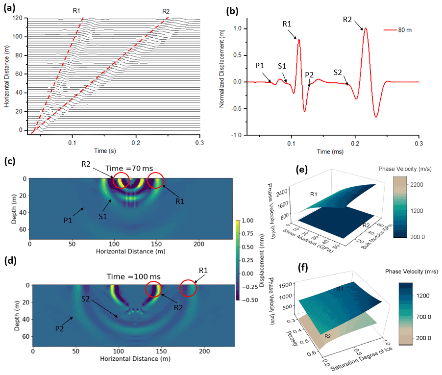
Figure 2 (a) Theoretical time-series measurements for R1 and R2 Rayleigh waves at the ground surface. (b) Waveforms of R1, R2, and other wave modes at the offset of 80 m. (c) Displacement contour at time 70 ms. (d) Displacement contour at time 100 ms with the labeled R1 and R2 Rayleigh waves. (e) Effect of shear modulus and bulk modulus of the solid skeletal frame on phase velocity of R1 and R2 waves. (f) Effect of degree of saturation of ice on the phase velocity of R1 and R2 waves.

The phase velocities of R1 and R2 waves are a function of physical properties (e.g., degree of saturation of unfrozen water, degree of saturation of ice, and porosity) and mechanical properties of the solid skeletal frame (e.g., bulk modulus and shear modulus). Figure 2d illustrates the effect of shear modulus and bulk modulus of the solid skeletal frame on the phase velocity of R1 and R2 waves. Similarly, Fig. 2e illustrates the effect of porosity and degree of saturation of ice on the phase velocity of R1 and R2 waves. It can be seen that the phase velocity of the R1 wave is mostly sensitive to the shear modulus of the solid skeletal frame; it is also dependent on the bulk modulus, porosity, and degree of saturation of ice. On the other hand, the phase velocity of the R2 wave is almost independent of the mechanical properties of the solid skeletal frame (Fig. 2d), while it is strongly affected by the porosity and degree of saturation of ice (Fig. 2e).

Our results also show that an increase in the degree of saturation of ice leads to an increase in the phase velocity of both types of Rayleigh waves. An increase in porosity leads to an increase in the phase velocity of R2. However, an increase in porosity may lead to either a decrease or an increase in the phase velocity of the R1 wave, depending on the level of the degree of saturation of ice. Hence, we use the phase velocity of R2 waves identified by processing the seismic surface wave measurements to characterize the physical properties (e.g., porosity, degree of saturation of ice, or degree of saturation of unfrozen water) of permafrost or soil layers.

4 Case study for the characterization of a permafrost site using a surface wave technique

The field experiment used in this study was performed by Glazer et al. (2020) who aimed to study the effect of nearby glacial ice and surface watercourses on the formation of different ice-bearing sediments (development of permafrost) within the late Quaternary marine terraces. In this paper, the same experimental data collected by Glazer et al. (2020) is used to demonstrate the inversion analysis based on R1 and R2 Rayleigh waves that we presented in Sect. 3. The case study site is located at the Fuglebekken coastal area in SW Spitsbergen, Svalbard (77${}^{\circ }{\mathrm{00}}^{\prime }{\mathrm{30}}^{\prime \prime }$ N, 15${}^{\circ }{\mathrm{33}}^{\prime }{\mathrm{00}}^{\prime \prime }$E). The study area has a thick layer of unconsolidated sediments that are suitable for near-surface geophysical investigations (Glazer et al., 2020). The unconsolidated sedimentary rock contains a high proportion of pore spaces; consequently, they can accumulate a large volume of pore water or pore ice. It was reported by Szymański et al. (2013) that this study site also contains a lot of coarse sandy soils and gravels based on the direct sampling methods at the top 15 cm. The direct sampling results also confirmed that the study site is very wet and the water table is very high (around 15 cm) (Szymański et al., 2013). From meteorological records, the mean annual air temperature (MAAT) at the testing site was historically below the freezing point, but more recently and due to a trend of climate warming, the MAAT recorded in 2016 is approaching 0 ^∘C (Glazer et al., 2020). Glazer et al. (2020) performed both seismic surveys (MASW test) and electrical resistivity investigations at the site in September 2017 to study the evolution and formation of permafrost considering surface watercourses and marine terrace. The MASW test was performed by using 60 geophone receivers with a frequency of 4.5 Hz spaced at regular 2 m intervals. Figure 3a shows the location of the test site. Figure 3b and c show the test site with different soil types (silty, clayey, and sandy sediment, as well as gravels). Figure 3e illustrates the collected original seismic measurements at distances between 0 and 120 m (hereafter referred to section 1). The R1 and R2 Rayleigh waves are identified to obtain the experimental dispersion relations (Fig. 3e and f). The phase velocity of the R1 wave increases with frequency from 24 to 80 Hz. The phase velocity of the R2 wave decreases with frequency in the span of 18 to 32 Hz. The largest wavelength is 22 m, calculated by the ratio of phase velocity of 404 m s⁻¹ and a frequency of 18 Hz. The investigation depth in this study is focused on the first 11 m (based on the recommendation that the MASW investigation depth is roughly half of the maximum wavelength (Olafsdottir et al., 2018).The uncertainties due to the selection of the dispersion curve from the dispersion spectra have been considered. The dispersion curve is automatically selected initially based on the highest intensity in the dispersion spectra using the “phase-shift method” in the MASWaves software (Olafsdottir et al., 2018). Then a 90 % confidence interval (labeled as lower bound, highest intensity, and upper bound, as shown in Fig. 3f and g) is considered to study the uncertainties of the selection of the dispersion curve to the inversion results.

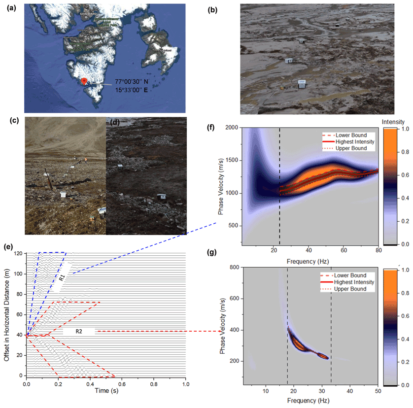
Figure 3 Surface wave measurement in section 1 (from 0 to 120 m). (a) Study area in Holocene, Fuglebekken, SW Spitsbergen (imagery source: © Google Earth, 77${}^{\circ }{\mathrm{00}}^{\prime }{\mathrm{30}}^{\prime \prime }$N and 15${}^{\circ }{\mathrm{33}}^{\prime }{\mathrm{00}}^{\prime \prime }$E). (b) Testing site with clayey silt soils. (c) Testing site with gravels and sands. (d) Testing site with patterned ground. (e) Waveform data from the measurements at different offsets in horizontal distance. (f) Experimental dispersion image for the R1 wave. (g) Experimental dispersion image for the R2 wave.

In our simulations, the permafrost site is modeled as a three-layered system, consisting of an active layer at the surface followed by a permafrost layer on top of the third layer (permafrost or unfrozen ground, which is to be determined). The ERT results reported by Glazer et al. (2020) proved that the active layer was most likely completely unfrozen during the MASW testing performed in September. The degree of saturation of unfrozen water is considered 100 % for the active layer in our study. The temperature of the permafrost layer remains below or at 0 ^∘C all year round, but the volumetric ice content of the test site is unknown. Therefore, in our simulation, the degree of saturation of unfrozen water in the permafrost layer is considered to be between 1 % and 85 % to be conservative. The degree of saturation of unfrozen water in the third layer is between 1 % and 100 % (permafrost or unfrozen ground, which is to be determined). In our study, the third layer is assumed to be infinite. However, with the limited investigation depth constrained by the wavelength of the MASW tests performed, the inversion results beyond the maximum investigation depth are not considered in the paper. The porosity of all three layers is distributed between 0.1 and 0.7. We previously showed that the dispersion relation of the R2 wave is strongly dependent on the physical properties (e.g., porosity and degree of saturation of unfrozen water). Hence, the R2 dispersion relation (Fig. 3d) is used first to determine the most probable distributions of porosity and degree of saturation of unfrozen water with depth. The other physical properties such as degree of saturation of ice, volumetric water content, and volumetric ice content can also be obtained by knowing porosity and degree of saturation of unfrozen water.

The mechanical properties of the solid skeletal frame in each layer are then obtained using the R1 wave dispersion relation. The mechanical properties can be then used to determine whether the permafrost site is ice-rich. In fact, the thin ice lenses can not be detected directly when the thickness of ice lenses is smaller than $\mathrm{1}/\mathrm{2}$ wavelength generated by low frequency seismic waves. However, the mechanical properties (e.g., shear modulus and bulk modulus) of permafrost reveal the mineral composition of the soil and soil type (Leclaire et al., 1994; Carcione and Seriani, 2001), which is valuable in the classification of ice-rich permafrost or even the detection of whether the permafrost layer is prone to greenhouse gas carbon dioxide and methane emission to the atmosphere.

Figure 4a shows the probabilistic distribution of the degree of saturation of unfrozen water with depth in section 1. Our results show that the active layer has a thickness of about 1.5 m. The predicted permafrost layer (second layer) has a nearly 32 % degree of saturation of unfrozen pore water. Figure 4b shows the degree of saturation of ice with depth. The degree of saturation of ice in the permafrost layer (second layer) ranges from 67 % to 71 %. Figure 4c illustrates the porosity distribution with depth. The porosity is around 0.60 in the first layer (active layer), from 0.40 to 0.47 in the second layer (permafrost), and from 0.56 to 0.59 in the third layer. Figure 4d and e show the predicted mechanical properties of the solid skeletal frame (shear modulus and bulk modulus) in each layer. It was reported by Szymański et al. (2013) that this study site also contains a lot of coarse sandy soils, gravels, and around 20 % silty clay based on the direct sampling methods at the top 15 cm. The predicted shear modulus and bulk modulus for the solid skeletal frame in the permafrost layer (second layer) are about 13 and 12.7 GPa, which are in the range for silty clay soils (Vanorio et al., 2003) and are also consistent with the local soil types described by Szymański et al. (2013). The predicted shear modulus and bulk modulus for the solid skeletal frame in the third layer are about 4 and 10 GPa, which are in the range for clayey soils (Vanorio et al., 2003). Figure 4f and g show the comparison between the numerical and experimental dispersion relations for R2 and R1 waves, respectively. The numerical predictions show good agreement with the experimental dispersion curves for both R1 (root mean square, RMS, value of 1.9) and R2 (RMS value of 4.7) waves.

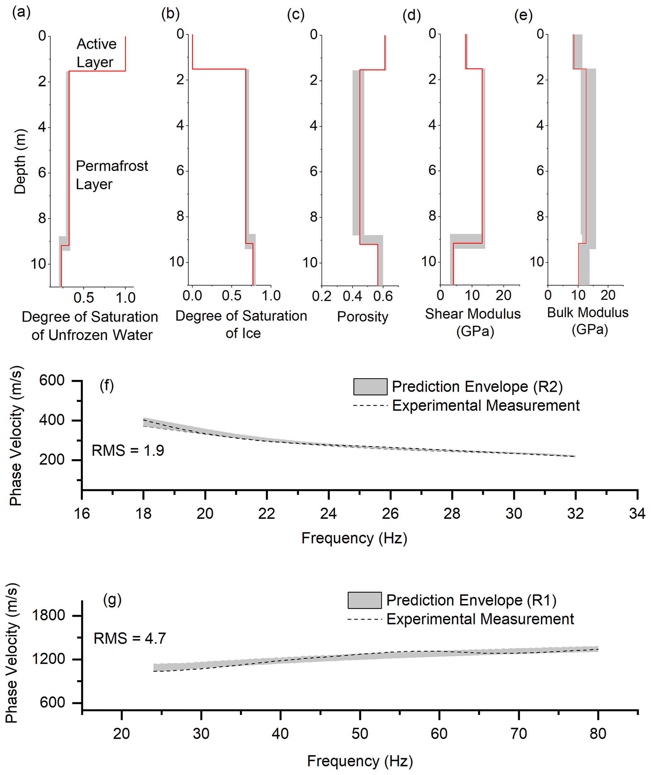
Figure 4 Surface wave inversion results for section 1: 0 to 120 m. (a) Degree of saturation of unfrozen water, (b) degree of saturation of ice, (c) porosity distribution, (d) shear modulus of solid skeletal frame, (e) bulk modulus of solid skeletal frame, (f) experimental and numerical dispersion curves for the R2 wave, and (g) experimental and numerical dispersion curves for the R1 wave.

Figure 5 illustrates the inversion process of the surface wave measurements for the R2 wave by means of the neighborhood algorithm. Initially, 20 random samples were employed in the entire space (to avoid the local minimum problem). Voronoi decomposition is used to generate representative sampling points about the best samples in the previous steps. Figure 5a shows the entire set of sampling points in the subspace between the porosity and the thickness of the active layer. Most sampling points are concentrated at the location where the porosity is 0.61 and the thickness of the active layer is 1.5 m. Similarly, in the subspace of the degree of saturation of unfrozen water and the porosity of the permafrost layer (second layer), our results show that the permafrost layer (second layer) most likely has a degree of saturation of unfrozen water of 32 % and a porosity of 0.44. Figure 5c shows the updates of each parameter (thickness, degree of saturation of unfrozen water, and porosity) with the number of the run in our forward solver. Our results show that the neighborhood algorithm fully explores the searching space of each parameter. Figure 5c also illustrates that the solution converged after roughly 4000 iterations, and the loss function (RMS) was reduced from 71 to only 1.9 at the end.

Figure 5 Inversion process for the R2 wave dispersion relation. (a) Sampling subspace between the degree of saturation of unfrozen water and the thickness of the active layer. (b) Sampling subspace between the degree of saturation of unfrozen water and the thickness of the permafrost layer. (c) Updates of thicknesses of the active layer and permafrost layer, as well as the physical properties in each layer by means of the neighborhood algorithm.

We have previously shown the inversion process and results for section 1 from 0 to 120 m. Five additional sections spanning from 120 to 600 m were also studied using a similar approach. The seismic measurements and dispersion relations for each section are given in Appendix B. Figure 6a shows the distribution of the degree of saturation of unfrozen water in the ground based on the five independent MASW tests. The result demonstrates that the permafrost table is generally located at about 1.5–1.9 m below the ground surface, which is consistent with the ERT results reported by Glazer et al. (2020) and results reported by Dolnicki et al. (2013) and Dobiński and Leszkiewicz (2010) using the direct probing method. Our inversion results showed that the porosity of the active layer ranges from 0.56 to 0.69, which is consistent with the field description by Glazer et al. (2020). The unfrozen water content in the second permafrost layer was predicted to range from 0.05 to 0.17. Li et al. (2020) and Zhang et al. (2020) showed that the residual volumetric unfrozen water content for silty clay, clay, medium sand, and fine sand is 0.12, 0.08, 0.06, and 0.03, respectively. Our inversion results predicted that permafrost (second layer) is mostly silty clay or clay (sections 1–3) and sandy soils, which are also consistent with the results described by Szymański et al. (2013). Figure 6e shows the variation in the shear modulus of the soil skeleton predicted by the proposed hybrid inverse and multiphase poromechanical approach. The predicted shear modulus in the first layer at the offset distance of 0 to 360 m ranges from 4 to 7.9 GPa, which represents clay soils (Helgerud et al., 1999). At the offset distance of 360 to 600 m, the estimated shear modulus in the first layer ranges from 27 to 33 GPa, which corresponds to soils with calcite constituents (Helgerud et al., 1999). Calcite most commonly occurs in sedimentary rock or gravels (Schmid et al., 1987), which is consistent with the field description given by Glazer et al. (2020) and Szymański et al. (2013). The higher value of shear wave velocity in sections 4 and 5 (spanning from 360 to 600 m, as shown in Fig. 6) is due to the higher value of the R1 wave dispersion curve. As shown in Fig. B5b, the dispersion curves of the R1 wave at sections 4 and 5 are relatively higher than those at the other three sections. The reason for a relatively higher R1 wave velocity in sections 4 and 5 could be the presence of the gravel or larger boulders, as discussed by Glazer et al. (2020) for the testing site.

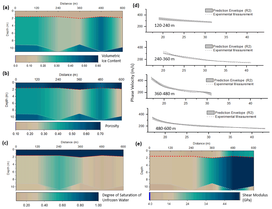
Figure 6 Summary of the inversion results at the offset distance from 0 m to 600 m. (a) Volumetric ice content distribution. (b) Soil porosity distribution. (c) Degree of saturation of unfrozen water distribution. (d) Comparison between the numerical and experimental dispersion curves for the R2 wave. (e) Distribution of the shear modulus of the solid skeleton.

5 Discussion and conclusions

We developed a hybrid inverse and multiphase poromechanical approach to quantitatively estimate the physical and mechanical properties of a permafrost site. The identification of two distinctive types of Rayleigh waves in the surface wave field measurements at permafrost sites is critical for the quantitative characterization of the layers. The identification of the R2 wave allows for the quantitative characterization of physical properties of soil layers independently without making assumptions of the mechanical properties of the layers. This approach simplifies the inversion of the multi-layered three-phase poromechanical model since the dependent optimization variables are largely reduced. The inversion results from the R2 wave dispersion relation can be further used in the characterization of the mechanical properties of soil layers based on the R1 wave dispersion relation. This also increases the stability and convergence rate of the inversion solver and makes the analysis more efficient than the joint inversion analysis.

Additional work on the characterization of permafrost should explore ways to reduce the uncertainty in the proposed hybrid inverse and multiphase poromechanical approach. The uncertainty originates from the non-uniqueness in the inverse analysis (local minima problem) and the limited number of constraints in the inversion analysis. It is recommended to use other geophysical methods to improve the resolution and reduce the uncertainty of the permafrost mapping. With the proposed seismic-wave-based method as the main investigation tool, ERT, GPR, and electromagnetic (EM) tomography can augment the investigation data and supply additional constraints to the inversion analysis.

In this paper, our results demonstrate the potential of seismic surface wave testing accompanied by our proposed hybrid inverse and poromechanical dispersion model for the assessment and quantitative characterization of permafrost sites. Its application for early detection and warning systems to monitor infrastructure impacted by permafrost-related geohazards and to detect the presence of layers vulnerable to permafrost carbon feedback and emission of greenhouse gases into the atmosphere will be the goal of our future studies. Currently, there is no advanced physics-based monitoring system developed for the real-time interpretation of seismic measurements. As such, active and passive seismic measurements can be collected and processed using the proposed hybrid inverse and poromechanical dispersion model for the assessment and quantitative characterization of permafrost sites at various depths in real time. In a future study, we will focus on the development of an early warning system for the long-term tracking of permafrost conditions. The early warning system can be used to collect seismic measurements and predict the physical and mechanical properties of the foundation permafrost. The system then reports periodic variations in physical (mostly ice content) and mechanical properties of the permafrost being monitored. The same method being applied on different dates (e.g., seasonal basis) can be used to record the change in properties of the permafrost site and then warn about the degradation of the permafrost exceeding the threshold. The determination of the value of the threshold (or critical values) will require more in-depth research. The early detection and warning systems can be beneficial in monitoring the condition of the foundation permafrost and preventing excessive thaw settlement and significant loss in strength. Similarly, we can detect the presence of peat (based on the physical and mechanical properties) which is vulnerable to permafrost carbon feedback and emission of greenhouse gases into the atmosphere. It is reported that the soils in the permafrost region hold twice as much carbon as the atmosphere does (almost 1600 billion tonnes) (Schuur et al., 2015). The thawing permafrost can rapidly trigger landslides and erosion. Current climate models assume that permafrost thaws gradually from the surface downwards (Schuur et al., 2015). However, several meters of soil can become destabilized within a few days or weeks instead of a few centimeters of permafrost thawing each year (Schuur et al., 2015). The missing element of the existing studies and models is that the abrupt permafrost destabilization can occur and contribute to more retrogressive thaw slumps and even carbon feedback. These features are not considered in existing models and hence cannot be predicted as the permafrost degrades.

Appendix A: Definition of phase velocities

The velocities of the three types of P waves are determined by a third-degree characteristic equation (Leclaire et al., 1994; Carcione et al., 2003).

$$\begin{array}{rl}{\mathrm{\Lambda }}^{\mathrm{3}}\stackrel{\mathrm{̃}}{R}& -{\mathrm{\Lambda }}^{\mathrm{2}}\left(\left({\mathit{\rho }}_{\mathrm{11}}{\stackrel{\mathrm{̃}}{R}}_{\mathrm{iw}}+{\mathit{\rho }}_{\mathrm{22}}{\stackrel{\mathrm{̃}}{R}}_{\mathrm{si}}\right.\right.\\ & \left.\left.+{\mathit{\rho }}_{\mathrm{33}}{\stackrel{\mathrm{̃}}{R}}_{\mathrm{sw}}\right)-\mathrm{2}\left(R_{\mathrm{11}}{R}_{\mathrm{33}}{\mathit{\rho }}_{\mathrm{23}}+R_{\mathrm{33}}{R}_{\mathrm{12}}{\mathit{\rho }}_{\mathrm{12}}\right)\right)\\ & +\mathrm{\Lambda }\left(\left(R_{\mathrm{11}}{\stackrel{\mathrm{̃}}{\mathit{\rho }}}_{\mathrm{iw}}+R_{\mathrm{22}}{\stackrel{\mathrm{̃}}{\mathit{\rho }}}_{\mathrm{si}}+R_{\mathrm{33}}{\stackrel{\mathrm{̃}}{\mathit{\rho }}}_{\mathrm{sw}}\right)\right.\\ & -\mathrm{2}\left.\left({\mathit{\rho }}_{\mathrm{11}}{\mathit{\rho }}_{\mathrm{23}}{R}_{\mathrm{23}}+{\mathit{\rho }}_{\mathrm{33}}{\mathit{\rho }}_{\mathrm{12}}{R}_{\mathrm{12}}\right)\right)-\stackrel{\mathrm{̃}}{\mathit{\rho }}=\mathrm{0},\end{array}$$

where

$$\begin{array}{c}{\displaystyle }\stackrel{\mathrm{̃}}{R}=R_{\mathrm{11}}{R}_{\mathrm{22}}{R}_{\mathrm{33}}-R_{\mathrm{23}}^{\mathrm{2}}{R}_{\mathrm{11}}-R_{\mathrm{12}}^{\mathrm{2}}{R}_{\mathrm{33}}\\ {\displaystyle }{\stackrel{\mathrm{̃}}{R}}_{\mathrm{sw}}=R_{\mathrm{11}}{R}_{\mathrm{22}}-R_{\mathrm{12}}^{\mathrm{2}}\\ {\displaystyle }{\stackrel{\mathrm{̃}}{R}}_{\mathrm{iw}}=R_{\mathrm{22}}{R}_{\mathrm{33}}-R_{\mathrm{23}}^{\mathrm{2}}\\ {\displaystyle }{\stackrel{\mathrm{̃}}{R}}_{\mathrm{si}}=R_{\mathrm{11}}{R}_{\mathrm{33}}\\ {\displaystyle }\stackrel{\mathrm{̃}}{\mathit{\rho }}={\mathit{\rho }}_{\mathrm{11}}{\mathit{\rho }}_{\mathrm{22}}{\mathit{\rho }}_{\mathrm{33}}-{\mathit{\rho }}_{\mathrm{23}}^{\mathrm{2}}{\mathit{\rho }}_{\mathrm{11}}-{\mathit{\rho }}_{\mathrm{12}}^{\mathrm{2}}{\mathit{\rho }}_{\mathrm{33}}\\ {\displaystyle }{\stackrel{\mathrm{̃}}{\mathit{\rho }}}_{\mathrm{sw}}={\mathit{\rho }}_{\mathrm{11}}{\mathit{\rho }}_{\mathrm{22}}-{\mathit{\rho }}_{\mathrm{12}}^{\mathrm{2}}\\ {\displaystyle }{\stackrel{\mathrm{̃}}{\mathit{\rho }}}_{\mathrm{iw}}={\mathit{\rho }}_{\mathrm{22}}{\mathit{\rho }}_{\mathrm{33}}-{\mathit{\rho }}_{\mathrm{23}}^{\mathrm{2}}\\ {\displaystyle }{\stackrel{\mathrm{̃}}{\mathit{\rho }}}_{\mathrm{si}}={\mathit{\rho }}_{\mathrm{11}}{\mathit{\rho }}_{\mathrm{33}}.\end{array}$$

The roots of the third-degree characteristic equation, denoted as Λ₁, Λ₂, and Λ₃, can be found by computing the eigenvalues of the companion matrix (Horn and Johnson, 2012). The velocities of the three types of P wave (v_P1>v_P2>v_P3) are given as follows:

$${\displaystyle }{\displaystyle }{v}_{\mathrm{P}\mathrm{1}}=\sqrt{{\displaystyle \frac{\mathrm{1}}{{\mathrm{\Lambda }}_{\mathrm{1}}}}};{\displaystyle }{v}_{\mathrm{P}\mathrm{2}}=\sqrt{{\displaystyle \frac{\mathrm{1}}{{\mathrm{\Lambda }}_{\mathrm{2}}}}};{\displaystyle }{v}_{\mathrm{P}\mathrm{3}}=\sqrt{{\displaystyle \frac{\mathrm{1}}{{\mathrm{\Lambda }}_{\mathrm{3}}}}}.$$

The velocities of the two types of S wave are determined by a second-degree characteristic equation:

$${\displaystyle }{\mathit{\delta }}^{\mathrm{2}}{\mathit{\rho }}_{\mathrm{22}}{\stackrel{\mathrm{̃}}{\mathit{\mu }}}_{\mathrm{si}}-\mathit{\delta }({\mathit{\mu }}_{\mathrm{11}}{\stackrel{\mathrm{̃}}{\mathit{\rho }}}_{\mathrm{iw}}+{\mathit{\mu }}_{\mathrm{33}}{\stackrel{\mathrm{̃}}{\mathit{\rho }}}_{\mathrm{sw}})+\stackrel{\mathrm{̃}}{\mathit{\rho }}=\mathrm{0}.$$

The roots of this second-degree characteristic equation are denoted by δ₁ and δ₂. The velocities of the two types of S wave (v_S1>v_S2) are given as follows:

$${\displaystyle }{\displaystyle }{v}_{\mathrm{S}\mathrm{1}}=\sqrt{{\displaystyle \frac{\mathrm{1}}{{\mathit{\delta }}_{\mathrm{1}}}}},{\displaystyle }{v}_{\mathrm{S}\mathrm{2}}=\sqrt{{\displaystyle \frac{\mathrm{1}}{{\mathit{\delta }}_{\mathrm{2}}}}}.$$

Appendix B: Inversion results for other sections

The inversion results for the sections ranging from 120 to 600 m are summarized in Fig. B1 to B4.

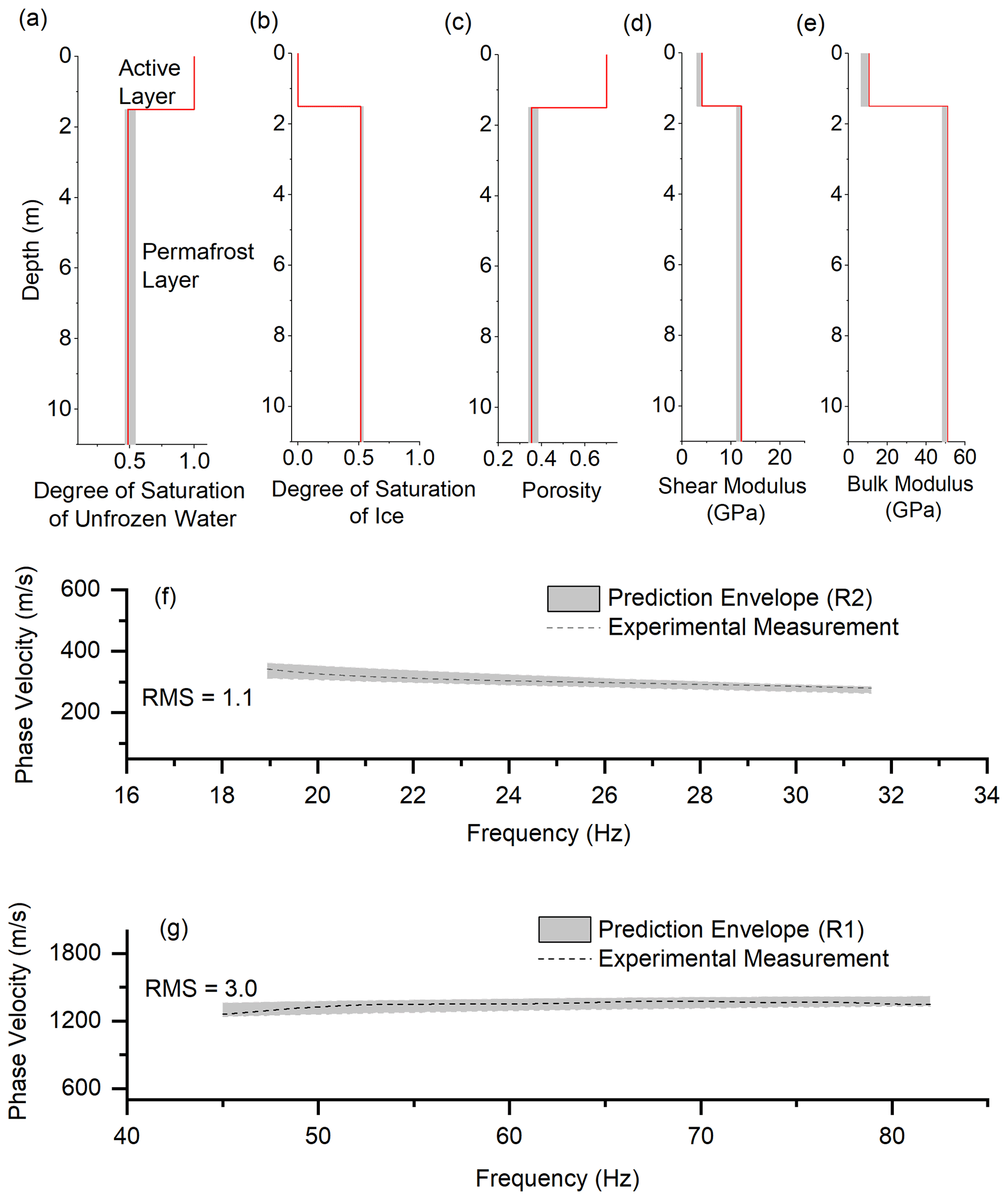
Figure B1 Surface wave inversion results for section 2: 120 to 240 m. (a) Degree of saturation of unfrozen water, (b) degree of saturation of ice, (c) porosity distribution, (d) shear modulus of solid skeletal frame, (e) bulk modulus of solid skeletal frame, (f) experimental and numerical dispersion curves for the R2 wave, and (g) experimental and numerical dispersion curves for the R1 wave.

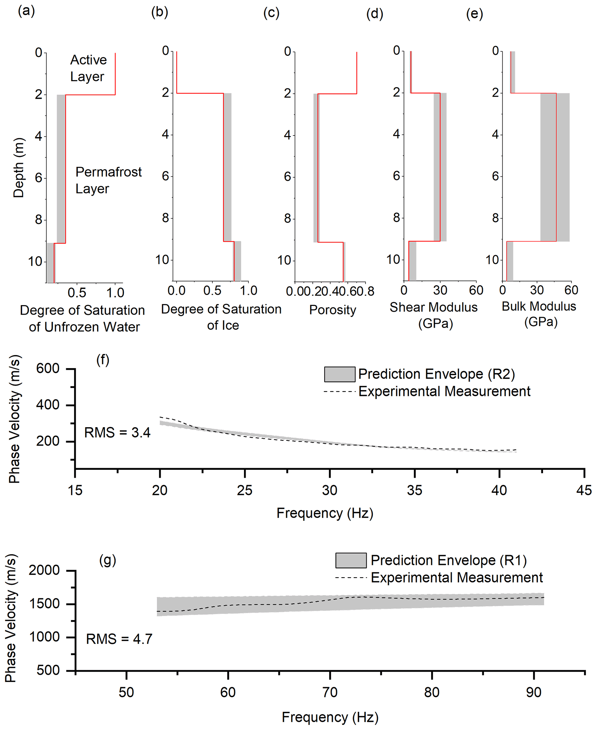
Figure B2 Surface wave inversion results for section 3: 240 to 360 m. (a) Degree of saturation of unfrozen water, (b) degree of saturation of ice, (c) porosity distribution, (d) shear modulus of solid skeletal frame, (e) bulk modulus of solid skeletal frame, (f) experimental and numerical dispersion curves for the R2 wave, and (g) experimental and numerical dispersion curves for the R1 wave.

Figure B3 Surface wave inversion results for section 4 (from 360 to 480 m). (a) Degree of saturation of unfrozen water, (b) degree of saturation of ice, (c) porosity distribution, (d) shear modulus of solid skeletal frame, (e) bulk modulus of solid skeletal frame, (f) experimental and numerical dispersion curves for the R2 wave, and (g) experimental and numerical dispersion curves for the R1 wave.

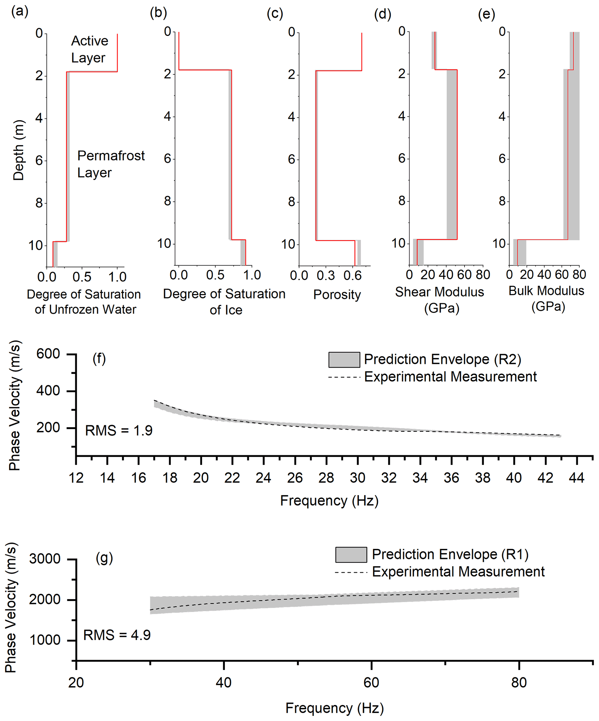
Figure B4 Surface wave inversion results for section 5 (from 480 to 600 m). (a) Degree of saturation of unfrozen water, (b) degree of saturation of ice, (c) porosity distribution, (d) shear modulus of solid skeletal frame, (e) bulk modulus of solid skeletal frame, (f) experimental and numerical dispersion curves for the R2 wave, and (g) experimental and numerical dispersion curves for the R1 wave.

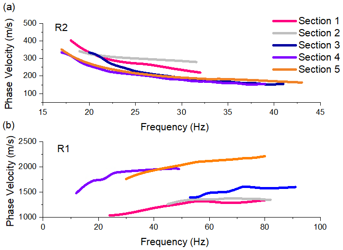
Figure B5 Summary of dispersion measurements for sections 1 to 5. (a) Dispersion curves of the R2 wave. (b) Dispersion curves of the R1 wave.

Appendix C: Forward three-phase poromechanical model

Kinematics assumptions

The Green–Lagrange strain tensor (ϵ_ij) for infinitesimal deformations expressed as displacement vector u¹, u², and u³ for the solid skeleton, pore water, and pore ice, respectively, are shown in Eq. (C1) (Leclaire et al., 1994; Carcione et al., 2003).

$$\begin{array}{}\text{(C1)}& \left\{\begin{array}{l}{\mathit{ϵ}}_{\mathrm{ij}}^{\mathrm{1}}=\frac{\mathrm{1}}{\mathrm{2}}(u_{i,j}^{\mathrm{1}}+u_{j,i}^{\mathrm{1}})\\ {\mathit{ϵ}}_{\mathrm{ij}}^{\mathrm{2}}=\frac{\mathrm{1}}{\mathrm{3}}{\mathit{ϵ}}_{\mathrm{kk}}^{\mathrm{2}}{\mathit{\delta }}_{\mathrm{ij}}({\mathit{ϵ}}_{\mathrm{kk}}^{\mathrm{2}}=u_{k,k}^{\mathrm{2}})\\ {\mathit{ϵ}}_{\mathrm{ij}}^{\mathrm{3}}=\frac{\mathrm{1}}{\mathrm{2}}(u_{i,j}^{\mathrm{3}}+u_{j,i}^{\mathrm{3}})\end{array}\right.,\end{array}$$

where δ_ij is the identity tensor.

The strain tensor of pore water ${\mathit{ϵ}}_{\mathrm{ij}}^{\mathrm{2}}$ is diagonal since the shear deformation does not exist in the pore water component.

Constitutive model

The constitutive models defined as the relation between the stress and strain tensors for solid skeleton, pore water, and pore ice are given in Eq. (C2) (Leclaire et al., 1994; Carcione et al., 2003).

$$\begin{array}{}\text{(C2)}& \left\{\begin{array}{l}{\mathit{\sigma }}_{\mathrm{ij}}^{\mathrm{1}}=(K_{\mathrm{1}}{\mathit{\theta }}_{\mathrm{1}}+C_{\mathrm{12}}{\mathit{\theta }}_{\mathrm{2}}+C_{\mathrm{13}}{\mathit{\theta }}_{\mathrm{3}}){\mathit{\delta }}_{\mathrm{ij}}+\mathrm{2}{\mathit{\mu }}_{\mathrm{1}}{d}_{\mathrm{ij}}^{\mathrm{1}}+{\mathit{\mu }}_{\mathrm{13}}{d}_{\mathrm{ij}}^{\mathrm{3}}\\ {\mathit{\sigma }}^{\mathrm{2}}=C_{\mathrm{12}}{\mathit{\theta }}_{\mathrm{1}}+K_{\mathrm{2}}{\mathit{\theta }}_{\mathrm{2}}+C_{\mathrm{23}}{\mathit{\theta }}_{\mathrm{3}}\\ {\mathit{\sigma }}_{\mathrm{ij}}^{\mathrm{3}}=(K_{\mathrm{3}}{\mathit{\theta }}_{\mathrm{3}}+C_{\mathrm{23}}{\mathit{\theta }}_{\mathrm{2}}+C_{\mathrm{13}}{\mathit{\theta }}_{\mathrm{1}}){\mathit{\delta }}_{\mathrm{ij}}+\mathrm{2}{\mathit{\mu }}_{\mathrm{3}}{d}_{\mathrm{ij}}^{\mathrm{3}}+{\mathit{\mu }}_{\mathrm{13}}{d}_{\mathrm{ij}}^{\mathrm{1}}\end{array}\right.,\end{array}$$

in which σ¹, σ², and σ³ are the effective stress, pore water pressure, and ice pressure, respectively. The definition of each term (e.g., K₁, C₁₂, C₁₃, μ₁, μ₁₃, K₂, C₂₃, K₃, μ₃) in Eq. (C2) is given in Appendix D. The terms θ_m, $d_{\mathrm{ij}}^m$, and ${\mathit{ϵ}}_{\mathrm{ij}}^m$ (m, ranging from 1 to 3, represents the different phases) are defined as follows:

$$\left\{\begin{array}{l}{\mathit{\theta }}_m={\mathit{ϵ}}_{\mathrm{kk}}^m\\ d_{\mathrm{ij}}^m={\mathit{ϵ}}_{\mathrm{ij}}^m-\frac{\mathrm{1}}{\mathrm{3}}{\mathit{\delta }}_{\mathrm{ij}}{\mathit{\theta }}_m\\ {\mathit{ϵ}}_{\mathrm{ij}}^m=\frac{\mathrm{1}}{\mathrm{2}}(u_{i,j}^m+u_{j,i}^m)\end{array}\right..$$

Conservation laws

The momentum conservation considers the acceleration of each component and the existing relative motion of the pore ice and pore water phases with respect to the solid skeleton. The momentum conservation for the three phases is given by Eq. (C3) (Leclaire et al., 1994; Carcione et al., 2003).

$$\begin{array}{}\text{(C3)}& \left\{\begin{array}{l}{\mathit{\sigma }}_{\mathrm{ij},j}^{\mathrm{1}}={\mathit{\rho }}_{\mathrm{11}}{\ddot{u}}_i^{\mathrm{1}}+{\mathit{\rho }}_{\mathrm{12}}{\ddot{u}}_i^{\mathrm{2}}+{\mathit{\rho }}_{\mathrm{13}}{\ddot{u}}_i^{\mathrm{3}}-b_{\mathrm{12}}({\dot{u}}_i^{\mathrm{2}}-{\dot{u}}_i^{\mathrm{1}})-b_{\mathrm{13}}({\dot{u}}_i^{\mathrm{3}}-{\dot{u}}_i^{\mathrm{1}})\\ {\mathit{\sigma }}_{,i}^{\mathrm{2}}={\mathit{\rho }}_{\mathrm{12}}{\ddot{u}}_i^{\mathrm{1}}+{\mathit{\rho }}_{\mathrm{22}}{\ddot{u}}_i^{\mathrm{2}}+{\mathit{\rho }}_{\mathrm{23}}{\ddot{u}}_i^{\mathrm{3}}+b_{\mathrm{12}}({\dot{u}}_i^{\mathrm{2}}-{\dot{u}}_i^{\mathrm{1}})+b_{\mathrm{23}}({\dot{u}}_i^{\mathrm{2}}-{\dot{u}}_i^{\mathrm{3}})\\ {\mathit{\sigma }}_{\mathrm{ij},j}^{\mathrm{3}}={\mathit{\rho }}_{\mathrm{13}}{\ddot{u}}_i^{\mathrm{1}}+{\mathit{\rho }}_{\mathrm{23}}{\ddot{u}}_i^{\mathrm{2}}+{\mathit{\rho }}_{\mathrm{33}}{\ddot{u}}_i^{\mathrm{3}}-b_{\mathrm{23}}({\dot{u}}_i^{\mathrm{2}}-{\dot{u}}_i^{\mathrm{1}})+b_{\mathrm{13}}({\dot{u}}_i^{\mathrm{3}}-{\dot{u}}_i^{\mathrm{1}})\end{array}\right.,\end{array}$$

in which the expressions for the density terms (ρ_ij or $\overline{\mathit{\rho }}$ in matrix form) and viscous matrix (b_ij or $\overline{\mathbf{b}}$ in matrix form) are given in Appendix D, $\ddot{u}$ and $\dot{u}$ represent second and first derivatives of displacement vectors with respect to time, and the subscript i represents the component in r, θ, and z directions in cylindrical coordinates.

Through the infinitesimal kinematic assumptions, the stress–strain constitutive model, and conversation of momentum, the field equation can be written in the matrix form, as shown in Eq. (C4).

$$\begin{array}{}\text{(C4)}& \overline{\mathit{\rho }}\left[\begin{array}{c}{\ddot{u}}_i^{\mathrm{1}}\\ {\ddot{u}}_i^{\mathrm{2}}\\ {\ddot{u}}_i^{\mathrm{3}}\end{array}\right]+\overline{\mathbf{b}}\left[\begin{array}{c}{\dot{u}}_i^{\mathrm{1}}\\ {\dot{u}}_i^{\mathrm{2}}\\ {\dot{u}}_i^{\mathrm{3}}\end{array}\right]=\overline{\mathbf{R}}\mathrm{\nabla }\mathrm{\nabla }\cdot \left[\begin{array}{c}{u}_i^{\mathrm{1}}\\ u_i^{\mathrm{2}}\\ u_i^{\mathrm{3}}\end{array}\right]-\overline{\mathit{\mu }}\mathrm{\nabla }\times \mathrm{\nabla }\times \left[\begin{array}{c}{u}_i^{\mathrm{1}}\\ u_i^{\mathrm{2}}\\ u_i^{\mathrm{3}}\end{array}\right],\end{array}$$

in which the matrices $\overline{\mathbf{R}}$ and $\overline{\mathit{\mu }}$ are given in Appendix D.

By performing divergence operation (∇⋅) and curl operation (∇×) on both sides of Eq. (C4), the field equation in the frequency domain can be written as Eq. (C5).

$$\begin{array}{}\text{(C5)}& \left\{\begin{array}{l}-\overline{\mathit{\rho }}{\mathit{\omega }}^{\mathrm{2}}\mathrm{\nabla }\cdot \left[\begin{array}{c}{u}_i^{\mathrm{1}}\\ u_i^{\mathrm{2}}\\ u_i^{\mathrm{3}}\end{array}\right]-\overline{\mathbf{b}}i\mathit{\omega }\mathrm{\nabla }\cdot \left[\begin{array}{c}{u}_i^{\mathrm{1}}\\ u_i^{\mathrm{2}}\\ u_i^{\mathrm{3}}\end{array}\right]=\overline{\mathbf{R}}{\mathrm{\nabla }}^{\mathrm{2}}\mathrm{\nabla }\cdot \left[\begin{array}{c}{u}_i^{\mathrm{1}}\\ u_i^{\mathrm{2}}\\ u_i^{\mathrm{3}}\end{array}\right]\\ -\overline{\mathit{\rho }}{\mathit{\omega }}^{\mathrm{2}}\mathrm{\nabla }\times \left[\begin{array}{c}{u}_i^{\mathrm{1}}\\ u_i^{\mathrm{2}}\\ u_i^{\mathrm{3}}\end{array}\right]-\overline{\mathbf{b}}i\mathit{\omega }\mathrm{\nabla }\times \left[\begin{array}{c}{u}_i^{\mathrm{1}}\\ u_i^{\mathrm{2}}\\ u_i^{\mathrm{3}}\end{array}\right]=\overline{\mathit{\mu }}{\mathrm{\nabla }}^{\mathrm{2}}\mathrm{\nabla }\times \left[\begin{array}{c}{u}_i^{\mathrm{1}}\\ u_i^{\mathrm{2}}\\ u_i^{\mathrm{3}}\end{array}\right]\end{array}\right.\end{array}$$

Using the Helmholtz decomposition theorem allows us to decompose the displacement field, $\overline{u}$ (equivalent to u_i), into the longitudinal potential and transverse vector components as follows:

$$\begin{array}{}\text{(C6)}& \left\{\begin{array}{l}{\overline{u}}^{\mathrm{1}}=\mathrm{\nabla }{\mathit{\varphi }}_{\mathrm{1}}+\mathrm{\nabla }\times {\overline{\mathit{\psi }}}_{\mathrm{1}}\mathrm{and}\mathrm{\nabla }\cdot {\overline{\mathit{\psi }}}_{\mathrm{1}}=\mathrm{0}\\ {\overline{u}}^{\mathrm{2}}=\mathrm{\nabla }{\mathit{\varphi }}_{\mathrm{2}}+\mathrm{\nabla }\times {\overline{\mathit{\psi }}}_{\mathrm{2}}\mathrm{and}\mathrm{\nabla }\cdot {\overline{\mathit{\psi }}}_{\mathrm{2}}=\mathrm{0}\\ {\overline{u}}^{\mathrm{3}}=\mathrm{\nabla }{\mathit{\varphi }}_{\mathrm{3}}+\mathrm{\nabla }\times {\overline{\mathit{\psi }}}_{\mathrm{3}}\mathrm{and}\mathrm{\nabla }\cdot {\overline{\mathit{\psi }}}_{\mathrm{3}}=\mathrm{0}\end{array}\right..\end{array}$$

By substituting Eq. (C6) into the field equation of motion, Eq. (C5), we obtain two sets of uncoupled partial differential equations relative to the compressional P wave related to the Helmholtz scalar potentials and to the shear S wave related to the Helmholtz vector potential (Eq. C7). In the axisymmetric condition, only the second components exist in vector $\overline{\mathit{\psi }}$, which is denoted as ψ in the future. It should be mentioned that the field equations in the Laplace domain can be easily obtained by replacing ω with i⋅s ($i^{\mathrm{2}}=-\mathrm{1}$, and s is the Laplace variable).

$$\begin{array}{}\text{(C7)}& \left\{\begin{array}{l}-\overline{\mathit{\rho }}{\mathit{\omega }}^{\mathrm{2}}\left[\begin{array}{c}{\mathit{\varphi }}_{\mathrm{1}}\\ {\mathit{\varphi }}_{\mathrm{2}}\\ {\mathit{\varphi }}_{\mathrm{3}}\end{array}\right]-\overline{\mathbf{b}}i\mathit{\omega }\left[\begin{array}{c}{\mathit{\varphi }}_{\mathrm{1}}\\ {\mathit{\varphi }}_{\mathrm{2}}\\ {\mathit{\varphi }}_{\mathrm{3}}\end{array}\right]=\overline{\mathbf{R}}{\mathrm{\nabla }}^{\mathrm{2}}\left[\begin{array}{c}{\mathit{\varphi }}_{\mathrm{1}}\\ {\mathit{\varphi }}_{\mathrm{2}}\\ {\mathit{\varphi }}_{\mathrm{3}}\end{array}\right]\\ -\overline{\mathit{\rho }}{\mathit{\omega }}^{\mathrm{2}}\left[\begin{array}{c}{\mathit{\psi }}_{\mathrm{1}}\\ {\mathit{\psi }}_{\mathrm{2}}\\ {\mathit{\psi }}_{\mathrm{3}}\end{array}\right]-\overline{\mathbf{b}}i\mathit{\omega }\left[\begin{array}{c}{\mathit{\psi }}_{\mathrm{1}}\\ {\mathit{\psi }}_{\mathrm{2}}\\ {\mathit{\psi }}_{\mathrm{3}}\end{array}\right]=\overline{\mathit{\mu }}{\mathrm{\nabla }}^{\mathrm{2}}\left[\begin{array}{c}{\mathit{\psi }}_{\mathrm{1}}\\ {\mathit{\psi }}_{\mathrm{2}}\\ {\mathit{\psi }}_{\mathrm{3}}\end{array}\right]\end{array}\right.\end{array}$$

Solution for the longitudinal waves (P waves) by eigendecomposition

Equation (C7) shows that ϕ₁, ϕ₂, and ϕ₃ are coupled in the field equations. The diagonalization of such a matrix is required to decouple the system. Equation (C7) is then rearranged into Eq. (C8).

$$\begin{array}{}\text{(C8)}& {\mathrm{\nabla }}^{\mathrm{2}}\left[\begin{array}{c}{\mathit{\varphi }}_{\mathrm{1}}\\ {\mathit{\varphi }}_{\mathrm{2}}\\ {\mathit{\varphi }}_{\mathrm{3}}\end{array}\right]=\underset{\overline{\mathbf{K}}}{\underbrace{-{\overline{\mathbf{R}}}^{-\mathrm{1}}(\overline{\mathit{\rho }}{\mathit{\omega }}^{\mathrm{2}}+\overline{\mathbf{b}}i\mathit{\omega })}}\left[\begin{array}{c}{\mathit{\varphi }}_{\mathrm{1}}\\ {\mathit{\varphi }}_{\mathrm{2}}\\ {\mathit{\varphi }}_{\mathrm{3}}\end{array}\right],\end{array}$$

where the $\overline{\mathbf{K}}$ matrix can be rewritten using the eigendecomposition:

$$\begin{array}{}\text{(C9)}& \overline{\mathbf{K}}=\overline{\mathit{P}}\overline{\mathbf{D}}{\overline{\mathit{P}}}^{-\mathrm{1}},\end{array}$$

where $\overline{\mathit{P}}$ is the eigenvector, and $\overline{\mathbf{D}}$ is the eigenvalue matrix of $\overline{\mathbf{K}}$.

By setting $\overline{\mathit{\varphi }}=\overline{\mathit{P}}\overline{y}$, where $\overline{\mathit{y}}=[{\mathit{\varphi }}_{\mathrm{P}\mathrm{1}},{\mathit{\varphi }}_{\mathrm{P}\mathrm{2}},{\mathit{\varphi }}_{\mathrm{P}\mathrm{3}}]$, we can obtain ${\mathrm{\nabla }}^{\mathrm{2}}\overline{y}=\overline{\mathbf{D}}\overline{\mathit{y}}$. The equation of the longitudinal wave has been decoupled. In cylindrical coordinates, the solution for $\overline{\mathit{y}}=[{\mathit{\varphi }}_{\mathrm{P}\mathrm{1}},{\mathit{\varphi }}_{\mathrm{P}\mathrm{2}},{\mathit{\varphi }}_{\mathrm{P}\mathrm{3}}]$ is summarized as follows:

$$\begin{array}{}\text{(C10)}& \left\{\begin{array}{l}{\mathit{\varphi }}_{\mathrm{P}\mathrm{1}}(r,z)=A{e}^{-\sqrt{k^{\mathrm{2}}+D_{\mathrm{11}}}z}{J}_{\mathrm{0}}\left(kr\right)\\ {\mathit{\varphi }}_{\mathrm{P}\mathrm{2}}(r,z)=B{e}^{-\sqrt{k^{\mathrm{2}}+D_{\mathrm{22}}}z}{J}_{\mathrm{0}}\left(kr\right)\\ {\mathit{\varphi }}_{\mathrm{P}\mathrm{3}}(r,z)=C{e}^{-\sqrt{k^{\mathrm{2}}+D_{\mathrm{33}}}z}{J}_{\mathrm{0}}\left(kr\right)\end{array}\right.,\end{array}$$

where k is the wave number; coefficients A, B, and C will be determined by boundary conditions; D₁₁, D₂₂, and D₃₃ are the diagonal components of $\overline{\mathbf{D}}$; and J₀ is the Bessel function of the first kind. For simplicity, the terms $\sqrt{k^{\mathrm{2}}+D_{\mathrm{11}}}$, $\sqrt{k^{\mathrm{2}}+D_{\mathrm{22}}}$, and $\sqrt{k^{\mathrm{2}}+D_{\mathrm{33}}}$ are denoted as k_P1, k_P2, and k_P3, respectively.

Now, the P wave potentials can be written as follows:

$$\begin{array}{}\text{(C11)}& {\displaystyle }\left\{\begin{array}{c}{\mathit{\varphi }}_s\\ {\mathit{\varphi }}_w\\ {\mathit{\varphi }}_i\end{array}\right\}=\left\{\begin{array}{ccc}{p}_{\mathrm{11}}& p_{\mathrm{12}}& p_{\mathrm{13}}\\ p_{\mathrm{21}}& p_{\mathrm{22}}& p_{\mathrm{23}}\\ p_{\mathrm{31}}& p_{\mathrm{32}}& p_{\mathrm{33}}\end{array}\right\}\left\{\begin{array}{c}{\mathit{\varphi }}_{\mathrm{P}\mathrm{1}}\\ {\mathit{\varphi }}_{\mathrm{P}\mathrm{2}}\\ {\mathit{\varphi }}_{\mathrm{P}\mathrm{3}}\end{array}\right\},\end{array}$$

where p_ij are the components for the eigenvector of $\overline{\mathit{P}}$.

Solution for shear waves (S waves)

The solutions for the S wave potentials can be solved in a similar manner. Eq. (C12) is firstly rearranged into Eq. C13.

$$\begin{array}{}\text{(C12)}& -\overline{\mathit{\rho }}{\mathit{\omega }}^{\mathrm{2}}\left[\begin{array}{c}{\mathit{\psi }}_s\\ {\mathit{\psi }}_w\\ {\mathit{\psi }}_i\end{array}\right]-\overline{\mathbf{b}}i\mathit{\omega }\left[\begin{array}{c}{\mathit{\psi }}_s\\ {\mathit{\psi }}_w\\ {\mathit{\psi }}_i\end{array}\right]=\overline{\mathit{\mu }}{\mathrm{\nabla }}^{\mathrm{2}}\left[\begin{array}{c}{\mathit{\psi }}_s\\ {\mathit{\psi }}_w\\ {\mathit{\psi }}_i\end{array}\right],\end{array}$$

$$\begin{array}{}\text{(C13)}& \underset{\overline{\mathbf{A}}}{\underbrace{-\overline{\mathit{\rho }}{\mathit{\omega }}^{\mathrm{2}}-\overline{\mathbf{b}}i\mathit{\omega }}}\left[\begin{array}{c}{\mathit{\psi }}_s\\ {\mathit{\psi }}_w\\ {\mathit{\psi }}_i\end{array}\right]=\overline{\mathit{\mu }}{\mathrm{\nabla }}^{\mathrm{2}}\left[\begin{array}{c}{\mathit{\psi }}_s\\ {\mathit{\psi }}_w\\ {\mathit{\psi }}_i\end{array}\right],\end{array}$$

where the matrix $\overline{\mathbf{A}}$ is given in Appendix D.

Since ψ_w can be expressed as a function of ψ_s and ψ_i (shown in Eq. C14), Eq. (C13) is further simplified and rearranged into Eq. (C15).

$$\begin{array}{}\text{(C14)}& \left\{\begin{array}{l}{A}_{\mathrm{21}}{\mathit{\psi }}_s+A_{\mathrm{22}}{\mathit{\psi }}_w+A_{\mathrm{23}}{\mathit{\psi }}_i=\mathrm{0}\\ {\mathit{\psi }}_w=-\frac{A_{\mathrm{21}}{\mathit{\psi }}_s+A_{\mathrm{23}}{\mathit{\psi }}_i}{A_{\mathrm{22}}}\end{array}\right.,\end{array}$$

$$\begin{array}{}\text{(C15)}& {\mathrm{\nabla }}^{\mathrm{2}}\left[\begin{array}{c}{\mathit{\psi }}_s\\ {\mathit{\psi }}_i\end{array}\right]=\underset{\overline{\mathbf{N}}}{\underbrace{{\left[\begin{array}{cc}{\mathit{\mu }}_{\mathrm{11}}& {\mathit{\mu }}_{\mathrm{13}}\\ {\mathit{\mu }}_{\mathrm{13}}& {\mathit{\mu }}_{\mathrm{33}}\end{array}\right]}^{-\mathrm{1}}\overline{C}}}\left[\begin{array}{c}{\mathit{\psi }}_s\\ {\mathit{\psi }}_i\end{array}\right],\end{array}$$

where

$$\overline{C}=\left(\begin{array}{cc}{A}_{\mathrm{11}}-\frac{A_{\mathrm{12}}{A}_{\mathrm{21}}}{A_{\mathrm{22}}}& A_{\mathrm{13}}-\frac{A_{\mathrm{12}}{A}_{\mathrm{23}}}{A_{\mathrm{22}}}\\ A_{\mathrm{31}}-\frac{A_{\mathrm{32}}{A}_{\mathrm{21}}}{A_{\mathrm{22}}}& A_{\mathrm{33}}-\frac{A_{\mathrm{32}}{A}_{\mathrm{23}}}{A_{\mathrm{22}}}\end{array}\right).$$

The $\overline{\mathbf{N}}$ matrix can be rewritten using the eigendecomposition ($\overline{\mathbf{N}}=\overline{\mathit{Q}}\overline{\mathbf{G}}{\overline{\mathit{Q}}}^{-\mathrm{1}}$), where $\overline{\mathit{Q}}$ is the eigenvector, and $\overline{\mathbf{G}}$ is the eigenvalue matrix of $\overline{\mathbf{N}}$. By setting $\overline{\mathit{\psi }}=\overline{\mathit{Q}}\overline{y^{\prime }}$, where $\overline{y^{\prime }}=[{\mathit{\psi }}_{\mathrm{S}\mathrm{1}},{\mathit{\psi }}_{i\mathrm{1}}]$, we can obtain the following:

$$\begin{array}{}\text{(C16)}& \begin{array}{rl}& {\mathit{\psi }}_{\mathrm{S}\mathrm{1}}=E{e}^{-\sqrt{k^{\mathrm{2}}+G_{\mathrm{11}}z}}{J}_{\mathrm{1}}\left(kr\right),\\ & {\mathit{\psi }}_{i\mathrm{1}}=F{e}^{-\sqrt{k^{\mathrm{2}}+G_{\mathrm{22}}z}}{J}_{\mathrm{1}}\left(kr\right),\end{array}\end{array}$$

where J₁ is the Bessel function of the first kind with order 1. G₁₁ and G₂₂ are the diagonal components of matrix $\overline{\mathbf{G}}$. For simplicity, the terms $\sqrt{k^{\mathrm{2}}+G_{\mathrm{11}}}$ and $\sqrt{k^{\mathrm{2}}+G_{\mathrm{22}}}$ are denoted as k_S1 and k_S2.

Finally, the solution of the S wave potentials can be written as follows:

$$\begin{array}{}\text{(C17)}& {\displaystyle }\left\{\begin{array}{c}{\mathit{\psi }}_s\\ {\mathit{\psi }}_i\end{array}\right\}=\left\{\begin{array}{cc}{Q}_{\mathrm{11}}& Q_{\mathrm{12}}\\ Q_{\mathrm{21}}& Q_{\mathrm{22}}\end{array}\right\}\left\{\begin{array}{c}{\mathit{\psi }}_{\mathrm{S}\mathrm{1}}\\ {\mathit{\psi }}_{i\mathrm{1}}\end{array}\right\},\end{array}$$

where Q_ij are the components for eigenvector of $\overline{\mathit{Q}}$.

Layer element with finite thickness

By including both incident wave and reflected wave, the potentials for a layer with finite thickness can be written as in Eq. (C18):

$$\begin{array}{}\text{(C18)}& \left[\begin{array}{c}{u}_{r\mathrm{1}}^{\mathrm{1}}\\ u_{z\mathrm{1}}^{\mathrm{1}}\\ u_{z\mathrm{1}}^{\mathrm{2}}\\ u_{r\mathrm{1}}^{\mathrm{3}}\\ u_{z\mathrm{1}}^{\mathrm{3}}\\ u_{r\mathrm{2}}^{\mathrm{1}}\\ u_{z\mathrm{2}}^{\mathrm{1}}\\ u_{z\mathrm{2}}^{\mathrm{2}}\\ u_{r\mathrm{2}}^{\mathrm{3}}\\ u_{z\mathrm{2}}^{\mathrm{3}}\end{array}\right]=\left[\begin{array}{cccccc}& & & & & \\ & & & & & \\ & & & & & \\ & & & & & \\ & & & & & {\mathbf{S}}_{\mathrm{1}}\\ & & & & & \\ & & & & & \\ & & & & & \\ & & & & & \\ & & & & & \end{array}\right]\left[\begin{array}{c}{A}_{\mathrm{1}}\\ B_{\mathrm{1}}\\ C_{\mathrm{1}}\\ E_{\mathrm{1}}\\ F_{\mathrm{1}}\\ A_{\mathrm{2}}\\ B_{\mathrm{2}}\\ C_{\mathrm{2}}\\ E_{\mathrm{2}}\\ F_{\mathrm{2}}\end{array}\right],\end{array}$$

where the components of S₁ are given in Appendix F, and the subscripts 1 and 2 represent the nodes for the upper and lower layers, respectively. The coefficients A to F are determined by the boundary condition.

The matrix of effective stress, pore water pressure, and pore ice pressure in the frequency domain is shown in Eq. (C19) in which the components for matrix S₂ can be found in Appendix F.

$$\begin{array}{}\text{(C19)}& \left[\begin{array}{c}{\mathit{\sigma }}_{r\mathrm{1}}^{\mathrm{1}}\\ {\mathit{\sigma }}_{z\mathrm{1}}^{\mathrm{1}}\\ p_{\mathrm{1}}\\ {\mathit{\sigma }}_{r\mathrm{1}}^{\mathrm{3}}\\ {\mathit{\sigma }}_{z\mathrm{1}}^{\mathrm{3}}\\ {\mathit{\sigma }}_{r\mathrm{2}}^{\mathrm{1}}\\ {\mathit{\sigma }}_{z\mathrm{2}}^{\mathrm{1}}\\ p_{\mathrm{2}}\\ {\mathit{\sigma }}_{r\mathrm{2}}^{\mathrm{3}}\\ {\mathit{\sigma }}_{z\mathrm{2}}^{\mathrm{3}}\end{array}\right]=\left[\begin{array}{cccccc}& & & & & \\ & & & & & \\ & & & & & \\ & & & & & \\ & & & & & {\mathbf{S}}_{\mathrm{2}}\\ & & & & & \\ & & & & & \\ & & & & & \\ & & & & & \\ & & & & & \end{array}\right]\left[\begin{array}{c}{A}_{\mathrm{1}}\\ B_{\mathrm{1}}\\ C_{\mathrm{1}}\\ E_{\mathrm{1}}\\ F_{\mathrm{1}}\\ A_{\mathrm{2}}\\ B_{\mathrm{2}}\\ C_{\mathrm{2}}\\ E_{\mathrm{2}}\\ F_{\mathrm{2}}\end{array}\right]\end{array}$$

According to the Cauchy stress principle, the traction force (T) is taken as the dot product between the stress tensor and the unit vector along the outward normal direction. Due to the convention that the upward direction is negative, the upper boundary becomes negative. Similarly, to make the sign consistent, the N matrix is applied to matrix ${\mathbf{S}}_{\mathrm{2}}\cdot {\mathbf{S}}_{\mathrm{1}}^{-\mathrm{1}}$. In the future, the matrix $\mathbf{N}\cdot {\mathbf{S}}_{\mathrm{2}}\cdot {\mathbf{S}}_{\mathrm{1}}^{-\mathrm{1}}$ will be denoted as the G_i matrix, in which i denotes the layer number.

$$\begin{array}{}\text{(C20)}& {\displaystyle }{\left[\begin{array}{c}{T}_{r\mathrm{1}}^{\mathrm{1}}\\ T_{z\mathrm{1}}^{\mathrm{1}}\\ T_{\mathrm{1}}\\ T_{r\mathrm{1}}^{\mathrm{3}}\\ T_{z\mathrm{1}}^{\mathrm{3}}\\ T_{r\mathrm{2}}^{\mathrm{1}}\\ T_{z\mathrm{2}}^{\mathrm{1}}\\ T_{\mathrm{2}}\\ T_{r\mathrm{2}}^{\mathrm{3}}\\ T_{z\mathrm{2}}^{\mathrm{3}}\end{array}\right]}_i={\left[\begin{array}{c}-{\mathit{\sigma }}_{r\mathrm{1}}^{\mathrm{1}}\\ -{\mathit{\sigma }}_{z\mathrm{1}}^{\mathrm{1}}\\ -p_{\mathrm{1}}\\ -{\mathit{\sigma }}_{r\mathrm{1}}^{\mathrm{3}}\\ -{\mathit{\sigma }}_{z\mathrm{1}}^{\mathrm{3}}\\ {\mathit{\sigma }}_{r\mathrm{2}}^{\mathrm{1}}\\ {\mathit{\sigma }}_{z\mathrm{2}}^{\mathrm{1}}\\ p_{\mathrm{2}}\\ {\mathit{\sigma }}_{r\mathrm{2}}^{\mathrm{3}}\\ {\mathit{\sigma }}_{z\mathrm{2}}^{\mathrm{3}}\end{array}\right]}_i=\underset{{\mathbf{G}}_i}{\underbrace{\mathbf{N}\cdot {\mathbf{S}}_{\mathrm{2}}\cdot {\mathbf{S}}_{\mathrm{1}}^{-\mathrm{1}}}}\cdot {\left[\begin{array}{c}{u}_{r\mathrm{1}}^{\mathrm{1}}\\ u_{z\mathrm{1}}^{\mathrm{1}}\\ u_{z\mathrm{1}}^{\mathrm{2}}\\ u_{r\mathrm{1}}^{\mathrm{3}}\\ u_{z\mathrm{1}}^{\mathrm{3}}\\ u_{r\mathrm{2}}^{\mathrm{1}}\\ u_{z\mathrm{2}}^{\mathrm{1}}\\ u_{z\mathrm{2}}^{\mathrm{2}}\\ u_{r\mathrm{2}}^{\mathrm{3}}\\ u_{z\mathrm{2}}^{\mathrm{3}}\end{array}\right]}_i,\end{array}$$

where

$$\begin{array}{}\text{(C21)}& {\displaystyle }\mathbf{N}=\left[\begin{array}{cccccccccc}-\mathrm{1}& \mathrm{0}& \mathrm{0}& \mathrm{0}& \mathrm{0}& \mathrm{0}& \mathrm{0}& \mathrm{0}& \mathrm{0}& \mathrm{0}\\ \mathrm{0}& -\mathrm{1}& \mathrm{0}& \mathrm{0}& \mathrm{0}& \mathrm{0}& \mathrm{0}& \mathrm{0}& \mathrm{0}& \mathrm{0}\\ \mathrm{0}& \mathrm{0}& -\mathrm{1}& \mathrm{0}& \mathrm{0}& \mathrm{0}& \mathrm{0}& \mathrm{0}& \mathrm{0}& \mathrm{0}\\ \mathrm{0}& \mathrm{0}& \mathrm{0}& -\mathrm{1}& \mathrm{0}& \mathrm{0}& \mathrm{0}& \mathrm{0}& \mathrm{0}& \mathrm{0}\\ \mathrm{0}& \mathrm{0}& \mathrm{0}& \mathrm{0}& -\mathrm{1}& \mathrm{0}& \mathrm{0}& \mathrm{0}& \mathrm{0}& \mathrm{0}\\ \mathrm{0}& \mathrm{0}& \mathrm{0}& \mathrm{0}& \mathrm{0}& \mathrm{1}& \mathrm{0}& \mathrm{0}& \mathrm{0}& \mathrm{0}\\ \mathrm{0}& \mathrm{0}& \mathrm{0}& \mathrm{0}& \mathrm{0}& \mathrm{0}& \mathrm{1}& \mathrm{0}& \mathrm{0}& \mathrm{0}\\ \mathrm{0}& \mathrm{0}& \mathrm{0}& \mathrm{0}& \mathrm{0}& \mathrm{0}& \mathrm{0}& \mathrm{1}& \mathrm{0}& \mathrm{0}\\ \mathrm{0}& \mathrm{0}& \mathrm{0}& \mathrm{0}& \mathrm{0}& \mathrm{0}& \mathrm{0}& \mathrm{0}& \mathrm{1}& \mathrm{0}\\ \mathrm{0}& \mathrm{0}& \mathrm{0}& \mathrm{0}& \mathrm{0}& \mathrm{0}& \mathrm{0}& \mathrm{0}& \mathrm{0}& \mathrm{1}\end{array}\right].\end{array}$$

Layer element with infinite thickness

By assuming that no wave reflects back to a semi-infinite element, a one-node element with infinite thickness is applied. The matrix for the displacement components in the one-node layer is written as Eq. (C22). The matrix S₁ is reduced into a 5 by 5 matrix (S_1ij, where i and j range from 1 to 5). The values of each component are shown in Appendix F.

$$\begin{array}{}\text{(C22)}& \left[\begin{array}{c}{u}_{r\mathrm{1}}^{\mathrm{1}}\\ u_{z\mathrm{1}}^{\mathrm{1}}\\ u_{z\mathrm{1}}^{\mathrm{2}}\\ u_{r\mathrm{1}}^{\mathrm{3}}\\ u_{z\mathrm{1}}^{\mathrm{3}}\end{array}\right]=\left[\begin{array}{ccc}& & \\ & & \\ & & {\mathbf{S}}_{\mathrm{1}}\\ & & \end{array}\right]\left[\begin{array}{c}{A}_{\mathrm{1}}\\ B_{\mathrm{1}}\\ C_{\mathrm{1}}\\ E_{\mathrm{1}}\\ F_{\mathrm{1}}\end{array}\right]\end{array}$$

Similarly, the matrix of effective stress components and porewater pressure in the frequency domain is shown in Eq. (C23). The matrix S₂ is reduced into a 5 by 5 matrix (S_2ij, where i and j range from 1 to 5). The matrix G_h in Fig. C1 is calculated as ${\mathbf{G}}_h={\mathbf{S}}_{\mathrm{2}}{\mathbf{S}}_{\mathrm{1}}^{-\mathrm{1}}$. The values of each component are shown in Appendix F.

$$\begin{array}{}\text{(C23)}& \left[\begin{array}{c}{\mathit{\sigma }}_{r\mathrm{1}}^{\mathrm{1}}\\ {\mathit{\sigma }}_{z\mathrm{1}}^{\mathrm{1}}\\ p_{\mathrm{1}}\\ {\mathit{\sigma }}_{r\mathrm{1}}^{\mathrm{3}}\\ {\mathit{\sigma }}_{z\mathrm{1}}^{\mathrm{3}}\end{array}\right]=\left[\begin{array}{ccc}& & \\ & & \\ & & {\mathbf{S}}_{\mathrm{2}}\\ & & \end{array}\right]\left[\begin{array}{c}{A}_{\mathrm{1}}\\ B_{\mathrm{1}}\\ C_{\mathrm{1}}\\ E_{\mathrm{1}}\\ F_{\mathrm{1}}\end{array}\right]\end{array}$$

The stiffness assembling method is shown in Fig. C1.

Figure C1 Construction of the global stiffness matrix in which G is the stiffness matrix of a layer, the h represents the number of layers with finite thickness, and the m represents the half-space layer.

Appendix D: Parameter definitions

The matrices $\overline{\mathit{\rho }}$, $\overline{\mathbf{b}}$, $\overline{\mathbf{R}}$, $\overline{\mathit{\mu }}$, and $\overline{\mathbf{A}}$ are defined as follows (Leclaire et al., 1994; Carcione et al., 2003).

$$\overline{\mathit{\rho }}=\left[\begin{array}{ccc}{\mathit{\rho }}_{\mathrm{11}}& {\mathit{\rho }}_{\mathrm{12}}& {\mathit{\rho }}_{\mathrm{13}}\\ {\mathit{\rho }}_{\mathrm{12}}& {\mathit{\rho }}_{\mathrm{22}}& {\mathit{\rho }}_{\mathrm{23}}\\ {\mathit{\rho }}_{\mathrm{13}}& {\mathit{\rho }}_{\mathrm{23}}& {\mathit{\rho }}_{\mathrm{33}}\end{array}\right]\overline{\mathbf{b}}=\left[\begin{array}{ccc}{b}_{\mathrm{12}}+b_{\mathrm{13}}& -b_{\mathrm{12}}& -b_{\mathrm{13}}\\ -b_{\mathrm{12}}& b_{\mathrm{12}}+b_{\mathrm{23}}& -b_{\mathrm{23}}\\ -b_{\mathrm{13}}& -b_{\mathrm{23}}& b_{\mathrm{13}}+b_{\mathrm{23}}\end{array}\right]$$

$$\overline{\mathbf{R}}=\left[\begin{array}{ccc}{R}_{\mathrm{11}}& R_{\mathrm{12}}& R_{\mathrm{13}}\\ R_{\mathrm{12}}& R_{\mathrm{22}}& R_{\mathrm{23}}\\ R_{\mathrm{13}}& R_{\mathrm{23}}& R_{\mathrm{33}}\end{array}\right]\overline{\mathit{\mu }}=\left[\begin{array}{ccc}{\mathit{\mu }}_{\mathrm{11}}& \mathrm{0}& {\mathit{\mu }}_{\mathrm{13}}\\ \mathrm{0}& \mathrm{0}& \mathrm{0}\\ {\mathit{\mu }}_{\mathrm{13}}& \mathrm{0}& {\mathit{\mu }}_{\mathrm{33}}\end{array}\right]$$

$$\begin{array}{ll}{\displaystyle }& {\displaystyle }\overline{\mathbf{A}}=\\ {\displaystyle }& {\displaystyle }-\left(\begin{array}{ccc}\mathit{\omega }\left(\right(b_{\mathrm{12}}+b_{\mathrm{13}})i+{\mathit{\rho }}_{\mathrm{11}}\mathit{\omega })& \mathit{\omega }({\mathit{\rho }}_{\mathrm{12}}\mathit{\omega }-b_{\mathrm{12}}i)& \mathit{\omega }({\mathit{\rho }}_{\mathrm{13}}\mathit{\omega }-b_{\mathrm{13}}i)\\ \mathit{\omega }({\mathit{\rho }}_{\mathrm{12}}\mathit{\omega }-b_{\mathrm{12}}i)& \mathit{\omega }\left(\right(b_{\mathrm{12}}+b_{\mathrm{23}})i+{\mathit{\rho }}_{\mathrm{22}}\mathit{\omega })& \mathit{\omega }({\mathit{\rho }}_{\mathrm{23}}\mathit{\omega }-b_{\mathrm{23}}i)\\ \mathit{\omega }({\mathit{\rho }}_{\mathrm{13}}\mathit{\omega }-b_{\mathrm{13}}i)& \mathit{\omega }({\mathit{\rho }}_{\mathrm{23}}\mathit{\omega }-b_{\mathrm{23}}i)& \mathit{\omega }\left(\right(b_{\mathrm{13}}+b_{\mathrm{23}})i+{\mathit{\rho }}_{\mathrm{33}}\mathit{\omega })\end{array}\right)\end{array}$$

$$\begin{array}{c}{\displaystyle }{a}_{\mathrm{12}}=r_{\mathrm{12}}{\displaystyle \frac{{\mathit{\varphi }}_s({\mathit{\varphi }}_w{\mathit{\rho }}_w+{\mathit{\varphi }}_i{\mathit{\rho }}_i)}{{\mathit{\varphi }}_w{\mathit{\rho }}_w({\mathit{\varphi }}_w+{\mathit{\varphi }}_i)}}+\mathrm{1}\\ {\displaystyle }{a}_{\mathrm{23}}=r_{\mathrm{23}}{\displaystyle \frac{{\mathit{\varphi }}_s({\mathit{\varphi }}_w{\mathit{\rho }}_w+{\mathit{\varphi }}_s{\mathit{\rho }}_s)}{{\mathit{\varphi }}_w{\mathit{\rho }}_w({\mathit{\varphi }}_w+{\mathit{\varphi }}_s)}}+\mathrm{1}\\ {\displaystyle }{a}_{\mathrm{13}}=r_{\mathrm{13}}{\displaystyle \frac{{\mathit{\varphi }}_i({\mathit{\varphi }}_s{\mathit{\rho }}_s+{\mathit{\varphi }}_i{\mathit{\rho }}_i)}{{\mathit{\varphi }}_s{\mathit{\rho }}_s({\mathit{\varphi }}_s+{\mathit{\varphi }}_i)}}+\mathrm{1}\\ {\displaystyle }{a}_{\mathrm{31}}=r_{\mathrm{31}}{\displaystyle \frac{{\mathit{\varphi }}_s({\mathit{\varphi }}_s{\mathit{\rho }}_s+{\mathit{\varphi }}_i{\mathit{\rho }}_i)}{{\mathit{\varphi }}_i{\mathit{\rho }}_i({\mathit{\varphi }}_s+{\mathit{\varphi }}_i)}}+\mathrm{1}\\ {\displaystyle }{\mathit{\rho }}_{\mathrm{11}}=a_{\mathrm{13}}{\mathit{\varphi }}_s{\mathit{\rho }}_s+(a_{\mathrm{12}}-\mathrm{1}){\mathit{\varphi }}_w{\mathit{\rho }}_w+(a_{\mathrm{31}}-\mathrm{1}){\mathit{\varphi }}_i{\mathit{\rho }}_i\\ {\displaystyle }{\mathit{\rho }}_{\mathrm{22}}=(a_{\mathrm{12}}+a_{\mathrm{23}}-\mathrm{1}){\mathit{\varphi }}_w{\mathit{\rho }}_w\\ {\displaystyle }{\mathit{\rho }}_{\mathrm{33}}=(a_{\mathrm{13}}-\mathrm{1}){\mathit{\varphi }}_s{\mathit{\rho }}_s+(a_{\mathrm{23}}-\mathrm{1}){\mathit{\varphi }}_w{\mathit{\rho }}_w+a_{\mathrm{31}}{\mathit{\varphi }}_i{\mathit{\rho }}_i\\ {\displaystyle }{\mathit{\rho }}_{\mathrm{12}}=-(a_{\mathrm{12}}-\mathrm{1}){\mathit{\varphi }}_w{\mathit{\rho }}_w\\ {\displaystyle }{\mathit{\rho }}_{\mathrm{13}}=-(a_{\mathrm{13}}-\mathrm{1}){\mathit{\varphi }}_s{\mathit{\rho }}_s-(a_{\mathrm{31}}-\mathrm{1}){\mathit{\varphi }}_i{\mathit{\rho }}_i\\ {\displaystyle }{\mathit{\rho }}_{\mathrm{23}}=-(a_{\mathrm{23}}-\mathrm{1}){\mathit{\varphi }}_w{\mathit{\rho }}_w\\ {\displaystyle }\begin{array}{rl}{b}_{\mathrm{12}}={\mathit{\eta }}_w{\mathit{\varphi }}_w^{\mathrm{2}}/{\mathit{\kappa }}_s:& \text{friction coefficient between the solid skeletal}\\ & \text{frame and pore water}\end{array}\\ {\displaystyle }\begin{array}{rl}{b}_{\mathrm{23}}={\mathit{\eta }}_w{\mathit{\varphi }}_w^{\mathrm{2}}/{\mathit{\kappa }}_i:& \text{friction coefficient between pore water and}\\ & \text{ice matrix}\end{array}\\ {\displaystyle }\begin{array}{rl}{b}_{\mathrm{13}}=b_{\mathrm{13}}^{\mathrm{0}}({\mathit{\varphi }}_i{\mathit{\varphi }}_s{)}^{\mathrm{2}}:& \text{friction coefficient between the solid}\\ & \text{skeletal frame and ice matrix}\end{array}\\ {\displaystyle }{\mathit{\kappa }}_s={\mathit{\kappa }}_{s\mathrm{0}}{s}_r^{\mathrm{3}}\\ {\displaystyle }{\mathit{\kappa }}_i={\mathit{\kappa }}_{i\mathrm{0}}{\mathit{\varphi }}^{\mathrm{3}}/\left[(\mathrm{1}-s_r^{\mathrm{2}})(\mathrm{1}-\mathit{\varphi }{)}^{\mathrm{3}}\right]\\ {\displaystyle }{R}_{\mathrm{11}}={\left[(\mathrm{1}-c_{\mathrm{1}}){\mathit{\varphi }}_s\right]}^{\mathrm{2}}{K}_{\mathrm{av}}+K_{\mathrm{sm}}+\mathrm{4}{\mathit{\mu }}_{\mathrm{11}}/\mathrm{3}\\ {\displaystyle }{R}_{\mathrm{22}}={\mathit{\varphi }}_w^{\mathrm{2}}{K}_{\mathrm{av}}\\ {\displaystyle }{R}_{\mathrm{33}}={\left[(\mathrm{1}-c_{\mathrm{3}}){\mathit{\varphi }}_i\right]}^{\mathrm{2}}{K}_{\mathrm{av}}+K_{\mathrm{im}}+\mathrm{4}{\mathit{\mu }}_{\mathrm{33}}/\mathrm{3}\\ {\displaystyle }{R}_{\mathrm{12}}=(\mathrm{1}-c_{\mathrm{1}}){\mathit{\varphi }}_s{\mathit{\varphi }}_w{K}_{\mathrm{av}}\\ {\displaystyle }{R}_{\mathrm{13}}=(\mathrm{1}-c_{\mathrm{1}})(\mathrm{1}-c_{\mathrm{3}}){\mathit{\varphi }}_s{\mathit{\varphi }}_i{K}_{\mathrm{av}}+\mathrm{2}{\mathit{\mu }}_{\mathrm{13}}/\mathrm{3}\\ {\displaystyle }{R}_{\mathrm{23}}=(\mathrm{1}-c_{\mathrm{3}}){\mathit{\varphi }}_w{\mathit{\varphi }}_i{K}_{\mathrm{av}}\\ {\displaystyle }{\mathit{\mu }}_{\mathrm{11}}={\left[(\mathrm{1}-g_{\mathrm{1}}){\mathit{\varphi }}_s\right]}^{\mathrm{2}}{\mathit{\mu }}_{\mathrm{av}}+{\mathit{\mu }}_{\mathrm{sm}}\\ {\displaystyle }{\mathit{\mu }}_{\mathrm{33}}={\left[(\mathrm{1}-g_{\mathrm{3}}){\mathit{\varphi }}_i\right]}^{\mathrm{2}}{\mathit{\mu }}_{\mathrm{av}}+{\mathit{\mu }}_{\mathrm{im}}\\ {\displaystyle }{\mathit{\mu }}_{\mathrm{13}}=(\mathrm{1}-g_{\mathrm{1}})(\mathrm{1}-g_{\mathrm{3}}){\mathit{\mu }}_{\mathrm{av}}\\ {\displaystyle }\begin{array}{rl}{c}_{\mathrm{1}}=K_{\mathrm{sm}}/\left({\mathit{\varphi }}_s{K}_s\right):& \text{consolidation coefficient for the solid}\\ & \text{skeletal frame}\end{array}\\ {\displaystyle }{c}_{\mathrm{3}}=K_{\mathrm{im}}/\left({\mathit{\varphi }}_i{K}_i\right):\text{consolidation coefficient for the ice}\\ {\displaystyle }{g}_{\mathrm{1}}={\mathit{\mu }}_{\mathrm{sm}}/\left({\mathit{\varphi }}_s{\mathit{\mu }}_s\right)\\ {\displaystyle }{g}_{\mathrm{3}}={\mathit{\mu }}_{\mathrm{im}}/\left({\mathit{\varphi }}_i{\mathit{\mu }}_i\right)\\ {\displaystyle }\begin{array}{rl}{K}_{\mathrm{im}}={\mathit{\varphi }}_i{K}_i/\left[\mathrm{1}+\mathit{\alpha }(\mathrm{1}-{\mathit{\varphi }}_i)\right]:& \text{bulk modulus of the matrix}\\ & \text{formed by the ice}\end{array}\\ {\displaystyle }\begin{array}{rl}{\mathit{\mu }}_{\mathrm{im}}={\mathit{\varphi }}_i{\mathit{\mu }}_i/\left[\mathrm{1}+\mathit{\alpha }\mathit{\gamma }(\mathrm{1}-{\mathit{\varphi }}_i)\right]:& \text{shear modulus of the matrix}\\ & \text{formed by the ice}\end{array}\\ {\displaystyle }\begin{array}{rl}{K}_{\mathrm{sm}}=(\mathrm{1}-{\mathit{\varphi }}_w-\overline{\mathit{\xi }}{\mathit{\varphi }}_i)K_s/\left[\mathrm{1}+\mathit{\alpha }({\mathit{\varphi }}_w+\overline{\mathit{\xi }}{\mathit{\varphi }}_i)\right]:& \text{bulk modulus}\\ & \text{of the solid}\\ & \text{skeletal frame}\end{array}\\ {\displaystyle }\begin{array}{rl}{\mathit{\mu }}_{\mathrm{sm}}=(\mathrm{1}-{\mathit{\varphi }}_w-\overline{\mathit{\xi }}{\mathit{\varphi }}_i){\mathit{\mu }}_s/\left[\mathrm{1}+\mathit{\alpha }\mathit{\gamma }({\mathit{\varphi }}_w+\overline{\mathit{\xi }}{\mathit{\varphi }}_i)\right]:& \text{shear modulus}\\ & \text{of the solid}\\ & \text{skeletal frame}\end{array}\\ {\displaystyle }S{c}_{\mathrm{2}}=C_{\mathrm{13}}-{\displaystyle \frac{\mathrm{1}}{\mathrm{3}}}{\mathit{\mu }}_{\mathrm{13}}\\ {\displaystyle }S{c}_{\mathrm{3}}=K_{\mathrm{3}}-{\displaystyle \frac{\mathrm{2}}{\mathrm{3}}}{\mathit{\mu }}_{\mathrm{3}}\\ {\displaystyle }S{c}_{\mathrm{4}}=C_{\mathrm{13}}-{\displaystyle \frac{\mathrm{1}}{\mathrm{3}}}{\mathit{\mu }}_{\mathrm{13}}\\ {\displaystyle }{K}_{\mathrm{1}}={\left[(\mathrm{1}-c_{\mathrm{1}}){\mathit{\varphi }}_s\right]}^{\mathrm{2}}{K}_{\mathrm{av}}+K_{\mathrm{sm}}\\ {\displaystyle }{K}_{\mathrm{3}}={\left[(\mathrm{1}-c_{\mathrm{3}}){\mathit{\varphi }}_i\right]}^{\mathrm{2}}{K}_{\mathrm{av}}+K_{\mathrm{im}}\end{array}$$

Appendix E: Decomposition of the global stiffness matrix

An example is given to further explain and validate the decomposition of the global stiffness matrix. It is assumed that the porosity is 0.5 for all three layers; the degree of saturation of unfrozen water is 0.1, 0.3, and 0.6; the shear modulus of soil skeleton is 6.85, 10, and 10 GPa; the bulk modulus of soil skeleton is 15, 15, and 21 GPa. Figure E1 contains two colors (green and grey). The interface of the two colors indicates the sign switching of the determinant value, which is the definition of the dispersion relation. Figure E1a shows the dispersion image (a combination of R1 and R2 waves) calculated using the proposed three-phase poromechanical approach. Figure E1b shows the dispersion image using the components related only to the P1 and S1 wave velocities. Figure E1c shows the dispersion image using the components related only to the P2 and S2 wave velocities. Therefore, we can conclude that the global stiffness matrix for the R1 wave can be decomposed into the components related only to the P1 and S1 wave velocities. This approach avoids the difficulties in differentiating the higher modes of the R2 wave from the fundamental mode of the R1 wave.

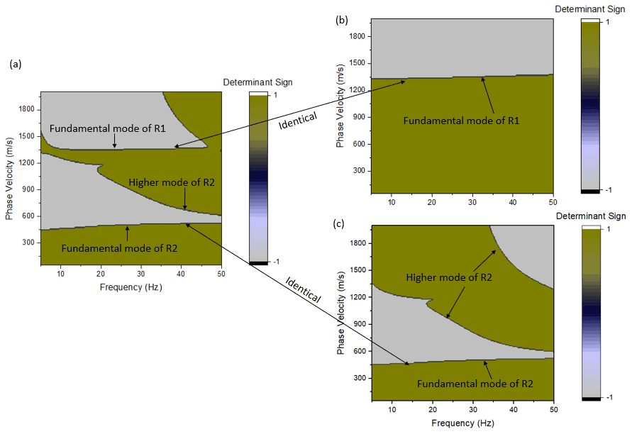
Figure E1 Decomposition of the global stiffness matrix. (a) Dispersion image (a combination of R1 and R2 waves). (b) Dispersion image using the components related only to the P1 and S1 wave velocities. (c) Dispersion image using the components related only to the P2 and S2 wave velocities.

Appendix F: Spectral element matrix components

The components of the S₁ matrix in Eq. (C18) are shown.

${\mathbf{S}}_{\mathrm{1}}(\mathrm{1},\mathrm{1})=-k{p}_{\mathrm{11}}$	${\mathbf{S}}_{\mathrm{1}}(\mathrm{1},\mathrm{2})=-k{p}_{\mathrm{12}}$
${\mathbf{S}}_{\mathrm{1}}(\mathrm{1},\mathrm{3})=-k{p}_{\mathrm{13}}$	${\mathbf{S}}_{\mathrm{1}}(\mathrm{1},\mathrm{4})=k_{\mathrm{S}\mathrm{1}}{q}_{\mathrm{11}}$
${\mathbf{S}}_{\mathrm{1}}(\mathrm{1},\mathrm{5})=k_{\mathrm{S}\mathrm{2}}{q}_{\mathrm{12}}$	${\mathbf{S}}_{\mathrm{1}}(\mathrm{1},\mathrm{6})=k{p}_{\mathrm{11}}\left(-e^{-h{k}_{\mathrm{P}\mathrm{1}}}\right)$
${\mathbf{S}}_{\mathrm{1}}(\mathrm{1},\mathrm{7})=k{p}_{\mathrm{12}}\left(-e^{-h{k}_{\mathrm{P}\mathrm{2}}}\right)$	${\mathbf{S}}_{\mathrm{1}}(\mathrm{1},\mathrm{8})=k{p}_{\mathrm{13}}\left(-e^{-h{k}_{\mathrm{P}\mathrm{3}}}\right)$
${\mathbf{S}}_{\mathrm{1}}(\mathrm{1},\mathrm{9})=k_{\mathrm{S}\mathrm{1}}{q}_{\mathrm{11}}\left(-e^{-h{k}_{\mathrm{S}\mathrm{1}}}\right)$	${\mathbf{S}}_{\mathrm{1}}(\mathrm{1},\mathrm{10})=k_{\mathrm{S}\mathrm{2}}{q}_{\mathrm{12}}\left(-e^{-h{k}_{\mathrm{S}\mathrm{2}}}\right)$

${\mathbf{S}}_{\mathrm{1}}(\mathrm{2},\mathrm{1})=-k_{\mathrm{P}\mathrm{1}}{p}_{\mathrm{11}}$	${\mathbf{S}}_{\mathrm{1}}(\mathrm{2},\mathrm{2})=-k_{\mathrm{P}\mathrm{2}}{p}_{\mathrm{12}}$
${\mathbf{S}}_{\mathrm{1}}(\mathrm{2},\mathrm{3})=-k_{\mathrm{P}\mathrm{3}}{p}_{\mathrm{13}}$	${\mathbf{S}}_{\mathrm{1}}(\mathrm{2},\mathrm{4})=k{q}_{\mathrm{11}}$
${\mathbf{S}}_{\mathrm{1}}(\mathrm{2},\mathrm{5})=k{q}_{\mathrm{12}}$	${\mathbf{S}}_{\mathrm{1}}(\mathrm{2},\mathrm{6})=e^{-h{k}_{\mathrm{P}\mathrm{1}}}{k}_{\mathrm{P}\mathrm{1}}{p}_{\mathrm{11}}$
${\mathbf{S}}_{\mathrm{1}}(\mathrm{2},\mathrm{7})=e^{-h{k}_{\mathrm{P}\mathrm{2}}}{k}_{\mathrm{P}\mathrm{2}}{p}_{\mathrm{12}}$	${\mathbf{S}}_{\mathrm{1}}(\mathrm{2},\mathrm{8})=e^{-h{k}_{\mathrm{P}\mathrm{3}}}{k}_{\mathrm{P}\mathrm{3}}{p}_{\mathrm{13}}$
${\mathbf{S}}_{\mathrm{1}}(\mathrm{2},\mathrm{9})=e^{-h{k}_{\mathrm{S}\mathrm{1}}}k{q}_{\mathrm{11}}$	${\mathbf{S}}_{\mathrm{1}}(\mathrm{2},\mathrm{10})=e^{-h{k}_{\mathrm{S}\mathrm{2}}}k{q}_{\mathrm{12}}$

${\mathbf{S}}_{\mathrm{1}}(\mathrm{3},\mathrm{1})=-k_{\mathrm{P}\mathrm{1}}{p}_{\mathrm{21}}$	${\mathbf{S}}_{\mathrm{1}}(\mathrm{3},\mathrm{2})=-k_{\mathrm{P}\mathrm{2}}{p}_{\mathrm{22}}$
${\mathbf{S}}_{\mathrm{1}}(\mathrm{3},\mathrm{3})=-k_{\mathrm{P}\mathrm{3}}{p}_{\mathrm{23}}$	${\mathbf{S}}_{\mathrm{1}}(\mathrm{3},\mathrm{4})=k(G_{\mathrm{1}}{q}_{\mathrm{11}}+G_{\mathrm{2}}{q}_{\mathrm{21}})$
${\mathbf{S}}_{\mathrm{1}}(\mathrm{3},\mathrm{5})=k(G_{\mathrm{1}}{q}_{\mathrm{12}}+G_{\mathrm{2}}{q}_{\mathrm{22}})$	${\mathbf{S}}_{\mathrm{1}}(\mathrm{3},\mathrm{6})=e^{-h{k}_{\mathrm{P}\mathrm{1}}}{k}_{\mathrm{P}\mathrm{1}}{p}_{\mathrm{21}}$
${\mathbf{S}}_{\mathrm{1}}(\mathrm{3},\mathrm{7})=e^{-h{k}_{\mathrm{P}\mathrm{2}}}{k}_{\mathrm{P}\mathrm{2}}{p}_{\mathrm{22}}$	${\mathbf{S}}_{\mathrm{1}}(\mathrm{3},\mathrm{8})=e^{-h{k}_{\mathrm{P}\mathrm{3}}}{k}_{\mathrm{P}\mathrm{3}}{p}_{\mathrm{23}}$
${\mathbf{S}}_{\mathrm{1}}(\mathrm{3},\mathrm{9})=e^{-h{k}_{\mathrm{S}\mathrm{1}}}k(G_{\mathrm{1}}{q}_{\mathrm{11}}+G_{\mathrm{2}}{q}_{\mathrm{21}})$	${\mathbf{S}}_{\mathrm{1}}(\mathrm{3},\mathrm{10})=e^{-h{k}_{\mathrm{S}\mathrm{2}}}k(G_{\mathrm{1}}{q}_{\mathrm{12}}+G_{\mathrm{2}}{q}_{\mathrm{22}})$

${\mathbf{S}}_{\mathrm{1}}(\mathrm{4},\mathrm{1})=-k_{\mathrm{P}\mathrm{1}}{p}_{\mathrm{21}}$	$S(\mathrm{4},\mathrm{2})=-k_{\mathrm{P}\mathrm{2}}{p}_{\mathrm{22}}$
${\mathbf{S}}_{\mathrm{1}}(\mathrm{4},\mathrm{3})=-k_{\mathrm{P}\mathrm{3}}{p}_{\mathrm{23}}$	${\mathbf{S}}_{\mathrm{1}}(\mathrm{4},\mathrm{4})=k(G_{\mathrm{1}}{q}_{\mathrm{11}}+G_{\mathrm{2}}{q}_{\mathrm{21}})$
${\mathbf{S}}_{\mathrm{1}}(\mathrm{4},\mathrm{5})=k(G_{\mathrm{1}}{q}_{\mathrm{12}}+G_{\mathrm{2}}{q}_{\mathrm{22}})$	${\mathbf{S}}_{\mathrm{1}}(\mathrm{4},\mathrm{6})=e^{-h{k}_{\mathrm{P}\mathrm{1}}}{k}_{\mathrm{P}\mathrm{1}}{p}_{\mathrm{21}}$
${\mathbf{S}}_{\mathrm{1}}(\mathrm{4},\mathrm{7})=e^{-h{k}_{\mathrm{P}\mathrm{2}}}{k}_{\mathrm{P}\mathrm{2}}{p}_{\mathrm{22}}$	${\mathbf{S}}_{\mathrm{1}}(\mathrm{4},\mathrm{8})=e^{-h{k}_{\mathrm{P}\mathrm{3}}}{k}_{\mathrm{P}\mathrm{3}}{p}_{\mathrm{23}}$
${\mathbf{S}}_{\mathrm{1}}(\mathrm{4},\mathrm{9})=e^{-h{k}_{\mathrm{S}\mathrm{1}}}k(G_{\mathrm{1}}{q}_{\mathrm{11}}+G_{\mathrm{2}}{q}_{\mathrm{21}})$	${\mathbf{S}}_{\mathrm{1}}(\mathrm{4},\mathrm{10})=e^{-h{k}_{\mathrm{S}\mathrm{2}}}k(G_{\mathrm{1}}{q}_{\mathrm{12}}+G_{\mathrm{2}}{q}_{\mathrm{22}})$

${\mathbf{S}}_{\mathrm{1}}(\mathrm{5},\mathrm{1})=-k_{\mathrm{P}\mathrm{1}}{p}_{\mathrm{21}}$	$S(\mathrm{5},\mathrm{2})=-k_{\mathrm{P}\mathrm{2}}{p}_{\mathrm{22}}$
${\mathbf{S}}_{\mathrm{1}}(\mathrm{5},\mathrm{3})=-k_{\mathrm{P}\mathrm{3}}{p}_{\mathrm{23}}$	${\mathbf{S}}_{\mathrm{1}}(\mathrm{5},\mathrm{4})=k(G_{\mathrm{1}}{q}_{\mathrm{11}}+G_{\mathrm{2}}{q}_{\mathrm{21}})$
${\mathbf{S}}_{\mathrm{1}}(\mathrm{5},\mathrm{5})=k(G_{\mathrm{1}}{q}_{\mathrm{12}}+G_{\mathrm{2}}{q}_{\mathrm{22}})$	${\mathbf{S}}_{\mathrm{1}}(\mathrm{5},\mathrm{6})=e^{-h{k}_{\mathrm{P}\mathrm{1}}}{k}_{\mathrm{P}\mathrm{1}}{p}_{\mathrm{21}}$
${\mathbf{S}}_{\mathrm{1}}(\mathrm{5},\mathrm{7})=e^{-h{k}_{\mathrm{P}\mathrm{2}}}{k}_{\mathrm{P}\mathrm{2}}{p}_{\mathrm{22}}$	${\mathbf{S}}_{\mathrm{1}}(\mathrm{5},\mathrm{8})=e^{-h{k}_{\mathrm{P}\mathrm{3}}}{k}_{\mathrm{P}\mathrm{3}}{p}_{\mathrm{23}}$
${\mathbf{S}}_{\mathrm{1}}(\mathrm{5},\mathrm{9})=e^{-h{k}_{\mathrm{S}\mathrm{1}}}k(G_{\mathrm{1}}{q}_{\mathrm{11}}+G_{\mathrm{2}}{q}_{\mathrm{21}})$	${\mathbf{S}}_{\mathrm{1}}(\mathrm{5},\mathrm{10})=e^{-h{k}_{\mathrm{S}\mathrm{2}}}k(G_{\mathrm{1}}{q}_{\mathrm{12}}+G_{\mathrm{2}}{q}_{\mathrm{22}})$

${\mathbf{S}}_{\mathrm{1}}(\mathrm{6},\mathrm{1})=-k_{\mathrm{P}\mathrm{1}}{p}_{\mathrm{21}}$	$S(\mathrm{6},\mathrm{2})=-k_{\mathrm{P}\mathrm{2}}{p}_{\mathrm{22}}$
${\mathbf{S}}_{\mathrm{1}}(\mathrm{6},\mathrm{3})=-k_{\mathrm{P}\mathrm{3}}{p}_{\mathrm{23}}$	${\mathbf{S}}_{\mathrm{1}}(\mathrm{6},\mathrm{4})=k(G_{\mathrm{1}}{q}_{\mathrm{11}}+G_{\mathrm{2}}{q}_{\mathrm{21}})$
${\mathbf{S}}_{\mathrm{1}}(\mathrm{6},\mathrm{5})=k(G_{\mathrm{1}}{q}_{\mathrm{12}}+G_{\mathrm{2}}{q}_{\mathrm{22}})$	${\mathbf{S}}_{\mathrm{1}}(\mathrm{6},\mathrm{6})=e^{-h{k}_{\mathrm{P}\mathrm{1}}}{k}_{\mathrm{P}\mathrm{1}}{p}_{\mathrm{21}}$
${\mathbf{S}}_{\mathrm{1}}(\mathrm{6},\mathrm{7})=e^{-h{k}_{\mathrm{P}\mathrm{2}}}{k}_{\mathrm{P}\mathrm{2}}{p}_{\mathrm{22}}$	${\mathbf{S}}_{\mathrm{1}}(\mathrm{6},\mathrm{8})=e^{-h{k}_{\mathrm{P}\mathrm{3}}}{k}_{\mathrm{P}\mathrm{3}}{p}_{\mathrm{23}}$
${\mathbf{S}}_{\mathrm{1}}(\mathrm{6},\mathrm{9})=e^{-h{k}_{\mathrm{S}\mathrm{1}}}k(G_{\mathrm{1}}{q}_{\mathrm{11}}+G_{\mathrm{2}}{q}_{\mathrm{21}})$	${\mathbf{S}}_{\mathrm{1}}(\mathrm{6},\mathrm{10})=e^{-h{k}_{\mathrm{S}\mathrm{2}}}k(G_{\mathrm{1}}{q}_{\mathrm{12}}+G_{\mathrm{2}}{q}_{\mathrm{22}})$

${\mathbf{S}}_{\mathrm{1}}(\mathrm{7},\mathrm{1})=-k_{\mathrm{P}\mathrm{1}}{p}_{\mathrm{21}}$	$S(\mathrm{7},\mathrm{2})=-k_{\mathrm{P}\mathrm{2}}{p}_{\mathrm{22}}$
${\mathbf{S}}_{\mathrm{1}}(\mathrm{7},\mathrm{3})=-k_{\mathrm{P}\mathrm{3}}{p}_{\mathrm{23}}$	${\mathbf{S}}_{\mathrm{1}}(\mathrm{7},\mathrm{4})=k(G_{\mathrm{1}}{q}_{\mathrm{11}}+G_{\mathrm{2}}{q}_{\mathrm{21}})$
${\mathbf{S}}_{\mathrm{1}}(\mathrm{7},\mathrm{5})=k(G_{\mathrm{1}}{q}_{\mathrm{12}}+G_{\mathrm{2}}{q}_{\mathrm{22}})$	${\mathbf{S}}_{\mathrm{1}}(\mathrm{7},\mathrm{6})=e^{-h{k}_{\mathrm{P}\mathrm{1}}}{k}_{\mathrm{P}\mathrm{1}}{p}_{\mathrm{21}}$
${\mathbf{S}}_{\mathrm{1}}(\mathrm{7},\mathrm{7})=e^{-h{k}_{\mathrm{P}\mathrm{2}}}{k}_{\mathrm{P}\mathrm{2}}{p}_{\mathrm{22}}$	${\mathbf{S}}_{\mathrm{1}}(\mathrm{7},\mathrm{8})=e^{-h{k}_{\mathrm{P}\mathrm{3}}}{k}_{\mathrm{P}\mathrm{3}}{p}_{\mathrm{23}}$
${\mathbf{S}}_{\mathrm{1}}(\mathrm{7},\mathrm{9})=e^{-h{k}_{\mathrm{S}\mathrm{1}}}k(G_{\mathrm{1}}{q}_{\mathrm{11}}+G_{\mathrm{2}}{q}_{\mathrm{21}})$	${\mathbf{S}}_{\mathrm{1}}(\mathrm{7},\mathrm{10})=e^{-h{k}_{\mathrm{S}\mathrm{2}}}k(G_{\mathrm{1}}{q}_{\mathrm{12}}+G_{\mathrm{2}}{q}_{\mathrm{22}})$

${\mathbf{S}}_{\mathrm{1}}(\mathrm{8},\mathrm{1})=-k_{\mathrm{P}\mathrm{1}}{p}_{\mathrm{21}}$	$S(\mathrm{8},\mathrm{2})=-k_{\mathrm{P}\mathrm{2}}{p}_{\mathrm{22}}$
${\mathbf{S}}_{\mathrm{1}}(\mathrm{8},\mathrm{3})=-k_{\mathrm{P}\mathrm{3}}{p}_{\mathrm{23}}$	${\mathbf{S}}_{\mathrm{1}}(\mathrm{8},\mathrm{4})=k(G_{\mathrm{1}}{q}_{\mathrm{11}}+G_{\mathrm{2}}{q}_{\mathrm{21}})$
${\mathbf{S}}_{\mathrm{1}}(\mathrm{8},\mathrm{5})=k(G_{\mathrm{1}}{q}_{\mathrm{12}}+G_{\mathrm{2}}{q}_{\mathrm{22}})$	${\mathbf{S}}_{\mathrm{1}}(\mathrm{8},\mathrm{6})=e^{-h{k}_{\mathrm{P}\mathrm{1}}}{k}_{\mathrm{P}\mathrm{1}}{p}_{\mathrm{21}}$
${\mathbf{S}}_{\mathrm{1}}(\mathrm{8},\mathrm{7})=e^{-h{k}_{\mathrm{P}\mathrm{2}}}{k}_{\mathrm{P}\mathrm{2}}{p}_{\mathrm{22}}$	${\mathbf{S}}_{\mathrm{1}}(\mathrm{8},\mathrm{8})=e^{-h{k}_{\mathrm{P}\mathrm{3}}}{k}_{\mathrm{P}\mathrm{3}}{p}_{\mathrm{23}}$
${\mathbf{S}}_{\mathrm{1}}(\mathrm{8},\mathrm{9})=e^{-h{k}_{\mathrm{S}\mathrm{1}}}k(G_{\mathrm{1}}{q}_{\mathrm{11}}+G_{\mathrm{2}}{q}_{\mathrm{21}})$	${\mathbf{S}}_{\mathrm{1}}(\mathrm{8},\mathrm{10})=e^{-h{k}_{\mathrm{S}\mathrm{2}}}k(G_{\mathrm{1}}{q}_{\mathrm{12}}+G_{\mathrm{2}}{q}_{\mathrm{22}})$

${\mathbf{S}}_{\mathrm{1}}(\mathrm{9},\mathrm{1})=-k_{\mathrm{P}\mathrm{1}}{p}_{\mathrm{21}}$	$S(\mathrm{9},\mathrm{2})=-k_{\mathrm{P}\mathrm{2}}{p}_{\mathrm{22}}$
${\mathbf{S}}_{\mathrm{1}}(\mathrm{9},\mathrm{3})=-k_{\mathrm{P}\mathrm{3}}{p}_{\mathrm{23}}$	${\mathbf{S}}_{\mathrm{1}}(\mathrm{9},\mathrm{4})=k(G_{\mathrm{1}}{q}_{\mathrm{11}}+G_{\mathrm{2}}{q}_{\mathrm{21}})$
${\mathbf{S}}_{\mathrm{1}}(\mathrm{9},\mathrm{5})=k(G_{\mathrm{1}}{q}_{\mathrm{12}}+G_{\mathrm{2}}{q}_{\mathrm{22}})$	${\mathbf{S}}_{\mathrm{1}}(\mathrm{9},\mathrm{6})=e^{-h{k}_{\mathrm{P}\mathrm{1}}}{k}_{\mathrm{P}\mathrm{1}}{p}_{\mathrm{21}}$
${\mathbf{S}}_{\mathrm{1}}(\mathrm{9},\mathrm{7})=e^{-h{k}_{\mathrm{P}\mathrm{2}}}{k}_{\mathrm{P}\mathrm{2}}{p}_{\mathrm{22}}$	${\mathbf{S}}_{\mathrm{1}}(\mathrm{9},\mathrm{8})=e^{-h{k}_{\mathrm{P}\mathrm{3}}}{k}_{\mathrm{P}\mathrm{3}}{p}_{\mathrm{23}}$
${\mathbf{S}}_{\mathrm{1}}(\mathrm{9},\mathrm{9})=e^{-h{k}_{\mathrm{S}\mathrm{1}}}k(G_{\mathrm{1}}{q}_{\mathrm{11}}+G_{\mathrm{2}}{q}_{\mathrm{21}})$	${\mathbf{S}}_{\mathrm{1}}(\mathrm{9},\mathrm{10})=e^{-h{k}_{\mathrm{S}\mathrm{2}}}k(G_{\mathrm{1}}{q}_{\mathrm{12}}+G_{\mathrm{2}}{q}_{\mathrm{22}})$

${\mathbf{S}}_{\mathrm{1}}(\mathrm{10},\mathrm{1})=-k_{\mathrm{P}\mathrm{1}}{p}_{\mathrm{21}}$	$S(\mathrm{10},\mathrm{2})=-k_{\mathrm{P}\mathrm{2}}{p}_{\mathrm{22}}$
${\mathbf{S}}_{\mathrm{1}}(\mathrm{10},\mathrm{3})=-k_{\mathrm{P}\mathrm{3}}{p}_{\mathrm{23}}$	${\mathbf{S}}_{\mathrm{1}}(\mathrm{10},\mathrm{4})=k(G_{\mathrm{1}}{q}_{\mathrm{11}}+G_{\mathrm{2}}{q}_{\mathrm{21}})$
${\mathbf{S}}_{\mathrm{1}}(\mathrm{10},\mathrm{5})=k(G_{\mathrm{1}}{q}_{\mathrm{12}}+G_{\mathrm{2}}{q}_{\mathrm{22}})$	${\mathbf{S}}_{\mathrm{1}}(\mathrm{10},\mathrm{6})=e^{-h{k}_{\mathrm{P}\mathrm{1}}}{k}_{\mathrm{P}\mathrm{1}}{p}_{\mathrm{21}}$
${\mathbf{S}}_{\mathrm{1}}(\mathrm{10},\mathrm{7})=e^{-h{k}_{\mathrm{P}\mathrm{2}}}{k}_{\mathrm{P}\mathrm{2}}{p}_{\mathrm{22}}$	${\mathbf{S}}_{\mathrm{1}}(\mathrm{10},\mathrm{8})=e^{-h{k}_{\mathrm{P}\mathrm{3}}}{k}_{\mathrm{P}\mathrm{3}}{p}_{\mathrm{23}}$
${\mathbf{S}}_{\mathrm{1}}(\mathrm{10},\mathrm{9})=e^{-h{k}_{\mathrm{S}\mathrm{1}}}k(G_{\mathrm{1}}{q}_{\mathrm{11}}+G_{\mathrm{2}}{q}_{\mathrm{21}})$	${\mathbf{S}}_{\mathrm{1}}(\mathrm{10},\mathrm{10})=e^{-h{k}_{\mathrm{S}\mathrm{2}}}k(G_{\mathrm{1}}{q}_{\mathrm{12}}+G_{\mathrm{2}}{q}_{\mathrm{22}})$

The components of the S₂ stress matrix in Eq. (C19) are shown.

${\mathbf{S}}_{\mathrm{2}}(\mathrm{1},\mathrm{1})=k{k}_{\mathrm{P}\mathrm{1}}(\mathrm{2}{p}_{\mathrm{11}}{\mathit{\mu }}_{\mathrm{1}}+p_{\mathrm{31}}{\mathit{\mu }}_{\mathrm{13}})$

${\mathbf{S}}_{\mathrm{2}}(\mathrm{1},\mathrm{2})=k{k}_{\mathrm{P}\mathrm{2}}(\mathrm{2}{p}_{\mathrm{12}}{\mathit{\mu }}_{\mathrm{1}}+p_{\mathrm{32}}{\mathit{\mu }}_{\mathrm{13}})$

${\mathbf{S}}_{\mathrm{2}}(\mathrm{1},\mathrm{3})=k{k}_{\mathrm{P}\mathrm{3}}(\mathrm{2}{p}_{\mathrm{13}}{\mathit{\mu }}_{\mathrm{1}}+p_{\mathrm{33}}{\mathit{\mu }}_{\mathrm{13}})$

${\mathbf{S}}_{\mathrm{2}}(\mathrm{1},\mathrm{4})=-\frac{\mathrm{1}}{\mathrm{2}}\left(k^{\mathrm{2}}+k_{\mathrm{S}\mathrm{1}}^{\mathrm{2}}\right)(\mathrm{2}{q}_{\mathrm{11}}{\mathit{\mu }}_{\mathrm{1}}+q_{\mathrm{21}}{\mathit{\mu }}_{\mathrm{13}})$

${\mathbf{S}}_{\mathrm{2}}(\mathrm{1},\mathrm{5})=-\frac{\mathrm{1}}{\mathrm{2}}\left(k^{\mathrm{2}}+k_{\mathrm{S}\mathrm{2}}^{\mathrm{2}}\right)(\mathrm{2}{q}_{\mathrm{12}}{\mathit{\mu }}_{\mathrm{1}}+q_{\mathrm{22}}{\mathit{\mu }}_{\mathrm{13}})$

${\mathbf{S}}_{\mathrm{2}}(\mathrm{1},\mathrm{6})=-e^{-h{k}_{\mathrm{P}\mathrm{1}}}k{k}_{\mathrm{P}\mathrm{1}}(\mathrm{2}{p}_{\mathrm{11}}{\mathit{\mu }}_{\mathrm{1}}+p_{\mathrm{31}}{\mathit{\mu }}_{\mathrm{13}})$

${\mathbf{S}}_{\mathrm{2}}(\mathrm{1},\mathrm{7})=e^{-h{k}_{\mathrm{P}\mathrm{2}}}k{k}_{\mathrm{P}\mathrm{2}}(\mathrm{2}{p}_{\mathrm{12}}{\mathit{\mu }}_{\mathrm{1}}+p_{\mathrm{32}}{\mathit{\mu }}_{\mathrm{13}})$

${\mathbf{S}}_{\mathrm{2}}(\mathrm{1},\mathrm{8})=-e^{-h{k}_{\mathrm{P}\mathrm{3}}}k{k}_{\mathrm{P}\mathrm{3}}(\mathrm{2}{p}_{\mathrm{13}}{\mathit{\mu }}_{\mathrm{1}}+p_{\mathrm{33}}{\mathit{\mu }}_{\mathrm{13}})$

${\mathbf{S}}_{\mathrm{2}}(\mathrm{1},\mathrm{9})=-\frac{\mathrm{1}}{\mathrm{2}}{e}^{-h{k}_{\mathrm{S}\mathrm{1}}}\left(k^{\mathrm{2}}+k_{\mathrm{S}\mathrm{1}}^{\mathrm{2}}\right)(\mathrm{2}{q}_{\mathrm{11}}{\mathit{\mu }}_{\mathrm{1}}+q_{\mathrm{21}}{\mathit{\mu }}_{\mathrm{13}})$

${\mathbf{S}}_{\mathrm{2}}(\mathrm{1},\mathrm{10})=-\frac{\mathrm{1}}{\mathrm{2}}{e}^{-h{k}_{\mathrm{S}\mathrm{2}}}\left(k^{\mathrm{2}}+k_{\mathrm{S}\mathrm{2}}^{\mathrm{2}}\right)(\mathrm{2}{q}_{\mathrm{12}}{\mathit{\mu }}_{\mathrm{1}}+q_{\mathrm{22}}{\mathit{\mu }}_{\mathrm{13}})$

${\mathbf{S}}_{\mathrm{2}}(\mathrm{2},\mathrm{1})=-(p_{\mathrm{11}}{S}_{c\mathrm{1}}+p_{\mathrm{31}}{S}_{c\mathrm{2}})k^{\mathrm{2}}+C_{\mathrm{12}}\left(k_{\mathrm{P}\mathrm{1}}^{\mathrm{2}}-k^{\mathrm{2}}\right)p_{\mathrm{21}}+k_{\mathrm{P}\mathrm{1}}^{\mathrm{2}}\left(p_{\mathrm{11}}\right(S_{c\mathrm{1}}+\mathrm{2}{\mathit{\mu }}_{\mathrm{1}})+p_{\mathrm{31}}(S_{c\mathrm{2}}+{\mathit{\mu }}_{\mathrm{13}}\left)\right)$

${\mathbf{S}}_{\mathrm{2}}(\mathrm{2},\mathrm{2})=-(p_{\mathrm{12}}{S}_{c\mathrm{1}}+p_{\mathrm{32}}{S}_{c\mathrm{2}})k^{\mathrm{2}}+C_{\mathrm{12}}\left(k_{\mathrm{P}\mathrm{2}}^{\mathrm{2}}-k^{\mathrm{2}}\right)p_{\mathrm{22}}+k_{\mathrm{P}\mathrm{2}}^{\mathrm{2}}\left(p_{\mathrm{12}}\right(S_{c\mathrm{1}}+\mathrm{2}{\mathit{\mu }}_{\mathrm{1}})+p_{\mathrm{32}}(S_{c\mathrm{2}}+{\mathit{\mu }}_{\mathrm{13}}\left)\right)$

${\mathbf{S}}_{\mathrm{2}}(\mathrm{2},\mathrm{3})=-(p_{\mathrm{13}}{S}_{c\mathrm{1}}+p_{\mathrm{33}}{S}_{c\mathrm{2}})k^{\mathrm{2}}+C_{\mathrm{12}}\left(k_{\mathrm{P}\mathrm{3}}^{\mathrm{2}}-k^{\mathrm{2}}\right)p_{\mathrm{23}}+k_{\mathrm{P}\mathrm{3}}^{\mathrm{2}}\left(p_{\mathrm{13}}\right(S_{c\mathrm{1}}+\mathrm{2}{\mathit{\mu }}_{\mathrm{1}})+p_{\mathrm{33}}(S_{c\mathrm{2}}+{\mathit{\mu }}_{\mathrm{13}}\left)\right)$

${\mathbf{S}}_{\mathrm{2}}(\mathrm{2},\mathrm{4})=k{k}_{\mathrm{S}\mathrm{1}}(\mathrm{2}{q}_{\mathrm{11}}{\mathit{\mu }}_{\mathrm{1}}+q_{\mathrm{21}}{\mathit{\mu }}_{\mathrm{13}})$

${\mathbf{S}}_{\mathrm{2}}(\mathrm{2},\mathrm{5})=k{k}_{\mathrm{S}\mathrm{2}}(\mathrm{2}{q}_{\mathrm{12}}{\mathit{\mu }}_{\mathrm{1}}+q_{\mathrm{22}}{\mathit{\mu }}_{\mathrm{13}})$

${\mathbf{S}}_{\mathrm{2}}(\mathrm{2},\mathrm{6})=e^{-h{k}_{\mathrm{P}\mathrm{1}}}\left(-(p_{\mathrm{11}}{S}_{c\mathrm{1}}+p_{\mathrm{31}}{S}_{c\mathrm{2}})k^{\mathrm{2}}+C_{\mathrm{12}}\left(k_{\mathrm{P}\mathrm{1}}^{\mathrm{2}}-k^{\mathrm{2}}\right)p_{\mathrm{21}}+k_{\mathrm{P}\mathrm{1}}^{\mathrm{2}}\left(p_{\mathrm{11}}\right(S_{c\mathrm{1}}+\mathrm{2}{\mathit{\mu }}_{\mathrm{1}})+p_{\mathrm{31}}(S_{c\mathrm{2}}+{\mathit{\mu }}_{\mathrm{13}}\left)\right)\right)$

${\mathbf{S}}_{\mathrm{2}}(\mathrm{2},\mathrm{7})=e^{-h{k}_{\mathrm{P}\mathrm{2}}}\left(-(p_{\mathrm{12}}{S}_{c\mathrm{1}}+p_{\mathrm{32}}{S}_{c\mathrm{2}})k^{\mathrm{2}}+C_{\mathrm{12}}\left(k_{\mathrm{P}\mathrm{2}}^{\mathrm{2}}-k^{\mathrm{2}}\right)p_{\mathrm{22}}+k_{\mathrm{P}\mathrm{2}}^{\mathrm{2}}\left(p_{\mathrm{12}}\right(S_{c\mathrm{1}}+\mathrm{2}{\mathit{\mu }}_{\mathrm{1}})+p_{\mathrm{32}}(S_{c\mathrm{2}}+{\mathit{\mu }}_{\mathrm{13}}\left)\right)\right)$

${\mathbf{S}}_{\mathrm{2}}(\mathrm{2},\mathrm{8})=e^{-h{k}_{\mathrm{P}\mathrm{3}}}\left(-(p_{\mathrm{13}}{S}_{c\mathrm{1}}+p_{\mathrm{33}}{S}_{c\mathrm{2}})k^{\mathrm{2}}+C_{\mathrm{12}}\left(k_{\mathrm{P}\mathrm{3}}^{\mathrm{2}}-k^{\mathrm{2}}\right)p_{\mathrm{23}}+k_{\mathrm{P}\mathrm{3}}^{\mathrm{2}}\left(p_{\mathrm{13}}\right(S_{c\mathrm{1}}+\mathrm{2}{\mathit{\mu }}_{\mathrm{1}})+p_{\mathrm{33}}(S_{c\mathrm{2}}+{\mathit{\mu }}_{\mathrm{13}}\left)\right)\right)$

${\mathbf{S}}_{\mathrm{2}}(\mathrm{2},\mathrm{9})=e^{-h{k}_{\mathrm{S}\mathrm{1}}}k{k}_{\mathrm{S}\mathrm{1}}(\mathrm{2}{q}_{\mathrm{11}}{\mathit{\mu }}_{\mathrm{1}}+q_{\mathrm{21}}{\mathit{\mu }}_{\mathrm{13}})$

${\mathbf{S}}_{\mathrm{2}}(\mathrm{2},\mathrm{10})=e^{-h{k}_{\mathrm{S}\mathrm{2}}}k{k}_{\mathrm{S}\mathrm{2}}(\mathrm{2}{q}_{\mathrm{12}}{\mathit{\mu }}_{\mathrm{1}}+q_{\mathrm{22}}{\mathit{\mu }}_{\mathrm{13}})$

${\mathbf{S}}_{\mathrm{2}}(\mathrm{3},\mathrm{1})=(k_{\mathrm{P}\mathrm{1}}-k)(k+k_{\mathrm{P}\mathrm{1}})(C_{\mathrm{12}}{p}_{\mathrm{11}}+k_{\mathrm{2}}{p}_{\mathrm{21}}+C_{\mathrm{23}}{p}_{\mathrm{31}})$

${\mathbf{S}}_{\mathrm{2}}(\mathrm{3},\mathrm{2})=-(k-k_{\mathrm{P}\mathrm{2}})(k+k_{\mathrm{P}\mathrm{2}})(C_{\mathrm{12}}{p}_{\mathrm{12}}+k_{\mathrm{2}}{p}_{\mathrm{22}}+C_{\mathrm{23}}{p}_{\mathrm{32}})$

${\mathbf{S}}_{\mathrm{2}}(\mathrm{3},\mathrm{3})=-(k-k_{\mathrm{P}\mathrm{3}})(k+k_{\mathrm{P}\mathrm{3}})(C_{\mathrm{12}}{p}_{\mathrm{13}}+k_{\mathrm{2}}{p}_{\mathrm{23}}+C_{\mathrm{23}}{p}_{\mathrm{33}})$

${\mathbf{S}}_{\mathrm{2}}(\mathrm{3},\mathrm{4})=\mathrm{0}$

${\mathbf{S}}_{\mathrm{2}}(\mathrm{3},\mathrm{5})=\mathrm{0}$

${\mathbf{S}}_{\mathrm{2}}(\mathrm{3},\mathrm{6})=e^{-h{k}_{\mathrm{P}\mathrm{1}}}(k_{\mathrm{P}\mathrm{1}}-k)(k+k_{\mathrm{P}\mathrm{1}})(C_{\mathrm{12}}{p}_{\mathrm{11}}+k_{\mathrm{2}}{p}_{\mathrm{21}}+C_{\mathrm{23}}{p}_{\mathrm{31}})$

${\mathbf{S}}_{\mathrm{2}}(\mathrm{3},\mathrm{7})=e^{-h{k}_{\mathrm{P}\mathrm{2}}}(k_{\mathrm{P}\mathrm{2}}-k)(k+k_{\mathrm{P}\mathrm{2}})(C_{\mathrm{12}}{p}_{\mathrm{12}}+k_{\mathrm{2}}{p}_{\mathrm{22}}+C_{\mathrm{23}}{p}_{\mathrm{32}})$

${\mathbf{S}}_{\mathrm{2}}(\mathrm{3},\mathrm{8})=e^{-h{k}_{\mathrm{P}\mathrm{3}}}(k_{\mathrm{P}\mathrm{3}}-k)(k+k_{\mathrm{P}\mathrm{3}})(C_{\mathrm{12}}{p}_{\mathrm{13}}+k_{\mathrm{2}}{p}_{\mathrm{23}}+C_{\mathrm{23}}{p}_{\mathrm{33}})$

${\mathbf{S}}_{\mathrm{2}}(\mathrm{3},\mathrm{9})=\mathrm{0}$

${\mathbf{S}}_{\mathrm{2}}(\mathrm{3},\mathrm{10})=\mathrm{0}$

${\mathbf{S}}_{\mathrm{2}}(\mathrm{4},\mathrm{1})=k{k}_{\mathrm{P}\mathrm{1}}(p_{\mathrm{11}}{\mathit{\mu }}_{\mathrm{13}}+\mathrm{2}{p}_{\mathrm{31}}{\mathit{\mu }}_{\mathrm{3}})$

${\mathbf{S}}_{\mathrm{2}}(\mathrm{4},\mathrm{2})=k{k}_{\mathrm{P}\mathrm{2}}(p_{\mathrm{12}}{\mathit{\mu }}_{\mathrm{13}}+\mathrm{2}{p}_{\mathrm{32}}{\mathit{\mu }}_{\mathrm{3}})$

${\mathbf{S}}_{\mathrm{2}}(\mathrm{4},\mathrm{3})=k{k}_{\mathrm{P}\mathrm{3}}(p_{\mathrm{13}}{\mathit{\mu }}_{\mathrm{13}}+\mathrm{2}{p}_{\mathrm{33}}{\mathit{\mu }}_{\mathrm{3}})$

${\mathbf{S}}_{\mathrm{2}}(\mathrm{4},\mathrm{4})=-\frac{\mathrm{1}}{\mathrm{2}}\left(k^{\mathrm{2}}+k_{\mathrm{S}\mathrm{1}}^{\mathrm{2}}\right)(q_{\mathrm{11}}{\mathit{\mu }}_{\mathrm{13}}+\mathrm{2}{q}_{\mathrm{21}}{\mathit{\mu }}_{\mathrm{3}})$

${\mathbf{S}}_{\mathrm{2}}(\mathrm{4},\mathrm{5})=-\frac{\mathrm{1}}{\mathrm{2}}\left(k^{\mathrm{2}}+k_{\mathrm{S}\mathrm{2}}^{\mathrm{2}}\right)(q_{\mathrm{12}}{\mathit{\mu }}_{\mathrm{13}}+\mathrm{2}{q}_{\mathrm{22}}{\mathit{\mu }}_{\mathrm{3}})$

${\mathbf{S}}_{\mathrm{2}}(\mathrm{4},\mathrm{6})=-e^{-h{k}_{\mathrm{P}\mathrm{1}}}k{k}_{\mathrm{P}\mathrm{1}}(p_{\mathrm{11}}{\mathit{\mu }}_{\mathrm{13}}+\mathrm{2}{p}_{\mathrm{31}}{\mathit{\mu }}_{\mathrm{3}})$

${\mathbf{S}}_{\mathrm{2}}(\mathrm{4},\mathrm{7})=-e^{-h{k}_{\mathrm{P}\mathrm{2}}}k{k}_{\mathrm{P}\mathrm{2}}(p_{\mathrm{12}}{\mathit{\mu }}_{\mathrm{13}}+\mathrm{2}{p}_{\mathrm{32}}{\mathit{\mu }}_{\mathrm{3}})$

${\mathbf{S}}_{\mathrm{2}}(\mathrm{4},\mathrm{8})=-e^{-h{k}_{\mathrm{P}\mathrm{3}}}k{k}_{\mathrm{P}\mathrm{3}}(p_{\mathrm{13}}{\mathit{\mu }}_{\mathrm{13}}+\mathrm{2}{P}_{\mathrm{33}}{\mathit{\mu }}_{\mathrm{3}})$

${\mathbf{S}}_{\mathrm{2}}(\mathrm{4},\mathrm{9})=-\frac{\mathrm{1}}{\mathrm{2}}{e}^{-h{k}_{\mathrm{S}\mathrm{1}}}\left(k^{\mathrm{2}}+k_{\mathrm{S}\mathrm{1}}^{\mathrm{2}}\right)(q_{\mathrm{11}}{\mathit{\mu }}_{\mathrm{13}}+\mathrm{2}{q}_{\mathrm{21}}{\mathit{\mu }}_{\mathrm{3}})$

${\mathbf{S}}_{\mathrm{2}}(\mathrm{4},\mathrm{10})=-\frac{\mathrm{1}}{\mathrm{2}}{e}^{-h{k}_{\mathrm{S}\mathrm{2}}}\left(k^{\mathrm{2}}+k_{\mathrm{S}\mathrm{2}}^{\mathrm{2}}\right)(q_{\mathrm{12}}{\mathit{\mu }}_{\mathrm{13}}+\mathrm{2}{q}_{\mathrm{22}}{\mathit{\mu }}_{\mathrm{3}})$

${\mathbf{S}}_{\mathrm{2}}(\mathrm{5},\mathrm{1})=-(p_{\mathrm{31}}{S}_{c\mathrm{3}}+p_{\mathrm{11}}{S}_{c\mathrm{4}})k^{\mathrm{2}}+C_{\mathrm{23}}\left(k_{\mathrm{P}\mathrm{1}}^{\mathrm{2}}-k^{\mathrm{2}}\right)p_{\mathrm{21}}+k_{\mathrm{P}\mathrm{1}}^{\mathrm{2}}\left(p_{\mathrm{11}}\right(S_{c\mathrm{4}}+{\mathit{\mu }}_{\mathrm{13}})+p_{\mathrm{31}}(S_{c\mathrm{3}}+\mathrm{2}{\mathit{\mu }}_{\mathrm{3}}\left)\right)$

${\mathbf{S}}_{\mathrm{2}}(\mathrm{5},\mathrm{2})=-(p_{\mathrm{32}}{S}_{c\mathrm{3}}+p_{\mathrm{12}}{S}_{c\mathrm{4}})k^{\mathrm{2}}+C_{\mathrm{23}}\left(k_{\mathrm{P}\mathrm{2}}^{\mathrm{2}}-k^{\mathrm{2}}\right)p_{\mathrm{22}}+k_{\mathrm{P}\mathrm{2}}^{\mathrm{2}}\left(p_{\mathrm{12}}\right(S_{c\mathrm{4}}+{\mathit{\mu }}_{\mathrm{13}})+p_{\mathrm{32}}(S_{c\mathrm{3}}+\mathrm{2}{\mathit{\mu }}_{\mathrm{3}}\left)\right)$

${\mathbf{S}}_{\mathrm{2}}(\mathrm{5},\mathrm{3})=-(p_{\mathrm{33}}{S}_{c\mathrm{3}}+p_{\mathrm{13}}{S}_{c\mathrm{4}})k^{\mathrm{2}}+C_{\mathrm{23}}\left(k_{\mathrm{P}\mathrm{3}}^{\mathrm{2}}-k^{\mathrm{2}}\right)p_{\mathrm{23}}+k_{\mathrm{P}\mathrm{3}}^{\mathrm{2}}\left(p_{\mathrm{13}}\right(S_{c\mathrm{4}}+{\mathit{\mu }}_{\mathrm{13}})+p_{\mathrm{33}}(S_{c\mathrm{3}}+\mathrm{2}{\mathit{\mu }}_{\mathrm{3}}\left)\right)$

${\mathbf{S}}_{\mathrm{2}}(\mathrm{5},\mathrm{4})=-k{k}_{\mathrm{S}\mathrm{1}}(q_{\mathrm{11}}{\mathit{\mu }}_{\mathrm{13}}+\mathrm{2}{q}_{\mathrm{21}}{\mathit{\mu }}_{\mathrm{3}})$

${\mathbf{S}}_{\mathrm{2}}(\mathrm{5},\mathrm{5})=-k{k}_{\mathrm{S}\mathrm{2}}(q_{\mathrm{12}}{\mathit{\mu }}_{\mathrm{13}}+\mathrm{2}{q}_{\mathrm{22}}{\mathit{\mu }}_{\mathrm{3}})$

${\mathbf{S}}_{\mathrm{2}}(\mathrm{5},\mathrm{6})=e^{-h{k}_{\mathrm{P}\mathrm{1}}}\left(-(p_{\mathrm{31}}{S}_{c\mathrm{3}}+p_{\mathrm{11}}{S}_{c\mathrm{4}})k^{\mathrm{2}}+C_{\mathrm{23}}\left(k_{\mathrm{P}\mathrm{1}}^{\mathrm{2}}-k^{\mathrm{2}}\right)p_{\mathrm{21}}+k_{\mathrm{P}\mathrm{1}}^{\mathrm{2}}\left(p_{\mathrm{11}}\right(S_{c\mathrm{4}}+{\mathit{\mu }}_{\mathrm{13}})+p_{\mathrm{31}}(S_{c\mathrm{3}}+\mathrm{2}{\mathit{\mu }}_{\mathrm{3}}\left)\right)\right)$

${\mathbf{S}}_{\mathrm{2}}(\mathrm{5},\mathrm{7})=e^{-h{k}_{\mathrm{P}\mathrm{2}}}\left(-(p_{\mathrm{32}}{S}_{c\mathrm{3}}+p_{\mathrm{12}}{S}_{c\mathrm{4}})k^{\mathrm{2}}+C_{\mathrm{23}}\left(k_{\mathrm{P}\mathrm{2}}^{\mathrm{2}}-k^{\mathrm{2}}\right)p_{\mathrm{22}}+k_{\mathrm{P}\mathrm{2}}^{\mathrm{2}}\left(p_{\mathrm{12}}\right(S_{c\mathrm{4}}+{\mathit{\mu }}_{\mathrm{13}})+p_{\mathrm{32}}(S_{c\mathrm{3}}+\mathrm{2}{\mathit{\mu }}_{\mathrm{3}}\left)\right)\right)$

${\mathbf{S}}_{\mathrm{2}}(\mathrm{5},\mathrm{8})=e^{-h{k}_{\mathrm{P}\mathrm{3}}}\left(-(p_{\mathrm{33}}{S}_{c\mathrm{3}}+p_{\mathrm{13}}{S}_{c\mathrm{4}})k^{\mathrm{2}}+C_{\mathrm{23}}\left(k_{\mathrm{P}\mathrm{3}}^{\mathrm{2}}-k^{\mathrm{2}}\right)p_{\mathrm{23}}+k_{\mathrm{P}\mathrm{3}}^{\mathrm{2}}\left(p_{\mathrm{13}}\right(S_{c\mathrm{4}}+{\mathit{\mu }}_{\mathrm{13}})+p_{\mathrm{33}}(S_{c\mathrm{3}}+\mathrm{2}{\mathit{\mu }}_{\mathrm{3}}\left)\right)\right)$

${\mathbf{S}}_{\mathrm{2}}(\mathrm{5},\mathrm{9})=e^{-h{k}_{\mathrm{S}\mathrm{1}}}k{k}_{\mathrm{S}\mathrm{1}}(q_{\mathrm{11}}{\mathit{\mu }}_{\mathrm{13}}+\mathrm{2}{q}_{\mathrm{21}}{\mathit{\mu }}_{\mathrm{3}})$

${\mathbf{S}}_{\mathrm{2}}(\mathrm{5},\mathrm{10})=e^{-h{k}_{\mathrm{S}\mathrm{2}}}k{k}_{\mathrm{S}\mathrm{2}}(q_{\mathrm{12}}{\mathit{\mu }}_{\mathrm{13}}+\mathrm{2}{q}_{\mathrm{22}}{\mathit{\mu }}_{\mathrm{3}})$

${\mathbf{S}}_{\mathrm{2}}(\mathrm{6},\mathrm{1})=k{k}_{\mathrm{P}\mathrm{1}}{e}^{-h{k}_{\mathrm{P}\mathrm{1}}}(\mathrm{2}{\mathit{\mu }}_{\mathrm{1}}{p}_{\mathrm{11}}+{\mathit{\mu }}_{\mathrm{13}}{p}_{\mathrm{31}})$

${\mathbf{S}}_{\mathrm{2}}(\mathrm{6},\mathrm{2})=k{k}_{\mathrm{P}\mathrm{2}}{e}^{-h{k}_{\mathrm{P}\mathrm{2}}}(\mathrm{2}{\mathit{\mu }}_{\mathrm{1}}{p}_{\mathrm{12}}+{\mathit{\mu }}_{\mathrm{13}}{p}_{\mathrm{32}})$

${\mathbf{S}}_{\mathrm{2}}(\mathrm{6},\mathrm{3})=k{k}_{\mathrm{P}\mathrm{3}}{e}^{-h{k}_{\mathrm{P}\mathrm{3}}}(\mathrm{2}{\mathit{\mu }}_{\mathrm{1}}{p}_{\mathrm{13}}+{\mathit{\mu }}_{\mathrm{13}}{p}_{\mathrm{33}})$

${\mathbf{S}}_{\mathrm{2}}(\mathrm{6},\mathrm{4})=-\frac{\mathrm{1}}{\mathrm{2}}{e}^{-h{k}_{\mathrm{S}\mathrm{1}}}\left(k^{\mathrm{2}}+k_{\mathrm{S}\mathrm{1}}^{\mathrm{2}}\right)(\mathrm{2}{\mathit{\mu }}_{\mathrm{1}}{q}_{\mathrm{11}}+{\mathit{\mu }}_{\mathrm{13}}{q}_{\mathrm{21}})$

${\mathbf{S}}_{\mathrm{2}}(\mathrm{6},\mathrm{5})=-\frac{\mathrm{1}}{\mathrm{2}}{e}^{-h{k}_{\mathrm{S}\mathrm{2}}}\left(k^{\mathrm{2}}+k_{\mathrm{S}\mathrm{2}}^{\mathrm{2}}\right)(\mathrm{2}{\mathit{\mu }}_{\mathrm{1}}{q}_{\mathrm{12}}+{\mathit{\mu }}_{\mathrm{13}}{q}_{\mathrm{22}})$

${\mathbf{S}}_{\mathrm{2}}(\mathrm{6},\mathrm{6})=-k{k}_{\mathrm{P}\mathrm{1}}(\mathrm{2}{\mathit{\mu }}_{\mathrm{1}}{p}_{\mathrm{11}}+{\mathit{\mu }}_{\mathrm{13}}{p}_{\mathrm{31}})$

${\mathbf{S}}_{\mathrm{2}}(\mathrm{6},\mathrm{7})=-k{k}_{\mathrm{P}\mathrm{2}}(\mathrm{2}{\mathit{\mu }}_{\mathrm{1}}{p}_{\mathrm{12}}+{\mathit{\mu }}_{\mathrm{13}}{p}_{\mathrm{32}})$

${\mathbf{S}}_{\mathrm{2}}(\mathrm{6},\mathrm{8})=-k{k}_{\mathrm{P}\mathrm{3}}(\mathrm{2}{\mathit{\mu }}_{\mathrm{1}}{p}_{\mathrm{13}}+{\mathit{\mu }}_{\mathrm{13}}{p}_{\mathrm{33}})$

${\mathbf{S}}_{\mathrm{2}}(\mathrm{6},\mathrm{9})=-\frac{\mathrm{1}}{\mathrm{2}}\left(k^{\mathrm{2}}+k_{\mathrm{S}\mathrm{1}}^{\mathrm{2}}\right)(\mathrm{2}{\mathit{\mu }}_{\mathrm{1}}{q}_{\mathrm{11}}+{\mathit{\mu }}_{\mathrm{13}}{q}_{\mathrm{21}})$

${\mathbf{S}}_{\mathrm{2}}(\mathrm{6},\mathrm{10})=-\frac{\mathrm{1}}{\mathrm{2}}\left(k^{\mathrm{2}}+k_{\mathrm{S}\mathrm{2}}^{\mathrm{2}}\right)(\mathrm{2}{\mathit{\mu }}_{\mathrm{1}}{q}_{\mathrm{12}}+{\mathit{\mu }}_{\mathrm{13}}{q}_{\mathrm{22}})$

${\mathbf{S}}_{\mathrm{2}}(\mathrm{7},\mathrm{1})=e^{-h{k}_{\mathrm{P}\mathrm{1}}}\left(-(p_{\mathrm{11}}{S}_{c\mathrm{1}}+p_{\mathrm{31}}{S}_{c\mathrm{2}})k^{\mathrm{2}}+C_{\mathrm{12}}\left(k_{\mathrm{P}\mathrm{1}}^{\mathrm{2}}-k^{\mathrm{2}}\right)p_{\mathrm{21}}+k_{\mathrm{P}\mathrm{1}}^{\mathrm{2}}\left(p_{\mathrm{11}}\right(S_{c\mathrm{1}}+\mathrm{2}{\mathit{\mu }}_{\mathrm{1}})+p_{\mathrm{31}}(S_{c\mathrm{2}}+{\mathit{\mu }}_{\mathrm{13}}\left)\right)\right)$

${\mathbf{S}}_{\mathrm{2}}(\mathrm{7},\mathrm{2})=e^{-h{k}_{\mathrm{P}\mathrm{2}}}\left(-(p_{\mathrm{12}}{S}_{c\mathrm{1}}+p_{\mathrm{32}}{S}_{c\mathrm{2}})k^{\mathrm{2}}+C_{\mathrm{12}}\left(k_{\mathrm{P}\mathrm{2}}^{\mathrm{2}}-k^{\mathrm{2}}\right)p_{\mathrm{22}}+k_{\mathrm{P}\mathrm{2}}^{\mathrm{2}}\left(p_{\mathrm{12}}\right(S_{c\mathrm{1}}+\mathrm{2}{\mathit{\mu }}_{\mathrm{1}})+p_{\mathrm{32}}(S_{c\mathrm{2}}+{\mathit{\mu }}_{\mathrm{13}}\left)\right)\right)$

${\mathbf{S}}_{\mathrm{2}}(\mathrm{7},\mathrm{3})=e^{-h{k}_{\mathrm{P}\mathrm{3}}}\left(-(p_{\mathrm{13}}{S}_{c\mathrm{1}}+p_{\mathrm{33}}{S}_{c\mathrm{2}})k^{\mathrm{2}}+C_{\mathrm{12}}\left(k_{\mathrm{P}\mathrm{3}}^{\mathrm{2}}-k^{\mathrm{2}}\right)p_{\mathrm{23}}+k_{\mathrm{P}\mathrm{3}}^{\mathrm{2}}\left(p_{\mathrm{13}}\right(S_{c\mathrm{1}}+\mathrm{2}{\mathit{\mu }}_{\mathrm{1}})+p_{\mathrm{33}}(S_{c\mathrm{2}}+{\mathit{\mu }}_{\mathrm{13}}\left)\right)\right)$

${\mathbf{S}}_{\mathrm{2}}(\mathrm{7},\mathrm{4})=-e^{-h{k}_{\mathrm{S}\mathrm{1}}}k{k}_{\mathrm{S}\mathrm{1}}(\mathrm{2}{q}_{\mathrm{11}}{\mathit{\mu }}_{\mathrm{1}}+q_{\mathrm{21}}{\mathit{\mu }}_{\mathrm{13}})$

${\mathbf{S}}_{\mathrm{2}}(\mathrm{7},\mathrm{5})=-e^{-h{k}_{\mathrm{S}\mathrm{2}}}k{k}_{\mathrm{S}\mathrm{2}}(\mathrm{2}{q}_{\mathrm{12}}{\mathit{\mu }}_{\mathrm{1}}+q_{\mathrm{22}}{\mathit{\mu }}_{\mathrm{13}})$

${\mathbf{S}}_{\mathrm{2}}(\mathrm{7},\mathrm{6})=-(p_{\mathrm{11}}{S}_{c\mathrm{1}}+p_{\mathrm{31}}{S}_{c\mathrm{2}})k^{\mathrm{2}}+C_{\mathrm{12}}\left(k_{\mathrm{P}\mathrm{1}}^{\mathrm{2}}-k^{\mathrm{2}}\right)p_{\mathrm{21}}+k_{\mathrm{P}\mathrm{1}}^{\mathrm{2}}\left(p_{\mathrm{11}}\right(S_{c\mathrm{1}}+\mathrm{2}{\mathit{\mu }}_{\mathrm{1}})+p_{\mathrm{31}}(S_{c\mathrm{2}}+{\mathit{\mu }}_{\mathrm{13}}\left)\right)$

${\mathbf{S}}_{\mathrm{2}}(\mathrm{7},\mathrm{7})=-(p_{\mathrm{12}}{S}_{c\mathrm{1}}+p_{\mathrm{32}}{S}_{c\mathrm{2}})k^{\mathrm{2}}+C_{\mathrm{12}}\left(k_{\mathrm{P}\mathrm{2}}^{\mathrm{2}}-k^{\mathrm{2}}\right)p_{\mathrm{22}}+k_{\mathrm{P}\mathrm{2}}^{\mathrm{2}}\left(p_{\mathrm{12}}\right(S_{c\mathrm{1}}+\mathrm{2}{\mathit{\mu }}_{\mathrm{1}})+p_{\mathrm{32}}(S_{c\mathrm{2}}+{\mathit{\mu }}_{\mathrm{13}}\left)\right)$

${\mathbf{S}}_{\mathrm{2}}(\mathrm{7},\mathrm{8})=-(p_{\mathrm{13}}{S}_{c\mathrm{1}}+p_{\mathrm{33}}{S}_{c\mathrm{2}})k^{\mathrm{2}}+C_{\mathrm{12}}\left(k_{\mathrm{P}\mathrm{3}}^{\mathrm{2}}-k^{\mathrm{2}}\right)p_{\mathrm{23}}+k_{\mathrm{P}\mathrm{3}}^{\mathrm{2}}\left(p_{\mathrm{13}}\right(S_{c\mathrm{1}}+\mathrm{2}{\mathit{\mu }}_{\mathrm{1}})+p_{\mathrm{33}}(S_{c\mathrm{2}}+{\mathit{\mu }}_{\mathrm{13}}\left)\right)$

${\mathbf{S}}_{\mathrm{2}}(\mathrm{7},\mathrm{9})=k{k}_{\mathrm{S}\mathrm{1}}(\mathrm{2}{q}_{\mathrm{11}}{\mathit{\mu }}_{\mathrm{1}}+q_{\mathrm{21}}{\mathit{\mu }}_{\mathrm{13}})$

${\mathbf{S}}_{\mathrm{2}}(\mathrm{7},\mathrm{10})=k{k}_{\mathrm{S}\mathrm{2}}(\mathrm{2}{q}_{\mathrm{12}}{\mathit{\mu }}_{\mathrm{1}}+q_{\mathrm{22}}{\mathit{\mu }}_{\mathrm{13}})$

${\mathbf{S}}_{\mathrm{2}}(\mathrm{8},\mathrm{1})=e^{-h{k}_{\mathrm{P}\mathrm{1}}}(k_{\mathrm{P}\mathrm{1}}-k)(k+k_{\mathrm{P}\mathrm{1}})(C_{\mathrm{12}}{p}_{\mathrm{11}}+k_{\mathrm{2}}{p}_{\mathrm{21}}+C_{\mathrm{23}}{p}_{\mathrm{31}})$

${\mathbf{S}}_{\mathrm{2}}(\mathrm{8},\mathrm{2})=e^{-h{k}_{\mathrm{P}\mathrm{2}}}(k_{\mathrm{P}\mathrm{2}}-k)(k+k_{\mathrm{P}\mathrm{2}})(C_{\mathrm{12}}{p}_{\mathrm{12}}+k_{\mathrm{2}}{p}_{\mathrm{22}}+C_{\mathrm{23}}{p}_{\mathrm{32}})$

${\mathbf{S}}_{\mathrm{2}}(\mathrm{8},\mathrm{3})=e^{-h{k}_{\mathrm{P}\mathrm{3}}}(k_{\mathrm{P}\mathrm{3}}-k)(k+k_{\mathrm{P}\mathrm{3}})(C_{\mathrm{12}}{p}_{\mathrm{13}}+k_{\mathrm{2}}{p}_{\mathrm{23}}+C_{\mathrm{23}}{P}_{\mathrm{33}})$

${\mathbf{S}}_{\mathrm{2}}(\mathrm{8},\mathrm{4})=\mathrm{0}$

${\mathbf{S}}_{\mathrm{2}}(\mathrm{8},\mathrm{5})=\mathrm{0}$

${\mathbf{S}}_{\mathrm{2}}(\mathrm{8},\mathrm{6})=(k_{\mathrm{P}\mathrm{1}}-k)(k+k_{\mathrm{P}\mathrm{1}})(C_{\mathrm{12}}{p}_{\mathrm{11}}+k_{\mathrm{2}}{p}_{\mathrm{21}}+C_{\mathrm{23}}{p}_{\mathrm{31}})$

${\mathbf{S}}_{\mathrm{2}}(\mathrm{8},\mathrm{7})=(k_{\mathrm{P}\mathrm{2}}-k)(k+k_{\mathrm{P}\mathrm{2}})(C_{\mathrm{12}}{p}_{\mathrm{12}}+k_{\mathrm{2}}{p}_{\mathrm{22}}+C_{\mathrm{23}}{p}_{\mathrm{32}})$

${\mathbf{S}}_{\mathrm{2}}(\mathrm{8},\mathrm{8})=(k_{\mathrm{P}\mathrm{3}}-k)(k+k_{\mathrm{P}\mathrm{3}})(C_{\mathrm{12}}{p}_{\mathrm{13}}+k_{\mathrm{2}}{p}_{\mathrm{23}}+C_{\mathrm{23}}{P}_{\mathrm{33}})$

${\mathbf{S}}_{\mathrm{2}}(\mathrm{8},\mathrm{9})=\mathrm{0}$

${\mathbf{S}}_{\mathrm{2}}(\mathrm{8},\mathrm{10})=\mathrm{0}$

${\mathbf{S}}_{\mathrm{2}}(\mathrm{9},\mathrm{1})=k{k}_{\mathrm{P}\mathrm{1}}{e}^{-h{k}_{\mathrm{P}\mathrm{1}}}({\mathit{\mu }}_{\mathrm{13}}{p}_{\mathrm{11}}+\mathrm{2}{\mathit{\mu }}_{\mathrm{3}}{p}_{\mathrm{31}})$

${\mathbf{S}}_{\mathrm{2}}(\mathrm{9},\mathrm{2})=k{k}_{\mathrm{P}\mathrm{2}}{e}^{-h{k}_{\mathrm{P}\mathrm{2}}}({\mathit{\mu }}_{\mathrm{13}}{p}_{\mathrm{12}}+\mathrm{2}{\mathit{\mu }}_{\mathrm{3}}{p}_{\mathrm{32}})$

${\mathbf{S}}_{\mathrm{2}}(\mathrm{9},\mathrm{3})=k{k}_{\mathrm{P}\mathrm{3}}{e}^{-h{k}_{\mathrm{P}\mathrm{3}}}({\mathit{\mu }}_{\mathrm{13}}{p}_{\mathrm{13}}+\mathrm{2}{\mathit{\mu }}_{\mathrm{3}}{p}_{\mathrm{33}})$

${\mathbf{S}}_{\mathrm{2}}(\mathrm{9},\mathrm{4})=-\frac{\mathrm{1}}{\mathrm{2}}{e}^{-h{k}_{\mathrm{S}\mathrm{1}}}\left(k^{\mathrm{2}}+k_{\mathrm{S}\mathrm{1}}^{\mathrm{2}}\right)({\mathit{\mu }}_{\mathrm{13}}{q}_{\mathrm{11}}+\mathrm{2}{\mathit{\mu }}_{\mathrm{3}}{q}_{\mathrm{21}})$

${\mathbf{S}}_{\mathrm{2}}(\mathrm{9},\mathrm{5})=-\frac{\mathrm{1}}{\mathrm{2}}{e}^{-h{k}_{\mathrm{S}\mathrm{2}}}\left(k^{\mathrm{2}}+k_{\mathrm{S}\mathrm{2}}^{\mathrm{2}}\right)({\mathit{\mu }}_{\mathrm{13}}{q}_{\mathrm{12}}+\mathrm{2}{\mathit{\mu }}_{\mathrm{3}}{q}_{\mathrm{22}})$

${\mathbf{S}}_{\mathrm{2}}(\mathrm{9},\mathrm{6})=-k{k}_{\mathrm{P}\mathrm{1}}({\mathit{\mu }}_{\mathrm{13}}{p}_{\mathrm{11}}+\mathrm{2}{\mathit{\mu }}_{\mathrm{3}}{p}_{\mathrm{31}})$

${\mathbf{S}}_{\mathrm{2}}(\mathrm{9},\mathrm{7})=-k{k}_{\mathrm{P}\mathrm{2}}({\mathit{\mu }}_{\mathrm{13}}{p}_{\mathrm{12}}+\mathrm{2}{\mathit{\mu }}_{\mathrm{3}}{p}_{\mathrm{32}})$

${\mathbf{S}}_{\mathrm{2}}(\mathrm{9},\mathrm{8})=-k{k}_{\mathrm{P}\mathrm{3}}({\mathit{\mu }}_{\mathrm{13}}{p}_{\mathrm{13}}+\mathrm{2}{\mathit{\mu }}_{\mathrm{3}}{p}_{\mathrm{33}})$

${\mathbf{S}}_{\mathrm{2}}(\mathrm{9},\mathrm{9})=-\frac{\mathrm{1}}{\mathrm{2}}\left(k^{\mathrm{2}}+k_{\mathrm{S}\mathrm{1}}^{\mathrm{2}}\right)({\mathit{\mu }}_{\mathrm{13}}{q}_{\mathrm{11}}+\mathrm{2}{\mathit{\mu }}_{\mathrm{3}}{q}_{\mathrm{21}})$

${\mathbf{S}}_{\mathrm{2}}(\mathrm{9},\mathrm{10})=-\frac{\mathrm{1}}{\mathrm{2}}\left(k^{\mathrm{2}}+k_{\mathrm{S}\mathrm{2}}^{\mathrm{2}}\right)({\mathit{\mu }}_{\mathrm{13}}{q}_{\mathrm{12}}+\mathrm{2}{\mathit{\mu }}_{\mathrm{3}}{q}_{\mathrm{22}})$

${\mathbf{S}}_{\mathrm{2}}(\mathrm{10},\mathrm{1})=e^{-h{k}_{\mathrm{P}\mathrm{1}}}\left(-(p_{\mathrm{31}}{S}_{c\mathrm{3}}+p_{\mathrm{11}}{S}_{c\mathrm{4}})k^{\mathrm{2}}+C_{\mathrm{23}}\left(k_{\mathrm{P}\mathrm{1}}^{\mathrm{2}}-k^{\mathrm{2}}\right)p_{\mathrm{21}}+k_{\mathrm{P}\mathrm{1}}^{\mathrm{2}}\left(p_{\mathrm{11}}\right(S_{c\mathrm{4}}+{\mathit{\mu }}_{\mathrm{13}})+p_{\mathrm{31}}(S_{c\mathrm{3}}+\mathrm{2}{\mathit{\mu }}_{\mathrm{3}}\left)\right)\right)$

${\mathbf{S}}_{\mathrm{2}}(\mathrm{10},\mathrm{2})=e^{-h{k}_{\mathrm{P}\mathrm{2}}}\left(-(p_{\mathrm{32}}{S}_{c\mathrm{3}}+p_{\mathrm{12}}{S}_{c\mathrm{4}})k^{\mathrm{2}}+C_{\mathrm{23}}\left(k_{\mathrm{P}\mathrm{2}}^{\mathrm{2}}-k^{\mathrm{2}}\right)p_{\mathrm{22}}+k_{\mathrm{P}\mathrm{2}}^{\mathrm{2}}\left(p_{\mathrm{12}}\right(S_{c\mathrm{4}}+{\mathit{\mu }}_{\mathrm{13}})+p_{\mathrm{32}}(S_{c\mathrm{3}}+\mathrm{2}{\mathit{\mu }}_{\mathrm{3}}\left)\right)\right)$

${\mathbf{S}}_{\mathrm{2}}(\mathrm{10},\mathrm{3})=e^{-h{k}_{\mathrm{P}\mathrm{3}}}\left(-(P_{\mathrm{33}}{S}_{c\mathrm{3}}+p_{\mathrm{13}}{S}_{c\mathrm{4}})k^{\mathrm{2}}+C_{\mathrm{23}}\left(k_{\mathrm{P}\mathrm{3}}^{\mathrm{2}}-k^{\mathrm{2}}\right)p_{\mathrm{23}}+k_{\mathrm{P}\mathrm{3}}^{\mathrm{2}}\left(p_{\mathrm{13}}\right(S_{c\mathrm{4}}+{\mathit{\mu }}_{\mathrm{13}})+p_{\mathrm{33}}(S_{c\mathrm{3}}+\mathrm{2}{\mathit{\mu }}_{\mathrm{3}}\left)\right)\right)$

${\mathbf{S}}_{\mathrm{2}}(\mathrm{10},\mathrm{4})=-e^{-h{k}_{\mathrm{S}\mathrm{1}}}k{k}_{\mathrm{S}\mathrm{1}}(q_{\mathrm{11}}{\mathit{\mu }}_{\mathrm{13}}+\mathrm{2}{q}_{\mathrm{21}}{\mathit{\mu }}_{\mathrm{3}})$

${\mathbf{S}}_{\mathrm{2}}(\mathrm{10},\mathrm{5})=-e^{-h{k}_{\mathrm{S}\mathrm{2}}}k{k}_{\mathrm{S}\mathrm{2}}(q_{\mathrm{12}}{\mathit{\mu }}_{\mathrm{13}}+\mathrm{2}{q}_{\mathrm{22}}{\mathit{\mu }}_{\mathrm{3}})$

${\mathbf{S}}_{\mathrm{2}}(\mathrm{10},\mathrm{6})=-(p_{\mathrm{31}}{S}_{c\mathrm{3}}+p_{\mathrm{11}}{S}_{c\mathrm{4}})k^{\mathrm{2}}+C_{\mathrm{23}}\left(k_{\mathrm{P}\mathrm{1}}^{\mathrm{2}}-k^{\mathrm{2}}\right)p_{\mathrm{21}}+k_{\mathrm{P}\mathrm{1}}^{\mathrm{2}}\left(p_{\mathrm{11}}\right(S_{c\mathrm{4}}+{\mathit{\mu }}_{\mathrm{13}})+p_{\mathrm{31}}(S_{c\mathrm{3}}+\mathrm{2}{\mathit{\mu }}_{\mathrm{3}}\left)\right)$

${\mathbf{S}}_{\mathrm{2}}(\mathrm{10},\mathrm{7})=-(p_{\mathrm{32}}{S}_{c\mathrm{3}}+p_{\mathrm{12}}{S}_{c\mathrm{4}})k^{\mathrm{2}}+C_{\mathrm{23}}\left(k_{\mathrm{P}\mathrm{2}}^{\mathrm{2}}-k^{\mathrm{2}}\right)p_{\mathrm{22}}+k_{\mathrm{P}\mathrm{2}}^{\mathrm{2}}\left(p_{\mathrm{12}}\right(S_{c\mathrm{4}}+{\mathit{\mu }}_{\mathrm{13}})+p_{\mathrm{32}}(S_{c\mathrm{3}}+\mathrm{2}{\mathit{\mu }}_{\mathrm{3}}\left)\right)$

${\mathbf{S}}_{\mathrm{2}}(\mathrm{10},\mathrm{8})=-(p_{\mathrm{33}}{S}_{c\mathrm{3}}+p_{\mathrm{13}}{S}_{c\mathrm{4}})k^{\mathrm{2}}+C_{\mathrm{23}}\left(k_{\mathrm{P}\mathrm{3}}^{\mathrm{2}}-k^{\mathrm{2}}\right)p_{\mathrm{23}}+k_{\mathrm{P}\mathrm{3}}^{\mathrm{2}}\left(p_{\mathrm{13}}\right(S_{c\mathrm{4}}+{\mathit{\mu }}_{\mathrm{13}})+p_{\mathrm{33}}(S_{c\mathrm{3}}+\mathrm{2}{\mathit{\mu }}_{\mathrm{3}}\left)\right)$

${\mathbf{S}}_{\mathrm{2}}(\mathrm{10},\mathrm{9})=k{k}_{\mathrm{S}\mathrm{1}}(q_{\mathrm{11}}{\mathit{\mu }}_{\mathrm{13}}+\mathrm{2}{q}_{\mathrm{21}}{\mathit{\mu }}_{\mathrm{3}})$

${\mathbf{S}}_{\mathrm{2}}(\mathrm{10},\mathrm{10})=k{k}_{\mathrm{S}\mathrm{2}}(q_{\mathrm{12}}{\mathit{\mu }}_{\mathrm{13}}+\mathrm{2}{q}_{\mathrm{22}}{\mathit{\mu }}_{\mathrm{3}})$