the Creative Commons Attribution 4.0 License.
the Creative Commons Attribution 4.0 License.
 | 29 Mar 2022
Sensitivity of Antarctic surface climate to a new spectral snow albedo and radiative transfer scheme in RACMO2.3p3
Christiaan T. van Dalum
Willem Jan van de Berg
Michiel R. van den Broeke
This study investigates the sensitivity of modeled surface melt and subsurface heating on the Antarctic ice sheet to a new spectral snow albedo and radiative transfer scheme in the Regional Atmospheric Climate Model (RACMO), version 2.3p3 (Rp3). We tune Rp3 to observations by performing several sensitivity experiments and assess the impact on temperature and melt by incrementally changing one parameter at a time. When fully tuned, Rp3 compares well with in situ and remote sensing observations of surface mass and energy balance, melt, near-surface and (sub)surface temperature, albedo and snow grain specific surface area. Near-surface snow temperature is especially sensitive to the prescribed fresh snow specific surface area and fresh dry snow metamorphism. These processes, together with the refreezing water grain size and subsurface heating, are important for melt around the margins of the Antarctic ice sheet. Moreover, small changes in the albedo and the aforementioned processes can lead to an order of magnitude overestimation of melt, locally leading to runoff and a reduced surface mass balance.
- Article
(10510 KB) - Full-text XML
- BibTeX
- EndNote


The contemporary climate of the Antarctic ice sheet (AIS) has been relatively stable, but recently the ice sheet has started losing mass at an accelerated pace (Shepherd et al., 2018). As the AIS contains enough water to raise global mean sea level by 58 m (Fretwell et al., 2013), it is imperative to understand the driving mechanisms behind recent mass loss. Present-day AIS mass loss has been ascribed to the thinning and breakup of ice shelves, the floating extensions of the ice sheet, due to warming of both ocean and atmosphere (Etourneau et al., 2019). Several Antarctic heat records have been broken in the past decade (Bozkurt et al., 2018), with an all-time record for continental Antarctica of 18.4 ∘C observed at the tip of the Antarctic Peninsula (AP) in February 2020 (WMO, 2020). These higher temperatures have led to increased surface melt and the formation of melt ponds on the flat ice shelves, enabling the collapse of the Larsen A and Larsen B ice shelves in 1995 and 2002. More ice shelves are susceptible to collapse if warming continues (Trusel et al., 2015; Martin et al., 2019), leading to further AIS mass loss, emphasizing the necessity to fully understand the sensitivity of Antarctic ice shelves to surface melt.
The specific surface mass balance (SMB) of a glacier surface, which is the difference between local accumulation, i.e., mass gain by snowfall, riming and drifting snow accumulation, and ablation, i.e., mass loss by runoff, sublimation and drifting snow erosion, is positive for virtually the entire AIS (Agosta et al., 2019; Rignot et al., 2019; Mottram et al., 2021) and only becomes negative in blue ice areas, where sublimation and erosion exceed snow accumulation (Ligtenberg et al., 2014). The accumulation rate is, however, also spatially variable and is measured to be as high as 3 m water equivalent (w.e.) per year in the western AP (Van Wessem et al., 2016), while snowfall can be as low as 8 cm yr−1 in the interior of the East Antarctic ice sheet (EAIS) (Picard et al., 2019). For most regions, precipitation dominates the temporal and spatial variability in the SMB signal. Despite low average temperatures (Meyer et al., 2016), significant melt occurs on ice shelves in East Antarctica and the AP (Kuipers Munneke et al., 2012, 2018; Lenaerts et al., 2017). This melt is 1 to several orders of magnitude smaller than observed in the western ablation zone of the Greenland ice sheet (Van den Broeke et al., 2016), and almost all meltwater refreezes in the snowpack, or, rarely, is stored englacially (Lenaerts et al., 2017). Consequently, almost no runoff occurs.
Refreezing of meltwater changes the snow structure, as it increases snow grain size. Through large grains, light has to travel a greater distance before it can scatter off a surface, increasing the chance of absorption, thus reducing surface albedo (shortwave reflectivity) (Warren, 2019). This explains the strong snowmelt–albedo feedback, as a lower albedo induces more snowmelt. Jakobs et al. (2019) shows that melt would be 3 times smaller on an ice shelf in Dronning Maud Land (DML) in East Antarctica without the snowmelt–albedo feedback. Snow grains also increase in size by dry snow metamorphism (Sommerfeld and LaChapelle, 1970), the rate of which increases with temperature. Increasing snow temperature thus means that fresh snow with small grains changes more rapidly into snow with coarser grains, lowering the albedo. With a lower albedo, more energy is absorbed, leading to higher temperatures, therefore representing a positive feedback: the dry snow metamorphism–albedo feedback (Picard et al., 2012). Radiation penetration leading to subsurface heating accelerates this process, as subsurface snow is heated more efficiently. The temperature of and melt in the (sub)surface snow of the AIS is thus sensitive to snow grain conditions and subsurface heating. This sensitivity can be investigated locally by using in situ observations, but a polar regional climate model is required to study it for the entire ice sheet.
In this study, we use the polar (p) version of the Regional Atmospheric Climate Model (RACMO) to analyze the impact of a spectral snow albedo scheme on the (sub)surface temperature and melt of the AIS. The polar version of RACMO has been especially adapted to model glaciated areas (Noël et al., 2018; Van Wessem et al., 2018; Van de Berg et al., 2020; Van Dalum et al., 2021b) and has previously been used to investigate the snowmelt–albedo feedback (Jakobs et al., 2019). Here, we use the latest version, RACMO2.3p3, henceforth Rp3, which has a spectral snow and ice albedo scheme (Van Dalum et al., 2019, 2020) that includes radiation penetration, allowing for subsurface heating and subsurface melt. We evaluate Rp3 with in situ and remote sensing observations, as well as with the previous version, RACMO2.3p2, henceforth Rp2, between 1979 and 2018. To investigate the sensitivity of the AIS to (sub)surface heating and snow conditions, we conduct several sensitivity experiments with Rp3 by incrementally changing one parameter at a time to assess the impact on melt and temperature.
In this paper, we first discuss Rp2, Rp3 and the sensitivity experiments in more detail in Sect. 2. We also expand upon the concept of SMB and introduce the surface energy balance (SEB) and the observational data sets. Next, results are presented, starting with near-surface and subsurface temperature in Sect. 3, followed by the evaluation of the specific surface area of snow, defined as the total surface area per kilogram, in Sect. 4, SEB and albedo in Sect. 5, and SMB in Sect. 6, with a detailed discussion about melt. The results are summarized and conclusions are drawn in Sect. 7.
2.1 Regional climate model
In this study, we use the regional climate model RACMO2.3. The model couples the atmospheric dynamics of the High Resolution Limited Area Model, version 5.0.3 (HIRLAM, Undén et al., 2002), with the atmospheric and surface physics of the European Centre for Medium-Range Weather Forecasts (ECMWF) Integrated Forecast System (IFS), cycle 33r1 (ECMWF, 2009), assuming hydrostatic balance. The polar (p) version of RACMO2.3, developed at the Institute for Marine and Atmospheric Research Utrecht (IMAU), is especially developed for glaciated regions by explicitly modeling snow and ice processes in a dedicated glaciated tile (Noël et al., 2018; Van Dalum et al., 2020). Here, we present the latest model version, RACMO2.3p3 (Rp3).
Dry snow metamorphism in both the previous version, RACMO2.3p2 (Rp2), and Rp3 is calculated using the parameterization of the Snow, Ice, and Aerosol Radiative (SNICAR) model (Gelman Constantin et al., 2020), based on the scheme of Flanner and Zender (2006), which considers the impact of temperature, temperature gradient with depth, layer density and initial grain size distribution on grain growth. Based on Eq. (16) of Flanner and Zender (2006), Rp2 and Rp3 use the following expression for dry snow metamorphism in meters per time step:
Here, r is the grain radius, r0 is the initial grain radius, is the initial grain growth rate, Δt is the time step, and β (in m) and κ are empirical parameters for grain size evolution. The tuning parameter α is added in Rp3. The grain radius is then converted to specific surface area (SSA), defined as the total surface area per kilogram, using (Grenfell and Warren, 1999), with ρice the density of ice, which is set to 917 kg m−3 (Bader, 1964). This parameterization uses three regimes based on the initial SSA following observations of Legagneux et al. (2004): (1) for an SSA of 60 m2 kg−1 or lower, (2) 60–80 m2 kg−1 and (3) 80–100 m2 kg−1. Snow metamorphism is fastest for the first regime and slowest for the last. A fresh snow SSA of 60 m2 kg−1 is used in preceding RACMO studies, hence using the first regime, but this will be changed as a sensitivity experiment.
Rp3 includes several updates. A new snow and ice albedo scheme has been introduced, subsurface heating is now accounted for and improvements have been made to the multilayer firn module, including changes to the merging and splitting routine of snow layers. The spectrally integrated (broadband) snow albedo scheme of Gardner and Sharp (2010) is replaced by the Two-streAm Radiative TransfEr in Snow model (TARTES, Libois et al., 2013). TARTES solves the radiative transfer equation (Jiménez-Aquino and Varela, 2005) by using the delta-Eddington approximation and geometric-optics Approximate Asymptotic Radiative Transfer (AART) theory (Kokhanovsky, 2004) and provides absorption for each snow layer and spectral albedo for any wavelength between 199 and 3003 nm for both direct and diffuse radiation. It has been coupled to Rp3 with the Spectral-to-NarrOWBand ALbedo (SNOWBAL) module version 1.2 (Van Dalum et al., 2019). SNOWBAL has been developed to couple the spectral albedos and absorption profiles of TARTES to the 14 narrowbands of the IFS physics scheme in Rp3 by including albedo and irradiance sub-band variations. The albedo of bands 13 and 14 is almost zero (Gardner and Sharp, 2010), and all radiation in these bands is assumed to be absorbed at the surface. The absorption profiles of TARTES coupled with SNOWBAL now also allows subsurface heating and subsurface melting. Furthermore, a new bare ice albedo scheme has been developed using TARTES and SNOWBAL, but this is of lesser importance for the AIS and is discussed in more detail by Van Dalum et al. (2020).
Not all shortwave radiation absorbed in the snowpack leads effectively to subsurface heating. Close to the surface, absorbed heat can diffuse and therefore equilibrate with the surface on timescales shorter than a model time step. With increasing depth, an increasingly larger part of subsurface shortwave radiation is unable to equilibrate with the surface and is therefore attributed to subsurface heating. The maximum depth that some energy can still equilibrate with the surface within a model time step is what we call the maximum skin layer equilibration depth (SLED). Beyond this depth, all energy contributes to subsurface heating. Between the surface and the SLED, the fraction of shortwave radiation absorbed that attribute to the SEB decreases linearly from 1 to 0 (illustrated in Fig. 1 of Van Dalum et al., 2021b). In other words, a larger SLED means that a larger fraction of shortwave radiation entering the snowpack contributes to the SEB and subsurface heating is therefore reduced. If the SLED is chosen too small, near-subsurface heating is overestimated.
The multilayer firn module of Rp3 has also been updated. Numerical diffusion is reduced by a new merging routine that limits the mixing of layers with distinct characteristics. Furthermore, the vertical resolution in snow is increased, resulting in more layers near the surface. The number of layers is dynamic; Rp3 now typically has 50 to 60 layers, with a maximum of 100. Model output, however, is limited to the upper 20 layers. The impact of the aforementioned model updates has been investigated extensively for the Greenland ice sheet, by comparing with in situ and remote sensing measurements (Van Dalum et al., 2020, 2021b), which shows improvements compared to Rp2.
2.2 Surface mass balance and energy budget
The specific surface mass balance (SMB) represents the net mass gain or loss over a glaciated surface. Some surface processes contribute to mass gain, i.e., snowfall (SN), rain (RA) and drifting snow accumulation, and others contribute to mass loss, i.e., sublimation (SU), drifting snow erosion (ER) and runoff (RU). In case of drifting snow accumulation, ER is negative. RU includes all liquid water not retained or refrozen in the snowpack. In Rp2 and Rp3, we adopt the following definition, in kg m−2 yr−1 or mm w.e. yr−1:
Formally this definition of the SMB represents the climatic mass balance (Cogley et al., 2011), as internal accumulation, or refreezing, is included.
Melt energy (M) is modeled as the residual energy flux of the SEB of a melting snow or ice surface, with all fluxes in W m−2 and defined positive when directed to the surface:
with SWd, SWu, LWd and LWu the downward and upward shortwave and longwave radiative fluxes; LHF and SHF the turbulent latent and sensible heat fluxes; and Gs the subsurface conductive heat flux. Net shortwave and longwave radiative fluxes (SWn and LWn) are defined as SWd+SWu and LWd+LWu, respectively. In Rp3, some shortwave radiation is allowed to penetrate through the surface, heating layers below. When snow layer temperature is at melting point, the excess energy is modeled as melt. Percolation of rain and meltwater is modeled using the tipping-bucket method (Coléou and Lesaffre, 1998), where layers are filled with water until the irreducible water content is reached. Any excessive water then percolates to the next unsaturated layer where it can refreeze, run off or be retained by capillary forces, all in a single time step.
2.3 RACMO2.3p3 experiments
In this study, we perform five sensitivity experiments with Rp3 and compare them to Rp2. All runs are performed on a 27 km grid covering the full AIS with a 6 min time step. Radiation and albedo, however, are only calculated on a full-radiation time step, which is every hour. At the boundaries, Rp2 and all Rp3 experiments are forced with 3-hourly ERA5 data (Hersbach et al., 2020). The boundary files include humidity, pressure, temperature, and wind speed and direction for each of the 40 atmospheric model layers. The snowpack is initialized by the output of a firn-densification model (IMAU-FDM; Ligtenberg et al., 2018). IMAU-FDM provides the snow grain size, water concentration, temperature, layer thickness, and snow and ice density for all initial active layers. No impurities are prescribed in the snowpack, as the impurity concentration of the AIS is typically very low (Warren and Clarke, 1990; Doherty et al., 2010; Dang et al., 2015).
Table 1Summary of the Rp3 sensitivity experiments. No skin layer equilibration depth (SLED) is defined in Rp2.
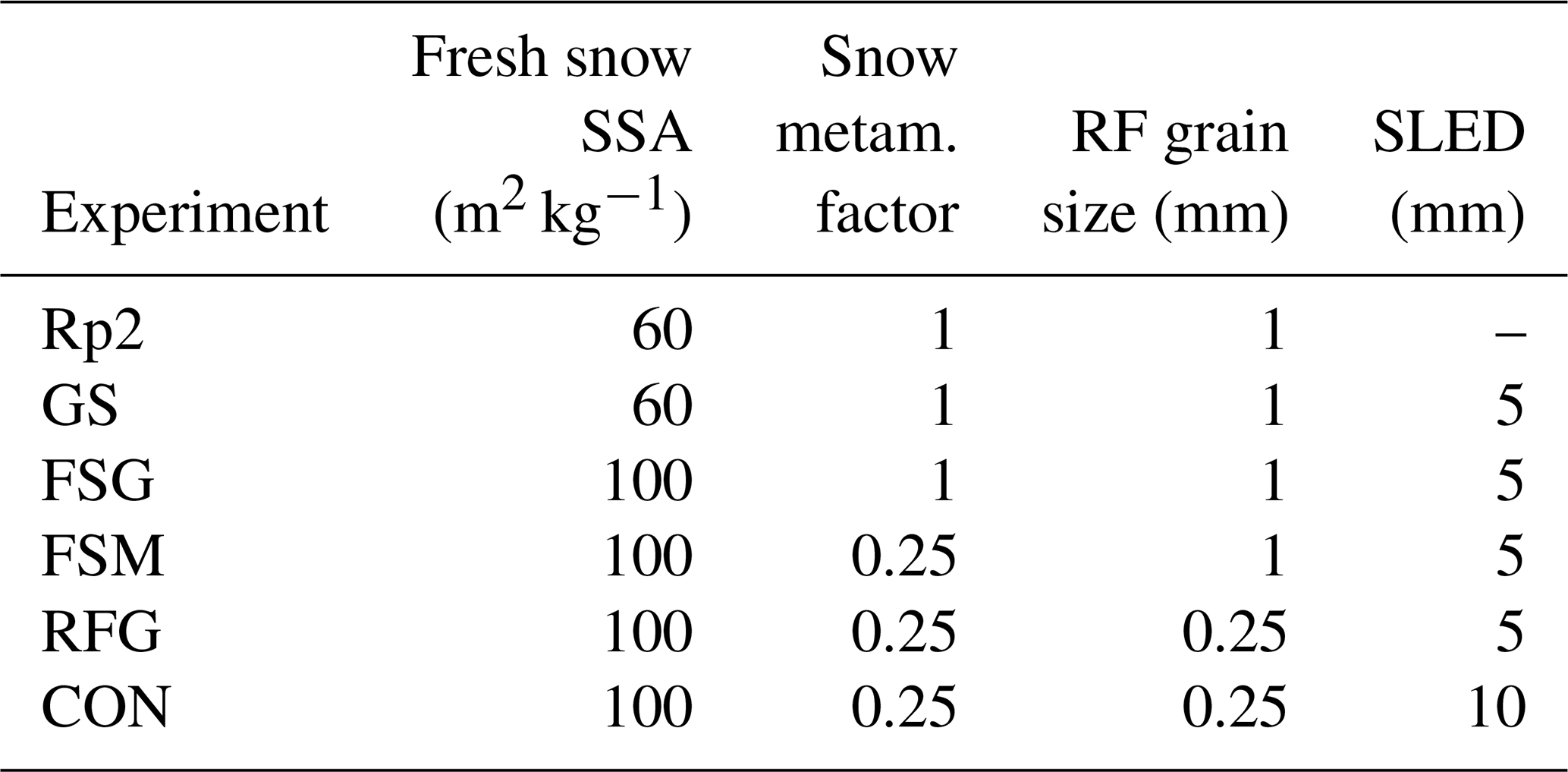
Table 1 summarizes the sensitivity experiments. The settings of the first Rp3 experiment, the Greenland settings experiment (GS), are the same as used for investigating the Greenland ice sheet by Van Dalum et al. (2021b). Rp2 uses the same settings as GS: a fresh snow SSA of 60 m2 kg−1, no snow metamorphism tuning, i.e., α in Eq. (1) set to 1, and a grain size of refrozen water of 1 mm. In GS, we kept the SLED at 5 mm as has been used for the Greenland ice sheet simulations of (Van Dalum et al., 2021b). In Rp2, the SLED is not defined, as no radiation penetration occurs and all absorbed shortwave radiation contributes to the SEB.
Four more experiments are performed using Rp3, changing one parameter at a time. In the fresh snow grain size (FSG) experiment, the fresh snow SSA is increased from 60 to 100 m2 kg−1, reducing r from 55 to 37 µm. An SSA of 100 m2 kg−1 better matches observations of fresh snow at Dome C (Libois et al., 2015). Furthermore, this changes the dry snow metamorphism rate from the fastest to the slowest regime, reducing snow growth by an order of magnitude (Fig. 1). This current parameterization, however, is not optimized for Antarctic conditions, as the observations by Legagneux et al. (2004), on which the parameterization is based, were measured in the French Alps. The temperature of the snow samples is relatively high compared to typical Antarctic temperatures, between 0 and −5.6 ∘C, and they were stored in −15 ∘C. As snow metamorphism is faster for higher temperatures, the snow metamorphism scheme is therefore not directly applicable to the AIS. Hence, in the next experiment we reduce fresh dry snow metamorphism (FSM) even more by setting the tuning parameter α in Eq. (1) to 0.25. This reduces fresh snow metamorphism considerably, but its impact diminishes with increasing SSA (Fig. 1). As grain size significantly impacts the albedo (Gardner and Sharp, 2010; He and Flanner, 2020), slower snow metamorphism reduces shortwave radiation absorption in the snowpack; hence, snow temperatures are expected to decrease. We also reduce the grain size of refrozen snow from 1 to 0.25 mm (RFG), fitting better with Antarctic observations (Domine et al., 2007), which is expected to further reduce melt. The final experiment is the control run (CON), where the SLED is increased to 10 mm following the scale analysis of Van Dalum et al. (2021b) to better conform to a model time step of 6 min. This adjusted SLED takes away the slight overestimation of subsurface heating introduced by using a SLED of 5 mm.
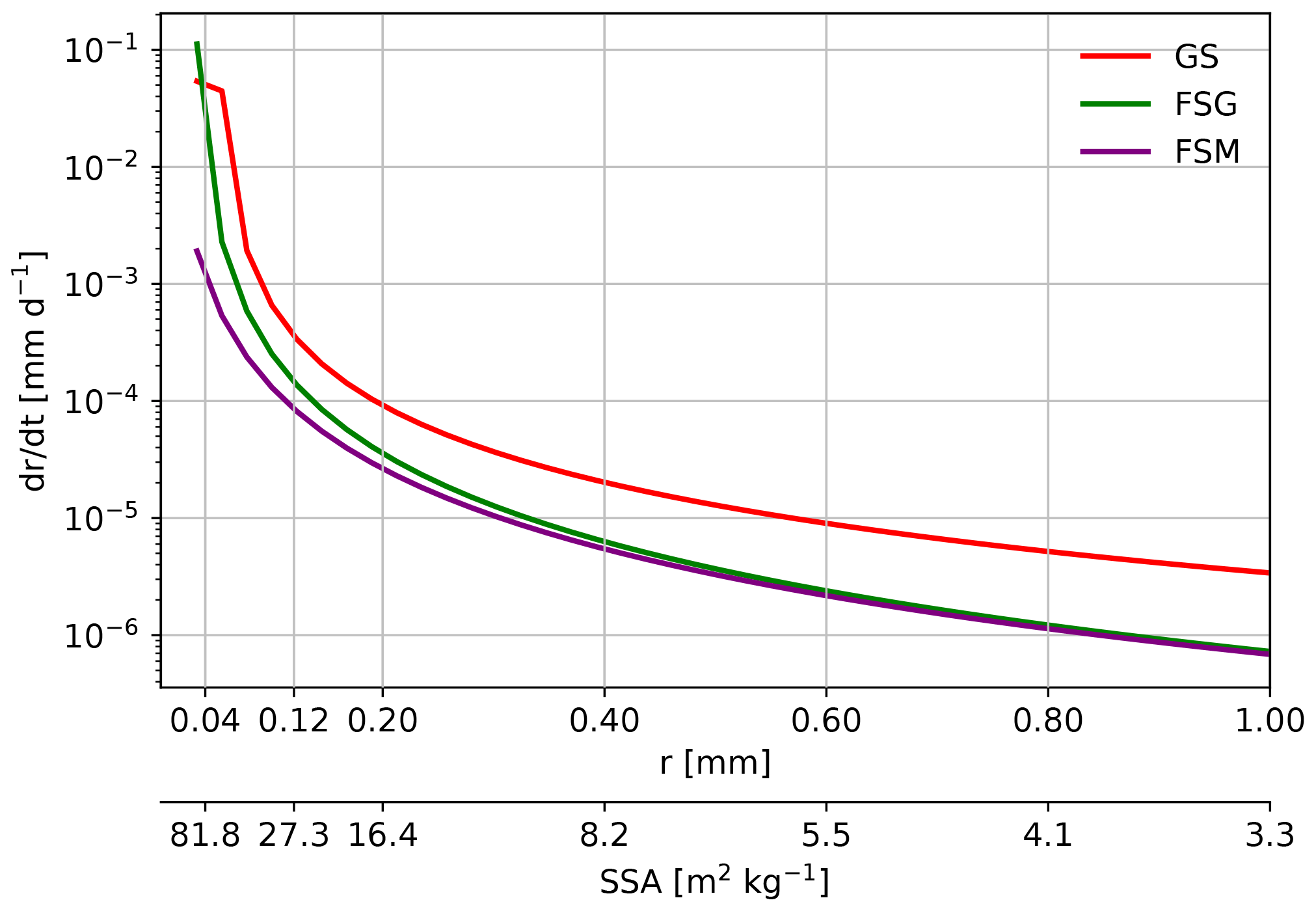
Figure 1Dry snow grain growth as a function of grain radius (r) and specific surface area (SSA) for the Rp3 experiments GS, FSG and FSM.
Running these experiments is computationally demanding; hence, only Rp2, GS and CON are run for the full time period: 1979–2018. FSG, FSM and RFG are run for 1979–1990. For all experiments, 1979–1984 is considered as spin-up, as this time is required to build up a proper snowpack required for the albedo calculations and to limit the impact of initialization on the temperature. Significance between model versions or observations is determined by using statistical bootstrapping with 2-standard-deviation significance.
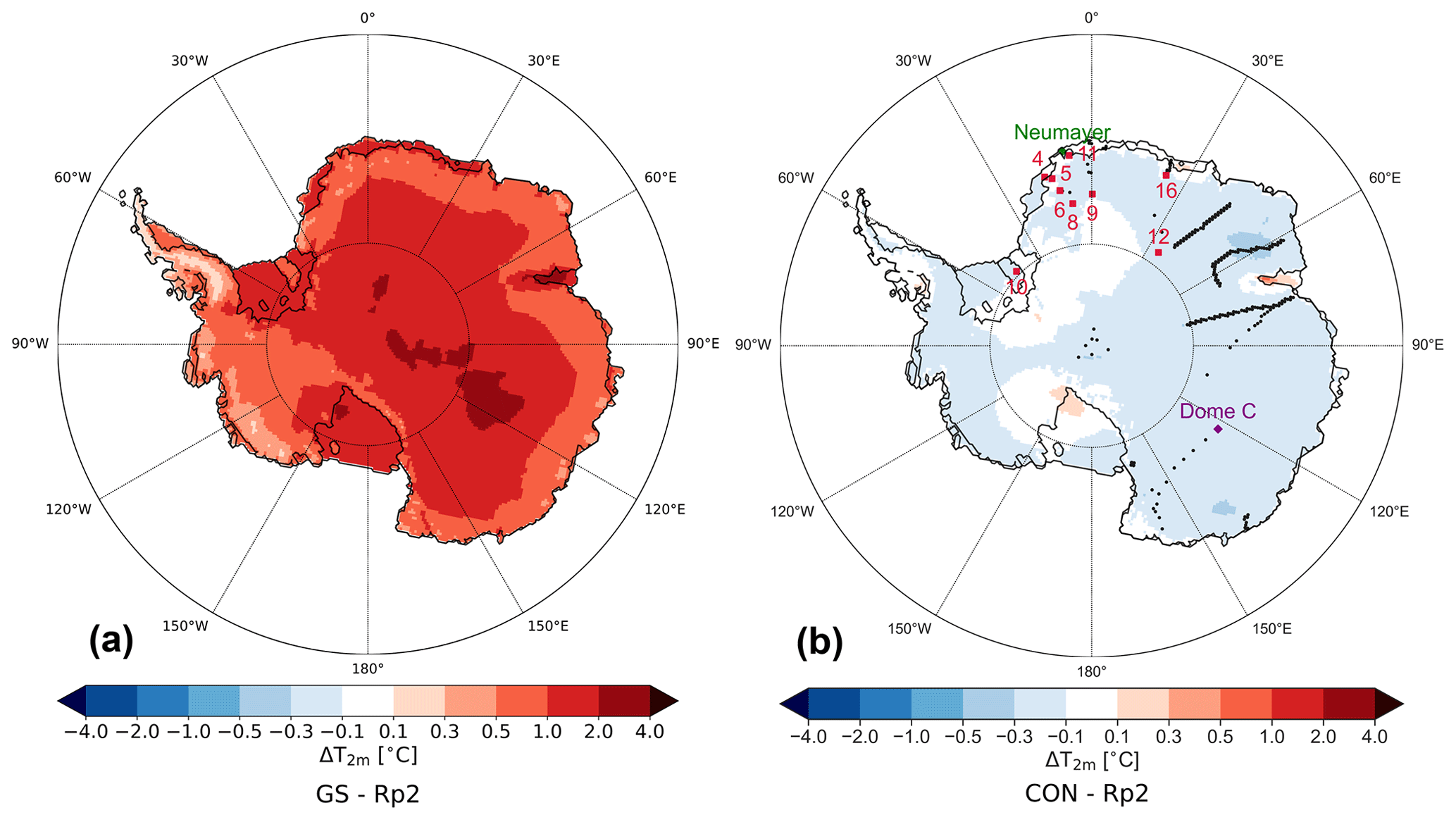
Figure 2Mean yearly-averaged 2 m temperature (T2 m) difference with Rp2 for (a) GS and (b) CON for 1985–2018, with positive values indicating a temperature increase with respect to Rp2. SMB measurement locations are shown in black, the numbered AWS in red, Neumayer in green and Dome C in purple.
2.4 Observational data
In this study, we use several observational data sets to evaluate the SMB and SEB components, snow and 2 m air temperature, 10 m wind speed, and SSA. Here, we provide a brief overview of the observational data sets.
2.4.1 Surface mass balance
Modeled SMB is compared with 1924 SMB measurements including isolated observations and traverses on the EAIS (Fig. 2b). Wang (2021) and Wang et al. (2021) describe this data set in more detail. In addition, melt fluxes are compared with the output of the surface energy balance model (EBM) of Jakobs et al. (2019). This model is forced with high-quality meteorological and radiation observations to specifically produce a melt-rate estimate for Neumayer station (locations shown in Fig. 2b). Neumayer station is representative for ice shelves surrounding the EAIS, as it is located on one of them.
2.4.2 Automatic weather stations
The SEB components, 10 m wind speed and 2 m temperature, are evaluated using automatic weather station (AWS) data of nine stations, most of them located in DML (Fig. 2b). Some are located on an ice shelf (4, 11) or close to the ice-sheet margin (5, 16), and others are more inland, hence covering several climatic regimes. All data are monthly averaged. Van Wessem et al. (2018) provide a more detailed overview of the AWS specifications.
2.4.3 QuikSCAT melt fluxes
The time series of the satellite radar backscatter from the SeaWinds scatterometer aboard QuikSCAT (QSCAT) is used to produce a seasonal meltwater product covering the entire AIS (Trusel et al., 2013). This melt product uses an empirical relation between the satellite product and in situ observations. The QSCAT melt product is provided on a 4.45 km resolution grid but is resampled to the Rp3 grid with the nearest-neighbor method. Here, we use QSCAT to evaluate the modeled ice-sheet-wide surface meltwater fluxes between 2000–2009.
2.4.4 Subsurface snow temperature
Snow temperatures of Rp3 are compared to temperature probe measurements that provide hourly snow temperatures at various depths at Dome C during December 2006 (location shown in Fig. 2b) (Brucker et al., 2011). Probes are positioned down to 21 m depth, but as the upper 20 model layers are always located within 2 m, we limit the evaluation to this depth. Temperatures are measured every 10 cm starting between 10 and 60 cm depth and every 20 cm between 80 and 200 cm.
2.4.5 Specific surface area
The SSA of the upper snow layers at Dome C are retrieved by Picard et al. (2016) between 2013 and 2015 by using an algorithm applied to observed spectral albedos. This SSA product is representative for the upper 2 cm, as the albedo for such a vertically homogeneous snow layer, with an SSA of 50 m2 kg−1 or larger, is representative for more than 95 % of the observed surface albedo (Fig. 1. of Picard et al., 2016). Measurements are available between September and March.
Table 2Statistics of the monthly-averaged downward, upward, and net longwave and shortwave fluxes during summer (LWd, LWu, LWn, SWd, SWu, SWn, respectively), albedo, sensible heat flux (SHF), latent heat flux (LHF), 2 m temperature (T2 m), skin temperature (Tskin), and 10 m wind speed (V10 m) using AWS data of DML between 1997 and 2012 (locations shown in Fig. 2b). We use the ratio of the monthly sum of SWu and SWd to determine the albedo. For all variables, 202 observations are available. The correlation coefficient (R2), bias and root-mean-square error (RMSE) are shown for Rp2, GS and CON. In all following figures, Rp2 is in black, GS in red and CON is in blue.
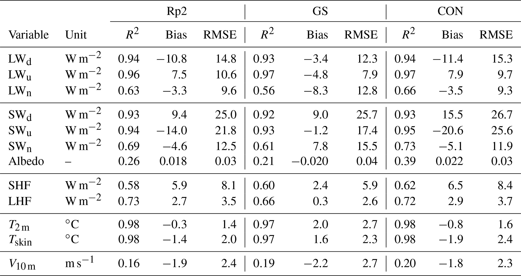
Figure 2 shows the yearly-averaged T2 m difference for GS and CON with Rp2. Considerably higher temperatures are simulated in GS, with some areas more than 2.0 ∘C warmer with respect to Rp2. The temperature in CON (Fig. 2b) is on average only 0.1 to 0.3 ∘C lower than Rp2. In summer (Fig. A1), the signal of Fig. 2 is amplified. A comparison with observations in DML during summer (Table 2, Fig. A2), which is the season where any changes in the albedo have the strongest impact on the SEB, shows that the temperature of Rp2 is modeled well, with a small bias of −0.3 ∘C and a root-mean-square error (RMSE) of 1.4 ∘C. The bias of GS and CON is larger: 2.0 and −0.8 ∘C respectively. For more inland stations like station 8, 9 and 12, the bias of GS is larger compared to stations close the edge of the ice sheet, while the bias of Rp2 and CON is smaller. This illustrates the high sensitivity to the implemented changes on the T2 m for the AIS in Rp3. The new snow albedo and radiative transfer scheme results in a lower albedo, which is especially important during summer and will be discussed in more detail in Sect. 5. Including radiation penetration leads to higher subsurface snow temperatures, enhancing snow metamorphism and subsequently enhancing radiation absorption. Due to this positive feedback, inaccuracies in the modeled (sub)surface snow metamorphism (Flanner and Zender, 2006) are amplified in Rp3.
To investigate the exact cause of deviating temperatures, we show the yearly-averaged T2 m difference with Rp2 for all sensitivity experiments for 1985–1990 (Fig. 3). As Van Wessem et al. (2018) have shown that Rp2 models T2 m fairly well, it is therefore used as a benchmark. Similar to Fig. 2, the temperature of GS is overestimated significantly. All subsequently implemented changes lower the temperature, although some changes impact it more than others. A significant lowering of the temperature is induced by the increase in the fresh snow SSA to 100 m2 kg−1 in the FSG experiment (Fig. 3b). FSG also uses a different fresh snow regime in the grain growth parameterization (Sect. 2.1, Fig. 1), and grains with a high SSA consequently remain at the surface for longer. The temperature, however, is still too high.
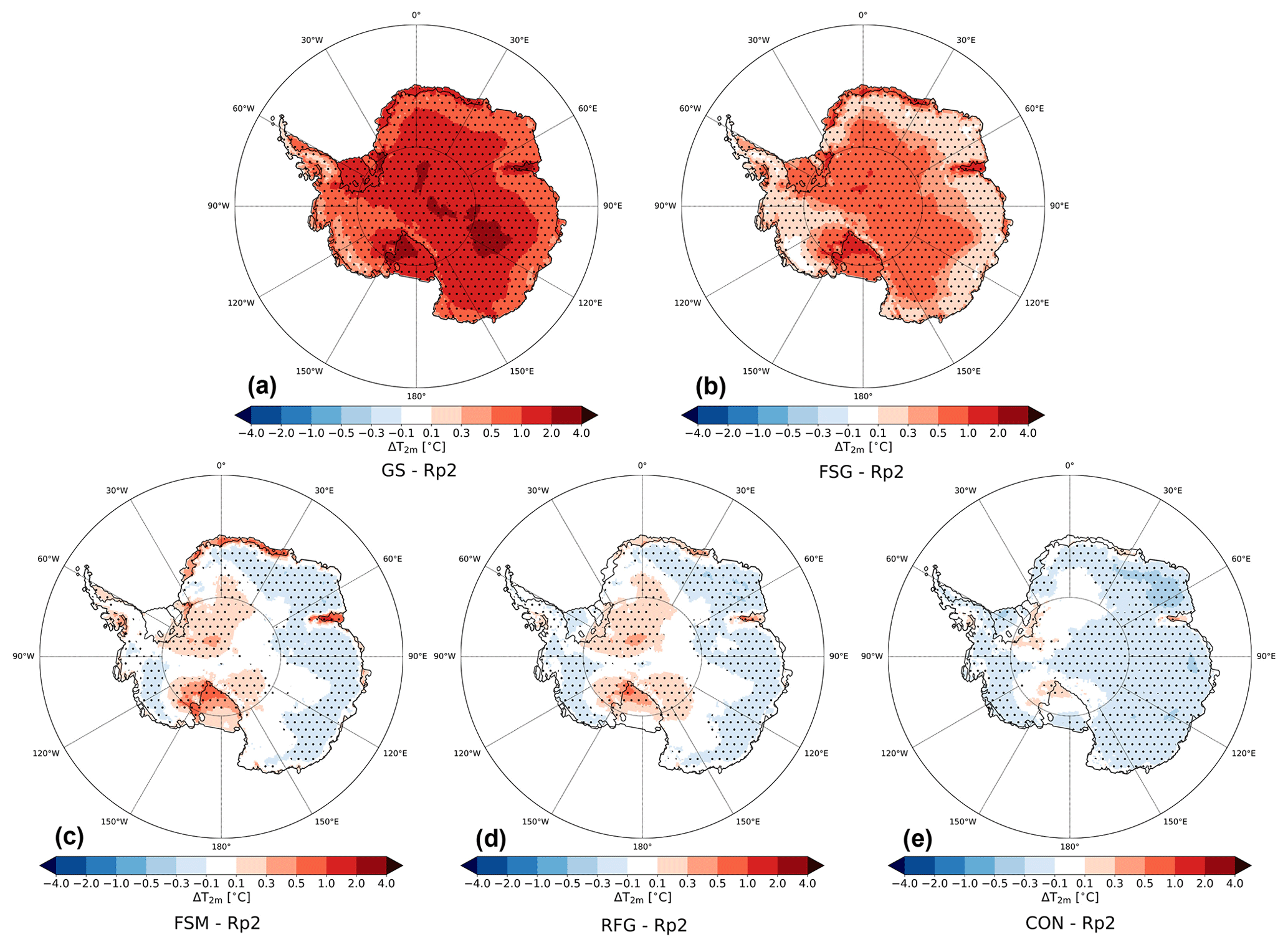
Figure 3Mean yearly-averaged 2 m temperature (T2m) difference with Rp2 for (a) GS, (b) FSG, (c) FSM, (d) RFG and (e) CON for 1985–1990. The dots represent significance.
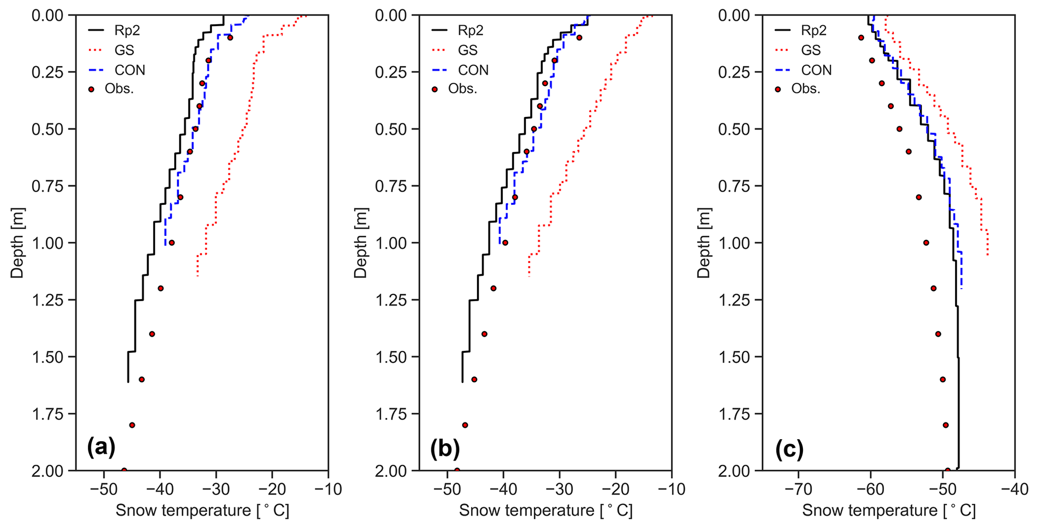
Figure 4Subsurface snow temperature profile for Dome C in 2007 for the 20 upper snow layers of Rp2, GS and CON and observations (Obs.) for (a) 5 January, (b) 17 January and (c) 5 April, all measured at 06:00 UTC (14:00 LT).
The strongest temperature lowering occurs when we further reduce the fresh dry snow metamorphism (Fig. 3c) by implementing a tuning parameter (Eq. 1). As Fig. 1 illustrates, this tuning reduces in particular the snow metamorphism for small grains, i.e., up to 100 times slower metamorphism in FSM than FSG. This tuning makes that surface layers with a high SSA (>50 m2 kg−1) are more persistent between snow deposition events, consequently lowering the surface temperature and hence, through turbulent and longwave exchange between the surface and near-surface atmosphere, reducing T2 m. The significant temperature differences between Fig. 3a and c show how sensitive Rp3 is to grain size and underline the importance of an accurate snow metamorphism scheme.
Higher temperatures are relatively persistent on some of the ice shelves (Fig. 3c), especially in DML. These regions are characterized by melt in summer that refreezes in the snowpack. As meltwater refreezes, it increases snow grain size, resulting in more solar radiation absorption and therefore higher temperatures. Reducing the refreezing snow grain size consequently reduces the temperature difference on relatively dry locations with melt (Fig. 3d). Increasing the SLED further lowers the temperature as subsurface heating is reduced (Fig. 3e). The temperature in CON is now somewhat too low during summer (Table 2). This bias can be further reduced by slightly changing α in Eq. (1).
3.1 Snow temperature
An important addition in Rp3 is subsurface penetration of shortwave radiation, which allows subsurface absorption and local heating of the snowpack. For the Greenland ice sheet, Van Dalum et al. (2021b) showed that Rp3 models higher subsurface snow temperatures, as a result of internal heating, that match well with observations at Summit. In the ablation zone, the melting point is reached to a greater depth than in Rp2, enabling subsurface melt. Here, we show that the snow temperatures of CON match well with observations (Brucker et al., 2011) at Dome C (Fig. 4). During summer (Fig. 4a and b), we observe that Rp2 is somewhat too cold compared to measurements. The snow temperatures of GS are significantly overestimated by up to 10 ∘C. During autumn (Fig. 4c), temperature profiles of Rp2 and CON, and to a lesser extent GS, are more similar, as surface temperature differences are smaller and the impact of radiation penetration diminishes towards winter (Van Dalum et al., 2021b). Compared to observations, however, temperatures in autumn are too high for this particular year.
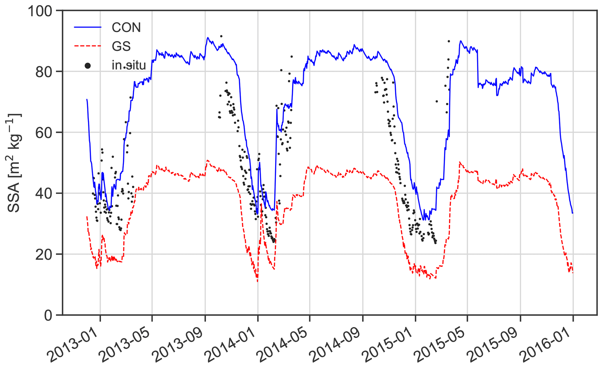
Figure 5Time series of average SSA for Dome C of the upper 2 cm of the snowpack in CON and GS and as observed by Picard et al. (2016).
In the previous section, we illustrated the importance of grain size on the temperature of the AIS. Compared to in situ observations at Dome C (Picard et al., 2016), the SSA of the upper 2 cm in the CON simulation follows the yearly cycle well (Fig. 5). The SSA drops gradually over time during spring and summer to values around 40 m2 kg−1, which is somewhat higher than observed. In GS, the SSA is too low as it drops below 20 m2 kg−1. The SSA decline during spring is delayed by a few weeks, but the rate of change is similar to observations. After summer, the SSA gradually increases with deposition of fresh snow but only reaches 40 to 50 m2 kg−1 for GS, significantly below observations. For CON, the SSA gradually increases to 80 to 90 m2 kg−1, which is in agreement with observations. Note that the average SSA of the upper 2 cm never reaches the prescribed fresh snow SSA of 100 m2 kg−1, as large snowfall events at this polar desert site are rare (Picard et al., 2019). To summarize, the GS settings lead to unrealistically low SSAs. The CON settings somewhat underestimate snow metamorphism, leading to higher SSA during summer, but this can be fine-tuned using α in Eq. (1). Increasing α results in an SSA evolution, depending of the choice of α, to be between FSG (which uses α=1) and FSM (which uses α=0.25) in Fig. 1.

Figure 6Bias of monthly-averaged downward and upward longwave and shortwave fluxes during summer (LWd, LWu, SWd, SWu, respectively), sensible heat flux (SHF), and latent heat flux (LHF) using AWS data of DML between 1997 and 2012. Each numbered circle chart represents an AWS (locations shown in Fig. 2b) and is split into three parts: the upper right shows the bias of Rp2 with observations, the lower right GS and the left CON.
Table 2 shows the statistics of SEB components compared to AWS observations in summer from DML in Rp2, GS and CON. All fluxes toward the surface are defined positive.
The longwave radiation of Rp2 and CON correlate well with observations, but some biases are observed. The underestimation of LWd illustrates that the atmosphere is too cold in the model. This could be due to too few clouds, too low atmospheric humidity or biases in the radiation scheme for these cold conditions. This is partly compensated for by underestimated LWu, resulting in a relatively small LWn bias. In GS, the bias of LWn is larger, as higher surface temperatures lead to an overestimation of LWu, while only partly compensated for by increased LWd. Bias differences between most stations are limited, especially close to the edge of the ice sheet (Fig. 6a, b). For station 12 that is located on the Antarctic Plateau, both LWd and LWu are overestimated for Rp2 and CON.
Table 2 shows that SWd is overestimated for all model experiments. As no parameters that directly impact SWd have been changed, it illustrates that the atmosphere is too transparent, likely due to similar reasons as causing the LWd differences. For Rp2 and CON, this bias is compensated for by SWu, as the albedo is somewhat too high during summer. Table 2 also shows that the albedo of GS is on average too low, which is discussed in more detail in Sect. 5.1, resulting in a lower compensating SWu and consequently a larger SWn bias. Similar to longwave radiation, the biases of most stations are similar, except for station 12, where SWd and SWu are underestimated (Fig. 6d, e).
On average, the SHF is overestimated during summer, despite an underestimation of the wind speed (V10 m, Table 2). The SHF overestimation is stronger for station 16 and for more inland stations like station 8 and 12 (Fig. 6f). This can be either due to an incorrect representation of the roughness length or an incorrect temperature gradient between surface and atmosphere. In GS, turbulent heat exchange is smaller while T2 m is overestimated. For a stable surface layer, this therefore suggests that the temperature of lower atmospheric layers is too high in the model. Similarly, GS also shows a better LHF representation than Rp2 and CON (Table 2 and Fig. 6c). Hence, turbulent fluxes can still be further improved.
5.1 Albedo
Year-round monthly-averaged albedo in DML compared to observations is shown in Fig. 7. Figure 7a illustrates that the spread in data points in GS is similar to CON but with a lower average. Moreover, an albedo lower than 0.8 is sometimes modeled in GS and is shown by observations, while it is absent in Rp2 and CON (Fig. 7b).
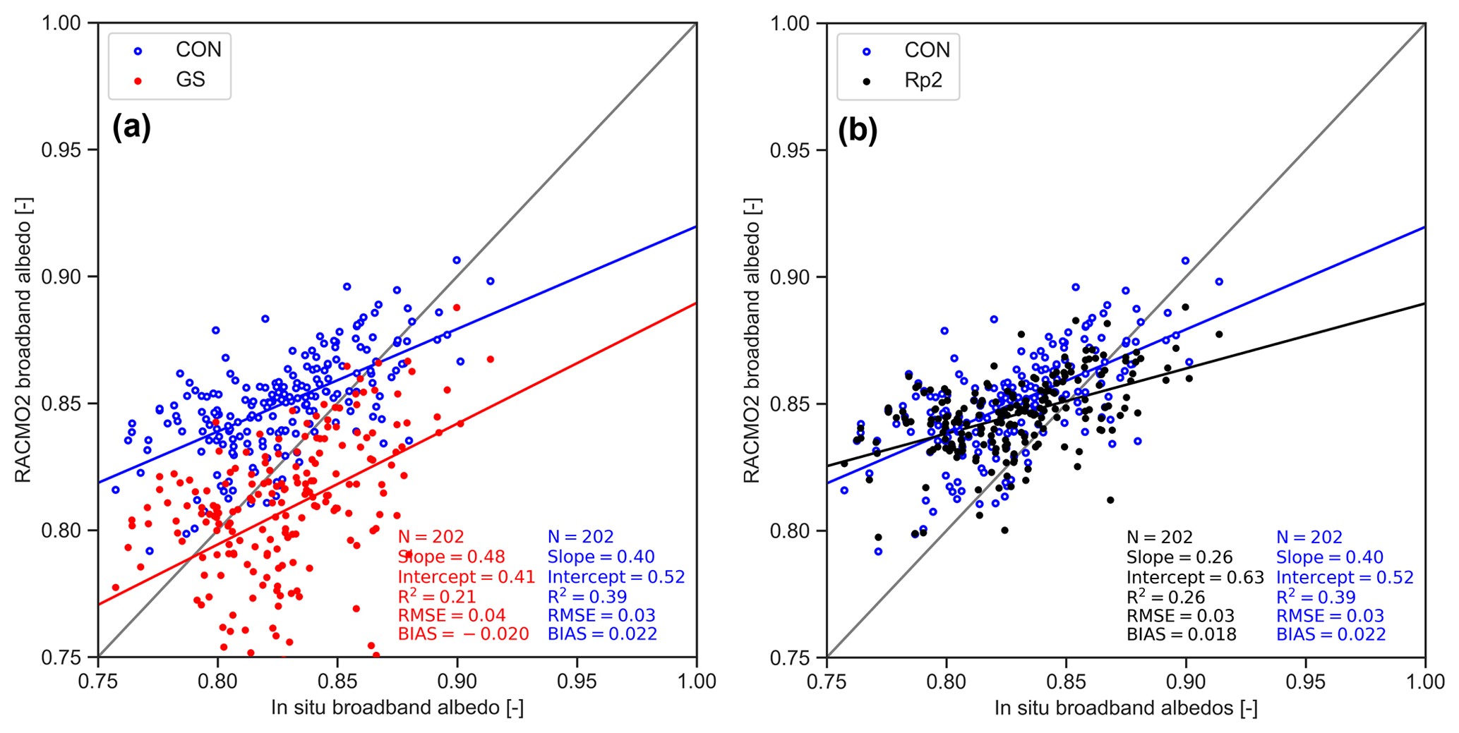
Figure 7Monthly-averaged albedo in DML in (a) CON and GS and (b) CON and Rp2 compared to AWS measurements between 1997 and 2012. The gray lines are the one-on-one lines, and the red and blue lines are linear regression of the data, with the number of observations (N), the slope, the intercept, the correlation coefficient (R2), the bias and root-mean-square error (RMSE).
Yearly averaged, the albedo of CON is relatively homogeneous over the AIS (Fig. 8a) with a high albedo (>0.8) almost everywhere due to the abundance of fine-grained snow. Compared to Rp2, the differences are generally small, with somewhat higher albedos in West Antarctica (Fig. 8c). The albedo of GS is significantly lower than Rp2 (Fig. 8b), showing the impact of snow properties on the radiative transfer scheme in Rp3. The largest differences in both GS and CON are observed for the Amery ice shelf, where bare ice can be found at the surface during summer. The transition from snow to bare ice is faster due to higher snow temperatures, leading to more snow-free days and consequently a lower mean albedo. Note that the albedo in Rp2 is fixed for bare ice, while TARTES and SNOWBAL are called in Rp3, allowing a variable ice albedo depending on atmospheric conditions (Van Dalum et al., 2020).
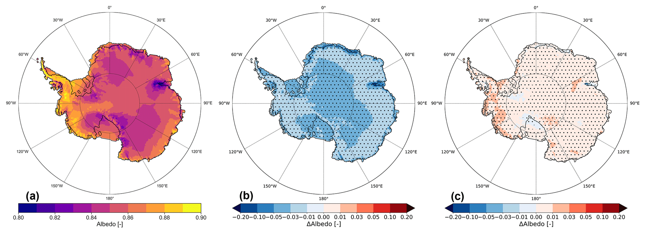
Figure 8(a) Mean yearly-averaged albedo in CON and albedo difference with Rp2 in (b) GS and (c) CON for 1985–2018. The dots represent significance.
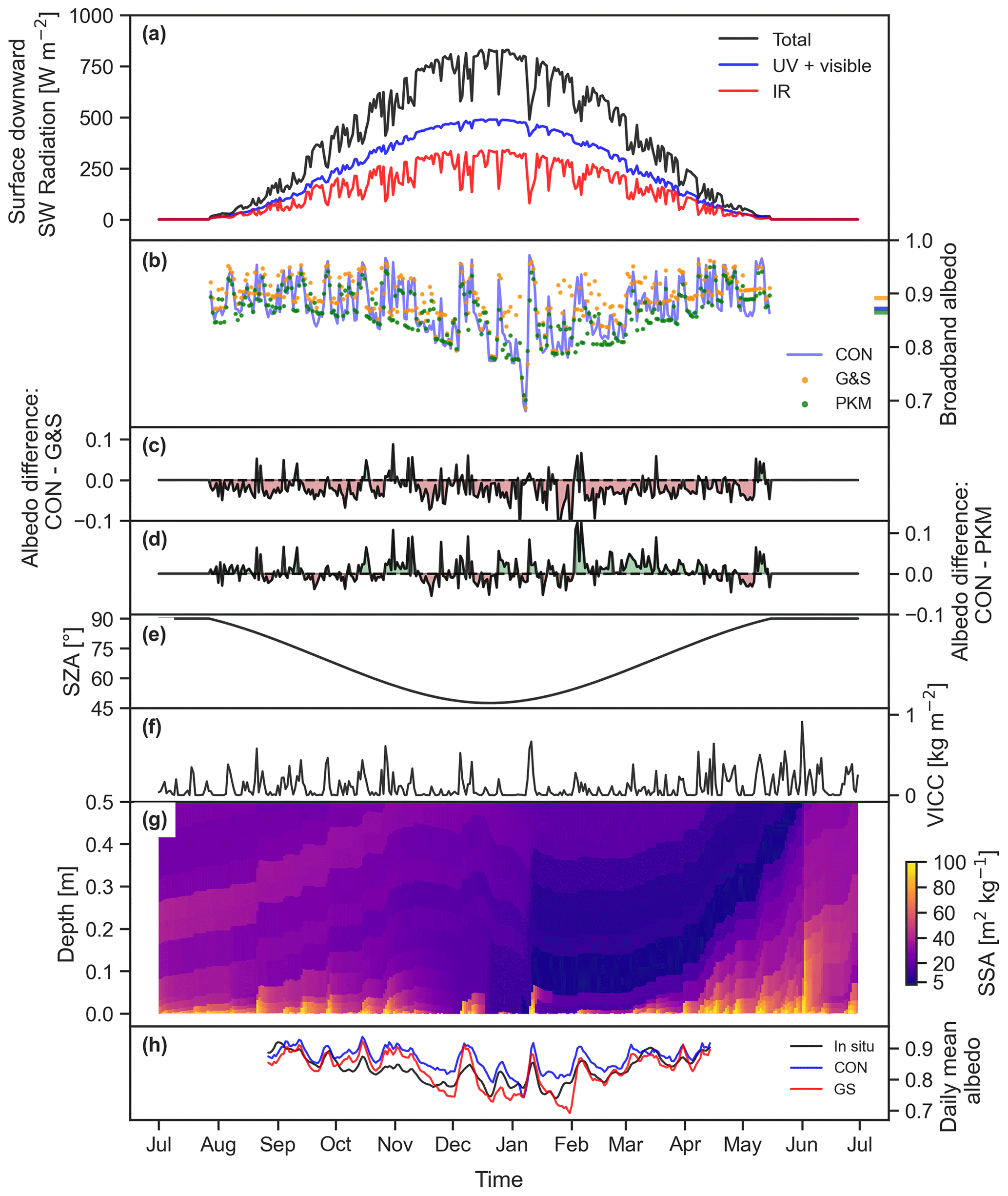
Figure 9Time series at Neumayer for 2012–2013, 12:00 UTC (12:00 LT). (a) Instantaneous surface downward shortwave radiation, split into infrared (IR), ultraviolet (UV) and visible radiation; (b) instantaneous broadband albedo for CON, the parameterization of Gardner and Sharp (2010) (G&S) and Kuipers Munneke et al. (2011) (PKM). The horizontal lines on the right indicate the mean. (c) Albedo difference CON – G&S and (d) CON – PKM; (e) solar zenith angle (SZA); (f) vertically integrated cloud cover (VICC), which is the summation of the liquid and ice water path; (g) SSA as a function of depth for CON and (h) daily mean albedo for CON, GS and in situ observations.
5.2 Neumayer case study
Figure 9 shows a case study at Neumayer for the 1-year period July 2012 to July 2013 at local noon, illustrating the various processes that impact the albedo on seasonal and sub-seasonal timescales. In general the albedo is high (close to 0.9, Fig. 9b) but fluctuating, mostly depending on cloud cover (Fig. 9f). The albedo is on average lower than the broadband albedo parameterization of Gardner and Sharp (2010) (G&S, Fig. 9c) employed in Rp2. Simulating radiation penetration by applying a simple exponential decay function with depth for radiation to G&S, as Kuipers Munneke et al. (2011) (PKM) did, lowers the albedo, reducing the difference with CON. This illustrates the importance of radiation penetration even with the presence of fresh snow during most months (Fig. 9g). The removal of fresh snow by sublimation during summer does not lead to considerable differences with G&S and PKM. The addition of a thin snow layer (only millimeters thick) on top of firn in February, on the other hand, induces a strong albedo increase, resulting in a large albedo difference of more than 0.1 with PKM (Fig. 9d). Such differences reduce over time when snow metamorphism occurs or if more fresh snow is deposited. This illustrates that a simple exponential decay function is not enough to properly capture radiation penetration.
The impact of cloud cover on irradiance is shown in Fig. 9a. It shows that infrared (IR) radiation is filtered out by clouds but that cloud content (Fig. 9f) is too small to considerably impact UV and visible irradiance. As the spectral albedo of IR radiation is low (Dang et al., 2015; Warren, 2019), the broadband albedo in Rp3 consequently increases with increasing cloud content. Compared to G&S and PKM, cloud cover induces stronger albedo variations in CON, as this effect is now explicitly taken into account.
Solar zenith angle (SZA) also impacts the albedo. The albedo increases with SZA, as it increases the angle of incidence of radiation, leading to a higher likelihood for light to scatter out of the snowpack (Solomon et al., 1987; Gardner and Sharp, 2010). The spectral distribution of light also changes with increasing SZA. For high SZA (>80∘), a relatively larger part of the irradiance is IR (Fig. 9a), for which the spectral albedo is low, partly compensating the albedo increase. This effect, however, is not captured in G&S and PKM but is included in Rp3. Consequently, the albedo is lower for CON for high SZA, as can be seen at the beginning of May during clear-sky conditions (Fig. 9c, d). Monthly averaged, however, the aforementioned processes have a limited effect, as most differences between CON and Rp2 are averaged out (Fig. 7b).
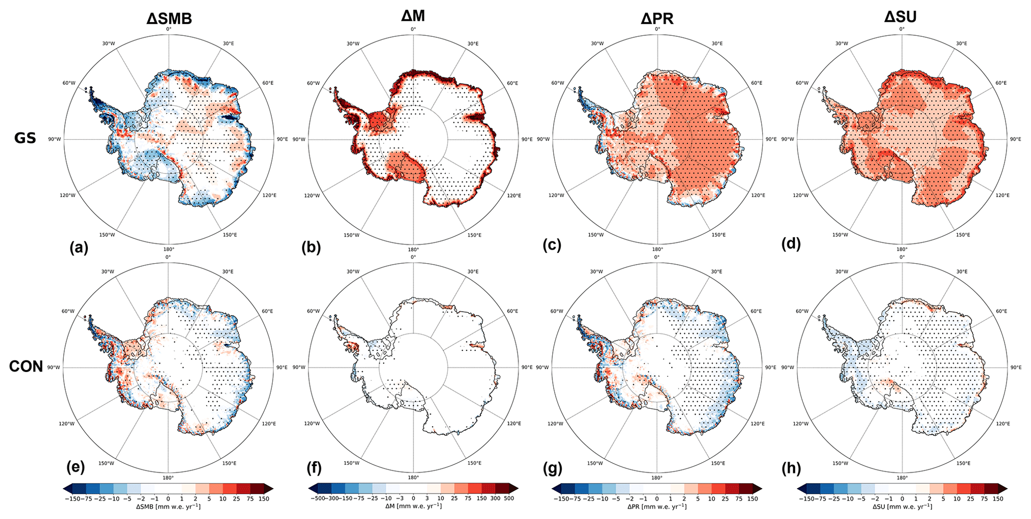
Figure 10Yearly accumulated SMB, melt (M), precipitation (PR) and sublimation (SU) difference with Rp2 for GS (a–d, respectively) and CON (e–h, respectively) for 1985–2018, with positive values showing an increase with respect to Rp2. Runoff and drifting snow erosion are not shown. The dots represent significance.
Compared to observations, the daily mean albedo product of CON is often too high (Fig. 9h), especially during spring and summer, while the albedo of GS is often too low during summer and too high during spring. To summarize, tuning the snow layers to better fit with SSA observations (Fig. 5) and temperature (Fig. 3) does not necessarily lead to a smaller bias in the SEB components or albedo. The analysis of the SEB shows that there are some compensating biases, i.e., clouds and turbulence. Despite on average only minor albedo changes between CON and Rp2 (Fig. 7), we also show by analyzing a case study for Neumayer that with the introduction of a new physically based snow albedo and radiative transfer scheme the instantaneous albedo can differ considerably. In particular, radiation penetration and spectral shifts due to cloud cover and high SZA lead to high day-to-day albedo variability.
Figure 10 shows the mean yearly-accumulated SMB, melt, precipitation and sublimation difference with Rp2 for GS (upper row) and CON (lower row). In CON, the SMB differences are generally small (lower than 10 mm w.e. yr−1), with somewhat larger differences for the West Antarctic ice sheet (WAIS) and the AP that are driven by precipitation changes. The precipitation changes are minor, however, as total precipitation for the WAIS and AP are more than an order of magnitude larger (Van Wessem et al., 2016). Melt has increased on the Wilkins, George VI, and northern part of the Larsen C ice shelf in the AP and the Amery ice shelf in East Antarctica. The changes of Rp3 are therefore largest for warm regions where melt is already significant, in agreement with Van Dalum et al. (2020, 2021b). Runoff, however, remains limited (not shown), and almost all meltwater is buffered in the snowpack where it refreezes. Only at the southern part of the Amery ice shelf is the retention capacity now exceeded and runoff modeled, hence lowering the SMB. The margins of DML show considerable year-to-year and spatial melt variability. This demonstrates the high sensitivity of the implemented changes for this region, as the snowpack is close to the melting point in summer and additional energy absorption therefore leads to a stronger meltwater flux.
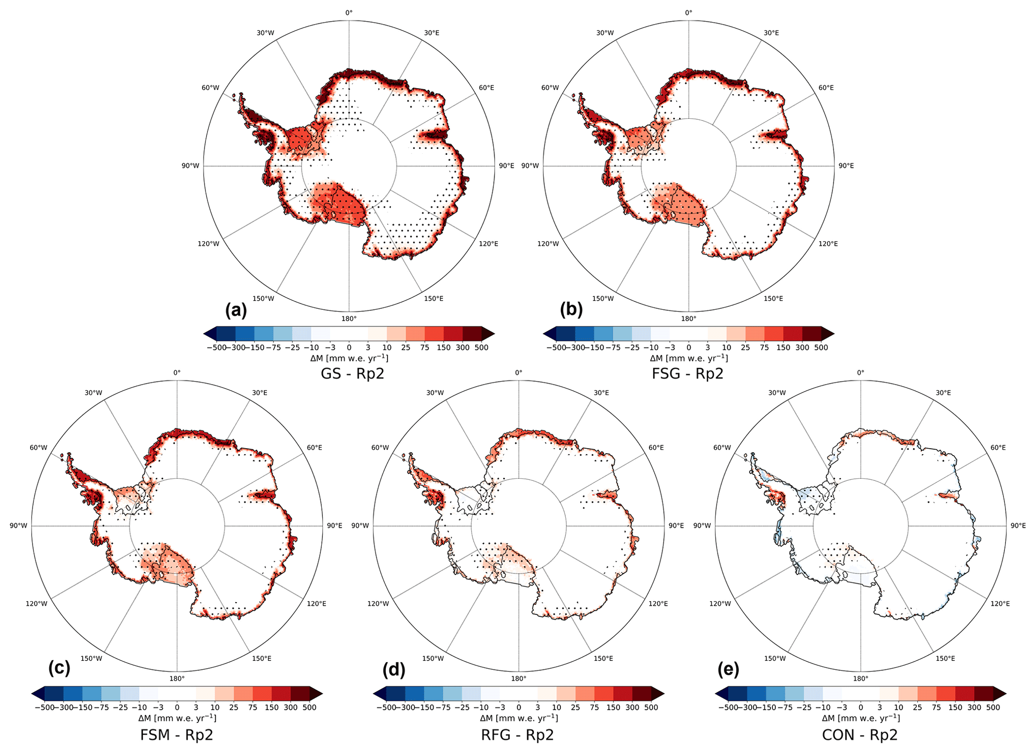
Figure 11Mean yearly-accumulated melt difference with Rp2 in mm w.e. yr−1 for (a) GS, (b) FSG, (c) FSM, (d) RFG and (e) CON for 1985–1990. Positive values show a melt increase with respect to Rp2. The dots represent significance.
In GS (upper row of Fig. 10), a strong SMB decrease is modeled for ice shelves in the AP, DML and Amery ice shelf. More inland, the SMB increases somewhat, which is mainly caused by an ice-sheet-wide precipitation increase. It is, however, partially compensated for by more sublimation. As the precipitation parameterization has not been changed, the moisture of this excess precipitation has been taken up locally. Further analysis showed that it relates to unrealistic features during summer in GS. Due to the higher surface temperature, sublimation increases and a cloud-topped shallow convective layer is modeled for the interior of the ice sheet. These clouds subsequently provide the additional precipitation. This synoptic weather pattern is, however, not backed by observations. Furthermore, melt has increased strongly around the margins of the entire AIS and all ice shelves. This melt changes the snow structure and leads to extensive runoff on several smaller ice shelves in DML, where the snowpack is close to saturation in summer, and on the Amery, Larsen C, Wilkins and George VI ice shelves. Finally, compared to 1924 SMB observations in the EAIS (locations shown in Fig. 2b), the difference between CON and GS is small, and both agree well with measurements (Fig. A3), with a bias of 23.5 and 24.4 mm w.e. yr−1 and RMSE of 106.4 and 106.0 mm w.e. yr−1, respectively. The correlation coefficient is 0.41 for both CON and GS.
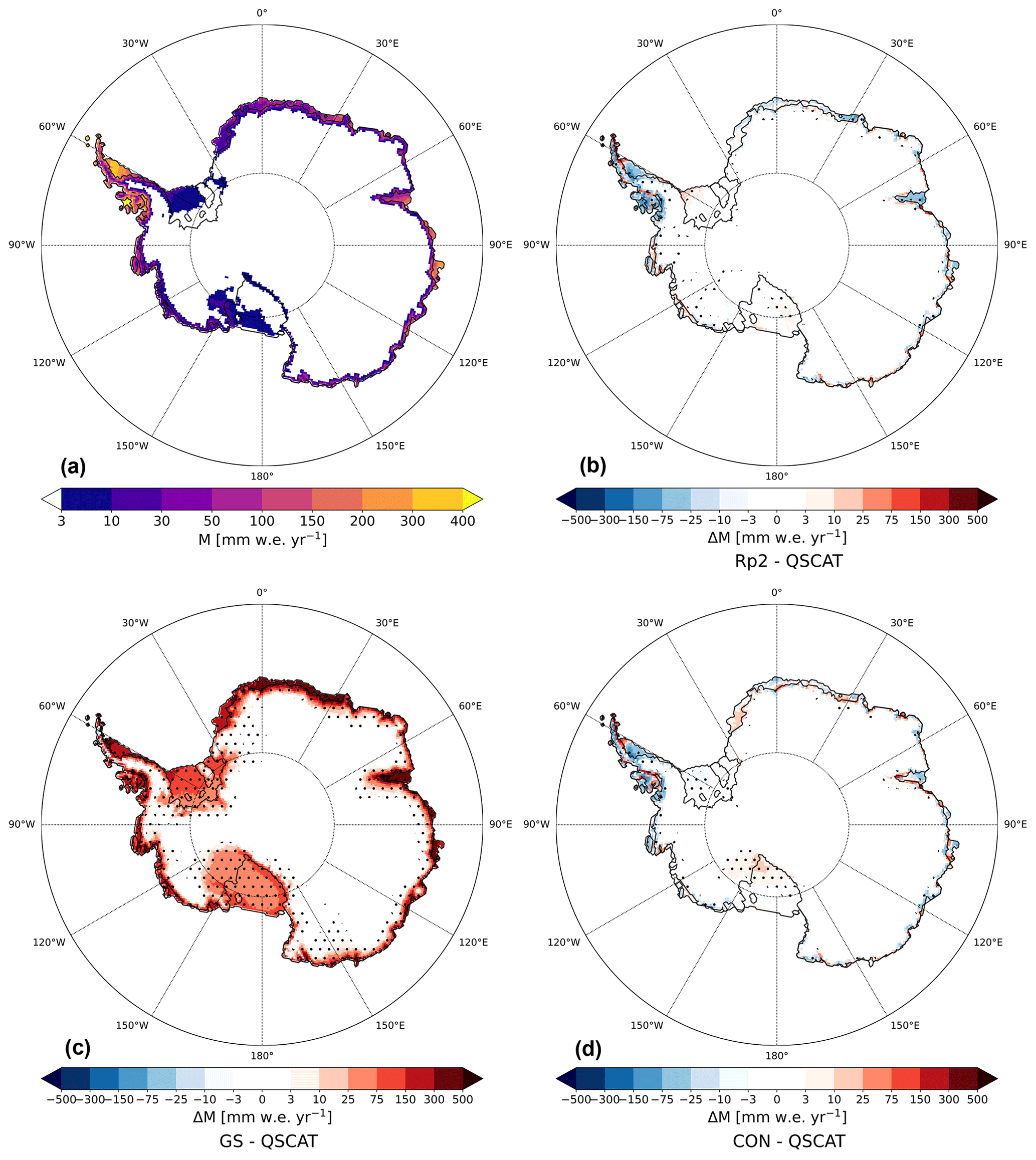
Figure 12(a) Mean yearly-averaged melt in mm w.e. yr−1 estimated by QSCAT; melt difference with QSCAT for (b) Rp2, (c) GS and (d) CON for 2000–2009. For (b)–(d), positive values indicate a melt increase with respect to QSCAT. The dots represent significance.
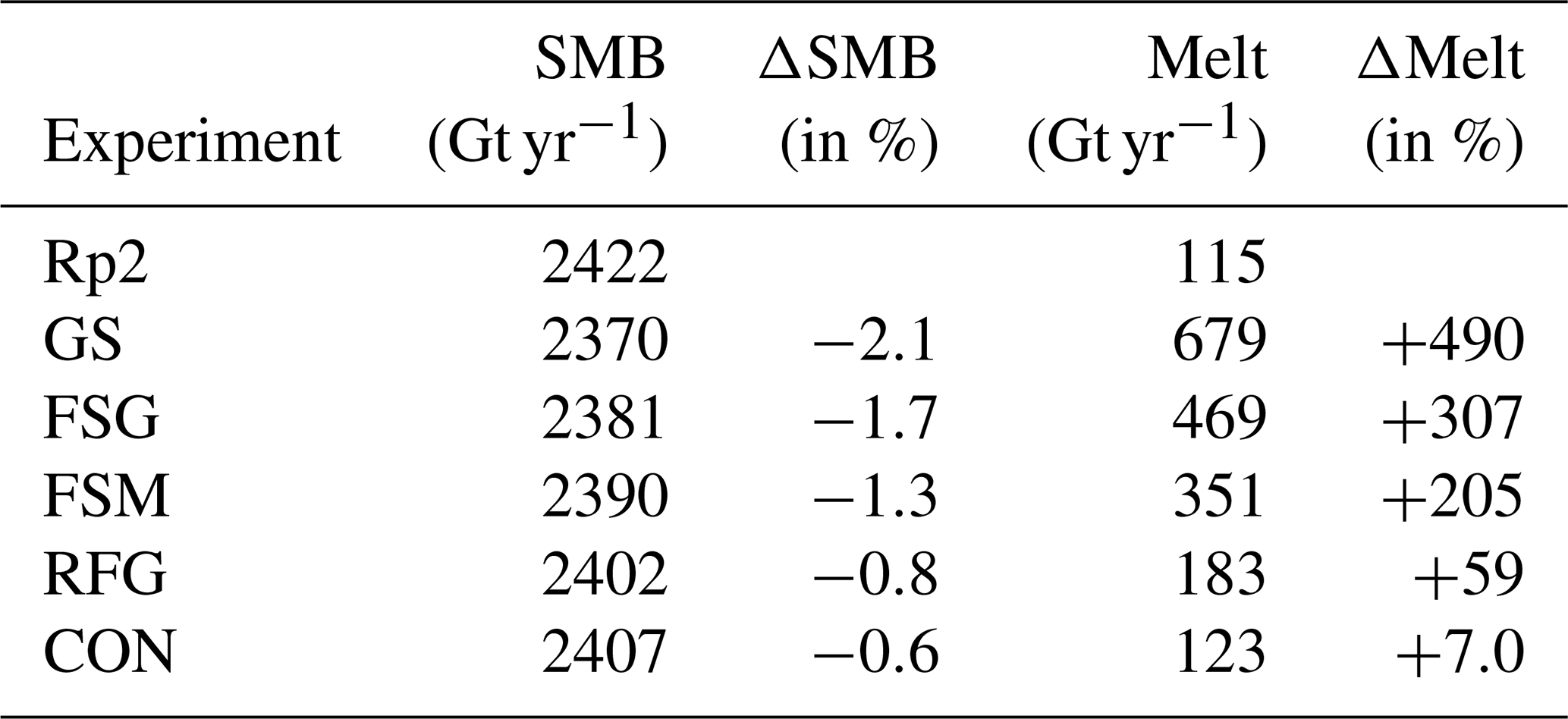
To investigate what causes the strongly overestimated melt in GS, Fig. 11 shows the melt difference with Rp2 for all sensitivity experiments. By increasing the fresh snow SSA (Fig. 11b) and reducing fresh dry snow metamorphism (Fig. 11c), less radiation is absorbed, lowering melt for most regions, in particular for the Ross and Filchner–Ronne ice shelves. These ice shelves are covered by fine-grained snow for most of the year and are therefore especially sensitive to changes in the fresh snow parameterization. The change to the fresh snow SSA and metamorphism delays the onset of the melt season, but its impact diminishes as the melt season progresses. Unsurprisingly, a strong melt reduction occurs by lowering the refreezing grain size (Fig. 11d), which leads to less energy absorption in areas with refreezing. For the time step currently employed in Antarctic simulations, a SLED of 5 mm is on the lower end of the scale analysis that is employed in Van Dalum et al. (2021b). This underestimation of the SLED results in a slightly overestimated heat buffering in the uppermost part of the snow layer, leading to more internal heat absorption. Hence, melt is expected to be further reduced by increasing the SLED. This is indeed the case when comparing RFG (Fig. 11d) with CON (Fig. 11e), illustrating the impact of subsurface heating. Integrated over the AIS, yearly-averaged melt has increased by as much as 490 % in GS with respect to Rp2. Each sensitivity experiment lowers the melt flux, resulting in only a 7.0 % increase in CON (Table A1). As a result, the domain-integrated yearly-averaged SMB modeled in GS is lower (2370 Gt yr−1) than CON (2407 Gt yr−1).
6.1 Melt comparison with QuikSCAT
In this section we compare modeled melt with QSCAT data (Sect. 2.4.3). QSCAT shows that virtually no melt occurs on the majority of the AIS (Fig. 12) and that there are only small melt fluxes (<100 mm w.e. yr−1) around most of the margins of East and West Antarctica. More melt is observed in the AP, especially on the ice shelves, but it is still 1 order of magnitude smaller than observed in the ablation zone of west Greenland (Van den Broeke et al., 2016).
Compared to QSCAT, Rp2 (Fig. 12b) and CON (Fig. 12d) perform generally well, with small differences around the margins of the WAIS and EAIS. In the AP, Rp2 and CON predict more melt in the northern part of Larsen C, while melt is underestimated in the southern part. Furthermore, melt in the western AP appears underestimated. For the Wilkins and George VI ice shelves, however, CON models higher melt fluxes compared to QSCAT, similar to Fig. 10f. The melt in GS (Fig. 12c) is overestimated by more than an order of magnitude for almost all regions close to the ice-sheet margin. Furthermore, GS models a relatively large melt flux for the Ross and Filchner–Ronne ice shelves, where QSCAT observes virtually no melt.
Integrating melt over the AIS shows a similar pattern (Fig. 13), with melt in GS almost an order of magnitude larger than QSCAT in every year. Rp2, on the other hand, compares well with observations. The addition of a new snow albedo and radiative transfer scheme in Rp3 impacts the strong melt–albedo feedback, similar to findings of Jakobs et al. (2019), enhancing melt. Differences with QSCAT are reduced when all changes of the sensitivity experiments are implemented, leading to a better correlation with CON. The interannual variability compares well for all experiments.
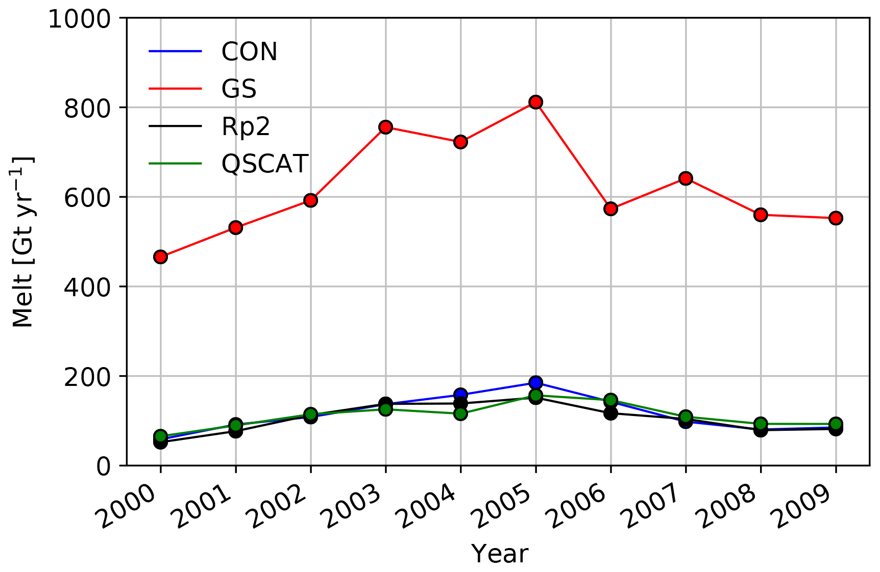
Figure 13Domain-integrated yearly-averaged melt for the AIS in Gt yr−1 measured by QSCAT and modeled in Rp2, GS and CON.
6.2 Melt comparison with an energy balance model
Figure 14 shows the cumulative melt at Neumayer station as calculated by the EBM of Jakobs et al. (2019), which is forced by meteorological data, and compares it with Rp2, GS and CON. Also for this location, GS predicts excessively high melt. This figure confirms that GS significantly overestimates melt and that tuning is necessary. CON initially underestimates melt, which is compensated for by increased meltwater production in the warm years of 2004, 2010 and 2014, ending closer to the cumulative melt of the EBM than Rp2.
In this study, we investigated the impact of a new snow albedo and radiative transfer scheme in the latest adaptation of the polar version of RACMO2.3 on the near-surface temperature, (sub)surface snow temperature, SMB, SEB, albedo and melt of the AIS. We tuned Rp3 by incrementally changing one parameter at a time, allowing us to investigate the sensitivity of the AIS to each change.
We have run Rp3 for the entire AIS on a 27 km grid forced at the boundaries by 3-hourly ERA5 data. Three experiments are run for the full period (1979–2018): Rp2, Rp3 with Greenland settings (GS) and the Rp3 control run (CON) that includes all tuning steps. The results are compared to in situ and remote sensing observations and to the previous model version Rp2. The other sensitivity experiments are done for 1979–1990 and include increasing the fresh snow SSA (FSG), reducing the fresh dry snow metamorphism (FSM) and lowering the refreezing grain size (RFG).
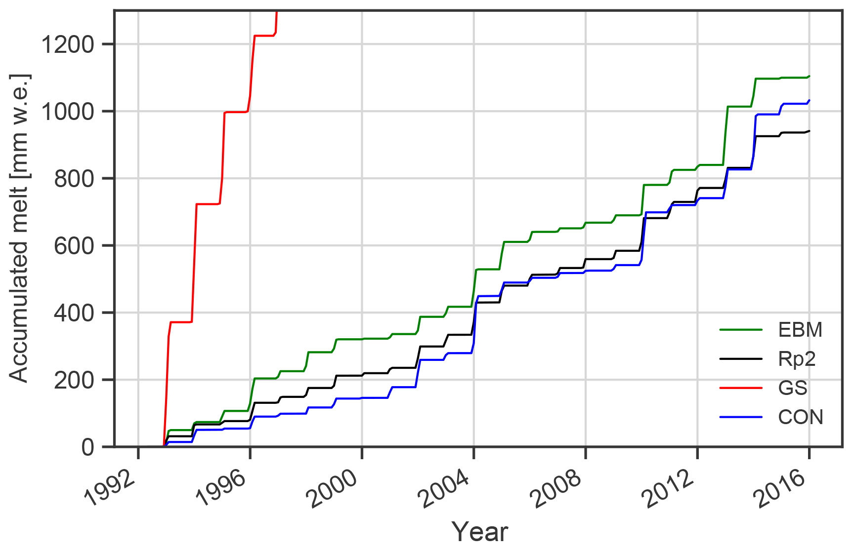
Figure 14Cumulative melt in mm w.e. at Neumayer calculated by the energy balance model (EBM) of Jakobs et al. (2019) and Rp2, GS and CON.
Compared to observations and Rp2, the 2 m temperature in the GS experiment is considerably higher. The sensitivity experiments show improvements, resulting in a lower bias with observations for CON. The reduction of the fresh dry snow metamorphism rate in the FSM experiment results in a lowering of the temperature. For some areas, however, the 2 m temperature is now too low. Yearly averaged, it is underestimated by up to 0.5 ∘C. This indicates, together with SSA observations, that the fresh dry snow metamorphism might have been reduced too strongly and that further improved results would likely be reached with a larger value for α of Eq. (1). More importantly, the results presented here highlight the necessity to correctly model snow conditions and that the current snow metamorphism scheme has to be improved or replaced. Nonetheless, subsurface temperatures of CON match well with observations at Dome C for the summer of 2007.
Analysis of the SEB shows that Rp3 exhibits, on average, some small (lower than 10 W m−2) persistent biases in the net radiative fluxes, which are caused by too transparent clouds and overestimated turbulent surface fluxes. This illustrates that there is still room for model development, especially in the turbulent fluxes. With the introduction of a new physically based albedo and radiative transfer scheme, more processes now impact the snow albedo. Radiation penetration and spectral shifts due to cloud cover and high SZA can lead to albedo differences up to −0.1 between CON and Rp2. Monthly-averaged, however, differences between these model versions are small.
The higher (subsurface) temperatures in GS lead to excessive melt around the margins and on the ice shelves, locally leading to runoff and a reduced SMB. Integrated over the AIS, melt in GS is 1 order of magnitude larger than observed by QSCAT and also considerably larger than measured at Neumayer station. In contrast, CON and Rp2 compare well with these observations. Melt is progressively reduced by all sensitivity experiments, especially in RFG and CON, showing the sensitivity of the AIS to the refreezing grain size and SLED. The difference between RFG and CON illustrates the importance of subsurface heating, which can warm the snowpack and enhance melt. Despite the low average melt flux in Antarctica, the impact of subsurface heating should not be neglected for a physical description of (sub)surface melt. It is clear that GS does not produce realistic meltwater fluxes and that the standard Greenland settings of Rp3 should not be used for the AIS. This is undesirable, as model settings should preferably not depend on location and/or tuning to local conditions, and shows that more research into this problem is needed.
In conclusion, introducing a new more physically based spectral snow albedo and radiative transfer scheme in the polar version of RACMO, which also allows for subsurface heating, improves, after tuning (as biases were partly compensated for in former RACMO versions), the subsurface snow temperatures in Antarctica. Incorrectly modeling snow conditions can lead to an order of magnitude melt overestimation and can significantly impact the climate and lower the SMB of the AIS. Furthermore, as is shown in the GS experiment, only a small lowering of summer albedo by, for example, global-warming-induced melting would lead to a very different near-surface summer climate in Antarctica.

Figure A1Summer mean monthly-averaged 2 m temperature (T2m) difference with Rp2 for (a) GS and (b) CON for 1985–2018, with positive values indicating a temperature increase with respect to Rp2.
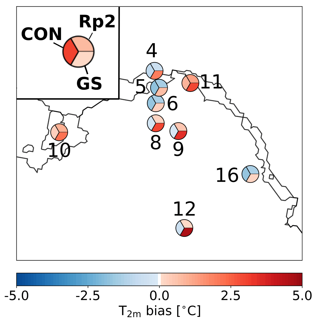
Figure A2Bias of monthly-averaged 2 m temperature (T2m) using AWS data of DML between 1997 and 2012. Each numbered circle chart represents an AWS station (locations shown in Fig. 2b) and is split into three parts: the upper right shows the bias of Rp2 with observations, the lower right GS and the left CON.
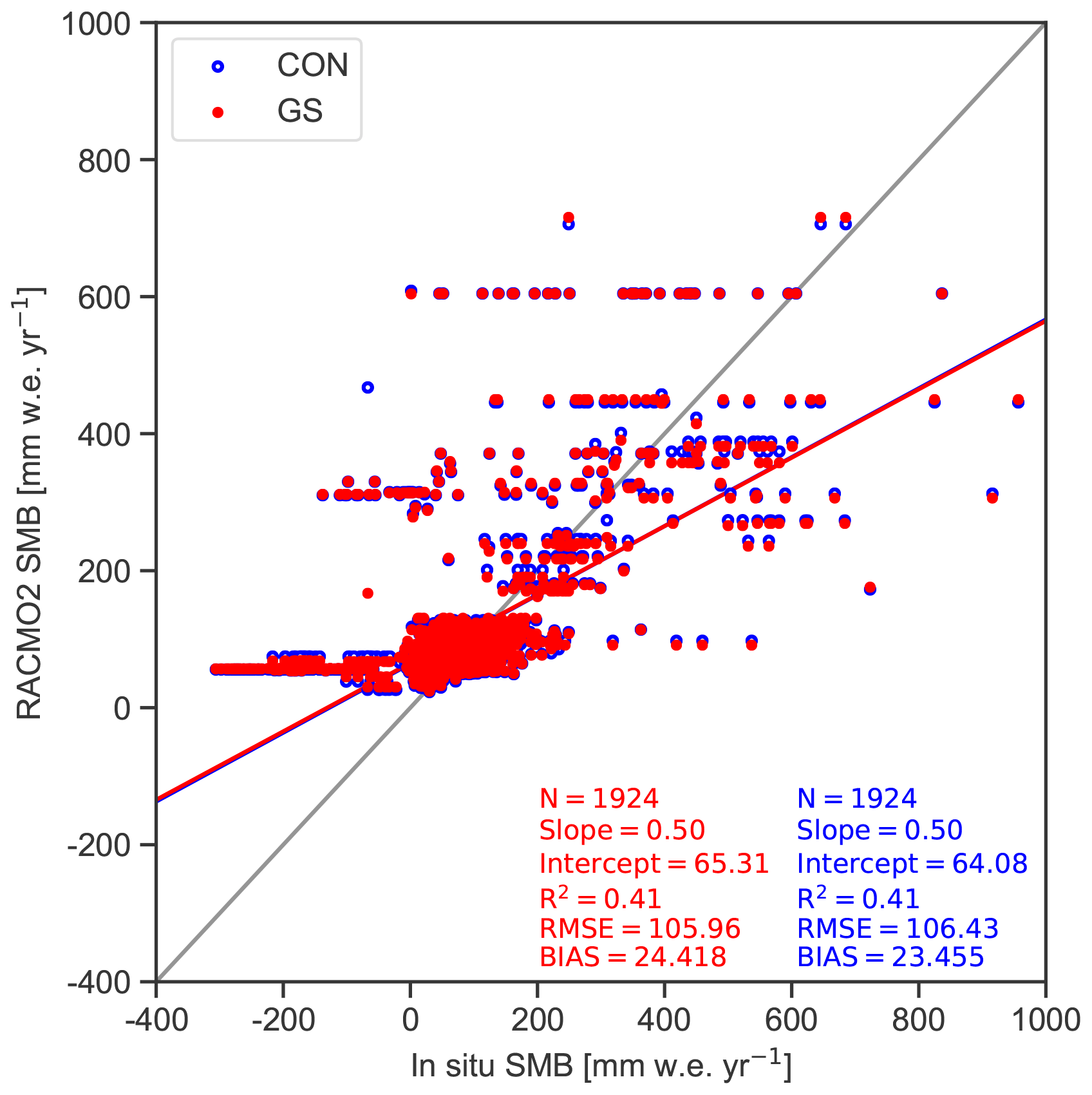
Figure A3Yearly-accumulated SMB in the EAIS in CON and GS compared to observations. The gray line is the one-on-one line, and the red and blue lines are linear regression of the data, with the number of observations (N), the slope, the intercept, the correlation coefficient (R2), the bias and root-mean-square error (RMSE). The intercept, bias and RMSE are in mm w.e. yr−1.
Table A1Domain-integrated yearly-averaged SMB and melt for the AIS in Gt yr−1 for Rp2 and the Rp3 sensitivity experiments for 1985–1990. For both variables, the difference with Rp2 in percentage is also shown.
Data are available at 27 km resolution for Antarctica for CON and GS (1979–2018) and FSG, FSM and RFG (1979–1990). Monthly-accumulated and monthly-averaged data for T2 m and SMB and their components are available for all Rp3 experiments. SEB components are available for GS and CON. The data can be found at https://doi.org/10.5281/zenodo.5512077 (Van Dalum et al., 2021a). Rp2 data are available from the authors. SMB observations can be found at https://doi.org/10.11888/Glacio.tpdc.271148 (Wang et al., 2021; Wang, 2021).
CTvD, WJvdB and MRvdB initiated this study and analyzed the results. CTvD led the writing of the manuscript, performed the simulations and implemented model changes. All authors contributed to the discussion on the manuscript.
At least one of the (co-)authors is a member of the editorial board of The Cryosphere. The peer-review process was guided by an independent editor, and the authors also have no other competing interests to declare.
Publisher’s note: Copernicus Publications remains neutral with regard to jurisdictional claims in published maps and institutional affiliations.
This publication was supported by PROTECT. This project has received funding from the European Union's Horizon 2020 research and innovation program under grant agreement no. 869304, PROTECT contribution number 30. We also acknowledge the ECMWF for archiving facilities and computational time on their supercomputers.
This research has been supported by Horizon 2020 (PROTECT grant no. 869304).
This paper was edited by Xavier Fettweis and reviewed by Cécile Agosta and two anonymous referees.
Agosta, C., Amory, C., Kittel, C., Orsi, A., Favier, V., Gallée, H., van den Broeke, M. R., Lenaerts, J. T. M., van Wessem, J. M., van de Berg, W. J., and Fettweis, X.: Estimation of the Antarctic surface mass balance using the regional climate model MAR (1979–2015) and identification of dominant processes, The Cryosphere, 13, 281–296, https://doi.org/10.5194/tc-13-281-2019, 2019. a
Bader, H.: Density of ice as a function of temperature and stress, https://hdl.handle.net/11681/11579, (last access: 18 June 2021), 1964. a
Bozkurt, D., Rondanelli, R., Marín, J. C., and Garreaud, R.: Foehn Event Triggered by an Atmospheric River Underlies Record-Setting Temperature Along Continental Antarctica, J. Geophys. Res.-Atmos., 123, 3871–3892, https://doi.org/10.1002/2017JD027796, 2018. a
Brucker, L., Picard, G., Arnaud, L., Barnola, J.-M., Schneebeli, M., Brunjail, H., Lefebvre, E., and Fily, M.: Modeling time series of microwave brightness temperature at Dome C, Antarctica, using vertically resolved snow temperature and microstructure measurements, J. Glaciol., 57, 171–182, https://doi.org/10.3189/002214311795306736, 2011. a, b
Cogley, J. G., Hock, R., Rasmussen, L., Arendt, A., Bauder, A., Braithwaite, R., Jansson, P., Kaser, G., Möller, M., Nicholson, L., and Zemp, M.: Glossary of glacier mass balance and related terms, IHP-VII technical documents in hydrology, UNESCO-International Hydrological Programme, 86, 965, 2011. a
Coléou, C. and Lesaffre, B.: Irreducible water saturation in snow: experimental results in a cold laboratory, Ann. Glaciol., 26, 64–68, https://doi.org/10.3189/1998AoG26-1-64-68, 1998. a
Dang, C., Brandt, R. E., and Warren, S. G.: Parameterizations for narrowband and broadband albedo of pure snow and snow containing mineral dust and black carbon, J. Geophys. Res.-Atmos., 120, 5446–5468, https://doi.org/10.1002/2014JD022646, 2015. a, b
Doherty, S. J., Warren, S. G., Grenfell, T. C., Clarke, A. D., and Brandt, R. E.: Light-absorbing impurities in Arctic snow, Atmos. Chem. Phys., 10, 11647–11680, https://doi.org/10.5194/acp-10-11647-2010, 2010. a
Domine, F., Taillandier, A.-S., and Simpson, W. R.: A parameterization of the specific surface area of seasonal snow for field use and for models of snowpack evolution, J. Geophys. Res.-Earth Surf., 112, F02031, https://doi.org/10.1029/2006JF000512, 2007. a
ECMWF: Part IV: Physical Processes, IFS Documentation, ECMWF, operational implementation 3 June 2008, ECMWF, 162 pp., https://doi.org/10.21957/8o7vwlbdr, 2009. a
Etourneau, J., Sgubin, G., Crosta, X., Swingedouw, D., Willmott, V., Barbara, L., Houssais, M.-N., Schouten, S., Damsté, J. S. S., Goosse, H., Escutia, C., Crespin, J., Massé, G., and Kim, J.-H.: Ocean temperature impact on ice shelf extent in the eastern Antarctic Peninsula, Nat. Commun., 10, 304, https://doi.org/10.1038/s41467-018-08195-6, 2019. a
Flanner, M. G. and Zender, C. S.: Linking snowpack microphysics and albedo evolution, J. Geophys. Res.-Atmos., 111, D12208, https://doi.org/10.1029/2005JD006834, 2006. a, b, c
Fretwell, P., Pritchard, H. D., Vaughan, D. G., Bamber, J. L., Barrand, N. E., Bell, R., Bianchi, C., Bingham, R. G., Blankenship, D. D., Casassa, G., Catania, G., Callens, D., Conway, H., Cook, A. J., Corr, H. F. J., Damaske, D., Damm, V., Ferraccioli, F., Forsberg, R., Fujita, S., Gim, Y., Gogineni, P., Griggs, J. A., Hindmarsh, R. C. A., Holmlund, P., Holt, J. W., Jacobel, R. W., Jenkins, A., Jokat, W., Jordan, T., King, E. C., Kohler, J., Krabill, W., Riger-Kusk, M., Langley, K. A., Leitchenkov, G., Leuschen, C., Luyendyk, B. P., Matsuoka, K., Mouginot, J., Nitsche, F. O., Nogi, Y., Nost, O. A., Popov, S. V., Rignot, E., Rippin, D. M., Rivera, A., Roberts, J., Ross, N., Siegert, M. J., Smith, A. M., Steinhage, D., Studinger, M., Sun, B., Tinto, B. K., Welch, B. C., Wilson, D., Young, D. A., Xiangbin, C., and Zirizzotti, A.: Bedmap2: improved ice bed, surface and thickness datasets for Antarctica, The Cryosphere, 7, 375–393, https://doi.org/10.5194/tc-7-375-2013, 2013. a
Gardner, A. S. and Sharp, M. J.: A review of snow and ice albedo and the development of a new physically based broadband albedo parameterization, J. Geophys. Res.-Earth Surf., 115, F01009, https://doi.org/10.1029/2009JF001444, 2010. a, b, c, d, e, f
Gelman Constantin, J., Ruiz, L., Villarosa, G., Outes, V., Bajano, F. N., He, C., Bajano, H., and Dawidowski, L.: Measurements and modeling of snow albedo at Alerce Glacier, Argentina: effects of volcanic ash, snow grain size, and cloudiness, The Cryosphere, 14, 4581–4601, https://doi.org/10.5194/tc-14-4581-2020, 2020. a
Grenfell, T. C. and Warren, S. G.: Representation of a nonspherical ice particle by a collection of independent spheres for scattering and absorption of radiation, J. Geophys. Res.-Atmos., 104, 31697–31709, https://doi.org/10.1029/1999JD900496, 1999. a
He, C. and Flanner, M.: Snow Albedo and Radiative Transfer: Theory, Modeling, and Parameterization, 67–133, Springer International Publishing, Cham, https://doi.org/10.1007/978-3-030-38696-2_3, 2020. a
Hersbach, H., Bell, B., Berrisford, P., Hirahara, S., Horányi, A., Muñoz-Sabater, J., Nicolas, J., Peubey, C., Radu, R., Schepers, D., Simmons, A., Soci, C., Abdalla, S., Abellan, X., Balsamo, G., Bechtold, P., Biavati, G., Bidlot, J., Bonavita, M., De Chiara, G., Dahlgren, P., Dee, D., Diamantakis, M., Dragani, R., Flemming, J., Forbes, R., Fuentes, M., Geer, A., Haimberger, L., Healy, S., Hogan, R. J., Hólm, E., Janisková, M., Keeley, S., Laloyaux, P., Lopez, P., Lupu, C., Radnoti, G., de Rosnay, P., Rozum, I., Vamborg, F., Villaume, S., and Thépaut, J.-N.: The ERA5 global reanalysis, Q. J. Roy. Meteorol. Soc., 146, 1999–2049, https://doi.org/10.1002/qj.3803, 2020. a
Jakobs, C. L., Reijmer, C. H., Kuipers Munneke, P., König-Langlo, G., and van den Broeke, M. R.: Quantifying the snowmelt–albedo feedback at Neumayer Station, East Antarctica, The Cryosphere, 13, 1473–1485, https://doi.org/10.5194/tc-13-1473-2019, 2019. a, b, c, d, e, f
Jiménez-Aquino, J. I. and Varela, J. R.: Two stream approximation to radiative transfer equation: An alternative method of solution, Rev. Mex. Fis., 51, 82–86, 2005. a
Kokhanovsky, A. A.: Light scattering Media Optics: Problems and Solutions, Springer, Berlin, Germany, ISBN: 3540211845, 299 pp., 2004. a
Kuipers Munneke, P., Van den Broeke, M. R., Lenaerts, J. T. M., Flanner, M. G., Gardner, A. S., and Van de Berg, W. J.: A new albedo parameterization for use in climate models over the Antarctic ice sheet, J. Geophys. Res.-Atmos., 116, D05114, https://doi.org/10.1029/2010JD015113, 2011. a, b
Kuipers Munneke, P., Picard, G., van den Broeke, M. R., Lenaerts, J. T. M., and van Meijgaard, E.: Insignificant change in Antarctic snowmelt volume since 1979, Geophys. Res. Lett., 39, L01501, https://doi.org/10.1029/2011GL050207, 2012. a
Kuipers Munneke, P., Luckman, A. J., Bevan, S. L., Smeets, C. J. P. P., Gilbert, E., van den Broeke, M. R., Wang, W., Zender, C., Hubbard, B., Ashmore, D., Orr, A., King, J. C., and Kulessa, B.: Intense Winter Surface Melt on an Antarctic Ice Shelf, Geophys. Res. Lett., 45, 7615–7623, https://doi.org/10.1029/2018GL077899, 2018. a
Legagneux, L., Taillandier, A.-S., and Domine, F.: Grain growth theories and the isothermal evolution of the specific surface area of snow, J. Appl. Phys., 95, 6175–6184, https://doi.org/10.1063/1.1710718, 2004. a, b
Lenaerts, J. T. M., Lhermitte, S., Drews, R., Ligtenberg, S. R. M., Berger, S., Helm, V., Smeets, C. J. P. P., Broeke, M. R. V. d., Van de Berg, W. J., Van Meijgaard, E., Eijkelboom, M., Eisen, O., and Pattyn, F.: Meltwater produced by wind–albedo interaction stored in an East Antarctic ice shelf, Nat. Clim. Change, 7, 58–62, https://doi.org/10.1038/nclimate3180, 2017. a, b
Libois, Q., Picard, G., France, J. L., Arnaud, L., Dumont, M., Carmagnola, C. M., and King, M. D.: Influence of grain shape on light penetration in snow, The Cryosphere, 7, 1803–1818, https://doi.org/10.5194/tc-7-1803-2013, 2013. a
Libois, Q., Picard, G., Arnaud, L., Dumont, M., Lafaysse, M., Morin, S., and Lefebvre, E.: Summertime evolution of snow specific surface area close to the surface on the Antarctic Plateau, The Cryosphere, 9, 2383–2398, https://doi.org/10.5194/tc-9-2383-2015, 2015. a
Ligtenberg, S., Lenaerts, J., Van Den Broeke, M., and Scambos, T.: On the formation of blue ice on Byrd Glacier, Antarctica, J. Glaciol., 60, 41–50, https://doi.org/10.3189/2014JoG13J116, 2014. a
Ligtenberg, S. R. M., Kuipers Munneke, P., Noël, B. P. Y., and van den Broeke, M. R.: Brief communication: Improved simulation of the present-day Greenland firn layer (1960–2016), The Cryosphere, 12, 1643–1649, https://doi.org/10.5194/tc-12-1643-2018, 2018. a
Martin, D. F., Cornford, S. L., and Payne, A. J.: Millennial-Scale Vulnerability of the Antarctic Ice Sheet to Regional Ice Shelf Collapse, Geophys. Res. Lett., 46, 1467–1475, https://doi.org/10.1029/2018GL081229, 2019. a
Meyer, H., Katurji, M., Appelhans, T., Müller, M., Nauss, T., Roudier, P., and Zawar-Reza, P.: Mapping Daily Air Temperature for Antarctica Based on MODIS LST, Remote Sens., 8, 732, https://doi.org/10.3390/rs8090732, 2016. a
Mottram, R., Hansen, N., Kittel, C., van Wessem, J. M., Agosta, C., Amory, C., Boberg, F., van de Berg, W. J., Fettweis, X., Gossart, A., van Lipzig, N. P. M., van Meijgaard, E., Orr, A., Phillips, T., Webster, S., Simonsen, S. B., and Souverijns, N.: What is the surface mass balance of Antarctica? An intercomparison of regional climate model estimates, The Cryosphere, 15, 3751–3784, https://doi.org/10.5194/tc-15-3751-2021, 2021. a
Noël, B., van de Berg, W. J., van Wessem, J. M., van Meijgaard, E., van As, D., Lenaerts, J. T. M., Lhermitte, S., Kuipers Munneke, P., Smeets, C. J. P. P., van Ulft, L. H., van de Wal, R. S. W., and van den Broeke, M. R.: Modelling the climate and surface mass balance of polar ice sheets using RACMO2 – Part 1: Greenland (1958–2016), The Cryosphere, 12, 811–831, https://doi.org/10.5194/tc-12-811-2018, 2018. a, b
Picard, G., Domine, F., Krinner, G., Arnaud, L., and Lefebvre, E.: Inhibition of the positive snow-albedo feedback by precipitation in interior Antarctica, Nat. Clim. Change, 2, 795–798, https://doi.org/10.1038/nclimate1590, 2012. a
Picard, G., Libois, Q., Arnaud, L., Verin, G., and Dumont, M.: Development and calibration of an automatic spectral albedometer to estimate near-surface snow SSA time series, The Cryosphere, 10, 1297–1316, https://doi.org/10.5194/tc-10-1297-2016, 2016. a, b, c, d
Picard, G., Arnaud, L., Caneill, R., Lefebvre, E., and Lamare, M.: Observation of the process of snow accumulation on the Antarctic Plateau by time lapse laser scanning, The Cryosphere, 13, 1983–1999, https://doi.org/10.5194/tc-13-1983-2019, 2019. a, b
Rignot, E., Mouginot, J., Scheuchl, B., van den Broeke, M., van Wessem, M. J., and Morlighem, M.: Four decades of Antarctic Ice Sheet mass balance from 1979–2017, P. Natl. Acad. Sci. USA, 116, 1095–1103, https://doi.org/10.1073/pnas.1812883116, 2019. a
Shepherd, A., Ivins, E., Rignot, E., Smith, B., van den Broeke, M., Velicogna, I., Whitehouse, P., Briggs, K., Joughin, I., Krinner, G., Nowicki, S., Payne, T., Scambos, T., Schlegel, N., A, G., Agosta, C., Ahlstrøm, A., Babonis, G., Barletta, V., Blazquez, A., Bonin, J., Csatho, B., Cullather, R., Felikson, D., Fettweis, X., Forsberg, R., Gallee, H., Gardner, A., Gilbert, L., Groh, A., Gunter, B., Hanna, E., Harig, C., Helm, V., Horvath, A., Horwath, M., Khan, S., Kjeldsen, K. K., Konrad, H., Langen, P., Lecavalier, B., Loomis, B., Luthcke, S., McMillan, M., Melini, D., Mernild, S., Mohajerani, Y., Moore, P., Mouginot, J., Moyano, G., Muir, A., Nagler, T., Nield, G., Nilsson, J., Noel, B., Otosaka, I., Pattle, M. E., Peltier, W. R., Pie, N., Rietbroek, R., Rott, H., Sandberg-Sørensen, L., Sasgen, I., Save, H., Scheuchl, B., Schrama, E., Schröder, L., Seo, K.-W., Simonsen, S., Slater, T., Spada, G., Sutterley, T., Talpe, M., Tarasov, L., van de Berg, W. J., van der Wal, W., van Wessem, M., Vishwakarma, B. D., Wiese, D., and Wouters, B.: Mass balance of the Antarctic Ice Sheet from 1992 to 2017, Nature, 558, 219–222, https://doi.org/10.1038/s41586-018-0179-y, 2018. a
Solomon, S., Schmeltekopf, A. L., and Sanders, R. W.: On the interpretation of zenith sky absorption measurements, J. Geophys. Res.-Atmos., 92, 8311–8319, https://doi.org/10.1029/JD092iD07p08311, 1987. a
Sommerfeld, R. A. and LaChapelle, E.: The Classification of Snow Metamorphism, J. Glaciol., 9, 3–18, https://doi.org/10.3189/S0022143000026757, 1970. a
Trusel, L. D., Frey, K. E., Das, S. B., Munneke, P. K., and van den Broeke, M. R.: Satellite-based estimates of Antarctic surface meltwater fluxes, Geophys. Res. Lett., 40, 6148–6153, https://doi.org/10.1002/2013GL058138, 2013. a
Trusel, L. D., Frey, K. E., Das, S. B., Karnauskas, K. B., Kuipers Munneke, P., van Meijgaard, E., and van den Broeke, M. R.: Divergent trajectories of Antarctic surface melt under two twenty-first-century climate scenarios, Nat. Geosci., 8, 927–932, https://doi.org/10.1038/ngeo2563, 2015. a
Undén, P., Rontu, L., Jarvinen, H., Lynch, P., Calvo Sánchez, F., Cats, G., Cuxart, J., Eerola, K., Fortelius, C., García-Moya, J., and Jones, C.: HIRLAM-5 Scientific Documentation, http://www.hirlam.org/index.php/hirlam-documentation/cat_view/114-model-and-system-documentation/131-hirlam-documentation?limit=5&order=date&dir=ASC&start=10, (last access: 18 June 2021), 2002. a
van Dalum, C. T., van de Berg, W. J., Libois, Q., Picard, G., and van den Broeke, M. R.: A module to convert spectral to narrowband snow albedo for use in climate models: SNOWBAL v1.2, Geosci. Model Dev., 12, 5157–5175, https://doi.org/10.5194/gmd-12-5157-2019, 2019. a, b
van Dalum, C. T., van de Berg, W. J., Lhermitte, S., and van den Broeke, M. R.: Evaluation of a new snow albedo scheme for the Greenland ice sheet in the Regional Atmospheric Climate Model (RACMO2), The Cryosphere, 14, 3645–3662, https://doi.org/10.5194/tc-14-3645-2020, 2020. a, b, c, d, e, f
Van Dalum, C., Van de Berg, W., and Van den Broeke, M.: RACMO2.3p3 monthly SMB, SEB and t2m data for Antarctica (1979–2018), Zenodo [data set], https://doi.org/10.5281/zenodo.5512077, 2021a. a
van Dalum, C. T., van de Berg, W. J., and van den Broeke, M. R.: Impact of updated radiative transfer scheme in snow and ice in RACMO2.3p3 on the surface mass and energy budget of the Greenland ice sheet, The Cryosphere, 15, 1823–1844, https://doi.org/10.5194/tc-15-1823-2021, 2021b. a, b, c, d, e, f, g, h, i, j
van de Berg, W. J., van Meijgaard, E., and van Ulft, L. H.: The added value of high resolution in estimating the surface mass balance in southern Greenland, The Cryosphere, 14, 1809–1827, https://doi.org/10.5194/tc-14-1809-2020, 2020. a
van den Broeke, M. R., Enderlin, E. M., Howat, I. M., Kuipers Munneke, P., Noël, B. P. Y., van de Berg, W. J., van Meijgaard, E., and Wouters, B.: On the recent contribution of the Greenland ice sheet to sea level change, The Cryosphere, 10, 1933–1946, https://doi.org/10.5194/tc-10-1933-2016, 2016. a, b
van Wessem, J. M., Ligtenberg, S. R. M., Reijmer, C. H., van de Berg, W. J., van den Broeke, M. R., Barrand, N. E., Thomas, E. R., Turner, J., Wuite, J., Scambos, T. A., and van Meijgaard, E.: The modelled surface mass balance of the Antarctic Peninsula at 5.5 km horizontal resolution, The Cryosphere, 10, 271–285, https://doi.org/10.5194/tc-10-271-2016, 2016. a, b
van Wessem, J. M., van de Berg, W. J., Noël, B. P. Y., van Meijgaard, E., Amory, C., Birnbaum, G., Jakobs, C. L., Krüger, K., Lenaerts, J. T. M., Lhermitte, S., Ligtenberg, S. R. M., Medley, B., Reijmer, C. H., van Tricht, K., Trusel, L. D., van Ulft, L. H., Wouters, B., Wuite, J., and van den Broeke, M. R.: Modelling the climate and surface mass balance of polar ice sheets using RACMO2 – Part 2: Antarctica (1979–2016), The Cryosphere, 12, 1479–1498, https://doi.org/10.5194/tc-12-1479-2018, 2018. a, b, c
Wang, Y.: A comprehensive dataset of surface mass balance field observations over the Antarctic Ice Sheet, National Tibetan Plateau Data Center [data set], https://doi.org/10.11888/Glacio.tpdc.271148, 2021. a, b
Wang, Y., Ding, M., Reijmer, C. H., Smeets, P. C. J. P., Hou, S., and Xiao, C.: The AntSMB dataset: a comprehensive compilation of surface mass balance field observations over the Antarctic Ice Sheet, Earth Syst. Sci. Data, 13, 3057–3074, https://doi.org/10.5194/essd-13-3057-2021, 2021. a, b
Warren, S. G.: Optical properties of ice and snow, Philos. T. R. Soc. A, 377, 20180161, https://doi.org/10.1098/rsta.2018.0161, 2019. a, b
Warren, S. G. and Clarke, A. D.: Soot in the atmosphere and snow surface of Antarctica, J. Geophys. Res.-Atmos., 95, 1811–1816, https://doi.org/10.1029/JD095iD02p01811, 1990. a
WMO: New record for Antarctic continent reported, WMO, https://public.wmo.int/en/media/news/new-record-antarctic-continent-reported, (last access: 18 June 2021), 2020. a
- Abstract
- Introduction
- Methods and data
- Results: temperature
- Specific surface area comparison
- Surface energy balance and albedo analysis
- Surface mass balance and melt
- Summary and conclusions
- Appendix A
- Data availability
- Author contributions
- Competing interests
- Disclaimer
- Acknowledgements
- Financial support
- Review statement
- References