the Creative Commons Attribution 4.0 License.
the Creative Commons Attribution 4.0 License.
 | 16 Mar 2022
A local model of snow–firn dynamics and application to the Colle Gnifetti site
Carlo De Michele
The regulating role of glaciers in catchment run-off is of fundamental importance in sustaining people living in low-lying areas. The reduction in glacierized areas under the effect of climate change disrupts the distribution and amount of run-off, threatening water supply, agriculture and hydropower. The prediction of these changes requires models that integrate hydrological, nivological and glaciological processes. In this work we propose a local model that combines the nivological and glaciological scales. The model describes the formation and evolution of the snowpack and the firn below it, under the influence of temperature, wind speed and precipitation. The model has been implemented in two versions: (1) a multi-layer one that considers separately each firn layer and (2) a single-layer one that models firn and underlying glacier ice as a single layer. The model was applied at the site of Colle Gnifetti (Monte Rosa massif, 4400–4550 ). We obtained an average reduction in annual snow accumulation due to wind erosion of 2×10³ to be compared with a mean annual precipitation of about 2.7×10³ . The conserved accumulation is made up mainly of snow deposited between April and September, when temperatures above the melting point are also observed. End-of-year snow density, instead, increased an average of 65 kg m−3 when the contribution of wind to snow compaction was added. Observations show a high spatial and interannual variability in the characteristics of snow and firn at the site and a correlation of net balance with radiation and the number of melt layers. The computation of snowmelt in the model as a sole function of air temperature may therefore be one of the reasons for the observed mismatch between model and observations.
- Article
(12113 KB) - Full-text XML
- BibTeX
- EndNote


Glacier ice covers almost 16×106 km2 of the Earth's surface, of which it is estimated that only 3 % is retained by the mountains outside the polar regions (Benn and Evans, 2010). Despite this small percentage, the amount of water stored in mountain glaciers plays a key role in sustaining people living in low-lying areas (Adhikary, 1993), influencing run-off on a wide range of temporal and spatial scales (Jansson et al., 2003; Huss et al., 2010). Storing water coming from precipitation in winter and delaying the time in which it reaches the river network, mountain glaciers sustain streamflow in hotter and drier periods when precipitation is lacking and when it is most needed for agriculture and as drinking water (Fountain and Tangborn, 1985; Hagg et al., 2007).
Jost et al. (2012) studied a Canadian river basin, covered for only 5 % by glaciers, and they found that ice melt contributes up to 25 % to streamflow in August, up to 35 % to streamflow in September, and between 3 % and 9 % to total streamflow.
In high mountain river basins of the northern Tian Shan (central Asia), with areas of glaciation higher than 30 %–40 %, glacier melt contribution is 18 %–28 % of annual run-off but it can increase to 40 %–70 % during summer (Aizen et al., 1996).
The reduction in glacier volume observed over the past 150 years (Vaughan et al., 2013; Hock et al., 2019) will result in a change in the present distribution and amount of water storage and release, with implications for all aspects of watershed management (Hock et al., 2005) and with consequently high economic impacts (Huss et al., 2010). The prediction of these changes is therefore fundamental in order to assess and reduce their impacts, optimizing consequently the management of water resources. To accomplish this task, models that integrate hydrological, nivological and glaciological components and that consider a variable glacier extension and the transient response of glaciers to climate change are required (Luo et al., 2013).
Despite their importance, fully integrated glacio-hydrological catchment models are not common in the literature (Wortmann et al., 2019). Some examples of glacio-hydrological models are provided by the works of Huss et al. (2010), Naz et al. (2014), Seibert et al. (2018) and Wortmann et al. (2019).
Wortmann et al. (2019) grouped the main problems of glacio-hydrological models into two categories: integration and scale. With integration problems they refer to the simplified or absent description of the remaining catchment hydrology in models that describe glacier processes in detail. The decrease in the fraction of ice-covered areas requires a proper description of both components, even in basins that are currently highly glacierized. Another aspect is the integration of nivological and glaciological components: a joint simulation of glacier mass balance and snow accumulation and melt is required in order to avoid inconsistencies (Jost et al., 2012; Naz et al., 2014). The problems of scale arise from the different resolutions required by glacial, nivological and hydrological processes. Physically based models that consider all glacier processes (mass balance, subglacial drainage and ice flow dynamics) are often too computationally expensive to be used in a combined glacio-hydrological model that considers the entire catchment. In addition, they are characterized by a complexity higher than the one of many semi-distributed hydrological models. It is therefore necessary to develop glacier models with a degree of complexity similar to the one of hydrological models but that are still able to reproduce important processes (Seibert et al., 2018).
In the present work, we give our contribution proposing a local model that follows the transformation of snow into firn and glacier ice under the influence of meteorological variables (temperature, precipitation and wind speed). Existing firn densification models are, in general, forced by snow characteristics. In this sense, the presented model allows us to move the boundary of the firn densification models from surface accumulation and density to hourly meteorological series. When we do not assume stationarity in the climate, in fact, this is required to properly capture the effects of climate changes.
The core of the model was derived from mass balance, momentum balance and rheological equations, governing the evolution of snowpack and firn (depth and density of snow and firn, depth of water and refrozen meltwater and rain inside the snowpack). The calculations of the terms in the resulting equations were then approached looking at methods already used in the literature; for example, snowmelt mass flux was computed with a temperature-index approach and the run-off from the snowpack with a flow matrix approach. We present two versions of the model: (1) a version (multi-layer) that considers separately each firn layer and (2) a version (single-layer) that models firn and underlying glacier ice as a single layer. The latter consists of only six equations, and it is therefore more suitable for a possible application to a hydrological model. The former consists of four equations for the snowpack plus two equations for each firn layer. Providing a profile of density with depth, it captures better the influence of meteorological variables on snow and firn characteristics. Besides, it allows a better validation of the snow–firn model. The equations that describe the snowpack are derived from the work of De Michele et al. (2013) and later Avanzi et al. (2015), modified in order to take into account the contribution of wind erosion and the transformation of snow into firn. To model the firn component, both the densification model of Arnaud et al. (2000) and the one of Herron and Langway (1980) were implemented. In order to test the model, a high-altitude site, Colle Gnifetti, belonging to the Monte Rosa massif, was chosen.
The paper is organized as follows: we present the model in Sect. 2, illustrate the case study in Sect. 3, give the results in Sect. 4 and discuss them in Sect. 5. The conclusions are given in Sect. 6.
In this section, firstly the snowpack model, proposed by De Michele et al. (2013) and later modified by Avanzi et al. (2015) with the addition of the contribution of wind to snow transport, is illustrated and secondly the model with the integration of snow and firn processes is presented.
2.1 Snow model
The snowpack is modelled, according to De Michele et al. (2013) and Avanzi et al. (2015), as a mixture of dry and wet constituents. The solid deformable skeleton that consists of both snow grains and pores has a total volume VS, unit area, height hS, mass MS and density ρS. The liquid water inside the pores has a volume VW, unit area, height hW, mass MW and constant density . The refrozen meltwater and rain inside the pores has a volume VMF with unit area, height hMF, mass MMF and constant density . It is also possible to define the bulk snow density ρ, snow water equivalent SWE and volumetric liquid water content θW as , and , where h is the height of the snowpack equal to (Avanzi et al., 2015) with ϕ being the porosity and 〈〉 denoting the Macaulay brackets that provide zero when the argument is negative and its value when it is positive. The height h and hS always coincide except at the end of the snowpack existence when the liquid part and the solid part due to refreezing become predominant (i.e. ). In this case, h>hS because a layer of water and/or ice forms on top of the deformable skeleton.
The model solves the mass balance for the dry and liquid mass of the snowpack and the momentum balance and rheological equation for the solid deformable skeleton, resulting in four ordinary differential equations (ODEs) with the variables hS, hW, hMF and ρS. The mass fluxes considered are (1) solid precipitation events, snowmelt and wind erosion for the dry-snow mass; (2) rain events, snowmelt, melt–freeze inside the snowpack and run-off for the liquid mass; and (3) melt–freeze for the mass of ice. The dry-snow density is obtained considering (1) the compaction of snow due to compaction not driven by wind, (2) the increase in the densification rate due to drifting snow settlement and (3) densification due to the addition of new mass. The following system is thus obtained (see Appendix Sects. A1–A2 for the derivation of the system and a detailed description of the terms in the equations):
In Eq. (1a), ρNS is the density of fresh snow (kg m−3), s is the solid precipitation rate (m h−1), a is a calibration parameter (), TA and Tτ are the air temperature and the threshold temperature for melting (∘C), I is equal to with k equal to 0.01 m if TA≥Tτ and zero otherwise (Avanzi et al., 2015), and Q is the mass of snow eroded by wind (). In Eq. (1b), r is the liquid precipitation rate (m h−1), e is a calibration parameter, I* is equal to if TA<Tτ and to if TA>Tτ (Avanzi et al., 2015), (DeWalle and Rango, 2008), and KW is the intrinsic permeability of water in snow (m2). In Eq. (1d), , A1=0.0013 m−1, , (Liston et al., 2007), U is the wind speed contribution (m s−1), and TS is the average snow temperature (∘C) obtained assuming thermal equilibrium between the constituents and a bilinear profile of temperature through depth (see De Michele et al., 2013, for further details).
With respect to the model by De Michele et al. (2013) and Avanzi et al. (2015), the version presented in this work includes the contribution of wind erosion to mass balance and effect of wind on densification. This is important when the model is applied to high-altitude sites: Haeberli and Alean (1985), in fact, suggested that a major part of the decrease in accumulation with altitude in the Alps that occurs above about 3500 may be due to wind effects.
In analogy with solid transport, snow is mobilized only when wind velocity at the surface exceeds a given threshold that depends on physical properties of the surface snowpack (Li and Pomeroy, 1997). Once transport begins, snow can travel in two main modes: saltation and suspension (Déry and Taylor, 1996; Pomeroy et al., 1997). The total snow transport Q is computed by the model with the following assumptions: (1) only snow erosion occurs, and no deposition of snow eroded in other positions is present; (2) measured wind speed is always referred to a 10 m height – i.e. the height of the snow on the ground is neglected; and (3) wind cannot erode snow that has experienced a temperature greater than 0 ∘C for the presence of ice crusts or wet layers, following Vionnet et al. (2018). These last two assumptions allow us to compute the series of total snow transport Q decoupled from the snow model since knowledge of snow height is not required. In order to implement the routine, we followed, with some modifications, Lehning et al. (2000), where a model of snowdrift was added to the one-dimensional snow model SNOWPACK (further details about the implementation of the routine are reported in Appendix Sect. A1).
2.2 Model of snow–firn dynamics
We propose here two versions of the snow–firn model. The first version (single-layer) models firn and underlying glacier ice as a single layer (Fig. 1, left panel). The resulting output is an average density and the total column height. The second version (multi-layer) considers separately each firn layer (Fig. 1, right panel), and it allows us to distinguish between layers of firn and glacier ice. The discretized profile of density with depth can be obtained from this second implementation. The snow layer is, instead, treated as a single layer in both versions.
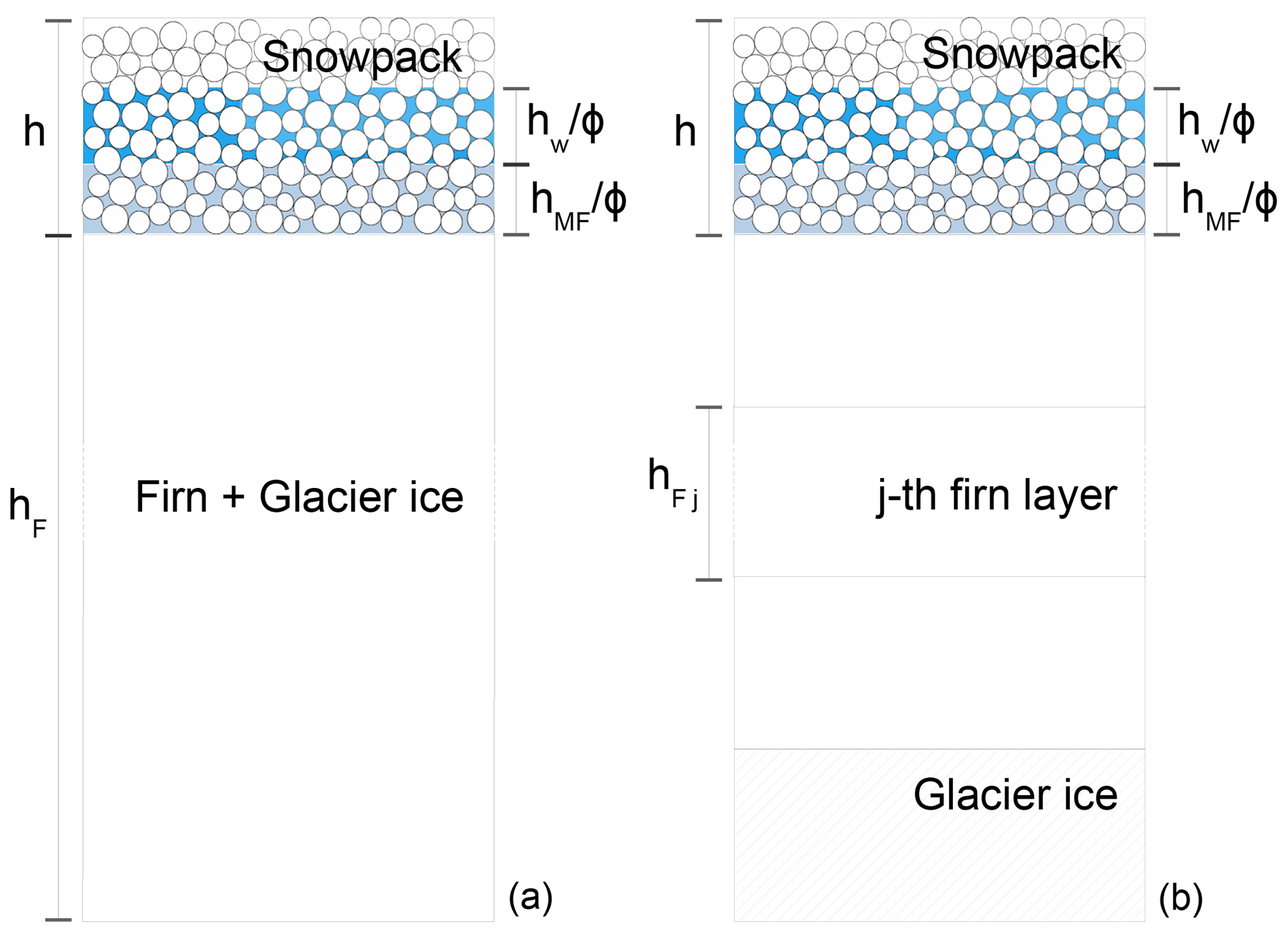
Figure 1A column of snow, firn and ice as modelled by the single-layer (a) and multi-layer (b) version of the snow–firn model.
In the model we neglected the amount of water percolation inside firn. The presence of water inside firn varies greatly depending on the type of glacier. At high altitudes, where maximum temperatures are rarely positive, the effects of percolation due to melting are limited (Smiraglia et al., 2000); at the cold site of Colle Gnifetti, where the model was applied, percolation occurs only in the few centimetres below the surface and does not involve previous-year layers (Alean et al., 1983). If needed, the structure of the model allows us to easily implement additional processes.
In order to separate snow from firn, we refer to firn's original definition, according to which firn is snow that has survived one melt season (Cuffey and Paterson, 2010).
2.2.1 One-layer modelling of firn
The model is composed of two layers: the snowpack (see Sect. 2.1) and the column of firn below it. The firn is modelled as a single impermeable layer of volume VF, unit area, height hF, mass MF and density ρF (Fig. 1, left panel).
The model consists of six ODEs: the four equations of the snow model and in addition the mass balance and momentum balance of firn. The mass variation in firn is obtained considering firn melt, the effects of precipitation on firn and the transformation of snow into firn at the end of each hydrological year. The firn densification rate is obtained considering densification due to overburden stress and densification due to addition of new mass. The resulting system is thus as follows (see Appendix A for the derivation of the system and a detailed description of the terms in the equations):
The last terms in Eqs. (2a)–(2c) move, at the end of each melt season, the remaining snowpack (if present) in the firn layer; ti is the time instant at the end of hydrological year i and δ(.) is the Dirac delta function. In Eq. (2d), IF is equal to , with k specified above if TA≥Tτ and equal to zero otherwise. In Eq. (2f), is the densification of firn due to compaction (see Sect. 2.4). Equations (2a)–(2f) are impulsive differential equations (see e.g. Bainov and Simeonov, 1993, for mathematical details). This type of differential equation involving the impulse effect is used to describe the evolution of many physical phenomena that have a sudden change in their states such as mechanical systems with impact; biological systems such as heartbeats and blood flows; and population dynamics.
2.3 Multi-layer modelling of firn
Firn is modelled as a multi-layer column where each layer j has volume VFj, unit area, height hFj, mass MFj and density ρFj.
The equations of the model change as follows:
where j goes from 2 to the total number of firn layers. Firn layers that reach the ice density or whose height goes to zero are removed from the model.
2.4 Firn densification
The densification of firn due to compaction is usually subdivided into three stages: (1) a first stage dominated by the settling of grains that allows us to reach densities of up to about 550 kg m−3, (2) a second stage dominated by sintering that extends up to the close-off density (i.e. the density at which pores become isolated) of about 830 kg m−3 and (3) a last stage that ends when ice density is reached in which further densification is driven by the compression of the bubbles of air (Cuffey and Paterson, 2010). This last stage is in turn subdivided into two phases, depending on if the pores are cylindrical or spherical. Different models of firn densification are available in the literature (see Lundin et al., 2017, for a review). Here we implemented the model of Arnaud et al. (2000) with some of the modifications proposed by Bréant et al. (2017) (we will refer to it with the abbreviation AR) and the model of Herron and Langway (1980) (we will refer to it with the abbreviation HL). Other models could also be implemented. Both HL and AR were developed for polar sites. The HL model was derived using ice cores with a mean annual firn temperature between −57 and −15 ∘C and a mean annual accumulation between 0.022×10³ and 0.5×10³ , while the AR model was derived from cores with a mean annual firn temperature between −57 and −19 ∘C and a mean annual accumulation between 0.022×10³ and 1.1×10³ . In the model of AR, densification equations are based on grain sliding and creep deformations, even though they maintain empirical parameters. The model of HL consists of empirical equations tuned with ice cores, based on the assumption that a proportionality is present between the variation in density and the variation in stress due to new accumulation. Besides, the model of AR represents stresses explicitly, while in HL the load is parametrized through annual surface accumulation.
The model of HL was already applied to non-polar ice cores by Huss (2013), where the model was recalibrated in order to match depth–density profiles of temperate and polythermal firn. In the presented application, the parameters were not recalibrated, despite the fact that the study site is an alpine site. This was motivated by the low mean annual firn temperature (MAFT) and low surface accumulation observed at Colle Gnifetti that resemble conditions of some polar sites.
In AR all three stages of firn densification are modelled. Equations are as follows:
In the first stage (), P is the overburden pressure (Pa) and in which RG is the gas constant, Q1 an activation energy equal to , TF the average temperature of firn (∘C), and γ′ a parameter whose value is set in order to have a continuous densification rate between the first and second stage (estimated in Sect. 4.2). DD is the relative surface density, and D0 is the relative density at the transition between the first stage and the second stage. In the second stage (), with , ac is the average contact area, Z is the number of particle contacts (see Appendix Sect. A3 for the expression of ac and Z) and Q2 is an activation energy. The value of Q2 was set to 60×103 J mol−1, as in the model of Arnaud et al. (2000), since it is the typical activation energy associated with self-diffusion of ice. However, at higher temperature (i.e. higher than −10 ∘C) a higher activation energy may be required to best fit density profiles with firn densification models (Cuffey and Paterson, 2010; Arthern et al., 2010; Jacka and Jun, 1994). A discussion of the thermal variation in the creep parameter and the impact of the different sintering mechanisms on it can be found in Bréant et al. (2017). Lastly, in the third stage (), Pb is the pressure inside the bubbles equal to with Dc and Pc the relative density and pressure at the transition between the second and third stage. In the single-layer version, the overburden pressure P was computed as the overburden of the snowpack layer plus half of the firn layer. In the multi-layer version, we computed the overburden for each layer of firn as the overburden of the snowpack plus the overburden of all the firn layers above plus the overburden of half the firn layer considered.
In HL only the first and second densification stages are modelled. The equations are as follows:
where , and ω is the annual snow accumulation (). In HL the transition density between the first and second stage is fixed and equal to 550 kg m−3. In order to run the model of HL in a dynamic way, for each year we computed the annual accumulation averaging the ones modelled between the year of deposition of the firn layer and the year before the one considered, following Stevens et al. (2020).
Steady-state firn densification models are not applied to the superficial snow where the metamorphism is more complex and significantly influenced by air temperature. The original model of Arnaud et al. (2000), for example, was used only for depths higher than 2 m. In this case, we applied them only to densities higher than a density ρD, which represents the average snow density. For firn densities lower than ρD, the densification equation of snow was adopted although neglecting wind contribution. In this way, the transition between the two equations is driven by density rather than associated with the end of a water year. This is important, for example, when consistent fresh snow falls over the snowpack at the end of the hydrological year.
2.4.1 Temperature profile
The energetic description of the volume was simplified assuming the constituents were in thermal equilibrium and assuming a bilinear profile of temperature through depth. Temperature was assumed to vary linearly from the surface temperature T0 to the MAFT at the depth zM at which seasonal variation in temperature is negligible. Below zM, temperature was kept constant and equal to MAFT. In cold glaciers the value of MAFT is close to the mean annual air temperature (MAAT) when meltwater percolation is limited (Suter et al., 2001) while in temperate glaciers it is equal to the melting temperature (Cuffey and Paterson, 2010). Surface temperature was fixed equal to TA if TA<0 ∘C and zero otherwise. Huss (2013) has already assumed a bilinear profile of temperature in order to study temperate firn densification, fixing zM to 5 m since it is the typical penetration of winter air temperature. The temperature profile was then used to compute the average snow and firn temperatures that influence snow and firn densification.
2.5 Numerical model
The model was solved using the forward Euler method with a constant step size, Δt, of 1 h. To also compute the last terms in Eqs. (1d), (2f) and (3g) when hS, hF and are zero, these terms were calculated, following De Michele et al. (2013), as , and . Regarding the vertical discretization, the firn component of the multi-layer version of the model was discretized modelling one layer for each hydrological year.
In the following section we will present the study area (Sect. 3.1), the data collection and handling (Sect. 3.2–3.3), and finally the calibration and site-specific parameters (Sect. 3.4–3.5).
3.1 Study area
The site of Colle Gnifetti (CG) is part of the summit ranges of the Monte Rosa massif, Swiss–Italian Alps. It is the uppermost part of the accumulation area of the Grenzgletscher (Border Glacier), and it forms a saddle that lies between the Signalkuppe (4554 ) and Zumsteinspitze (4563 ) at an altitude of 4400–4550 (Lüthi and Funk, 2000) (Fig. 2). The glacier at Colle Gnifetti has a thickness of between 60 and 120 m and a MAFT of −14 ∘C (Wagenbach et al., 2012). The regime is that of a high-altitude site, i.e. nearly persistent sub-zero air temperature, a high precipitation total and high wind speed (Suter et al., 2001). A mean annual precipitation of 2.7×10³ with an interannual variability of (Mariani et al., 2014) was estimated for the period 1961–1993 from a core extracted at the upper Grenzgletscher (Eichler et al., 2000).
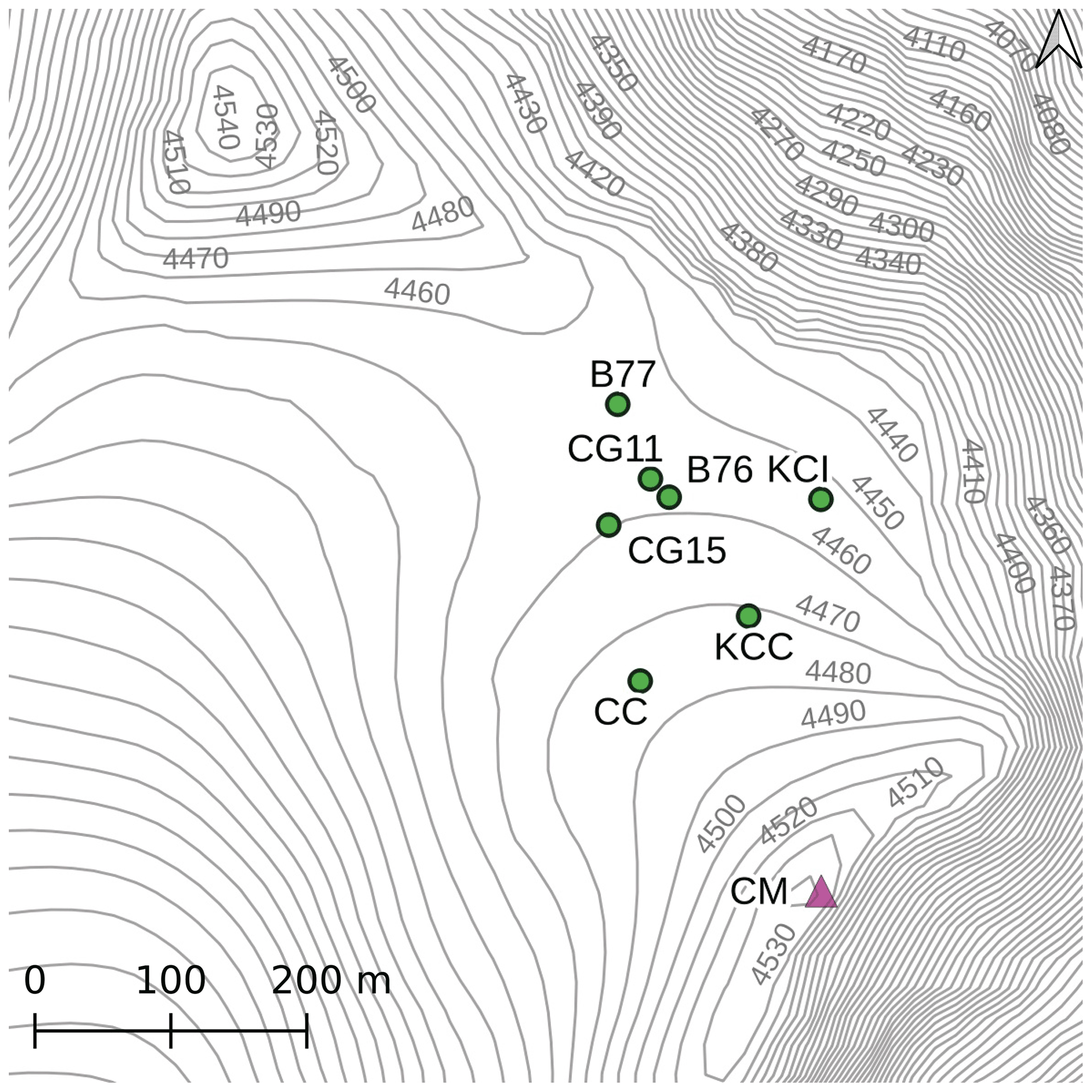
Figure 2The site of Colle Gnifetti and the location of the ice cores considered in the present work. CG03 and CG15 ice core share the same location therefore CG03 is not shown. The position of Capanna Regina Margherita (CM) is also shown.
Even though the site is characterized by high precipitation totals, accumulation in the saddle is considerably lower and highly variable over the glacier surface due to wind erosion, with values ranging from about 0.15×10³ to 1.2×10³ depending on the wind exposure (Alean et al., 1983; Lüthi and Funk, 2000; Licciulli et al., 2020). Alean et al. (1983) measured the accumulation at CG between 17 August 1980 and 23 July 1982 with a network of 30 stakes. For the period between 14 August 1981 and 23 July 1982 the mass balance was negative at all the stakes due to wind erosion, while the net accumulation of the hydrological year 1980–1981 varied between and with the highest values on south-facing slopes. This occurs because the enhanced melting and refreezing cause the formation of wet layers and ice crusts and because higher temperatures are associated with faster densification, and both these aspects reduce the possibility of wind eroding snow. This also results in the fact that almost all the snow that survives the melt season comes from summer events (Bohleber et al., 2018; Schöner et al., 2002).
3.2 Data collection
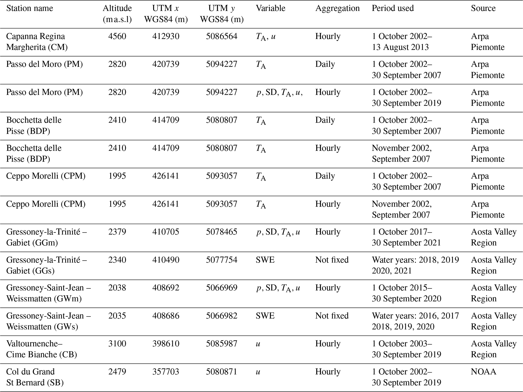
The stations whose data were used in this study are presented in Fig. 3, and they are summarized in Table 1. Hourly data of air temperature and wind speed at Capanna Regina Margherita (CM, Margherita Hut in English) were used as input for the model; hourly data at Passo del Moro (PM, Monte Moro Pass in English) to reconstruct precipitation at CM; and hourly and daily air temperature data at Macugnaga Pecetto (MP), Passo del Moro, Bocchetta delle Pisse (BDP) and Ceppo Morelli (CPM) to infill missing temperature data at Capanna Regina Margherita. Hourly wind speed data at Valtournenche–Cime Bianche (CB) and Col du Grand St Bernard (SB, Great St Bernard Pass in English) were used to infill missing wind speed data at CM. Hourly data at the meteorological stations of Gressoney-Saint-Jean – Weissmatten (GWm) and Gressoney-la-Trinité – Gabiet (GGm) and snow water equivalent data (GWs and GGs) were used to calibrate and validate the parameters a and e of the snow model. Snow water equivalent is measured by the Aosta Valley Region during winter both at fixed locations and at itinerant sites. For GGs, 4 years of measurements was available with on average 24 data points for each winter. For GWs, 5 years was available with on average 8 data points for each winter.
The station of Capanna Regina Margherita, whose data were used to run the snow–firn model, was installed in 2002 by the Piedmont Region at the Regina Margherita Hut as part of a project that aimed to study the interaction between synoptic flow and orography. With its 4560 m of altitude, it can be considered the highest meteorological station in Europe, and its wind speed series can be considered representative of the synoptic conditions (Martorina et al., 2003). Due to its recent installation, the use of these data limits the length of the simulation and the number of cores with which our results can be compared. Nevertheless, we believe that, given the peculiar characteristics of the station, the use of these data may give added value to this study.
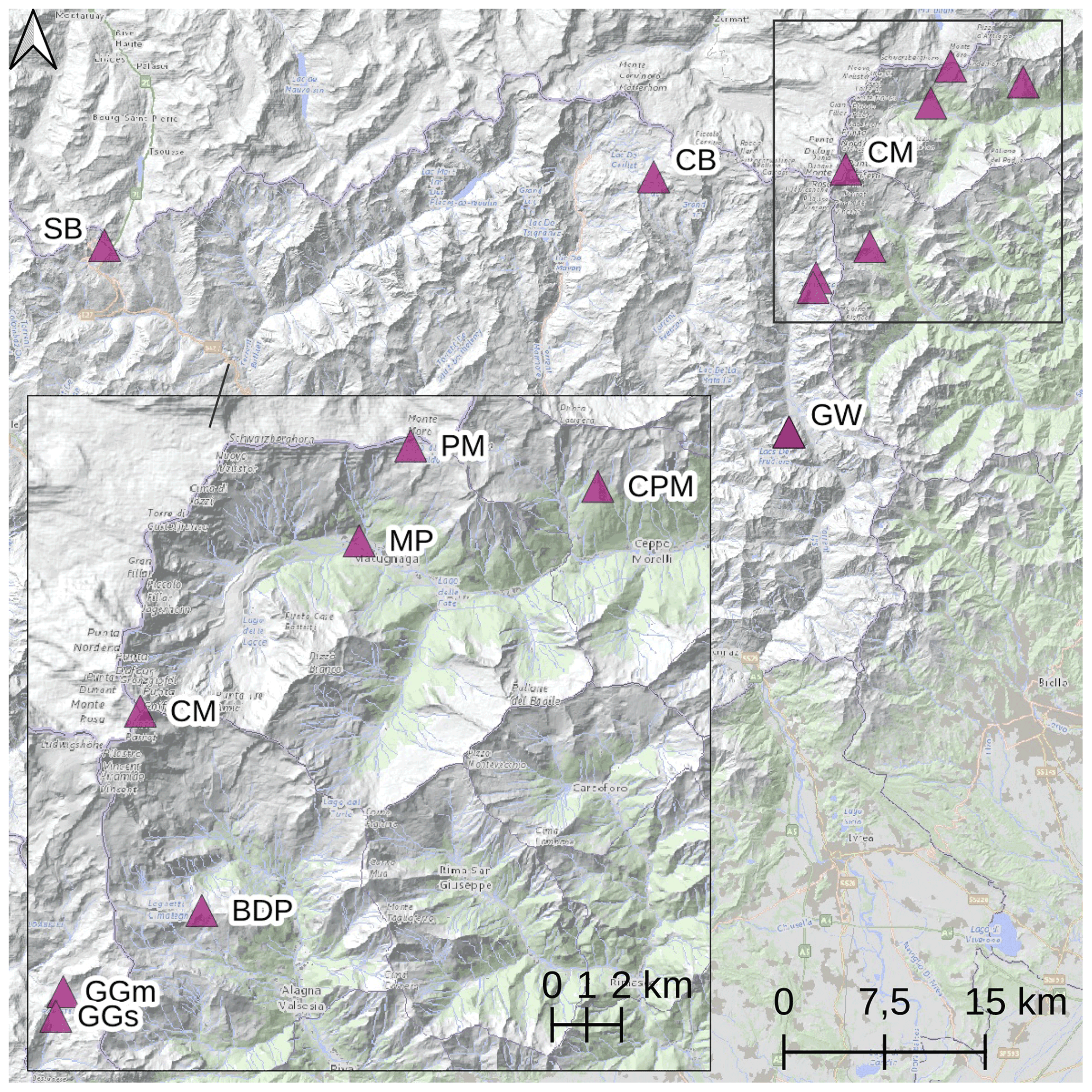
Figure 3Location of the meteorological stations used: Capanna Regina Margherita (CM), Macugnaga Pecetto (MP), Ceppo Morelli (CPM), Passo del Moro (PM), Bocchetta delle Pisse (BDP), Col du Grand St Bernard (SB), Valtournenche–Cime Bianche (CB), Gressoney-la-Trinité – Gabiet (GGm and GGs) and Gressoney-Saint-Jean – Weissmatten (GWm and GWs). The location of the meteorological station at Weissmatten and the location of snow measurements are only a few metres apart, so only one point is reported (identified with GW). In the bottom left panel a zoom over some stations is included. All stations belong to Arpa Piemonte with the exclusion of CB, GGm, GGs, GWm and GWs, which belong to the Aosta Valley Region, and SB, which belongs to the National Oceanic and Atmospheric Administration (NOAA). Source of the basemap: Arpa Piemonte geoportal.
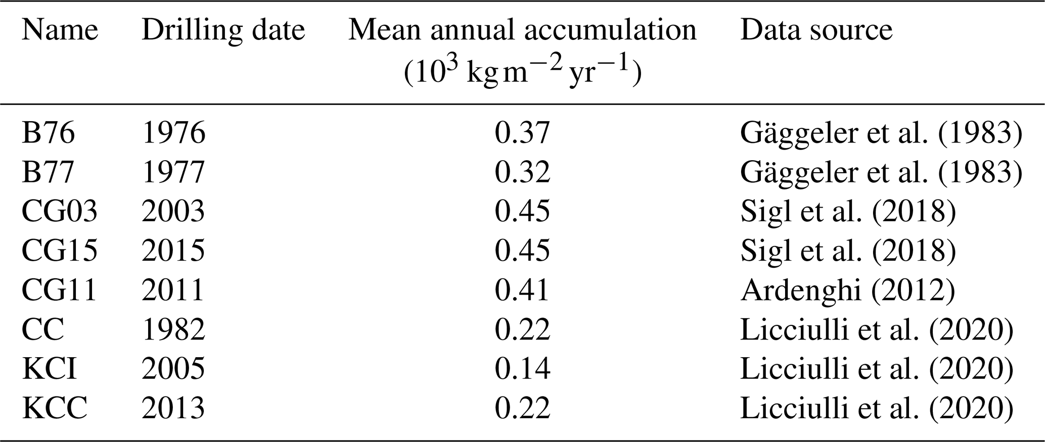
In Table 2 ice core data are reported (Fig. 2). Available data consist of some or all of the following information: depth in metres, depth in metres of water equivalent, density and dating. We recall that the first three variables are related, so one of them can be computed given the other two.
Table 1Meteorological data employed in the case study (p stands for precipitation, SD for snow depth, TA for air temperature, u for average wind speed and s for fresh snow). Hydrological years are identified by the last year; e.g. 2009 is hydrological year 2008–2009. With the term hydrological year we refer to the period from 1 October to 30 September of the next year.
3.3 Data handling
The model requires as input a continuous series of air temperature, precipitation and wind speed.
Following the comparison presented by Henn et al. (2013), to fill missing hourly temperature data at Capanna Margherita, the MicroMet preprocessor (Liston and Elder, 2006) was adopted for gaps smaller than 24 h and a long-term lapse rate approach with five stations (CM, MP, CPM, PM, BDP) was adopted for longer gaps. MicroMet is a meteorological model that includes a data-fill procedure adopted here. The method distinguishes between three conditions: (1) for 1 h gaps the missing information is replaced with the average of the previous and next measurement; (2) for 2–24 h gaps each missing value is replaced with the average of the values recorded the next and previous day at the same hour; (3) for longer gaps an auto-regressive integrated moving average (ARIMA) model is used (Hyndman and Athanasopoulos, 2021). Here, for the third condition, the long-term lapse rate approach was used, as specified above. In the period 1 October 2002–13 August 2013, 0.37 % of hourly temperature data were missing. After the MicroMet procedure 0.23 % remained missing and were substituted with a long-term lapse rate approach.
Wind speed data measured at CM are characterized by repeated zero values that are not observed in nearby stations and that are probably due to the freezing of the anemometer. In the period 1 October 2002–13 August 2013 nearly 30 % of the wind speed data at CM were equal to zero, while 1.3 % were missing. By comparison, in the same period, there were 2 % zero values in SB series. These zero values were therefore considered missing. To fill missing wind speed data at CM, the MicroMet procedure was used for gaps smaller than 24 h. For gaps longer than 24 h, data were replaced using measurements at CB or, if wind speed data were also missing at CB, with data measured at SB. In both series, zero wind speed values recorded for more than 4 consecutive hours were set as missing. In order to take into account the different characteristics of the sites, we first computed for each of the three stations the mean and standard deviation for each hour of the year, and we removed this from the data. Missing data at CM were first replaced with the corresponding residual value measured at CB (or SB), and then the final value was obtained using the mean and standard deviation estimated at CM. Reconstructed negative wind speed values at CM were set to zero. Missing wind speed data at CM were set to zero if they were zero at CB (or SB).
The precipitation series at CM was reconstructed using hourly data measured at PM. The station was chosen due to it being in the vicinity of CM and its altitude of 2820 . Using the formula proposed by Alpert (1986) and considering a bell-shaped mountain, we estimated for the Monte Rosa massif an altitude of maximum precipitation of zm=2547 m. The altitude of maximum precipitation is away from the crest as is typical of large mountains (Roe, 2005). We therefore expect to have similar precipitation totals at CM and PM. The precipitation series measured at PM needs to be integrated with snow depth data due to the under-catch of solid precipitation by the pluviometer or does not catch solid precipitation events in winter. In order to reconstruct the total precipitation series, we followed the routine presented by Avanzi et al. (2014). Solid precipitation is obtained looking at the positive variations in snow depth data, while rainfall is given by the difference, if positive, between total precipitation and solid precipitation. Positive variations in snow depth, however, may also be recorded when strong temperature variations occur, thus introducing false events. Unlike Avanzi et al. (2014), we approached this problem smoothing the snow depth series with a moving average whose window size was calibrated running the snow model at PM and looking for the best match between simulations and observations. Even though PM has an altitude higher than the estimated altitude of maximum precipitation, we obtained a mean annual precipitation of about 2×10³ for the period 2002–2019, lower than the one estimated at CG by Mariani et al. (2014). We suppose this may be due to wind erosion events; the procedure implemented by Avanzi et al. (2014), in fact, may compensate for snow depth variations due to wind erosion decreasing the estimated solid precipitation. We therefore increased the resulting hourly solid precipitation with a constant factor in order to match the observed mean annual accumulation at CG of 2.7×10³ . The total precipitation series was then divided between solid and liquid precipitation using a threshold of 1 ∘C since this is the value generally found in Europe (Jennings et al., 2018).
3.4 Calibration of model's parameters
The model requires the calibration of three parameters, namely a and e in Eqs. (1a)–(1c) and γ′ in Eq. (4).
The parameters a and e were calibrated running the snow model, with the addition of the wind module, at Gressoney-Saint-Jean – Weissmatten, with an hourly time step from 1 October 2015 to 30 September 2020. Input series were processed as reported for PM in Sect. 3.3. The parameter a governs the amount of snowmelt and consequently snow height and the relative amount of snow and ice inside the snowpack, thus influencing snow water equivalent and density. On the contrary, the parameter e influences only the relative amount of snow and ice inside the snowpack and does not contribute to snow height. The calibration problem is therefore a multi-objective one, since we could optimize the error in both snow height and density or SWE. We decided to move from a multi-objective to a single-objective optimization problem, aggregating the NSE (Nash–Sutcliffe efficiency) between observed and simulated snow depth data and the NSE between observed and simulated snow water equivalent data. We calculated the error metrics considering together all the available years but computing the measure only in the periods with snow depth higher than zero, and we aggregated them, giving a weight of 0.7 to the first and 0.3 to the second. In this way we took into account the higher uncertainty in SWE data due to the shorter sample length and the non-coincidence between the location of the meteorological station and the snow measurements. The optimum parameters were then estimated for different moving-average windows, used to process solid precipitation input data, with the use of a population-evolution-based algorithm, namely SCE-UA (Shuffled Complex Evolution – University of Arizona) (Duan et al., 1992, 1993). We thus obtained a pair of a and e values for each window, and we selected the one maximizing the objective function. The validation was performed applying the model with the selected set of parameters at Gressoney-la-Trinité – Gabiet for the period 1 October 2017–30 September 2021.
The parameter γ′, which governs the firn densification rate in AR, was chosen in order to have a continuous densification rate between the first and second stage of densification. For each of the available ice cores, with the exception of CG11, we computed the parameter γ′ running AR in a steady-state condition (Bader, 1954) using the mean accumulation reported in Table 2. In addition, the parameters of the firn densification model chosen may need calibration if applied to sites significantly different from the polar ones.
3.5 Site-specific parameters
In order to apply AR we use D0=0.56 (Bréant et al., 2017), (Lüthi and Funk, 2000) and Dc=0.9 since the precise value is not known at CG (Lüthi and Funk, 2000). Two different firn temperatures, and , that cover the observed ice temperatures at CG (Lüthi and Funk, 2000) were tested together with different surface densities, chosen looking at values already used in the literature at CG. We selected three values: ρD=300 kg m−3, ρD=360 kg m−3 and ρD=410 kg m−3, the values already assumed by Licciulli et al. (2020) and Lüthi and Funk (2000). The model of AR was run with a slight modification. We used the first-stage densification equation up to a relative density of 0.6, but we kept D0=0.56 in the second-stage densification equation. The latter, in fact, cannot be applied for D=D0, and it gives densification rates tending to infinity for values tending to D0. The other site-specific parameters of the snow–firn model that require specification are zM, set to 5 m (Haeberli and Funk, 1991), and the grain radius R, which influences the threshold wind speed. It is defined as , where SSA is the specific surface area in m2 kg−1. SSA was computed adopting the parametrization of Domine et al. (2007) for recent snow: .
4.1 Parameters' estimation
We obtained a value of the parameters a and e of 2.94×10⁻⁴ m h−1 ∘C−1 and 0.164, respectively. The combined NSE in calibration is 0.82, with a NSE of 0.84 and 0.78 for snow depth and snow water equivalent data, respectively. In validation, the combined NSE and the NSE values for snow depth and snow water equivalent are 0.77, 0.84 and 0.61, respectively. We also computed the RMSE and mean bias error (MBE) in validation, which are equal to 0.126×10³ and 0.0116×10³ for snow water equivalent and 0.26 and 0.0672 m for snow depth. Avanzi et al. (2014) estimated the parameter a for a selection of 40 sites with altitudes between 91 and 3389 within the SNOTEL (Snow Telemetry) network, a network of automated stations located in mountain basins of the western USA and operated by the Natural Resources Conservation Service (NRCS). They obtained median values of a of between 1×10⁻⁴ and 6×10⁻⁴ m h−1 ∘C−1. Regarding the parameter e, values of 0.2 and 0.25 were estimated by Avanzi et al. (2015) for two sites in Japan.
4.2 Steady-state firn densification
The depth–density profiles obtained using the model of AR and HL in a steady-state condition are reported in Fig. 4 for a surface density ρD=360 kg m−3. Both HL and AR have very good performances when applied to the KCC ice core. The worst performances occur for CG03 with an underestimation of the densification rate for all depths. For the remaining ice cores the models of AR and HL have a good fit up to depths of about 20–30 m, but they underestimate the densification rate below it. The profiles show in general a better performance of HL. We recall that the model of HL was derived also considering cores with MAFT and accumulation close to the ones of CG, while AR was optimized for cores with lower MAFT.
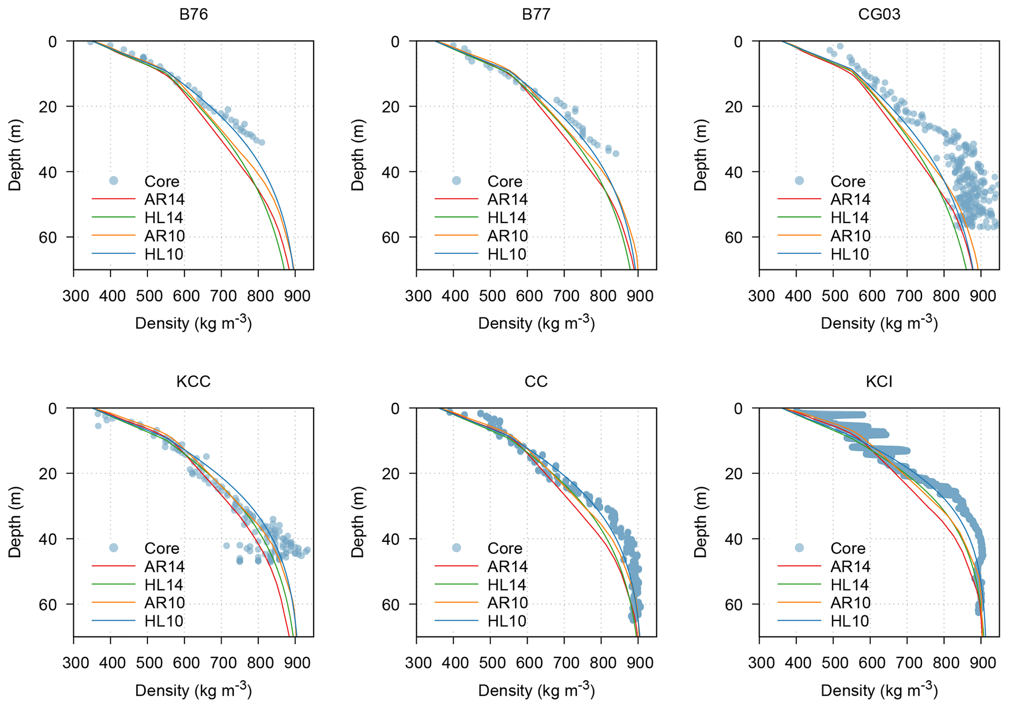
Figure 4Observed and modelled depth–density profiles. Modelled profiles are obtained running Arnaud et al. (2000) (AR) and Herron and Langway (1980) (HL) in a steady-state condition. The numbers 14 and 10 stand for a mean annual firn temperature of −14 and −10 ∘C, respectively.
4.3 Snow accumulation
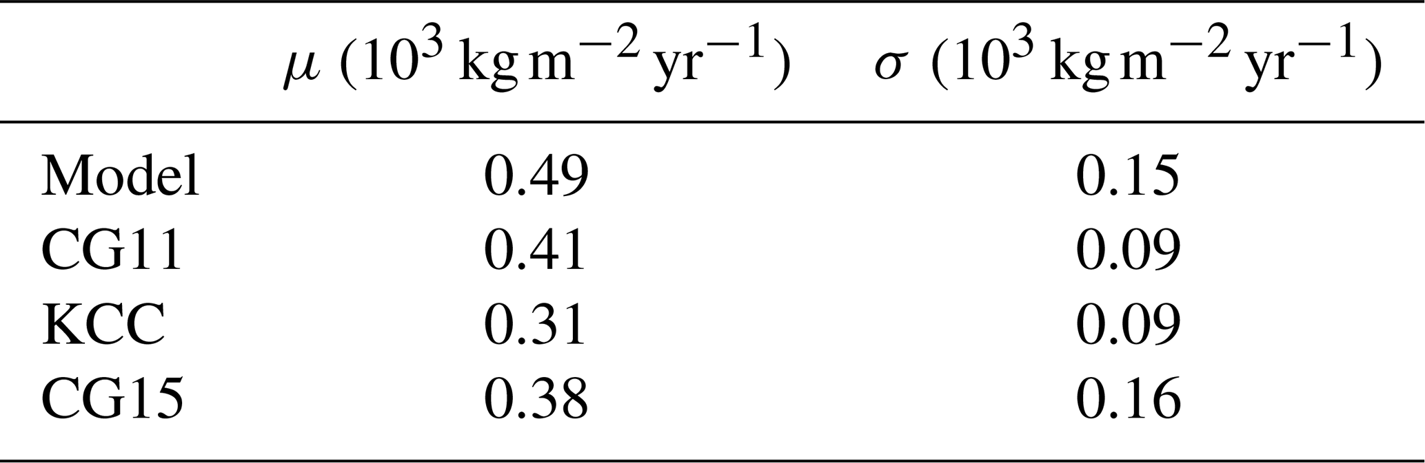
The annual accumulation obtained from the snow–firn model is reported in Fig. 5, along with the values retrieved from the three available ice cores, the average value of the observations and its 95 % confidence interval. The RMSE between the model and the average of the observations is equal to 0.22×10³ , and the modelled and observed average annual accumulation and standard deviation are reported in Table 3.

Figure 5Annual accumulation modelled and retrieved from three ice cores. The average of the annual accumulations from ice cores and its 95 % confidence interval are also reported.
Table 3Modelled and observed mean (μ) and standard deviation (σ) of the accumulation rate for the period 2003–2010.
In order to better understand the characteristics of the accumulation at CG, the monthly box plots of snow transport; solid precipitation; number of hours with , which in the model correspond to hours with melting; and monthly contribution to annual accumulation, computed for each month as 100 × (solid precipitation − eroded snow) solid precipitation, are provided in Fig. 6. Since snow is moved into firn at the end of September and wind is not allowed to erode firn, the fraction of conserved snow of September may be overestimated and the snow transport of October underestimated. We can see that annual accumulation is composed of snow deposited mainly between April and September, with June the month that on average contributes the most. The months in which solid precipitation is conserved are also the months in which temperature goes above the melting point; winter snow, instead, is completely removed.
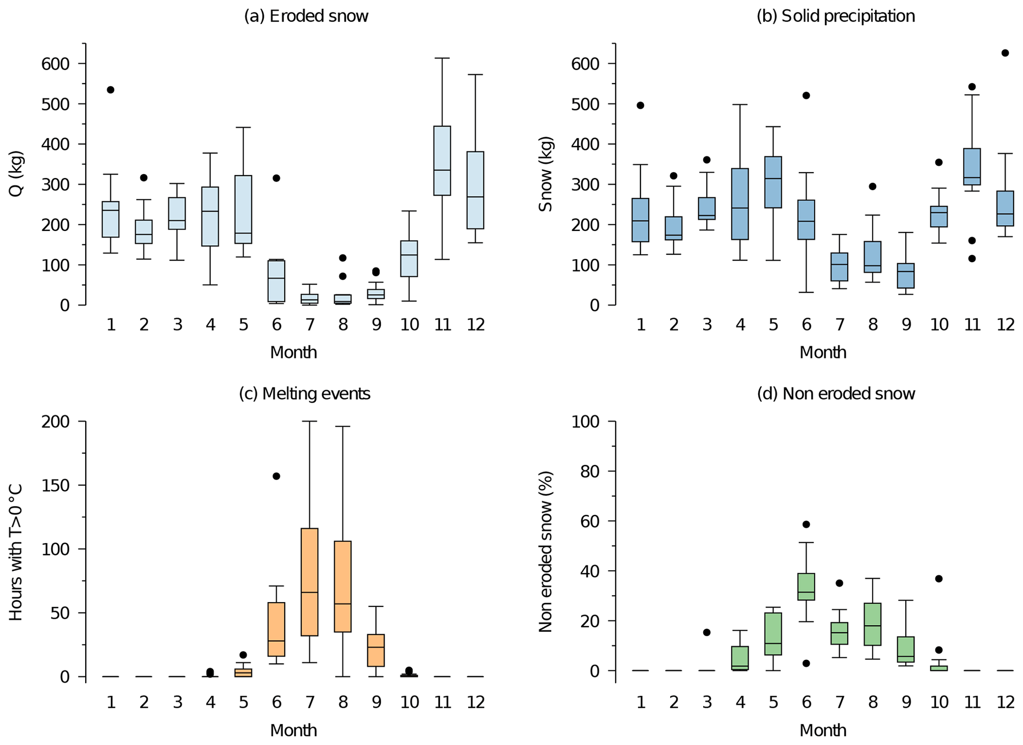
Figure 6Box plots of monthly eroded snow (a), monthly solid precipitation (b), monthly number of hours with above-zero temperatures (c) and monthly fraction of conserved solid precipitation (d), obtained for the period 1 October 2002–30 September 2015. The horizontal bar inside the box is drawn at the median, and the upper and lower ends of the box are drawn at the upper and lower quartile, respectively. The vertical lines, called whiskers, extend up to the most distant point that has a value within 1.5 times the interquartile range. The points outside these limits are drawn individually with dots.
4.4 Firn density
4.4.1 One-layer model version
The modelled firn density was compared with the density estimated from KCC and CG15 ice cores. With the one-layer version, we obtain one average value of firn density for each run of the model. We therefore run the model multiple times, fixing the end year of the simulation to the date of the core drilling and anticipating at each run the starting date of 1 year. For each run, the corresponding observed firn density was obtained averaging the density profile of the ice core associated with the same range of years. The results obtained implementing both AR and HL are reported in Fig. 7. For KCC we fixed the MAFT to −14 ∘C, while for CG15 we fixed it to −10 ∘C, looking for the best performance in Fig. 4.
Regarding firn density, we have contrasting results depending on the core and the densification model adopted. Both model versions overestimate KCC density with a better performance when AR is implemented; on the contrary we obtained an underestimation of CG15 average density, with a better performance when HL is implemented. In all the combinations, however, we observed a reduction in the error when more firn layers are averaged.
Moving to firn depth, the model nearly always predicts higher depths, with more significant differences for the KCC ice core.
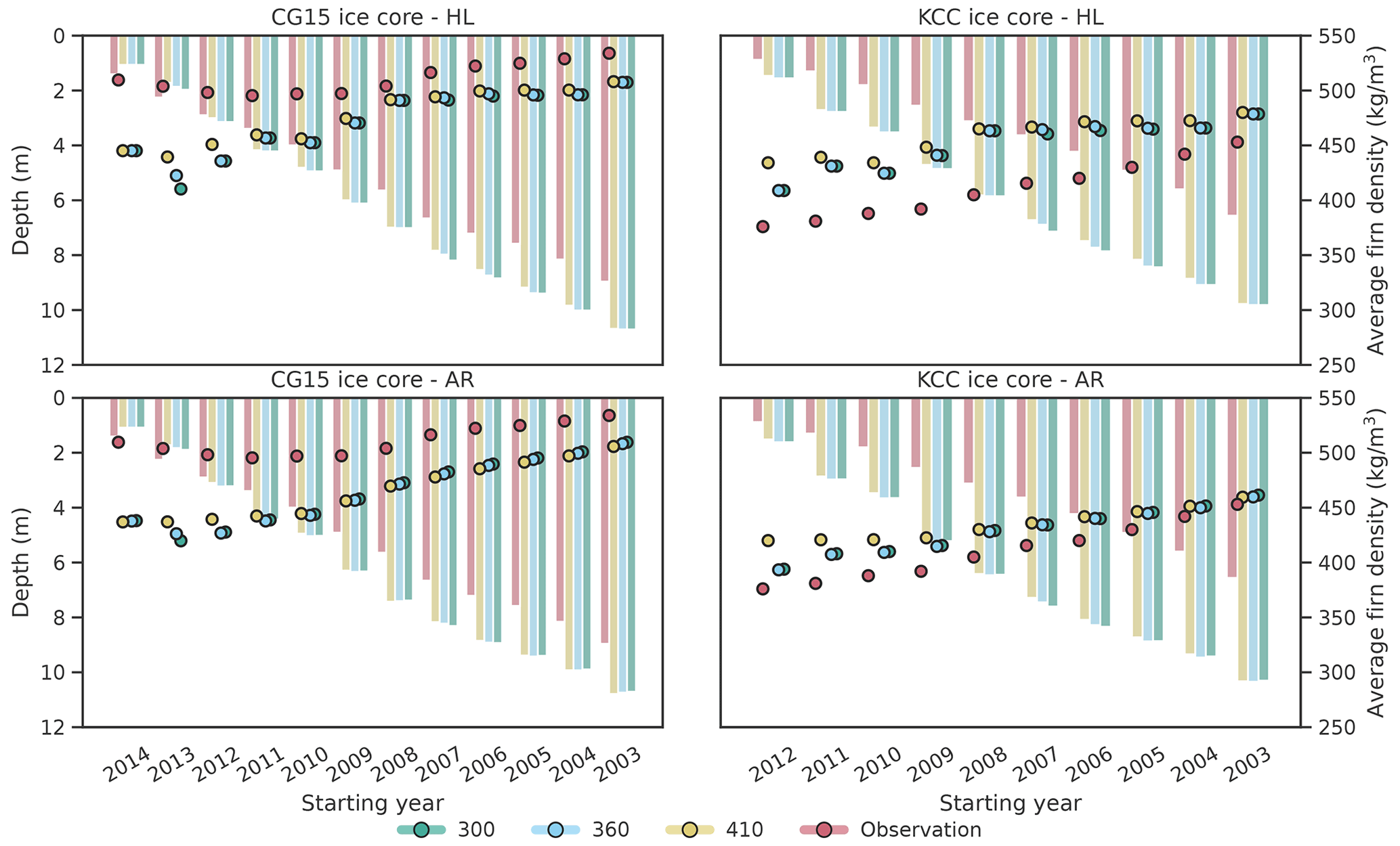
Figure 7Observed and modelled (with one-layer version) average firn density (dots, right axis) and depth (bars, left axis) for KCC and CG15. Each cluster corresponds to a run of the model whose starting date is reported on the x axis. The ending year for all runs is 30 August 2013 for KCC and 30 September 2015 for CG15. AR and HL stand for the model versions with Arnaud et al. (2000) and Herron and Langway (1980) implemented, respectively. The values 300, 360 and 410 stand for the chosen value of ρD.
4.4.2 Multi-layer model version
The modelled density profile was compared with KCC and CG15 density data, implementing in the model both AR and HL (Fig. 8) and testing three different transition densities between snow and firn. Profiles are reported as steps, where each step corresponds to a firn layer. Focusing on the CG15 ice core, we modelled, with both versions, lower densities in the first 4–5 m, with a layer with a particularly low density not matched by the ice core data at around 1–2 m from the surface. This marked decrease however is reduced when a ρD of 410 kg m−3 is chosen. For higher depths, the model with AR implemented underestimates CG15 density, while with HL a better match of the profile is observed. The best performance is obtained implementing HL and selecting , with a mismatch only in the first metres.
Moving to the KCC ice core, the model with AR implemented results in an overestimation of density up to a depth of around 4 m and an underestimation below it. Implementing HL, the density is instead overestimated except for a layer at around 8 m of depth.

Figure 8Observed and modelled (with multi-layer version) firn density profiles for KCC (b, d) and CG15 (a, c). AR and HL stand for the model versions with Arnaud et al. (2000) and Herron and Langway (1980) implemented, respectively.
4.5 Comparison between multi- and single-layer model versions
In order to understand the approximation introduced modelling firn as a single layer instead of a multi-layer column, we compare in Figs. 9–10 the average firn density obtained with the single-layer version of the model or averaging the density of each individual firn layer obtained with the multi-layer version, weighted for their heights. The results for are not reported since they were not significantly different from the ones with . Setting ρD to 360 kg m−3, we have, implementing HL, a maximum difference between the two average densities of 16.7 kg m−3, obtained for the KCC ice core, and, implementing AR, a maximum difference of 7 kg m−3, obtained for the CG15 ice core. Higher differences are obtained moving to , with a maximum difference of 29 and 14 kg m−3 implementing HL and AR, respectively, obtained for the KCC ice core. In all cases the multi-layer version predicts higher average densities.
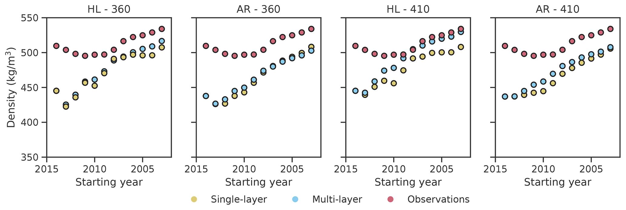
Figure 9Average firn density of CG15 ice core observed and obtained with the single-layer version of the model or averaging the density of each individual firn layer obtained with the multi-layer version, weighted for their heights. Each point corresponds to a run of the model whose starting date is reported on the x axis. The ending year for all runs is 30 September 2015. AR and HL stand for the model versions with Arnaud et al. (2000) and Herron and Langway (1980) implemented, respectively. The values 360 and 410 stand for the chosen value of ρD.

Figure 10Average firn density of KCC ice core observed and obtained with the single-layer version of the model or averaging the density of each individual firn layer obtained with the multi-layer version, weighted for their heights. Each point corresponds to a run of the model whose starting date is reported on the x axis. The ending year for all runs is 30 August 2013. AR and HL stand for the model versions with Arnaud et al. (2000) and Herron and Langway (1980) implemented, respectively. The values 360 and 410 stand for the chosen value of ρD.
5.1 Steady-state firn densification
Figure 4 shows a variable performance of the firn densification model depending on the ice core considered; with the exception of KCC and CG15, which show a very good and a very poor performance, respectively, for all the other cores we have a good fit up to a density of about 600–700 kg m−3. Bréant et al. (2017), who modified the original model of AR, also observed a variable agreement between the data and model, also for sites with similar accumulation and temperature. They suggested that this may be due to different flow regimes of the sites, since their 1D model does not include this effect. Another consideration that emerges from Fig. 4, also pointed out by Bréant et al. (2017), is that the modelled profile results in worse performances when the observed density profile does not show a clear change in the densification rate near the critical density D0. The transition is, in fact, more evident for the KCC ice core, which is associated with the best fit. Finally, Bréant et al. (2017) reported a tendency of the model to overestimate the densification rate for lower densities and to underestimate it for higher densities. This is coherent with the results obtained, in which HL predicts lower densities before D0 and higher densities after D0 if compared with AR. In order to compare modelled and observed profiles in Fig. 4, it is important to point out that the two models assume stationary conditions; therefore they are not able to reproduce possible changes in the glaciological characteristics. In some of the ice cores it is possible to see a bend in the profile in correspondence to about 20–30 m. The reason could be a combination of ice flow and the upstream effect, i.e. changes in snow accumulation upstream, and these effects cannot be reproduced by a 1D model like the ones used.
5.2 Snow accumulation
Snow accumulation at CG is characterized by a high spatial variability (Keck, 2001; Licciulli et al., 2020). The difference in net annual accumulation of CG11 and CG15, which are about 50 m apart, ranges from to in the period 2002–2012, while the one of CG15 and KCC, which are about 120 m apart, ranges between and . Given the high variability in the accumulation rate, three ice cores may not be enough to fully represent the site. In addition, ice core data are biased due to the fact they are drilled preferentially in the north flank, where accumulation is lower. While the modelled average annual accumulation is in the range of the ones estimated for the north flank of CG (Licciulli et al., 2020), the model is not able to reproduce the observed spatial variability. Due to the lack of dependence on topography in the presented model, we do not expect the model to correctly follow one or the other core. The topography influences the amount of solar radiation received, which in turn influences melting and wind erosion. At the same time, the topography modifies wind speed, which in turn modifies topography itself. This results in a quasi-random spatial variation and a systematic temporal variation in surface accumulation at a given location (Keck, 2001). Surface snow temperature was set equal to air temperature, instead of solving the full surface energy balance that would have required a higher availability of data; surface temperatures, in fact, may also reach 0 ∘C for air temperatures below 0 ∘C, mainly when calm conditions are present, or, on the contrary, melting may not occur during positive air temperatures, particularly when wind is present (Keck, 2001).
From the box plots in Fig. 6 we observe that the conserved snow is made up mainly of summer precipitation and that the conserved fraction of solid precipitation reflects the number of hours with greater-than-zero temperature rather than the seasonality of precipitation. The accumulation is, in fact, mainly governed by the wind erosion (Wagenbach et al., 1988) and the presence of wet layers or ice crusts, as well as a faster compaction when temperatures are higher, which protects snow from wind erosion. This is well known in ice core studies at CG, since it results in isotope records that are biased towards precipitation of the warm season (Schöner et al., 2002; Bohleber et al., 2013, 2018). To our knowledge, no models have been applied at CG that try to model the influence of wind speed and temperature on snow accumulation. The only confirmation of this behaviour we have, other than from ice core analysis, comes from temporary measurements of the snow height in nearby sites or observations at CG. For example, at Seserjoch, 4300 , the snow height was measured between 1998 and 2000 by Suter et al. (2001), and a main accumulation from about April to November, with practically no accumulation in high winter, was observed. Assessing the link between temperature, wind speed and snow accumulation may be important under scenarios of climate warming for glacial sites, like CG, whose behaviour is strongly regulated by wind activity. At CG, our results suggest that higher temperatures may lead to a counterintuitive response in the snow mass balance, as already conjectured by Alean et al. (1983). In fact, an increase in melting due to a warmer climate may be compensated for, or exceeded, by the consequent reduction in snow erosion, therefore resulting in a net snow accumulation increase.
5.3 Firn density
5.3.1 One-layer model version
The modelled densities have an opposite behaviour when compared with CG15 or KCC. In the first case, the average density is underestimated and in the second case overestimated. The multi-layer version of the model allows us to better understand the reasons for this mismatch. An error in the density of an individual layer will, in fact, affect all the modelled average firn densities that contain that individual layer. This is the case for CG15, where the underestimation of the density of the most superficial layers (Fig. 8) influences the average density of the whole firn column. This influence however decreases when more annual layers are averaged. In the case of CG15, this is probably related to the characteristics of the CG15 location since underestimation was also observed when applying the firn densification model alone in a steady state and not inside the presented snow–firn model. On the contrary, the steady-state application of HL and AR resulted in a good match with the KCC ice core (Fig. 4). Hence, it is reasonable to suppose that the mismatch is related to the modelled snow characteristics. The discrepancy may be explained by the different estimated surface accumulations; the model, in fact, results in an average snow accumulation of 0.46×10³ against the 0.22×10³ accumulation of KCC. Since the firn densification is driven by overburden stress, this may lead to a systematic bias in the results.
5.3.2 Multi-layer model version
Implementing HL inside the model, we obtained in general a better agreement and a higher variability in the density. The latter is probably related to a higher sensitivity of the equations to surface density, which has instead a low influence on AR as also reported by Bréant et al. (2017). Choosing and looking at the KCC ice core, we observe a decrease in the density at around 7–8 m in both cores. This low density value corresponds to the layer deposited in the 2006–2007 hydrological year. This year was characterized by a solid precipitation event that occurred at the end of the hydrological year. As a consequence, the modelled average snow density decreased from 412 kg m−3 at the beginning of 25 September 2007 to 260.6 kg m−3 at the end of 27 September 2007. Due to the low amount of snow that is not eroded, new solid precipitation events, in fact, may have a high influence on average snow density. The choice of adopting firn densification equations only after a certain density is reached rather than at the end of the water year allows us to better model this circumstance, in which at the end of the water year the layer has characteristics that are more similar to recent snow than to 1-year-old snow. In comparing the observations and model results, it is also important to point out that, due to the differences in firn height between model and ice core, the ages of the modelled and observed steps do not correspond.
The present model does not resolve a full energy balance to compute surface snow temperature, thus not taking into account the effect of the different amount of solar radiation in the different ice core locations, which is very likely responsible for the significantly different behaviours of the two ice cores. The ice core CG15 is closer to the axis saddle and presumably in a location with a higher exposure to solar radiation than KCC since accumulation is doubled. Consequently, melting events may be more frequent in the CG15 ice core. The differences in the model parameters when run for the KCC or CG15 ice core are the values of MAFT, ρD and γ′ when AR is implemented, and this limits the ability of the model to adapt to the different ice cores.
In this study we have proposed a local model that combines snow and firn dynamics. It was derived from the mass balance, momentum balance and rheological equations of snow and firn, combined with semi-empirical and empirical approaches proposed in the literature to model the included mass fluxes. It requires for input hourly (or sub-hourly) series of precipitation, temperature and wind speed with which the series of snow, water and ice inside the snowpack and firn height along with dry-snow and firn density are computed. Two versions of the model were proposed: (1) a version (multi-layer) that considers separately each firn layer and (2) a version (single-layer) that models firn and underlying glacier ice as a single layer. The two implementations allow us to cover different purposes. A simpler model is, in fact, more suitable to reproducing firn inside a hydrological model, where the whole depth–density profile is not necessary and where a reduced number of equations may allow an easier integration. On the other hand, a model that resolves density with depth allows us to assess the influence of meteorological variables on snow and firn characteristics. In order to obtain this, we integrated two existing firn densification models (other firn densification models could possibly be implemented) into a wider model, therefore moving the boundary of the model from surface accumulation and density to hourly meteorological series. While this may not be needed to retrieve past climatological information from ice cores, it is required to assess the response of the system to present and future changes in the climate.
Both models' versions require the calibration of three parameters: a, e and γ′. In addition, the parameters of the firn densification equation chosen may also need calibration if applied to a temperate site. The modularity of the model allows us to easily test different modelizations of the included fluxes. Depending also on the availability of measured data at the application site, less empirical approaches could be adopted for the mass fluxes. Also, depending on the specific application, some processes presented in the model may be neglected with a reduction in the total number of parameters. A high number of parameters are, for example, associated with wind effects that may be neglected in lower-altitude sites but that are likely to be important in high-altitude sites (Haeberli and Alean, 1985). At Colle Gnifetti, for example, we saw that observed surface accumulations and densities cannot be explained if wind effects are not considered. The modelled reduction in annual snow accumulation due to wind erosion is on average 2×10³ while the increase in end-of-year snow density is on average 65 kg m−3. The strong wind erosion also results in a greater correlation between the amount of snow preserved in each month and the number of days with above-zero temperature rather than with the solid precipitation seasonality. This behaviour may be important in understanding the response of the site to a warming climate. All these elements result in a strong spatial and temporal variability in snow density and accumulation at CG that is not captured by the model. This would, in fact, require taking into consideration the influence of topography on wind speed and the effect of solar radiation on surface snow temperature.
The aim of this study was to illustrate the new snow–firn modelling and to present its potentiality through a case study. In order to integrate it into a hydrological model, further steps are required; in particular fluxes among the different columns should be properly considered regarding both run-off and snow transport. In the present modelling, for example, we considered only the snow erosion. At CG the deposition can be neglected due to its characteristics. The site is a saddle with west–east orientation where the predominant wind direction coincides with the saddle orientation. Besides, an ice cliff at the end of it works as a perfect sink for the eroded snow. A distributed modelling approach needs to take into account the presence of sinks and sources of snow transport. This will also improve the representation of wind effects on snow accumulation since, in order to include snow transport in a 1D framework, approximation of the process is unavoidable for the nature of the process itself.
A1 Mass balance equations
The mass balance equations of snow (MS), liquid water in snow (MW), refrozen meltwater and rain in snow (MMF), and firn (MF) are as follows:
PS and PR are the mass of solid and liquid precipitation events, and they are equal to and . The fresh-snow density was calculated as proposed by Liston et al. (2007): . Following Anderson (1976), kg m−3 if the air temperature and kg m−3 otherwise. The second term gives the increase in fresh-snow density due to wind, and it is computed as , where u2 is the wind speed at a 2 m height, D1=25 kg m−3, D2=250.0 kg m−3 and D3=0.2 s m−1. When u2≤5 m s−1, kg m−3.
M is the snowmelt mass flux that was computed with a temperature-index approach (Hock, 2003): .
F is the melt–freeze mass flux that was modelled with a coupled melt–freeze temperature-index approach: .
The run-off O was modelled with a matrix flow approach, and it is equal to O=ρWαKW, where ) (DeWalle and Rango, 2008) with . Following Colbeck (1972), KW was computed as , in which K is the intrinsic permeability of snow in square metres and S* is the effective saturation degree of the mixture equal to with being the irreducible saturation degree equal to (Kelleners et al., 2009) and Sr the average saturation degree of the porous matrix equal to 1 when hW≥ϕhS and equal to otherwise (Avanzi et al., 2015). The intrinsic permeability is obtained using the parametrization proposed by Calonne et al. (2012), and it is equal to , in which R is the equivalent sphere radius. The radius R is defined as , where SSA is the specific surface area in m2 kg−1 that was computed by Avanzi et al. (2015) adapting the formula proposed by Domine et al. (2007) with . When Sr>0.5, to avoid numerical instability, the run-off is calculated with a kinematic wave approximation (De Michele et al., 2013) as .
The firn melting OF, which may occur only when the snowpack is absent, was modelled with a temperature-index approach, and it is equal to .
PF is the effect of rain on firn that, when the snowpack is absent, causes an increase in MF when TA<0 ∘C because rainfall is chilled to the firn temperature and a decrease when TA>0 ∘C because the energy supplied by rain will be used to melt ice. In the first case , while in the second case PF was set to zero due to its small contribution to mass balance (Doyle et al., 2015).
The terms ES, EW and EMF move the mass of the snowpack still on the ground at the end of each melt season inside the firn, and they are equal to with j denoting S, MF and W.
Q is the mass of snow eroded by wind obtained from snow transport. The latter was computed adopting the parametrization proposed by Pomeroy et al. (1993) as the sum of a transport in saltation and a transport in suspension.
The saltation transport rate Qsalt () occurs only when wind exceeds a given threshold, and it is computed as follows:
where ρa is the atmospheric density (kg m−3) and u* and are the atmospheric friction velocity and the friction velocity applied to the snow surface at the transport threshold, respectively (m s−1). To move from the measured wind speed u to u*, knowledge of the aerodynamic roughness height z0 is required. This passage is not straightforward since the value of z0 during blowing snow events is different from the one during non-transport conditions and it depends on friction velocity (Pomeroy and Gray, 1990). In order to avoid an iterative procedure, we adopted the approximation proposed by Pomeroy and Gray (1990), using and , where u is the 10 m wind speed (m s−1).
Suspension transport, which occurs only when particles are already in saltation, was computed as follows:
where Qsusp is in , κ is the von Kármán constant equal to 0.4, h* is the lower boundary for suspension equal to (Pomeroy and Male, 1992) with , zb is the top of the surface boundary layer for suspended snow and η(z) is the mass concentration of suspended snow (kg m−3) at height z. The mass concentration can be approximate as (Pomeroy and Male, 1992), where η(zr) is the reference mass concentration for suspension set to 0.8 kg m−3 (Pomeroy and Male, 1992), AQ is equal to 1.55 m0.544 and BQ is equal to 0.05628 s−0.544. zb was set to 5 m since its value is typically between 5 and 10 m (Déry and Taylor, 1996). The exact value is unimportant because of small mass fluxes at this height (Pomeroy et al., 1993). The snow erosion in the control volume of the model was set equal to the sum of these two transports.
The critical threshold above which snow transport occurs was computed adopting the formula proposed by He and Ohara (2017). The critical shear stress for snow movement can be therefore computed as follows:
where R is the grain radius (m); td is the time since deposition in seconds; Cc, Cd, Cg and Cl are dimensionless coefficients set to 1, 4, and 3.4 (He and Ohara, 2017); ς is the stress caused by cohesion of ice computed as (Hosler et al., 1957) for temperatures between −20 and 0 ∘C with ς in newtons per square metre and TA in degrees Celsius; and . C, m and n are parameters that influence the rate of ice sintering, modelled following Maeno and Arakawa (2004). In particular, , in which RG is the gas constant and TA is computed as the average air temperature since deposition, m3 s−1, and J mol−1. Finally, m and n are empirical parameters set to 2.9 and 5, respectively, following the results of He and Ohara (2017). Once the critical shear stress is obtained, it is possible to move to the critical friction velocity as follows: . If wind speed is lower than the critical threshold, no erosion occurs and Q is set to zero.
To implement the snow erosion routine, we proceeded as explained in the following. When the first solid precipitation event occurs in a time step, the amount of new snow on the ground at the end of the time step, SA (), is saved along with the time of deposition and ρNS of the event. During the following step, four different situations are possible: (1) a new snow event occurs in the time step. In this case SA is moved into a vector SR with its time of deposition and ρNS. SA is recomputed as ρNS⋅s. (2) TA>0 ∘C. In this case SA and Q are set to 0 , and all the old snow events memorized in SR are removed. (3) TA<0 ∘C and Q<SA. In this case SA is set to . (4) TA<0 ∘C and Q>SA. In this case, if SR has no elements, Q is set equal to SA and SA to 0 ; otherwise the difference between Q and SA is subtracted from the most recent event in SR, given that wind speed is higher than the threshold recomputed with the characteristics of that event, and this event is removed from SR. This is repeated until an event in SR that cannot be eroded by wind is encountered or the total amount of snow eroded in that time step reaches Q. In the latter case the actual transport is Q, while in the former Q is given by the total amount of snow eroded before reaching the non-erodible layer. The new SA is the amount of snow associated with the last event considered.
Given that Mj=ρjhj and ρk=const with j denoting S, MF, and W and k denoting MF and W, after some algebra we can move from Eqs. (A1a)–(A1d) to Eqs. (2a)–(2d).
A2 Snow densification
The densification of dry snow due to compaction was modelled adopting the formula proposed by Liston et al. (2007):
where , A1=0.0013 m−1, , and U is the wind speed contribution (m s−1). For wind speeds , , with E1, E2 and E3 equal to 5.0 m s−1, 15.0 and 0.2 s m−1, respectively, and u2 is the wind speed at a 2 m height. For wind speed , . Adding the densification due to mass variation (see De Michele et al., 2013), the total densification rate can be computed as follows:
where we assumed that melting events and snow erosion occur at ρS=const.
A3 Arnaud et al. (2000) model
The model of AR separates the densification of firn into three stages. The first stage is governed by settling, and it is modelled by Bréant et al. (2017) adapting the equation proposed by Alley (1987). The second stage, which starts when the relative density equals D0, is dominated by power law creep, and it is modelled following Arzt (1982) and Arzt et al. (1983). Grains are considered spheres, and each sphere is allowed to increase in radius around fixed centres. Starting from an initial radius l, the new radius l′ (in units of the initial particle radius l) is . The growth of spheres increases the number of particle contacts Z from the initial value Z0 to , in which b=15.5. The overlap due to the growth of particles produces an excess volume of material. This excess is distributed uniformly around the portion of the surface of the spheres not in contact. From this excess volume, it is possible to calculate the new radius l′′ as
The average contact area (in units of l2) can be obtained averaging over all existing contacts:
The value of Z0 for a given value of D0 is obtained, as proposed by Arnaud et al. (2000), assuming that the effective stress approaches P as D tends to 1. The third stage begins when pores start becoming isolated (D>Dc) and densification is calculated considering the deformation of ice shells surrounding cylindrical pores (Wilkinson and Ashby, 1975). As for Eq. (2e), the total densification rate is obtained adding the densification due to new mass addition (Eq. 2f).
Table B1List of the symbols and abbreviations used in the mass fluxes of the snow–firn model with the exclusion of snow erosion (from A to S).
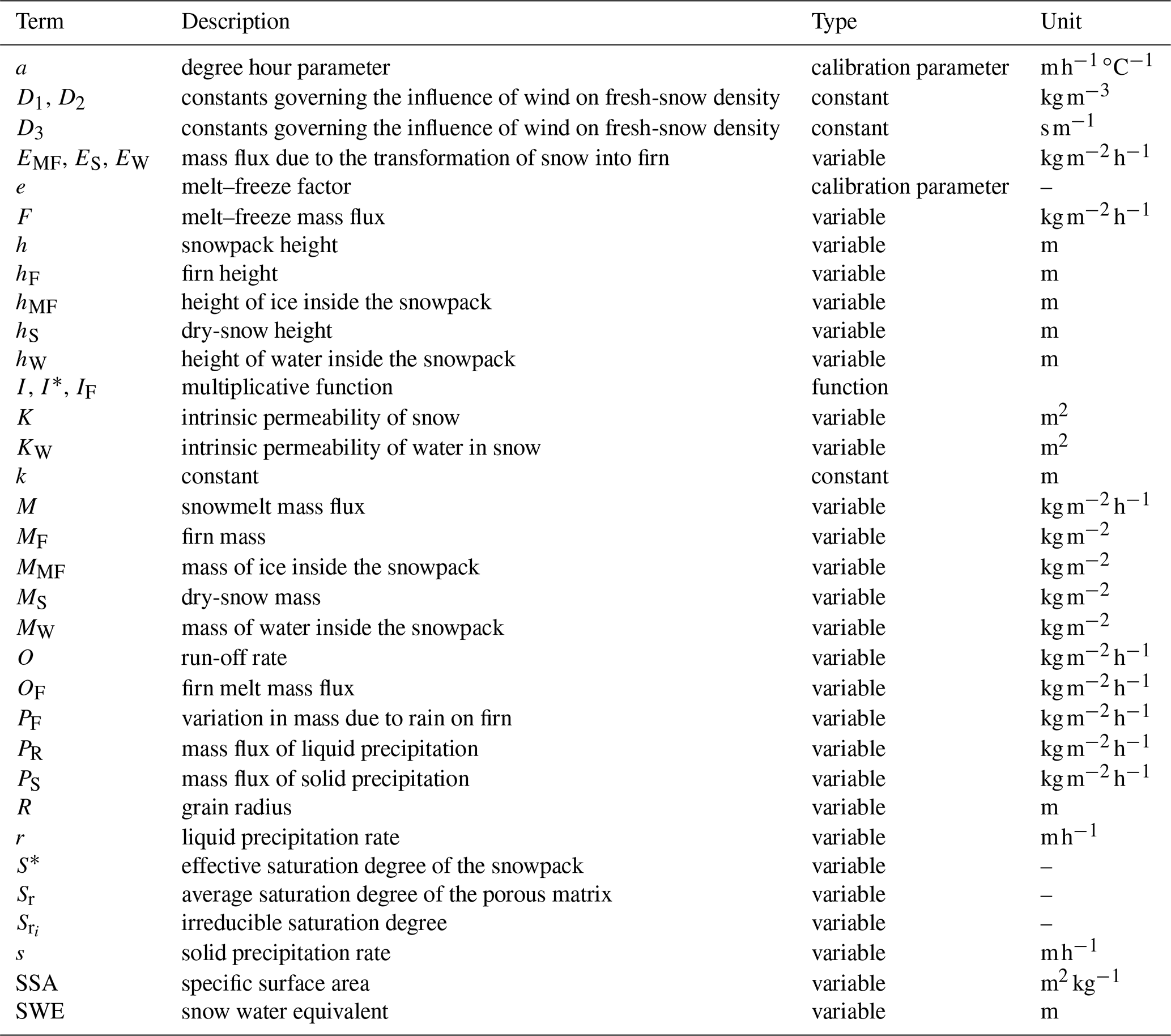
Table B2List of the symbols used in the mass fluxes of the snow–firn model with the exclusion of snow erosion (from T to Z and Greek letters).
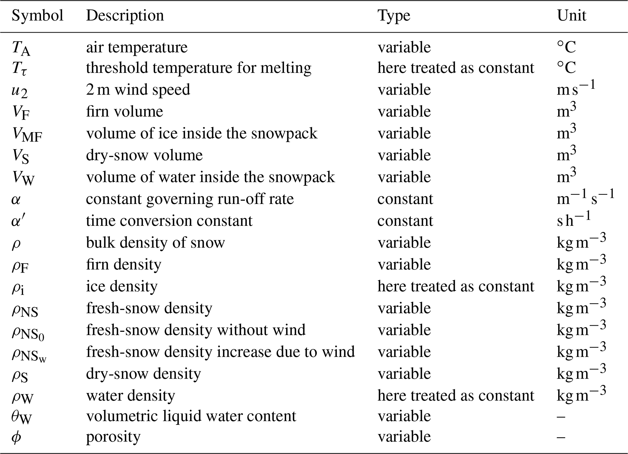
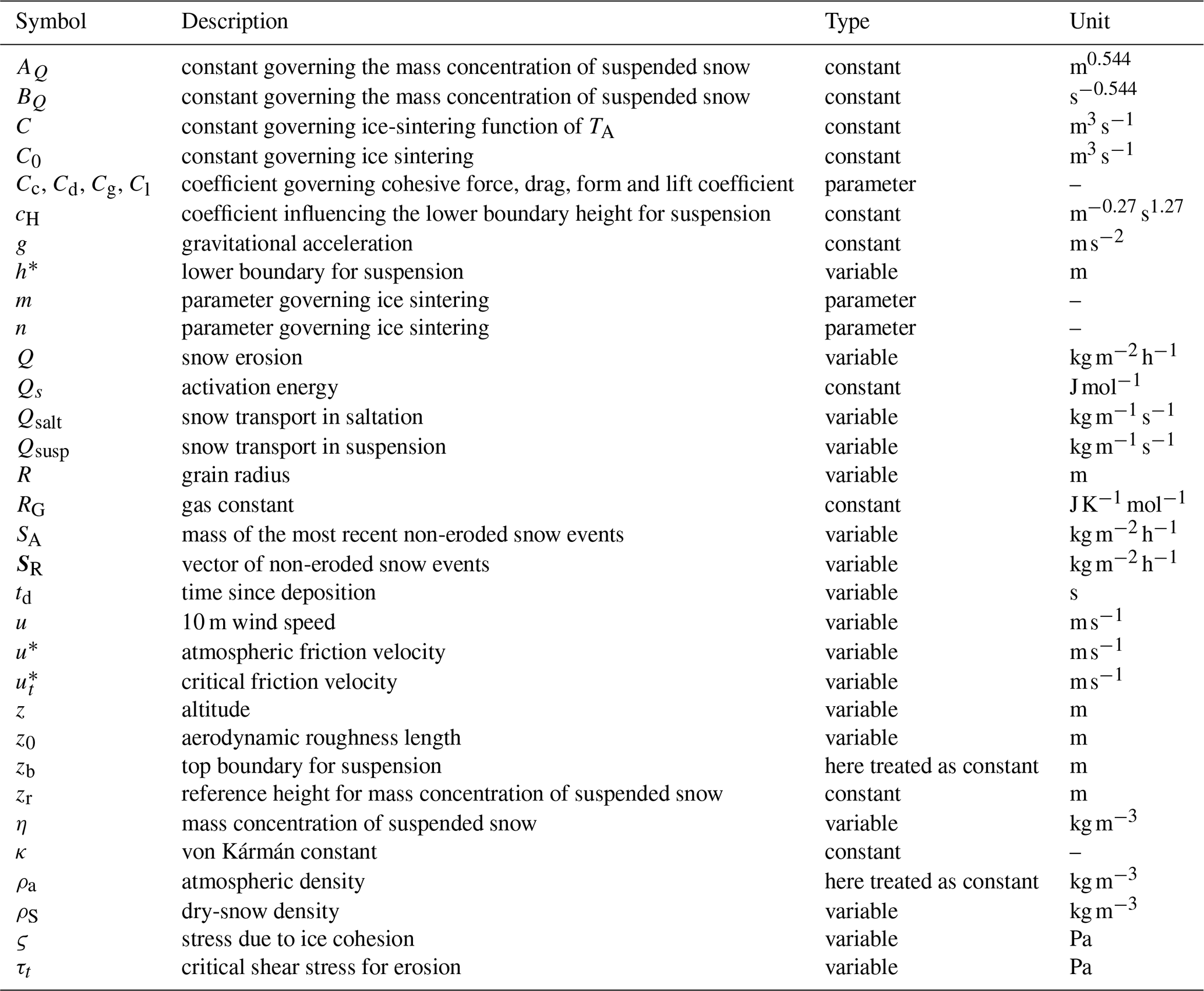

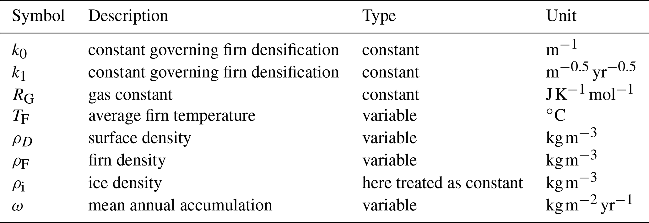
Table B6List of the symbols related to snow densification rate.

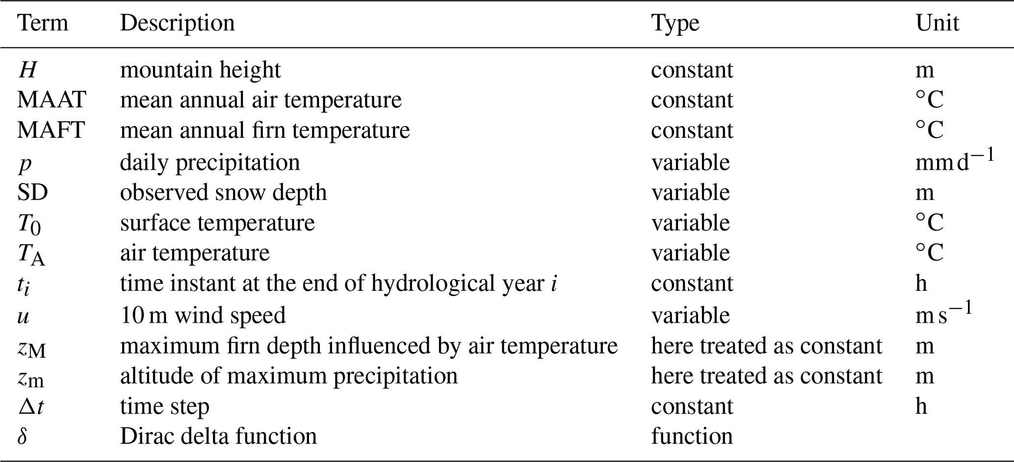
Table B7List of other symbols and abbreviations used throughout the paper.
Meteorological data measured by the network of stations of the Aosta Valley Region can be downloaded from https://presidi2.regione.vda.it/str_dataview (last access: 11 March 2022). Snow water equivalent and snow density data must be requested directly from the Aosta Valley Region. Hourly meteorological data of the network of stations in Piemonte must be requested from the region, and they are free of charge for research purposes. Wind data at Col du Grand St Bernard come from from the Integrated Surface Dataset (ISD), maintained by the National Oceanic and Atmospheric Administration (NOAA), and they can be accessed from https://www.ncei.noaa.gov/metadata/geoportal/rest/metadata/item/gov.noaa.ncdc:C00532/html (NOAA National Centers for Environmental Information, 2001). B76 and B77 ice core data are published in the following paper: https://doi.org/10.3189/S0022143000005220 (Gäggeler et al., 1983). CG03 and CG15 are available on the PANGAEA repository (https://doi.org/10.1594/PANGAEA.894787, Sigl et al., 2018). CG11 ice core data are published in the following thesis: http://hdl.handle.net/10579/1924 (Ardenghi, 2012). The other ice core data were requested from the authors.
CDM and FB conceived the model. FB took care of data and developed the case study. FB wrote a first draft of the manuscript. FB and CDM reviewed the manuscript.
The contact author has declared that neither they nor their co-author has any competing interests.
Publisher’s note: Copernicus Publications remains neutral with regard to jurisdictional claims in published maps and institutional affiliations.
We would like to thank ARPA Piemonte for the meteorological data used in this study, with particular thanks to Manuela Bassi, and Aosta Valley for the snow water equivalent data. Gratitude is also due to Carlo Licciulli and Josef Lier for ice core data and to Pascal Bohleber for the information about Colle Gnifetti. Thank you to Scenari Digitali and Rifugi Monterosa for additional information about Capanna Regina Margherita. We would also like to thank the editors, Olaf Eisen and Michiel van den Broeke, and the three anonymous referees for their comments and feedback about the manuscript (including about a previous submission of the manuscript).
This paper was edited by Michiel van den Broeke and reviewed by two anonymous referees.
Adhikary, S. P.: Inaugural address, in: Snow and glacier hydrology, edited by: Young, G. J., International Association of Hydrological Sciences (IAHS), Wallingford, Oxfordshire OX10 8BB, UK, ISBN 0-947571-83-3, 1993. a
Aizen, V. B., Aizen, E. M., and Melack, J. M.: Precipitation, melt and runoff in the northern Tien Shan, J. Hydrol., 186, 229–251, https://doi.org/10.1016/S0022-1694(96)03022-3, 1996. a
Alean, J., Haeberli, W., and Schädler, B.: Snow accumulation, firn temperature and solar radiation in the area of the Colle Gnifetti core drilling site (Monte Rosa, Swiss Alps): distribution patterns and interrelationships, Zeitschrift für Gletscherkunde und Glazialgeologie, 19, 131–147, 1983. a, b, c, d
Alley, R. B.: Firn densification by grain-boundary sliding: a first model, J. Phys. Colloques, 48, C1-249–C1-256, https://doi.org/10.1051/jphyscol:1987135, 1987. a
Alpert, P.: Mesoscale Indexing of the Distribution of Orographic Precipitation over High Mountains, J. Clim. Appl. Meteor., 25, 532–545, https://doi.org/10.1175/1520-0450(1986)025<0532:MIOTDO>2.0.CO;2, 1986. a
Anderson, E. A.: A point energy and mass balance model of a snow cover, vol. 19, NOAA Technical Report NWS, 19, United States, National Weather Service, https://repository.library.noaa.gov/view/noaa/6392 (last access: 2 March 2022), 1976. a
Ardenghi, N.: Geochemical characterization of a shallow firn core retrieved from Colle Gnifetti (Monte Rosa, Italy), Master's thesis, Università Ca'Foscari Venezia, Italy, http://hdl.handle.net/10579/1924 (last access: 2 March 2022), 2012. a, b
Arnaud, L., Barnola, J. M., and Duval, P.: Physical modeling of the densification of snow/firn and ice in the upper part of polar ice sheets, in: Physics of ice core records, edited by: Hondoh, T., Hokkaido University Press, Sapporo, Japan, pp. 285–305, http://hdl.handle.net/2115/32472 (last access: 2 March 2022), 2000. a, b, c, d, e, f, g, h, i, j, k
Arthern, R. J., Vaughan, D. G., Rankin, A. M., Mulvaney, R., and Thomas, E. R.: In situ measurements of Antarctic snow compaction compared with predictions of models, J. Geophys. Res.-Earth, 115, F03011, https://doi.org/10.1029/2009JF001306, 2010. a
Arzt, E.: The influence of an increasing particle coordination on the densification of spherical powders, Acta Metall. Mater., 30, 1883–1890, https://doi.org/10.1016/0001-6160(82)90028-1, 1982. a
Arzt, E., Ashby, M. F., and Easterling, K. E.: Practical applications of hotisostatic pressing diagrams: four case studies, Metall. Mater. Trans. A, 14, 211–221, https://doi.org/10.1007/BF02651618, 1983. a
Avanzi, F., De Michele, C., Ghezzi, A., Jommi, C., and Pepe, M.: A processing- modeling routine to use SNOTEL hourly data in snowpack dynamic models, Adv. Water Resour., 73, 16–29, https://doi.org/10.1016/j.advwatres.2014.06.011, 2014. a, b, c, d
Avanzi, F., Yamaguchi, S., Hirashima, H., and De Michele, C.: Bulk volumetric liquid water content in a seasonal snowpack: modeling its dynamics in different climatic conditions, Adv. Water Resour., 86, 1–13, https://doi.org/10.1016/j.advwatres.2015.09.021, 2015. a, b, c, d, e, f, g, h, i, j
Bader, H.: Sorge's Law of densification of snow on high polar glaciers, J. Glaciol., 2, 319–323, https://doi.org/10.3189/S0022143000025144, 1954. a
Bainov, D. and Simeonov, P.: Impulsive differential equations: periodic solutions and applications, 1st edn., vol. 66, Longman, England, ISBN 978-0582096394, 1993. a
Benn, D. I. and Evans, D. J. A.: Glaciers and glaciation, second edn., Hodder Education, London, ISBN 9780340905791, 2010. a
Bohleber, P., Wagenbach, D., Schöner, W., and Böhm, R.: To what extent do water isotope records from low accumulation Alpine ice cores reproduce instrumental temperature series?, Tellus B, 65, 20148, https://doi.org/10.3402/tellusb.v65i0.20148, 2013. a
Bohleber, P., Erhardt, T., Spaulding, N., Hoffmann, H., Fischer, H., and Mayewski, P.: Temperature and mineral dust variability recorded in two low-accumulation Alpine ice cores over the last millennium, Clim. Past, 14, 21–37, https://doi.org/10.5194/cp-14-21-2018, 2018. a, b
Bréant, C., Martinerie, P., Orsi, A., Arnaud, L., and Landais, A.: Modelling firn thickness evolution during the last deglaciation: constraints on sensitivity to temperature and impurities, Clim. Past, 13, 833–853, https://doi.org/10.5194/cp-13-833-2017, 2017. a, b, c, d, e, f, g, h
Calonne, N., Geindreau, C., Flin, F., Morin, S., Lesaffre, B., Rolland du Roscoat, S., and Charrier, P.: 3-D image-based numerical computations of snow permeability: links to specific surface area, density, and microstructural anisotropy, The Cryosphere, 6, 939–951, https://doi.org/10.5194/tc-6-939-2012, 2012. a
Colbeck, S.: A theory of water percolation in snow, J. Glaciol., 11, 369–385, https://doi.org/10.3189/S0022143000022346, 1972. a
Cuffey, K. M. and Paterson, W. S. B.: The physics of glaciers, fourth edn., Butterworth Heinemann-Elsevier, Burlington, ISBN 9780123694614, 2010. a, b, c, d
De Michele, C., Avanzi, F., Ghezzi, A., and Jommi, C.: Investigating the dynamics of bulk snow density in dry and wet conditions using a one-dimensional model, The Cryosphere, 7, 433–444, https://doi.org/10.5194/tc-7-433-2013, 2013. a, b, c, d, e, f, g, h
Déry, S. J. and Taylor, P. A.: Some aspects of the interaction of blowing snow with the atmospheric boundary layer, Hydrol. Process., 10, 1345–1358, https://doi.org/10.1002/(SICI)1099-1085(199610)10:10<1345::AID-HYP465>3.0.CO;2-2, 1996. a, b
DeWalle, D. R. and Rango, A.: Principles of snow hydrology, Cambridge University Press, New York, https://doi.org/10.1017/CBO9780511535673, 2008. a, b
Domine, F., Taillandier, A.-S., and Simpson, W. R.: A parameterization of the specific surface area of seasonal snow for field use and for models of snowpack evolution, J. Geophys. Res.-Earth, 112, F02031, https://doi.org/10.1029/2006JF000512, 2007. a, b
Doyle, S. H., Hubbard, A., Van De Wal, R. S., Box, J. E., Van As, D., Scharrer, K., Meierbachtol, T. W., Smeets, P. C., Harper, J. T., and Johansson, E.: Amplified melt and flow of the Greenland ice sheet driven by late-summer cyclonic rainfall, Nat. Geosci., 8, 647–653, https://doi.org/10.1038/ngeo2482, 2015. a
Duan, Q., Sorooshian, S., and Gupta, V.: Effective and efficient global optimization for conceptual rainfall-runoff models, Water Resour. Res., 28, 1015–1031, https://doi.org/10.1029/91WR02985, 1992. a
Duan, Q. Y., Gupta, V. K., and Sorooshian, S.: Shuffled complex evolution approach for effective and efficient global minimization, J. Optimiz. Theory App., 76, 501–521, https://doi.org/10.1007/BF00939380, 1993. a
Eichler, A., Schwikowski, M., Gäggeler, H. W., Furrer, V., Synal, H.-A., Beer, J., Saurer, M., and Funk, M.: Glaciochemical dating of an ice core from upper Grenzgletscher (4200 m a.s.l.), J. Glaciol., 46, 507–515, https://doi.org/10.3189/172756500781833098, 2000. a
Fountain, A. G. and Tangborn, W. V.: The Effect of Glaciers on Streamflow Variations, Water Resour. Res., 21, 579–586, https://doi.org/10.1029/WR021i004p00579, 1985. a
Gäggeler, H., von Gunten, H. R., Rössler, E., Oeschger, H., and Schotterer, U.: 210Pb dating of Cold Alpine Firn/Ice Cores From Colle Gnifetti, Switzerland, J. Glaciol., 29, 165–177, https://doi.org/10.3189/S0022143000005220, 1983. a, b, c
Haeberli, W. and Alean, J.: Temperature and accumulation of high altitude firn in the Alps, Ann. Glaciol., 6, 161–163, https://doi.org/10.3189/1985AoG6-1-161-163, 1985. a, b
Haeberli, W. and Funk, M.: Borehole temperatures at the Colle Gnifetti core-drilling site (Monte Rosa, Swiss Alps), J. Glaciol., 37, 37–46, https://doi.org/10.3189/S0022143000042775, 1991. a
Hagg, W., Braun, L. N., Kuhn, M., and Nesgaard, T. I.: Modelling of hydrological response to climate change in glacierized Central Asian catchments, J. Hydrol., 332, 40–53, https://doi.org/10.1016/j.jhydrol.2006.06.021, 2007. a
He, S. and Ohara, N.: A New Formula for Estimating the Threshold Wind Speed for Snow Movement, J. Adv. Model. Earth Sy., 9, 2514–2525, https://doi.org/10.1002/2017MS000982, 2017. a, b, c
Henn, B., Raleigh, M. S., Fisher, A., and Lundquist, J. D.: A comparison of methods for filling gaps in hourly near-surface air temperature data, J. Hydrometeorol., 14, 929–945, https://doi.org/10.1175/JHM-D-12-027.1, 2013. a
Herron, M. M. and Langway, C. C.: Firn Densification: An Empirical Model, J. Glaciol., 25, 373–385, https://doi.org/10.1017/S0022143000015239, 1980. a, b, c, d, e, f, g
Hock, R.: Temperature index melt modelling in mountain areas, J. Hydrol., 282, 104–115, https://doi.org/10.1016/S0022-1694(03)00257-9, 2003. a
Hock, R., Jansson, P., and Braun, L. N.: Modelling the Response of Mountain Glacier Discharge to Climate Warming, in: Global Change and Mountain Regions: An Overview of Current Knowledge, edited by: Huber, U. M., Bugmann, H. K. M., and Reasoner, M. A., Adv. Glob. Change Res., 23, 243–252, Springer, Dordrecht, the Netherlands, ISBN 978-1-4020-3508-1, https://doi.org/10.1007/1-4020-3508-X_25, 2005. a
Hock, R., Rasul, G., Adler, C., Cáceres, B., Gruber, S., Hirabayashi, Y., Jackson, M., Kääb, A., Kang, S., Kutuzov, S., Milner, A., Molau, U., Morin, S., Orlove, B., and Steltzer, H.: High Mountain Areas, in: IPCC Special Report on the Ocean and Cryosphere in a Changing Climate, edited by: Pörtner, H.-O., Roberts, D. C., Masson-Delmotte, V., Zhai, P., Tignor, M., Poloczanska, E., Mintenbeck, K., Alegría, A., Nicolai, M., Okem, A., Petzold, J., Rama, B., and Weyer, N. M., in press, https://www.ipcc.ch/srocc/chapter/chapter-2/ (last access: 2 March 2022), 2019. a
Hosler, C. L., Jensen, D. C., and Goldshlak, L.: On the aggregation of ice crystals to form snow, J. Meteor., 14, 415–420, https://doi.org/10.1175/1520-0469(1957)014<0415:OTAOIC>2.0.CO;2, 1957. a
Huss, M.: Density assumptions for converting geodetic glacier volume change to mass change, The Cryosphere, 7, 877–887, https://doi.org/10.5194/tc-7-877-2013, 2013. a, b
Huss, M., Jouvet, G., Farinotti, D., and Bauder, A.: Future high-mountain hydrology: a new parameterization of glacier retreat, Hydrol. Earth Syst. Sci., 14, 815–829, https://doi.org/10.5194/hess-14-815-2010, 2010. a, b, c
Hyndman, R. J. and Athanasopoulos, G.: Forecasting: principles and practice, 3rd edn., OTexts: Melbourne, Australia, http://Otexts.com/fpp3 (last access: 2 March 2022), 2021. a
Jacka, T. and Jun, L.: The steady-state crystal size of deforming ice, Ann. Glaciol., 20, 13–18, https://doi.org/10.3189/1994AoG20-1-13-18, 1994. a
Jansson, P., Hock, R., and Schneider, T.: The concept of glacier storage: a review, J. Hydrol., 282, 116–129, https://doi.org/10.1016/S0022-1694(03)00258-0, 2003. a
Jennings, K. S., Winchell, T. S., Livneh, B., and Molotch, N. P.: Spatial variation of the rain-snow temperature threshold across the Northern Hemisphere, Nat. Commun., 9, 1148, https://doi.org/10.1038/s41467-018-03629-7, 2018. a
Jost, G., Moore, R. D., Menounos, B., and Wheate, R.: Quantifying the contribution of glacier runoff to streamflow in the upper Columbia River Basin, Canada, Hydrol. Earth Syst. Sci., 16, 849–860, https://doi.org/10.5194/hess-16-849-2012, 2012. a, b
Keck, L.: Climate significance of stable isotope records from Alpine ice cores, PhD thesis, Institute of Environmental Physics, Heidelberg University, Germany, https://doi.org/10.11588/heidok.00001837, 2001. a, b, c
Kelleners, T., Chandler, D., McNamara, J. P., Gribb, M. M., and Seyfried, M.: Modeling the water and energy balance of vegetated areas with snow accumulation, Vadose Zone J., 8, 1013–1030, https://doi.org/10.2136/vzj2008.0183, 2009. a
Lehning, M., Doorschot, J., and Bartelt, P.: A snowdrift index based on SNOWPACK model calculations, Ann. Glaciol., 31, 382–386, https://doi.org/10.3189/172756400781819770, 2000. a
Li, L. and Pomeroy, J. W.: Estimates of Threshold Wind Speeds for Snow Transport Using Meteorological Data, J. Appl. Meteorol., 36, 205–213, https://doi.org/10.1175/1520-0450(1997)036<0205:EOTWSF>2.0.CO;2, 1997. a
Licciulli, C., Bohleber, P., Lier, J., Gagliardini, O., Hoelzle, M., and Eisen, O.: A full Stokes ice-flow model to assist the interpretation of millennial-scale ice cores at the high-Alpine drilling site Colle Gnifetti, Swiss/Italian Alps, J. Glaciol., 66, 35–48, https://doi.org/10.1017/jog.2019.82, 2020. a, b, c, d, e, f, g
Liston, G. E. and Elder, K.: A meteorological distribution system for high-resolution terrestrial modeling (MicroMet), J. Hydrometeorol., 7, 217–234, https://doi.org/10.1175/JHM486.1, 2006. a
Liston, G. E., Haehnel, R. B., Sturm, M., Hiemstra, C. A., Berezovskaya, S., and Tabler, R. D.: Simulating complex snow distributions in windy environments using SnowTran-3D, J. Glaciol., 53, 241–256, https://doi.org/10.3189/172756507782202865, 2007. a, b, c
Lundin, J. M., Stevens, C. M., Arthern, R., Buizert, C., Orsi, A., Ligtenberg, S. R., Simonsen, S. B., Cummings, E., Essery, R., Leahy, W., Harris, P., Helsen M. M., and Waddington E. D.: Firn Model Intercomparison Experiment (FirnMICE), J. Glaciol., 63, 401–422, https://doi.org/10.1017/jog.2016.114, 2017. a
Luo, Y., Arnold, J., Liu, S., Wang, X., and Chen, X.: Inclusion of glacier processes for distributed hydrological modeling at basin scale with application to a watershed in Tianshan Mountains, northwest China, J. Hydrol., 477, 72–85, https://doi.org/10.1016/j.jhydrol.2012.11.005, 2013. a
Lüthi, M. and Funk, M.: Dating ice cores from a high Alpine glacier with a flow model for cold firn, Ann. Glaciol., 31, 69–79, https://doi.org/10.3189/172756400781820381, 2000. a, b, c, d, e, f
Maeno, N. and Arakawa, M.: Adhesion shear theory of ice friction at low sliding velocities, combined with ice sintering, J. Appl. Phys., 95, 134–139, https://doi.org/10.1063/1.1633654, 2004. a
Mariani, I., Eichler, A., Jenk, T. M., Brönnimann, S., Auchmann, R., Leuenberger, M. C., and Schwikowski, M.: Temperature and precipitation signal in two Alpine ice cores over the period 1961–2001, Clim. Past, 10, 1093–1108, https://doi.org/10.5194/cp-10-1093-2014, 2014. a, b
Martorina, S., Olivero, A., Loglisci, N., Pelosini, R., and Paesano, G.: Capanna Margherita – The highest meteorological station in Europe. Is it possible to consider it as representative of synoptic weather?, in: International Conference on Alpine Meteorology and MAP-Meeting, Brig, Switzerland, 19–23 May 2003, https://www.researchgate.net/publication/261237335_Capanna_Margherita_-_The_highest_meteorological_station_in_Europe_Is_it_possible_to_consider_it_as_representative_of_synoptic_weather (last access: 2 March 2022), 2003. a
Naz, B. S., Frans, C. D., Clarke, G. K. C., Burns, P., and Lettenmaier, D. P.: Modeling the effect of glacier recession on streamflow response using a coupled glacio-hydrological model, Hydrol. Earth Syst. Sci., 18, 787–802, https://doi.org/10.5194/hess-18-787-2014, 2014. a, b
NOAA National Centers for Environmental Information: Global Surface Hourly [station used: ID 06717099999], NOAA National Centers for Environmental Information [data set], https://www.ncei.noaa.gov/metadata/geoportal/rest/metadata/item/gov.noaa.ncdc:C00532/html (last access: 2 March 2022), 2001. a
Pomeroy, J. and Male, D.: Steady-state suspension of snow, J. Hydrol., 136, 275–301, https://doi.org/10.1016/0022-1694(92)90015-N, 1992. a, b, c
Pomeroy, J. W. and Gray, D. M.: Saltation of snow, Water Resour. Res., 26, 1583–1594, https://doi.org/10.1029/WR026i007p01583, 1990. a, b
Pomeroy, J. W., Gray, D. M., and Landine, P. G.: The Prairie Blowing Snow Model: characteristics, validation, operation, J. Hydrol., 144, 165–192, https://doi.org/10.1016/0022-1694(93)90171-5, 1993. a, b
Pomeroy, J. W., Marsh, P., and Gray, D. M.: Application of a distributed blowing snow model to the Arctic, Hydrol. Process., 11, 1451–1464, https://doi.org/10.1002/(SICI)1099-1085(199709)11:11<1451::AID-HYP449>3.0.CO;2-Q, 1997. a
Roe, G. H.: Orographic precipitation, Annu. Rev. Earth Pl. Sc., 33, 645–671, https://doi.org/10.1146/annurev.earth.33.092203.122541, 2005. a
Schöner, W., Auer, I., Böhm, R., Keck, L., and Wagenbach, D.: Spatial representativity of air-temperature information from instrumental and ice-core-based isotope records in the European Alps, Ann. Glaciol., 35, 157–161, https://doi.org/10.3189/172756402781816717, 2002. a, b
Seibert, J., Vis, M. J. P., Kohn, I., Weiler, M., and Stahl, K.: Technical note: Representing glacier geometry changes in a semi-distributed hydrological model, Hydrol. Earth Syst. Sci., 22, 2211–2224, https://doi.org/10.5194/hess-22-2211-2018, 2018. a, b
Sigl, M., Abram, N. J., Gabrieli, J., Jenk, T. M., Osmont, D., and Schwikowski, M.: Record of black carbon (rBC), bismuth, lead and others from 1741 to 2015 AD from Colle Gnifetti ice cores GC15 and GC03B (Swiss/Italian Alps), PANGAEA [data set], https://doi.org/10.1594/PANGAEA.894787, 2018. a, b, c
Smiraglia, C., Maggi, V., Novo, A., Rossi, G., and Johnston, P.: Preliminary results of two ice core drillings on Monte Rosa, Colle Gnifetti and Colle del Lys, Italian Alps, Geogr. Fis. Din. Quat., 23, 165–172, 2000. a
Stevens, C. M., Verjans, V., Lundin, J. M. D., Kahle, E. C., Horlings, A. N., Horlings, B. I., and Waddington, E. D.: The Community Firn Model (CFM) v1.0, Geosci. Model Dev., 13, 4355–4377, https://doi.org/10.5194/gmd-13-4355-2020, 2020. a
Suter, S., Laternser, M., Haeberli, W., Frauenfelder, R., and Hoelzle, M.: Cold firn and ice of high-altitude glaciers in the Alps: measurements and distribution modelling, J. Glaciol., 47, 85–96, https://doi.org/10.3189/172756501781832566, 2001. a, b, c
Vaughan, D. G., Comiso, J. C., Allison, I., Carrasco, J., Kaser, G., Kwok, R., Mote, P., Murray, T., Paul, F., Ren, J., Rignot, E., Solomina, O., Steffen, K., and Zhang, T.: Observations: Cryosphere, in: Climate Change 2013: The Physical Science Basis. Contribution of Working Group I to the Fifth Assessment Report of the Intergovernmental Panel on Climate Change, edited by: Stocker, T. F., Qin, D., Plattner, G.-K., Tignor, M., Allen, S. K., Boschung, J., Nauels, A., Xia, Y., Bex, V., and Midgley, P. M., Cambridge University Press, Cambridge, United Kingdom and New York, NY, USA, https://doi.org/10.1017/CBO9781107415324.012, 2013. a
Vionnet, V., Guyomarc'h, G., Lafaysse, M., Naaim-Bouvet, F., Giraud, G., and Deliot, Y.: Operational implementation and evaluation of a blowing snow scheme for avalanche hazard forecasting, Cold Reg. Sci. Technol., 147, 1–10, https://doi.org/10.1016/j.coldregions.2017.12.006, 2018. a
Wagenbach, D., Münnich, K., Schotterer, U., and Oeschger, H.: The anthropogenic impact on snow chemistry at Colle Gnifetti, Swiss Alps, Ann. Glaciol., 10, 183–187, https://doi.org/10.3189/S0260305500004407, 1988. a
Wagenbach, D., Bohleber, P., and Preunkert, S.: Cold, alpine ice bodies revisited: what may we learn from their impurity and isotope content?, Geogr. Ann. A, 94, 245–263, https://doi.org/10.1111/j.1468-0459.2012.00461.x, 2012. a
Wilkinson, D. S. and Ashby, M. F.: Pressure sintering by power law creep, Acta Metall. Mater., 23, 1277–1285, https://doi.org/10.1016/0001-6160(75)90136-4, 1975. a
Wortmann, M., Bolch, T., Su, B., and Krysanova, V.: An efficient representation of glacier dynamics in a semi-distributed hydrological model to bridge glacier and river catchment scales, J. Hydrol., 573, 136–152, https://doi.org/10.1016/j.jhydrol.2019.03.006, 2019. a, b, c
- Abstract
- Introduction
- Methodology
- Study area and data
- Results
- Discussion
- Conclusions
- Appendix A: Complete description and derivation of the snow–firn model
- Appendix B: List of symbols and abbreviations used
- Data availability
- Author contributions
- Competing interests
- Disclaimer
- Acknowledgements
- Review statement
- References