Assessing volumetric change distributions and scaling relations of retrogressive thaw slumps across the Arctic

Arctic ice-rich permafrost is becoming increasingly vulnerable to terrain-altering thermokarst, and among the most rapid and dramatic of these changes are retrogressive thaw slumps (RTSs). They initiate when ice-rich soils are exposed and thaw, leading to the formation of a steep headwall which retreats during the summer months. The impacts and the distribution and scaling laws governing RTS changes within and between regions are unknown. Using TanDEM-X-derived digital elevation models, we estimated RTS volume and area changes over a 5-year time period from winter 2011/12 to winter 2016/17 and used for the first time probability density functions to describe their distributions. We found that over this time period all 1853 RTSs mobilized a combined volume of 17×10⁶ m³ yr⁻¹, corresponding to a volumetric change density of 77 m³ yr⁻¹ km⁻². Our remote sensing data reveal inter-regional differences in mobilized volumes, scaling laws, and terrain controls. The distributions of RTS area and volumetric change rates follow an inverse gamma function with a distinct peak and an exponential decrease for the largest RTSs. We found that the distributions in the high Arctic are shifted towards larger values than at other study sites We observed that the area-to-volume scaling was well described by a power law with an exponent of 1.15 across all study sites; however the individual sites had scaling exponents ranging from 1.05 to 1.37, indicating that regional characteristics need to be taken into account when estimating RTS volumetric changes from area changes. Among the terrain controls on RTS distributions that we examined, which included slope, adjacency to waterbodies, and aspect, the latter showed the greatest but regionally variable association with RTS occurrence. Accounting for the observed regional differences in volumetric change distributions, scaling relations, and terrain controls may enhance the modelling and monitoring of Arctic carbon, nutrient, and sediment cycles.

1 Introduction

About 15 % of the land mass in the Northern Hemisphere is underlain by permafrost (Obu, 2021). With climate warming these permafrost regions become increasingly vulnerable to thaw. This thaw manifests itself first in a slow but gradual deepening of the seasonally thawed active layer (press disturbances) and secondly in a more rapid and local way by the development of thermokarst features (pulse disturbances) (Grosse et al., 2011; Schuur et al., 2015). Both forms of permafrost degradation have major impacts by changing ecosystem and hydrological equilibria, and they impact the Earth system on a global scale by reinforcing climate change with the additional mobilization of organic carbon that was previously stored in the frozen soil. One important thermokarst feature arising from pulse disturbances are retrogressive thaw slumps (RTSs). These RTSs initiate by the exposure of ice-rich soils with a subsequent thaw and the formation of a steep headwall (Burn and Lewkowicz, 1990; Kokelj et al., 2009). During the summer, the ice in the headwall melts, which leads to a continuous retreat. This process can mobilize vast quantities of sediments on a timescale of years. In the context of recent climate warming, an increase in the number and sizes of RTSs in permafrost regions has been found (Lantz and Kokelj, 2008; Lantuit and Pollard, 2008; Gooseff et al., 2009; Kokelj et al., 2009; Lewkowicz and Way, 2019). However, the inter-regional differences in the rates of thaw slumping in terms of their magnitude, distribution, and controls remain poorly constrained and so are the implications for carbon and nutrient cycles.

For the investigation of landslides in temperate climate zones, frequency distributions and scaling laws of various forms have been used to quantify hazards and ecosystem impacts as well as to improve the process understanding of landslide activity (Tebbens, 2020). The variability and similarities of these laws in terms of landslides properties and area characteristics have played an important role. The soil properties (ice content) as well as timescales (single event vs. polycyclic multi-year retreat) are different for RTSs than for other landslides, but nevertheless the methods used as well as the universality of landslide characteristics could provide valuable insights into RTS drivers and controls. Furthermore, due to the strong spatial variability in soil-carbon densities as well as RTS activity, past model estimates of the impacts of RTSs on the carbon cycle have large uncertainties (Turetsky et al., 2020). Quantifying the RTS frequency distributions and scaling laws as well as their variability across regions has the potential to greatly improve future carbon release rates. However, to the best of our knowledge there is only one study quantifying the area frequency distributions of RTSs, where orthophotos were used to measure an area disturbed by RTSs at a study site on Svalbard (Nicu et al., 2021), and there are no studies that quantify RTS volume frequency distributions.

Two of the most common methods to describe landslides are the frequency distribution and the area-to-volume scaling. For the frequency distribution, the area (or volume) change in the erosion site showing elevation loss is used. In this distribution typically two parts can be distinguished, an exponential-decay part describing larger landslides and a deviation from this power law for smaller events with a distinct peak, indicating the most common landslides in the region. The exponential-decay part is well explained by models that merge closely proximal landslides. The attribution of the deviation from the power law is more controversial and is attributed either to an under-sampling of small events or to real physical processes (Tanyaş et al., 2018). The second scaling law, namely the area-to-volume scaling, is based on an observational relation between landslide area and volumetric change. Many studies of landslides inventories that include different sizes, slope failure mechanisms, and locations show that area-to-volume scaling follows a power law relation V∝A^α with α ranging from 1 to 1.5. (Larsen et al., 2010). In a purely mathematical sense, an α of 1.5 corresponds to a situation where objects scale in an invariant way, meaning that if the height dimension is increased by a certain amount, the horizontal (area) dimension is increased by the same. Consequently a scaling coefficient smaller than 1.5 corresponds to a situation where an increase in area leads to a smaller but proportional increase in height (Klar et al., 2011). The ability to estimate the volumetric change from area measurements can especially be useful for estimating the amount of mobilized material if only area measurements are available. Additionally, differences in α between regions may suggest different physical drivers of RTS development.

To quantify these relations for RTSs, remote sensing techniques are the most feasible due to the remote landscape and the severe climate conditions. Digital elevation models (DEMs) that cover the pan-Arctic permafrost terrain with a high enough resolution to study RTSs have only become available in the last few years. One of these high-resolution DEMs is based on single-pass interferometric synthetic aperture radar (InSAR) observations taken by the TanDEM-X satellites. TanDEM-X is a high-resolution single-pass interferometry satellite mission that was launched by the German Aerospace Center (DLR) with the purpose of generating a high-resolution global DEM (Krieger et al., 2007). The satellite pair started observations in 2010 and have now observed the global land mass two to three times. The expected spatial resolution of about 10 to 12 m and vertical height resolutions of the order of about 2 to 3 m are smaller than typical RTS change rates and can thus provide accurate estimates of the thaw slump topography as well as related controls on RTS processes like aspect, slope, and location (Bernhard et al., 2020).

In this study we use DEMs generated from TanDEM-X observations to derive the volume and area change rates of RTSs of several Arctic regions. Additionally we derive several terrain controls, namely the aspect, slope, and location. This work focuses on answering the following questions:

1. Do the area and volume change probability density function of RTSs follow the typical landslide distribution, and to what extent does the function vary across the study sites?

2. What are the area-to-volume scaling law coefficients for the study sites, and are they different?

3. Do the terrain controls vary between the study sites, and if so, is the variation related to RTS size?

The large number of RTSs in our sample and the diverse nature of our study sites allow for a robust statistical inference in answering these questions. The results should provide valuable insights concerning susceptibility modelling and will further improve our understanding of the processes that govern RTS initiation and growth as well as their future impacts on ecological and hydrological systems.

2 Study sites

We chose 10 different study sites located in permafrost regions across the Arctic (Fig. 1). We based our selection first on sites where previous studies have shown RTS activity: the Peel Plateau and Richardson Mountains (“Peel”), Banks Island (“Banks”), the western Mackenzie River delta uplands and Tuktoyaktuk Coastlands (“Tuktoyaktuk”) and Ellesmere Island (“Ellesmere”), which are all located in northern Canada; the Noatak Basin (“Noatak”) in Alaska; and the Yamal and Gydan peninsulas in Siberia (Lacelle et al., 2010; Balser et al., 2014; Segal et al., 2016; Nitze et al., 2017; Jones et al., 2019; Nesterova et al., 2020). Additionally, we chose three study sites in Siberia that exhibit RTS activity but are not well studied, namely on the Taymyr Peninsula (“Taymyr 1 and 2”) and on the Chukotka Peninsula (“Chukotka”).

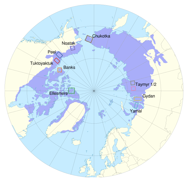
Figure 1 Overview of the study sites. The study sites are distributed around the Arctic with four study sites in northern Canada, one located in Alaska, and five in Siberia. The purple area shows the zone of continuous permafrost (Brown et al., 2002).

The study sites are located in the Arctic tundra and the boreal–tundra transition regions within the continuous permafrost zone (Brown et al., 2002). These regions have different environmental properties including permafrost type, topography lake-abundance, and vegetation type, so we selected representative locations for our study sites. We based the exact outline of the study sites on the Sentinel-2 tiling to facilitate the data processing steps.

The amount of ground ice on a pan-Arctic scale has not been well characterized, but estimations on a coarse scale report ground ice contents of >10 % for all study sites (Brown et al., 2002). On large scales, high ground ice content is associated with the climatic history (e.g. syngenetic ice wedges) and the associated extent of past glacial ice (e.g. buried glacial ice). On small scales ground ice content can vary due to, for example, soil type (Lacelle et al., 2004).

The study sites on Peel, Banks, Ellesmere, Noatak, and Chukotka show strong variation in topography with elevation changes of several hundred metres inside the study sites. The remaining sites show only small variation in elevation (<100 m). Another difference between the study sites is in the number of lakes present. The study sites with the highest number of lakes are in Tuktoyaktuk and Taymyr 2. We found only a small number of lakes on Ellesmere and in Noatak (Table 1).

Table 1 Overview of study sites with size, lake area percentage, elevation range, and number of processed TanDEM-X observations.

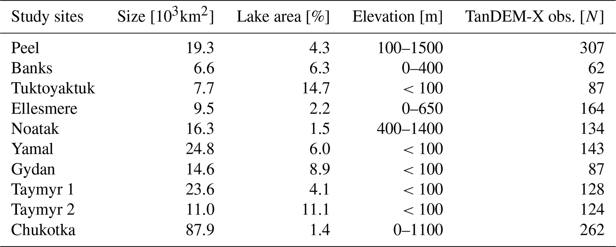
Note that we calculated the lake area percentage using the generated waterbody mask. Here we did not include open waterbodies in the calculation.

3 Methods

3.1 Data and processing

For the DEM generation we used TanDEM-X observations acquired between 2010 and 2017. To ensure adequate vertical accuracies, we only used acquisitions with a height of ambiguity smaller than 80 m (Martone et al., 2012). The radar incidence angles range from 36 to 44^∘. For an accurate orthorectification we used the TanDEM-X 12 m DEM pixel resolution as reference and iteratively updated the look-up table based on the measured deviation (Leinss and Bernhard, 2021). We only studied winter acquisitions because vegetation, wet snow, and standing water during the thaw season induce sizeable errors (Bernhard et al., 2020), whereas in winter we expect the low average monthly temperature to produce a dry snowpack through which radar waves can propagate to the ground without being strongly affected (Millan et al., 2015; Leinss and Bernhard, 2021). We followed a standard approach to generate the DEMs (Fritz et al., 2011), which have a planimetric resolution of about 10 to 12 m and vertical accuracies of about 2 m in areas with high coherences. We did the interferometric processing using the GAMMA Remote Sensing software (Werner et al., 2000). More processing details including tilt removal and the correction of misalignments, specifically for DEMs generated from InSAR observations in permafrost regions, can be found in Bernhard et al. (2020).

3.2 RTS detection and manual mapping of affected areas

In the next step we averaged and mosaicked DEMs corresponding to the same winter. We then used an automated detection algorithm to identify significant elevation changes in the DEM difference images from DEMs that were obtained more than 3 years apart (Bernhard et al., 2020). For each detection we carried out several processing steps. First we assessed the topography and environment using a TanDEM-X DEM and Sentinel-2 multispectral images taken in summer (snow-free). For all study sites at least one Sentinel-2 image during the years 2016 to 2019 was available. The criteria for classifying a detection as an active RTS were the exposure of bare soils, a retreat over time, a location related to a potential sediment removal mechanism, and the presence of a headwall (Lantuit and Pollard, 2008; Nitze et al., 2018; Lewkowicz and Way, 2019). In uncertain cases we used additional time series of Planet RapidEye optical data to classify the detections (Planet-Team, 2018).

The error sources and uncertainties that govern the lower RTS detection limit in terms of the headwall height and retreat rate are manifold and difficult to quantify. This is mainly due to the small number of high-resolution, three-dimensional RTS inventories available (Swanson and Nolan, 2018; Van der Sluijs et al., 2018), where the timescale on which the RTSs are monitored also plays an important role. To obtain an estimate on the lower limit of RTS-induced elevation changes that are detectable, we analysed the smallest RTSs detected in our sample. The 10 smallest RTSs detected have elevation changes in the range of 1.6 to 1.9 m, which is on the same order as the general accuracy of the TanDEM-X DEM and thus represents the smallest RTS headwall heights that are detectable. Similarly, the smallest total area changes of detected RTSs are on the order of 500 to 1000 m², corresponding to about 10 to 12 pixels. Additionally, processes related to the observation properties and InSAR processing further complicate the error estimations. For example, the 40^∘ right-looking viewing geometry leads to different pixel resolutions depending on the aspect and slope of the observed area. These error sources and increased uncertainties should be considered in the interpretation and future use of the dataset, especially for small RTSs, in terms of both horizontal and vertical changes.

After the classification step, we generated polygons for each detected RTS, outlining the area with significant elevation changes. Examples of the generated polygons are shown in Figs. S1 to S4 in the Supplement. The polygons outlining the area of elevation change were drawn by a trained student and the first author, as our use of an automated method that implemented a fixed threshold on the elevation change gave unreliable results. We attributed the RTS polygons in terms of location as either “shoreline” (located close to a waterbody) or “hillslope” (located at trenches or riverbeds).

3.3 RTS attributes

For all calculations we used the polygons, which indicate an area of elevation change and thus a net volume loss. We note that this area can also include a zone of deposition, especially for small and low-relief RTSs or if the time between observations increases. We could not accurately detect areas such as the debris tongues or zones of alluvial deposits, and they are not included. We computed the volumetric and area change as well as the slope and aspect. For parts of the study sites additionally to the winter in 2011/12, observations in 2010/11 and/or 2012/13 were available. To simplify the analysis we normalized the properties to changes per year and took the average if several DEM difference pairs were available. It is important to note that unlike most landslides, RTSs are multi-year features with a strong variability in the erosional intensity as well as a potential change in their morphology over time. In the interpretation of the results and specifically the comparison to landslide studies, the use of the integrated change over several years needs to be considered. We computed the aspect and slope by using the pre-disturbed elevation model and applied Gaussian smoothing with a standard deviation corresponding to 100 m to reduce the influence of random errors (Kang-tsung and Bor-wen, 1991). For the aspect distribution we additionally computed the aspect distribution weighted by volume.

To quantify the volumetric change rate density (volumetric change rate per unit area), we first use a simple approach by dividing the summed total of all RTS volumetric changes per year by the study site size. This has a drawback because RTSs often occur heterogeneously and the result strongly depends on the exact outline of the study sites (Ramage et al., 2017). For example, in the Peel study site only the east-facing part of the mountain range experiences RTS development, but our study site also includes the western part of the range where nearly no RTS activity was detected. To account for this problem, we follow a similar approach to that proposed in Kokelj et al. (2017) and divide our study site into tiles of size 10 km by 10 km, count the number of empty grid cells, and compute a more representative RTS density using only the cells showing RTS activity. It is of note that to interpret the computed density values, the number of empty as well as the number of non-empty grid cells in relation to the total size of the study site should be considered.

To quantify the number of lakes in each study site we used the waterbody mask generated from Sentinel-2 data and computed the area that is covered by the mask (McFeeters, 1996; Kaplan and Avdan, 2017). For this computation, we excluded open-water areas.

We investigated the dependency of RTS growth on different terrain controls by computing the aspect, slope, and location (lakeshore or hillslope). For the aspect we identified the most dominant orientation by summing the number of RTSs as well as the volumetric and area change rates in eight aspect bins (N, NE, E, SE, S, SW, W, NW) and used these bins to compute the strength and orientation of the primary direction.

3.4 Change rate distributions

Figure 2 Schematic representation of RTS area probability density function. Two parts can be distinguished: an exponential-decay part above the cutoff value and a deviation from the power law scaling below the cutoff point.

The probability density function (PDF) of the area affected by elevation loss per year corresponding to an RTS inventory can be defined as

$$\begin{array}{}\text{(1)}& p\left(A_{\mathrm{RTS}}\right)={\displaystyle \frac{\mathrm{1}}{N_{\mathrm{RTS}}}}{\displaystyle \frac{\mathit{\delta }{N}_{\mathrm{RTS}}}{\mathit{\delta }{A}_{\mathrm{RTS}}}},\end{array}$$

where A_RTS is the area change affected by elevation loss of an RTS per year, N_RTS the total number of RTSs in the inventory, δN_RTS the number of RTSs with affected areas between A_RTS and A_RTS+δA_RTS, and δA_RTS the bin width. Equivalently the probability density function p(V_RTS) for the volumetric change per year can be defined.

All RTSs in the study show changes per year in the range of 10² to 10⁶ m² yr⁻¹ for the area and 10² to 10⁶ m³ yr⁻¹ for the volume, and we used 30 bins sampled in log space to cover these ranges.

When analysing a landslides PDF three quantities can be used to describe the distribution: the rollover and cutoff points for small events and the coefficient of the power law scaling β for large events. The rollover point is defined as the peak in the PDF and corresponds to the most common occurrence in the distribution. For large RTSs the PDF can be described as a power law function. The point at which the distribution starts to follow a power law is defined as the cutoff point (Fig. 2).

To determine how well the data points are described by this model and to estimate the rollover point, we fitted a three-parameter inverse gamma function to the RTS probability density function (Malamud et al., 2004). To estimate the error of the fit we used the bootstrap method, drawing 1000 random samples with replacement from all data points and computed the R² value as well as the rollover point for each iteration (Ohtani, 2000).

For the computation of the cutoff value and the exponential scaling exponent, we used the method of Clauset et al. (2009), which is commonly used in landslide frequency–area analyses (Bennett et al., 2012; Parker et al., 2015; Tanyaş et al., 2018). The approach is based on sampling all possible cutoff values and estimating the corresponding exponential scaling coefficients β using a maximum-likelihood fitting method. We then tested the obtained fitting values based on a Kolmogorov–Smirnov statistic and used the values that follow best a true power law distribution as the final cutoff and β value. To quantify the uncertainty we again used a bootstrap algorithm.

3.5 Area–volume scaling

One important quantity in comparing landslides of various sizes is the change relation between area and volume. The simplest conversion assumes that an anisotropic scaling exponent, α, relates the area and volume by V≈A^α. Since both variables (area and volume) are affected by measurement errors, we used an orthogonal distance regression model to fit a straight line (Boggs and Rogers, 1990; Markovsky and Van Huffel, 2007). To quantify the goodness of the fit, we calculated the RMSE, R², and p value (in log space).

4 Results

We investigated 10 different study sites and measured the area and volumetric change rates of 1854 RTSs over a 4- to 5-year timeframe. Due to the low density of RTSs in Yamal and Gydan and the two study sites in Taymyr, we combined these pairs of sites into one study site each (in the following “Yamal/Gydan” and “Taymyr”) according to their geographical and geophysical proximity.

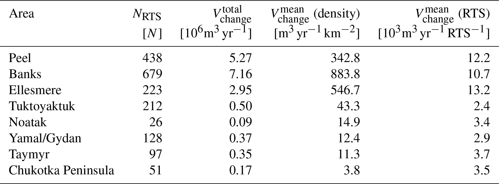
The number of RTSs per study site and the obtained volumetric change rates in terms of the total volume, density, and changes per RTS are shown in Table 2. We found the largest RTSs in terms of average volumetric change rates per RTS at Ellesmere, Peel, and Banks with yearly average change rates of 13 200, 12 200, and 10 700 m³ yr⁻¹. The other areas show much smaller yearly average volumetric change rates in the range of 2400 (Tuktoyaktuk) to 3600 m³ yr⁻¹ (Taymyr). Compared to the other study sites, RTSs at Ellesmere, Peel, and Banks also show higher volumetric change in terms of overall change both per study site size (density) and per individual RTS. Furthermore, these three sites also contain the largest overall size of RTSs of the investigated study sites (Fig. 3).

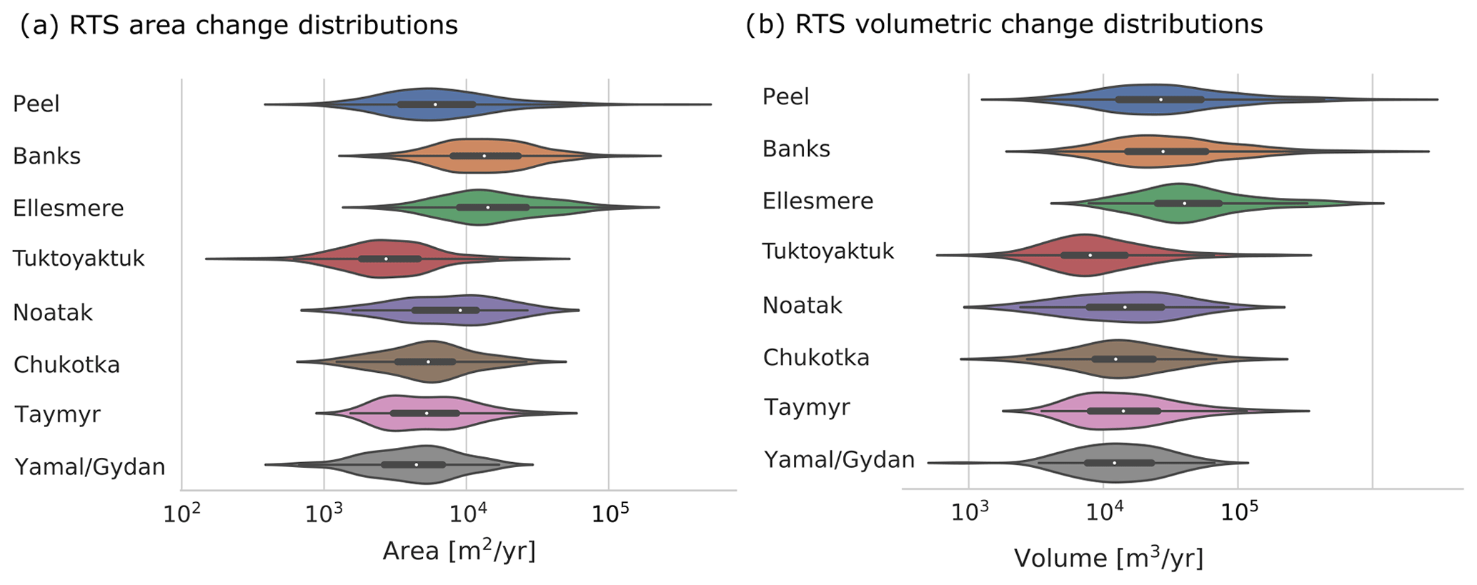
Figure 3 Area (a) and volumetric (b) change rate distributions of mapped RTSs in the form of violin plots. For each violin plot the white dot on the centre line indicates the mean value, the thick centre line shows the interquartile range, the thin centre line shows the total range of data, and the coloured area indicates the probability density of the data across the distribution of values smoothed by a kernel density estimator.

In the following paragraphs we will present (1) a characterization of the area and volumetric changes rates with special emphasis on the probability density functions with the estimation of the rollover, cutoff, and exponential-decay components; (2) the estimated area-to-volume scaling laws; and (3) several terrain controls that could potentially be related to RTS size and frequency. To compare the quantities estimated in the next three sections, we computed the correlation coefficients between them.

Table 2 Number of RTSs in each study site with the total number of RTS and the volumetric change rates in terms of total change, density, and average rates per RTS.

4.1 RTS volume and area distributions

The estimated PDFs are shown in Fig. 4a and b. For most areas the quality of fit of the inverse gamma function was good, as indicated by R² values >0.75. Exceptions were the Noatak and Chukotka study sites with R² values between 0.6 and 0.7. These two sites also have the lowest number of RTSs in the sample with only 26 (Noatak) and 51 (Chukotka) RTSs (Fig. 4c and d).

The modes of the volume change distributions (rollover points) differ between sites. The two study sites located in the high Arctic (Ellesmere and Banks) show rollover values that are an order of magnitude higher. The range of measured volumetric and area change rates show large variations for the Tuktoyaktuk and Peel study sites, whereas the other study sites show smaller variations.

The PDFs above the cutoff value and the relation between rollover and cutoff as well as the exponential-decay values differ between sites (Fig. 5). For the PDF based on the volumetric change, a high rollover value is moderately associated with high cutoff values, indicated by a correlation coefficient of 0.72. By contrast, the PDF based on the area change rate shows a much stronger separation between the high-Arctic sites and the other study sites and consequently also shows a high correlation factor of 0.96. For the power law exponent for RTSs above the cutoff values, no large difference between the areas is visible (β is approximately 2 to 3, and correlation coefficients are <0.64). All correlation coefficients are shown in the Supplement (Fig. S5). It is of note that for the yearly area and volumetric change rates the cutoff value for the Peel study site is relatively small but the distribution continues to high values with yearly area change rates of up to 6×10⁴ m² yr⁻¹ and 3×10⁵ m³ yr⁻¹ (mega-slumps). The computed values of the rollover, cutoff, and exponential-decay coefficients as well as the fit parameters for the inverse gamma function are reported in Tables S1 and S2 in the Supplement.

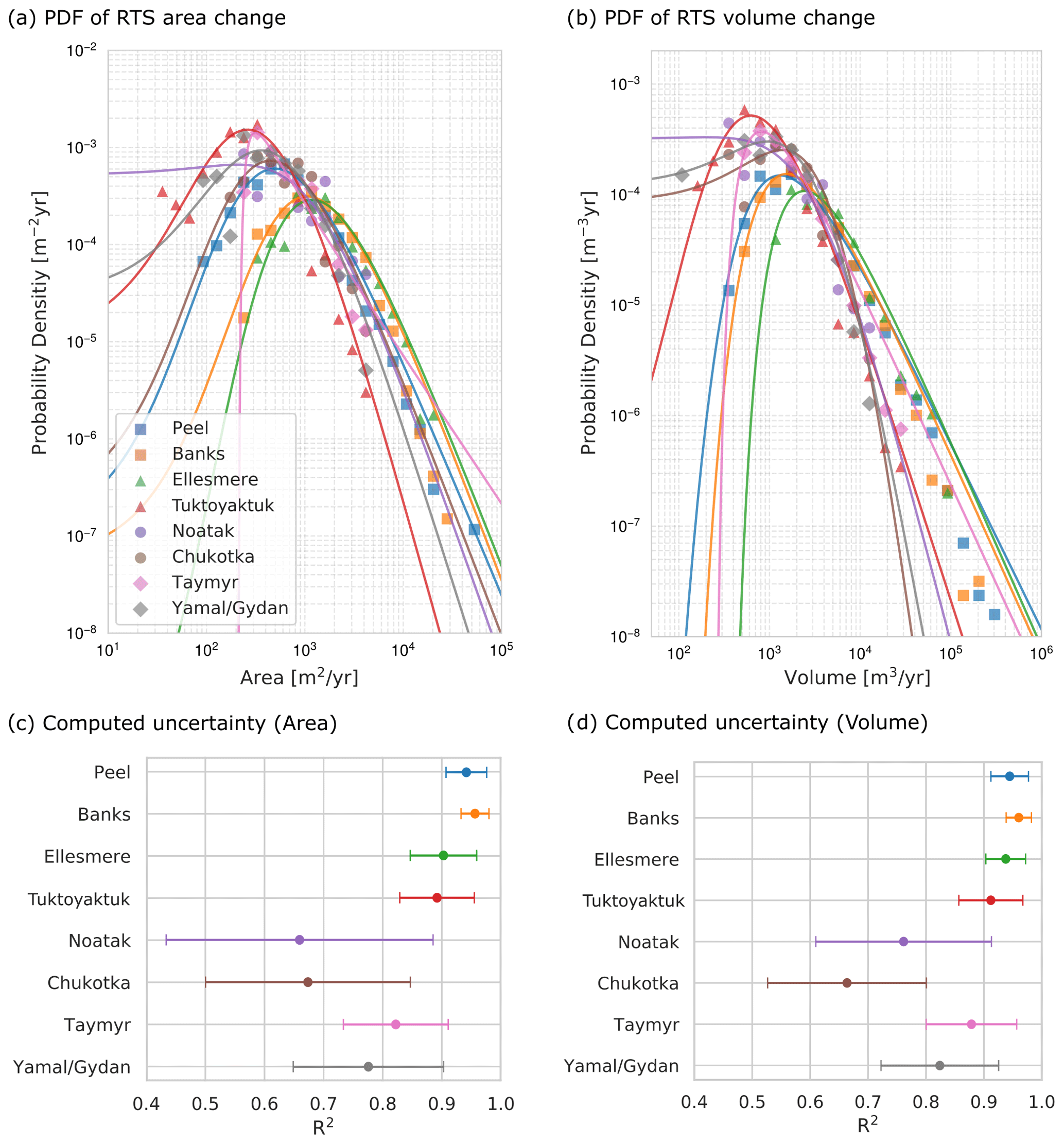
Figure 4 PDF of area and volumetric change rates of mapped RTSs for the set of study sites. Panels (a) and (b) show the PDFs of area and volumetric change rates, respectively, with fitted inverse gamma functions. Panels (c) and (d) show the respective computed R² errors.

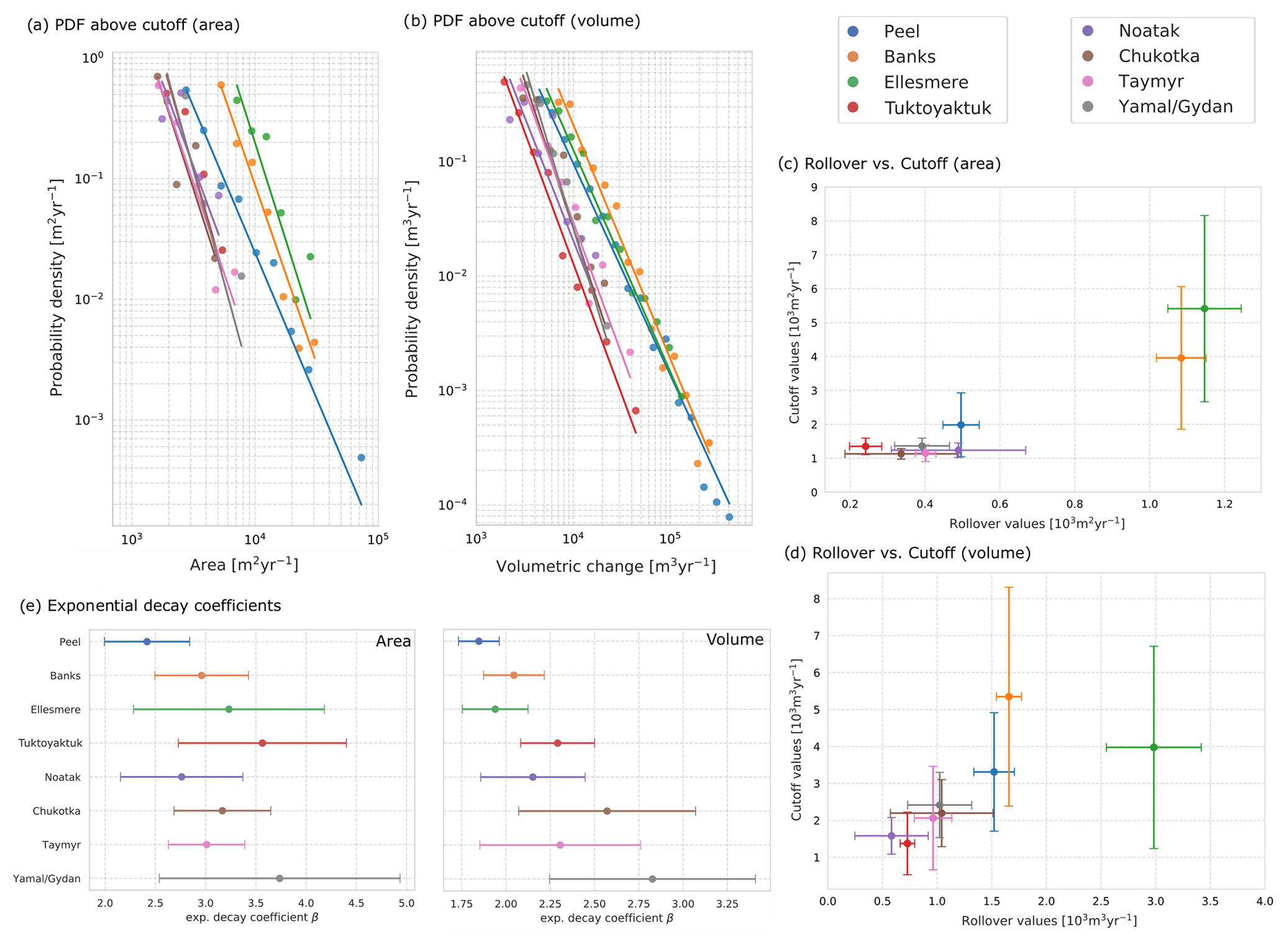
Figure 5 Cutoff, rollover, and exponential-decay coefficients. Panels (a) and (b) show the PDFs for yearly area and volumetric change rates, respectively, above the cutoff values. Panels (c) and (d) shows the respective estimated rollover and cutoff values for yearly area and volumetric change rates. (e) Exponential-decay coefficients for fits above the cutoff.

4.2 Area-to-volume scaling

The estimated area-to-volume scaling law based on all data points in log–log space shows a clear relationship that spans over 4 orders of magnitude between the area and volumetric change rates (Fig. 6a). The estimated scaling exponent across all study sites was $\mathit{\alpha }=\mathrm{1.15}\pm \mathrm{0.01}$. The quality of fit was decent, with an R² value of 0.81, RMSE of 0.21 m³ yr⁻¹, and p value smaller than 10⁻⁶, showing a strong dependency between RTS area and volumetric change rates. This is remarkable considering that RTSs in the sample occurred in different topographic and geomorphological settings. Nevertheless we found a moderate inter-region variability in the scaling coefficient. The α coefficients for the individual sites was in the range of 1.05 to 1.25 with the exception of RTSs in the Banks site with a high coefficient of 1.37 (Fig. 6b). The data points and fitted lines for each study site individually can be seen in the Supplement Fig. S6. The strong association between area and volume change rates can facilitate the estimation of volume changes from multispectral satellite images.

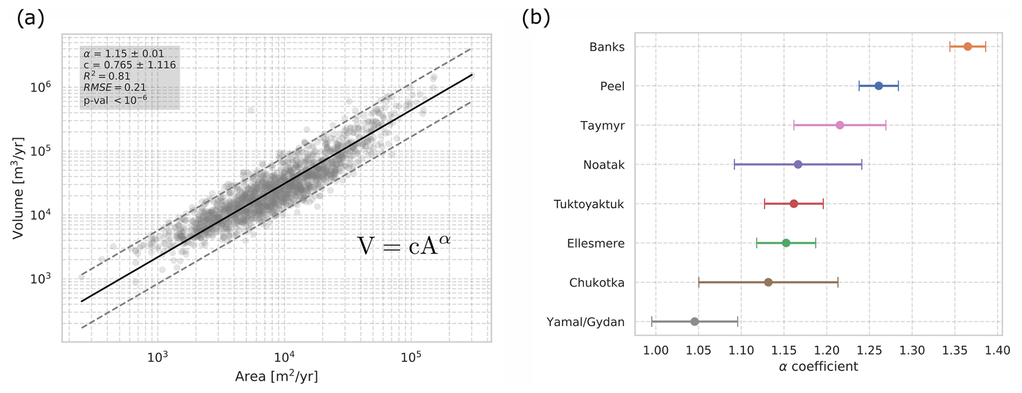
Figure 6 Area-to-volume scaling laws for RTS in the set of study sites. (a) shows the total dataset with all study sites combined. We found an exponential scaling exponent of $\mathit{\alpha }=\mathrm{1.15}\pm \mathrm{0.01}$. (b) shows the computed values of the scaling exponent, α, for each site individually with the estimated standard deviation. A large variation between 1.05 and 1.37 is visible.

4.3 Terrain controls

Among the investigated terrain controls, aspect shows the greatest variability between the study sites. RTSs located in Siberia as well as on Ellesmere tend to favour a south-west-facing orientation (Fig. 7a). The very small number of RTSs in the Noatak study site showed a preferred orientation towards the north-west, and RTSs in Peel have a preferred orientation towards the north-east. For Tuktoyaktuk and Banks no clear trend is visible. To consider the possibility of more than one preferred orientation, we additionally looked at the initial aspect bin distribution (Supplement Fig. S7). Here only the aspect distribution of RTSs in the Noatak Valley shows two preferred orientations, but this could be related to the low number of RTSs in the study site. Additionally to the number of RTSs in each aspect bin, we weighted the aspect by the volumetric change rates. This only slightly alters the preferred orientation, and large RTSs do not occur at different aspects.

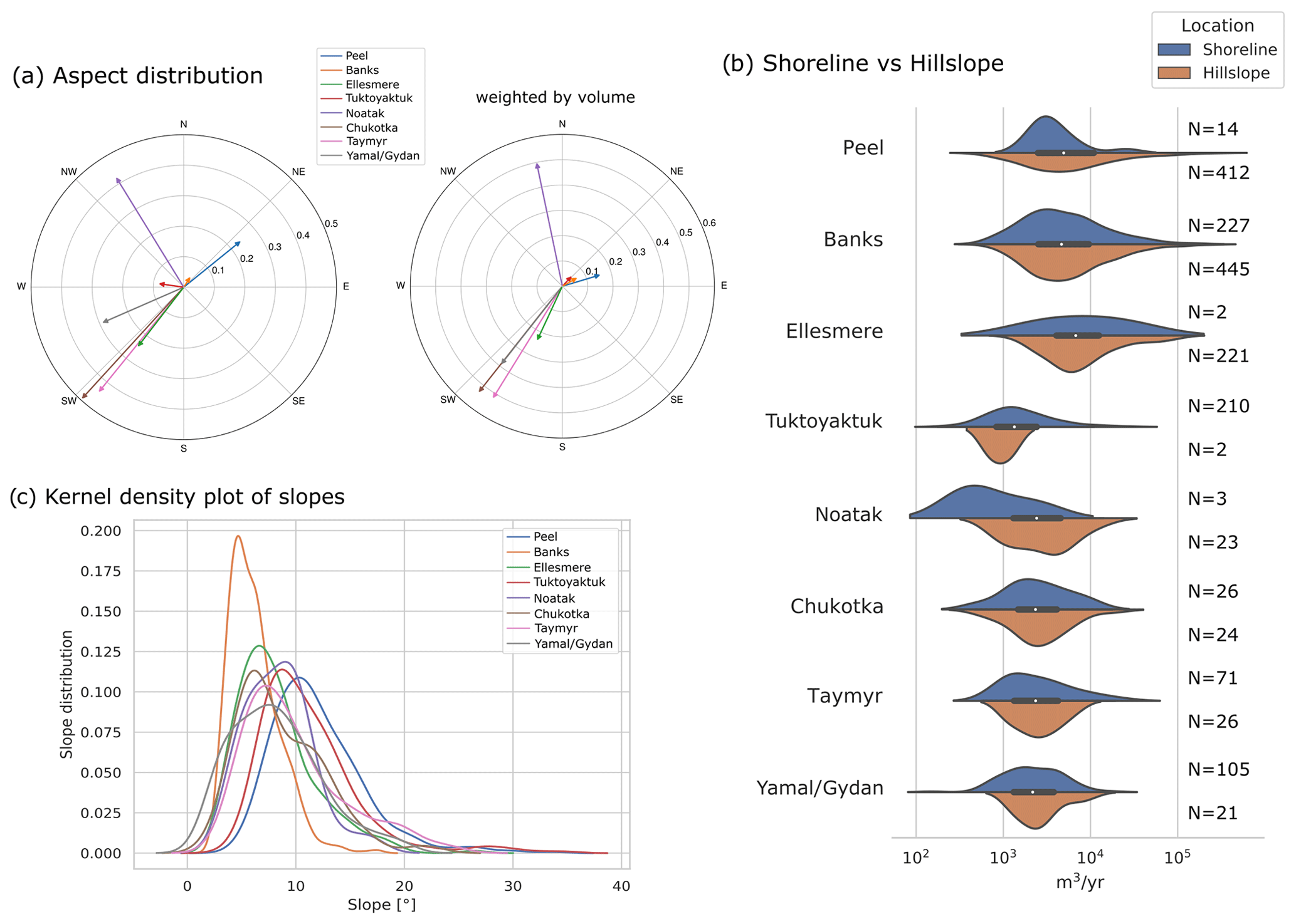
Figure 7 Terrain controls of mapped RTSs for each study site. Panel (a) shows the aspect main orientation of RTSs in each study site (left) and this additionally weighted by the volumetric change rates (right). Panel (b) shows the probability density distributions of volumetric changes rates in the form of violin plots. For each violin plot the white dot on the centre line indicates the mean value of the entire study site dataset, with the thick centre line showing the interquartile range. However, the top part of each violin indicates the probability density of the subset of shoreline RTSs, whereas the bottom part indicates the probability densities of the subset of hillslope RTSs, and the data across the distributions of values are smoothed by a kernel density estimator. The number of RTSs in each subset is listed on the right. Some sites are dominated by one location type. Panel (c) shows the distribution of the pre-disturbed DEM slopes at the RTS locations.

The slope of the pre-disturbed area shows some difference between the study sites (Fig. 7c). In general all RTSs evolve at slopes ranging from 2 to 3^∘ up to slopes of 20^∘. Interestingly, in the study site of the largest RTSs on Banks, they tend to favour lower slopes with values below 12^∘.

We investigated the dependency of RTS locations in terms of their occurrence. We distinguished two types of location, either at a shore (including lake and coastal) or at hillslopes with no large waterbodies close by. Several study sites have mostly one type of RTS location. The RTSs in Ellesmere (99 % hillslope), Peel (96 % hillslope), and Noatak (88 % hillslope) have mostly RTSs at hillslope locations. On the contrary, RTSs in the Tuktoyaktuk site are nearly all located at lakeshores (99 %). All other study sites have a mixture of hillslope and shoreline RTS locations: Banks (66 % hillslope), Chukotka (52 % hillslope), Taymyr (27 % hillslope), and Yamal/Gydan (26 % hillslope). In the study sites with both types of RTS location, no significant difference between the distributions is visible (Fig. 7c). Furthermore, we did not find a significant correlation between RTS size and the percentage of hillslope or shoreline RTS locations (Supplement Fig. S5).

To estimate the volumetric change rate density of RTSs within the RTS-affected regions of each study site, we gridded them into tiles of size 10 km by 10 km. Figure 8a shows the volumetric change rates per square kilometre using only the tiles with RTSs present. The volumetric change densities over the total study site strongly depend on the exact outline of study sites, and removing tiles without RTSs present gives a more consistent and comparable volumetric change rate density. To make this more visible, the number of tiles with RTSs present and without can be seen in Fig. 8b. Here for example, the Chukotka Peninsula has only a small number of tiles with RTSs present.

Figure 8 Volumetric change rate densities (a) and density related to study site size (b) for each study site. Panel (a) shows the computed RTS volumetric change rate densities using a 10 km by 10 km grid with the empty grid cells removed. The vertical bars indicate the range in the computed densities. Panel (b) shows the study site size with the fraction of tiles with RTSs represented by the solid colour.

5 Discussion

5.1 Probability density functions to characterize thaw slump activity

The computed probability density functions of the yearly area and volumetric change rates follow a characteristic inverse gamma law with first an increase in frequency up to a maximum value with the most abundant thaw slump sizes (rollover) and then a decrease with an exponential-decay tail above a certain cutoff value. Our findings show that the applicability of this universal scaling also applies to permafrost landscapes, despite differences in the governing geomorphic processes with respect to lower-latitude environments. Here we emphasize again that another difference between our analyses and those of common landslide studies is that RTSs are a multi-year phenomena with variable yearly erosion rates. Some variability in the exact form of the distributions should therefore be expected if different time periods are chosen.

To further investigate the distributions we distinguish between two parts: (1) the exponential-decay part for large RTSs and (2) the part that deviates from this exponential decay below the cutoff point. For landslides the exponential-decay part is typically explained in a statistical way by the concept of self-organized criticality, where a constant “input” of a specific landslide size at a random location, together with a merger of landslides that are close to each other, reproduces this distribution (Bak and Tang, 1989; Turcotte, 1999). For RTSs this explanation seems plausible since initiation and evolution are strongly linked to soil properties that can promote RTS development in close proximity and also since RTS coalescence is common (Lantz and Kokelj, 2008; Lantuit et al., 2012; Wang et al., 2016). In addition to the universal exponential-decay behaviour in all study sites, we found that the largest RTSs in the Peel, Banks, and Ellesmere study sites have growth rates that are orders of magnitude larger (Fig. 5a and b). A possible explanation is that topographic and geomorphological properties, like the amount of massive ice, overburden thickness, or the steepness of terrain, only allow RTSs to grow to a certain size (Kokelj et al., 2017; Rudy et al., 2017; Jones et al., 2019). For example in the Tuktoyaktuk study site (N_RTS=212) where RTSs occur at lakeshores in mainly flat regions, the largest RTSs show growth rates of between 5200 m² yr⁻¹ and 31 800 m³ yr⁻¹ compared to, for example, the Ellesmere site (N_RTS=223) with more topographic features and mainly hillslope RTSs, which show maximum growth rates that are 3 to 4 times higher (range is between 23 000 and 106 400 m² yr⁻¹). This suggests that additionally to the exponential-decay factor, a maximum RTS growth rate is also important to characterize the high end tail of the probability density function.

For the deviation from the exponential decay, two types of explanation have been proposed for landslides in temperate climate (Tebbens, 2020): first an under-sampling of small landslides due to limitations in resolution and secondly an explanation that attributes this divergence to physical processes. Investigating our dataset, a divergence due to under-sampling seems unlikely since the PDFs in Peel, Banks, and Ellesmere show this divergence (cutoff point) at high yearly change rates of >10⁴ m² yr⁻¹ and $>\mathrm{3}\times {\mathrm{10}}^{\mathrm{4}}$ m³ yr⁻¹, which corresponds to area and volumetric changes high above the resolution limit (TanDEM-X DEM resolution – horizontal ≈10 m, vertical 2 to 5 m). The physical origins are likely related to environmental conditions and physical characteristics of ground materials like ground ice content but are outside the scope of this work. Future models for thaw slump initiation and evolution should be able to investigate the drivers and reproduce such distributions.

5.2 Similarities and differences in area–volume scaling

We found a power law relationship (V≈A^α) between the area and the volumetric change rates with a scaling coefficients α of 1.15 for the total dataset and ranging between 1.05 and 1.37 for the individual study sites. Such relationships are known from landslides in temperate climates with typically values of 1 to 1.5 (Larsen et al., 2010; Klar et al., 2011). For RTSs only one study by Kokelj et al. (2021), investigating RTSs on the Peel Plateau and Richardson Mountains, has estimated this relationship, and it found a scaling coefficient of 1.42, which is relatively high compared to our values (Peel – 1.27, Tuktoyaktuk – 1.17) but inside the estimated error.

Comparing the coefficients between study sites, we found that lower scaling coefficients are not correlated with smaller RTSs. For example the scaling law coefficient in the Tuktoyaktuk site with relatively small RTSs is the same as for the RTSs in the Ellesmere site with the largest RTSs in our dataset. On the other hand, for RTSs in the Peel study site there is little confining topography and deep layers of ice-rich tills that allow the headwalls to grow to large sizes and consequently yield a steeper regression curve (Lacelle et al., 2015). The diversity in landform characteristics also contributes to the variation in the area-to-volume scaling coefficient. At the study sites Banks and Noatak, shallow detachments are dominant in the small-area range. These may promote larger scaling coefficients when combined with older, deeper RTSs (Lewkowicz, 1987b). Furthermore, most RTSs initiate as shallow active layer detachments. The gradual increase in headwall heights following the initiation event could lead to a temporal change in the scaling coefficient. Further investigations relating the scaling coefficients to additional RTS and area characteristics (e.g. soil properties, climatic history, age of the RTSs) are needed.

5.3 Terrain controls and their relation to RTS size

With the available data we could determine several terrain controls, namely the orientation of RTS growth and the slope of the pre-disturbed area the RTS grew into as well as the location in terms of hillslope and shoreline RTSs. Our findings in terms of the preferred orientation of RTSs are mostly consistent with past regional studies: a preferred south-west orientation for RTSs in the Siberian study sites (Nesterova et al., 2020) and Ellesmere (Jones et al., 2019), towards the north-east for the Peel study site (Lacelle et al., 2015), and north-facing RTSs in Noatak (Swanson and Nolan, 2018). For RTSs in the Tuktoyaktuk study site we found no preferred orientation, which is consistent with Wang et al. (2009) but in contradiction to other studies that found RTSs orientations that favour north-facing slopes (Kokelj et al., 2009; Zwieback et al., 2018, 2020). The association with aspect hints at inter-regional differences in the governing geomorphic drivers and controls. A south-west-facing orientation is considered to be related to higher initiation and growth rates of RTSs due to the higher energy available from solar radiation (Lewkowicz, 1987a). This would suggest that solar radiation is an important factor in RTS growth and initiation for the study sites in Ellesmere and Siberia. Past studies have shown that a high ground ice content is a necessary condition for RTS development (Kokelj and Jorgenson, 2013; Ramage et al., 2017). During the Holocene thermal maximum, the regions in north-west Canada experienced warmer summer temperatures than other Arctic regions and could have lost ground ice on south-facing slopes (Burn et al., 1986; Kaufman et al., 2004; Lacelle et al., 2010; Zwieback et al., 2018). Thus the differences in RTS aspect distributions could be related to the climatic history. For example the dominant north-facing exposure on the Peel Plateau could reflect such anisotropic abundance of ground ice.

We did not find a significant relation between RTS size (area and volumetric change rates) and aspect as well as slope or location (hillslope, shoreline). This finding affirms previous studies that have highlighted the complexity of the processes and controls governing RTS expansion.

5.4 Implications

The scaling relations we quantified are critical for modelling and predicting RTS activity and the impacts on biogeochemical cycling. The regional variability in scaling behaviour needs to be considered when upscaling field observations to estimate large-scale nutrient, sediment, and carbon budgets. Because Earth system models strive to capture the variability in these processes from regional to global scales, our results can be used to calibrate and validate global models. Possible changes in the scaling relations could be important indicators to predict future RTS evolution and impacts.

Our observations of variable RTS development rates and regimes highlight the need for continual pan-Arctic monitoring and further satellite missions to derive high-resolution DEMs. The TanDEM-X data availability only allowed us to compute elevation changes in a 5-year time window. To investigate changes in RTS activity related to climate change, a higher temporal resolution is needed. Here additional observations from the TanDEM-X satellite as well as data from the ArcticDEM could add additional data points (Bachmann et al., 2018; Dai et al., 2020). Furthermore, with the derived area-to-volume scaling laws it is potentially possible to use optical satellite images which are available at a higher temporal resolution to estimate the volumetric change.

6 Conclusions

In this study we quantified the yearly volumetric and area change rates of RTSs over a 5-year timeframe in 10 study sites across the Arctic with a total study size of 220 000 km² and a total number of 1868 RTSs. We found that the frequency distributions of the volumetric and area change rates are well described by an inverse gamma distribution (R²>0.5) with the distinct features of a rollover, cutoff, and exponential decay for large RTSs. This kind of behaviour is well known for landslides in temperate climate regions with very different trigger mechanisms and soil properties and could provide valuable insights into modelling future RTS evolution on a pan-Arctic scale.

The comparison between study sites showed that the distribution of RTSs in northern Canada (Peel Plateau and Richardson Mountains, Banks Island, Ellesmere Island) is shifted towards higher change rates in volume and area than elsewhere in the Arctic. Nevertheless, the exponential-decay rates for large RTSs in all study sites were similar.

Our analyses revealed consistent but regionally variable area-to-volume scaling behaviour. For the total dataset we found a scaling coefficient of $\mathit{\alpha }=\mathrm{1.15}\pm \mathrm{0.01}$ with some variance between the study sites (α between 1.05 to 1.37).

We examined terrain controls on RTS distributions, including slope, and adjacency to waterbodies, but aspect showed the greatest association with RTS occurrence, though it varies regionally. We found diverse preferred orientations of RTSs between the study sites from no dominant orientation for Tuktoyaktuk and Banks Island, a north-east orientation for the Peel Plateau and Richardson Mountains, east-facing RTSs in the Noatak Valley, and a strong south-west orientation of all study sites in Siberia and the study site on Ellesmere Island.

Our regionally variable RTS scaling relations may be used to constrain large-scale estimates of carbon, sediment, and nutrient budgets. By capturing the variability in RTS change rates across scales, remote sensing is a vital tool for predicting hazards and attendant ecosystem changes in a rapidly changing Arctic.